Delay-Dependent Stability of Impulsive Stochastic Systems with Multiple Delays

Abstract

This paper associates with stability analysis of linear impulsive stochastic delay systems (ISDSs). Although many conclusions about the stability of ISDSs have been obtained based on Lyapunov’s method, relatively few research theories about delay-dependent stability with less conservativeness have been established. Therefore, we introduce an appropriate Lyapunov-Krasovskii functional (LKF) to work out this problem, and a novel delay-dependent exponential stability theorem is first deduced. On the other hand, when mean-square stability is considered, we present delay-dependent stability conditions, it is of interest to note that the proposed conditions do not depend on the size of delays in the diffusion term, which solves the problems of determining the mean-square stability of ISDSs for which the diffusion term delays are not available. In the end, two numerical examples are carried out to verify the feasibility of our conclusions.

1. Introduction

The presence of time-delays frequently affects real life such as biology, engineering, communication, and the long-distance-transmission systems, etc (see, e.g., [1,2,3]). Such delays may have significant influences on the overall behavior of a dynamical system and result in oscillation, poor performance, and even instability. Therefore, the investigations about the stability of time-delay systems (TDSs) have become topical issues in the past few decades (see, e.g., [4,5,6,7,8,9]). In accordance with the dependence of stability conditions on delays, the criteria for stability of TDSs come in two varieties: those named delay-independent stability (DIS) criteria and those that are delay-dependent stability (DDS) criteria (see, e.g., [10,11,12,13]). Generally, the DDS conditions may be less conservative than DIS conditions, especially for the small delays. For instance, Ref. [10] obtained the DDS criterion of uncertain TDSs, which can be verified by solving related LMIs. Furthermore, impulsive systems have been carefully conducted in [14,15] since they construct a mathematical framework for the dynamic processes whose states experience instantaneous jumps at certain times. Moreover, the extended discussions around stability studies of impulsive delayed systems (IDSs) were presented in [16,17,18]. For instance, in [17], by introducing a switching parameter, input-to-state stability for IDSs was guaranteed by a Razumikhin-type criterion.

At the same time, some structures and parameters of impulsive delay systems are inevitably affected by stochastic perturbation in some real-world progress. In consequence, as a suitable mathematical model to describe impulsive control problems under stochastic noise, impulsive stochastic delay systems (ISDSs) have triggered concerns [19,20,21,22,23]. Therefore, many effective research methods were presented for analyzing the stability of ISDSs, such as the comparison principle, the Lyapunov function, the Lyapunov-Razumikhin theorem, and the LKF method. More specifically, Ref. [24] proposed DDS and DIS criteria for the exponential mean-square stability of stochastic time-delay systems by using the comparison principle. On the basis of the discussions on Lyapunov functions, Ref. [21] obtained some criteria of the global exponential stability for ISDSs. In [22], by employing Razumikhin technique, a few theorems were set up to ensure p-th moment exponential stability for ISDSs with Markovian switching. Specifically, Ref. [23] obtained the p-th moment exponential stability of ISDSs driven by G-motion.

Taking the effect of the actual impulse perturbation into account, we cope with DDS conditions for a kind of ISDSs in this paper. It is well-known that the stability criteria using the Lyapunov function method and the Razumikhin technique require the construction of Lyapunov functions, however, the Lyapunov functions are not easy to construct, so the relevant conclusions are not convenient in practical applications. In contrast, stability criteria given in the form of LMI using the LKF method do not have the trouble of constructing Lyapunov functions, and they can be verified directly by Matlab. Therefore, we obtained sufficient conditions for the mean-square exponential stability of ISDSs by using a suitable LKF, and the DDS conditions obtained may possess less conservativeness. In particular, it is difficult to obtain the diffusion term delays in some real systems. Therefore, for the situation where the diffusion term delays are not directly available, we establish draft-delay-dependent/diffusion-delay-independent conditions for the mean-square stability of ISDSs. In general, the main contributions of our work are as follows:

(i)

A DDS theorem for exponential stability of ISDSs is founded by using an appropriate LKF, which can be verified by the feasibility of LMIs.

(ii)

When mean-square stability is considered, we propose sufficient conditions for this kind of ISDSs, and the established DDS criterion does not rely on the existence of delays in the diffusion term.

Subsequent works can be described in the following sections. Section 2 provides some theoretical necessary stuff. Stability conditions for the linear ISDSs are deeply discussed in Section 3. Two numerical examples and their simulations validate the effectiveness of conclusions in Section 4. Finally, we summarize this paper in Section 5.

In this paper, we use $(\Omega ,\mathcal{F},\mathcal{P})$ on behalf of a complete probability space with a filtration ${\left\{{\mathcal{F}}_t\right\}}_{t\ge 0}$, and the filtration satisfies the usual conditions. $\mathbb{N}=\{0,1,2,\cdots \}$, ${\mathbb{N}}^{+}=\{1,2,\cdots \}$. Let integers e and h satisfy $e<h$, and $\overline{e,h}=\{e,e+1,\cdots ,h\}$. Matrix $B<0(B>0)$ denotes B is a negative definite (positive definite) matrix with $B^T=B$. $|·|$ stands for the Euclidean norm operator, and the mathematical expectation operator is denoted by $\mathbb{E}(·)$. Square matrix $B\in {\mathbb{S}}_{+}^{n\times n}$ means B is a symmetric positive definite matrix. ${\lambda }_{max}\left(A\right)$ (${\lambda }_{min}\left(A\right)$) is the maximum (minimum) eigenvalue of matrix A. For $\tau >0$, $\mathcal{C}([-\tau ,0];{\mathbb{R}}^n)=\{\psi :[-\tau ,0]\to {\mathbb{R}}^n|\psi \left(s\right)$ is a piecewise right continuous function with the norm ${\displaystyle \parallel \psi \parallel =\underset{-\tau \le s\le 0}{sup}\left|\psi \left(s\right)\right|\}}$; ${\mathcal{L}}_{{\mathcal{F}}_0}^2([-\tau ,0];{\mathbb{R}}^n)$ denotes the set of ${\mathcal{F}}_0$-measurable stochastic variables $\psi \in \mathcal{C}([-\tau ,0];{\mathbb{R}}^n)$ satisfying ${\displaystyle \underset{-\tau \le s\le 0}{sup}\mathbb{E}{\left|\psi \left(s\right)\right|}^2<\infty }$. Set ${\displaystyle {\mathcal{L}}_{{\mathcal{F}}_0}^2\left(\delta \right)=\left\{\psi \right|\psi \in {\mathcal{L}}_{{\mathcal{F}}_0}^2([-\tau ,0];{\mathbb{R}}^n),\underset{-\tau \le s\le 0}{sup}{\mathbb{E}\left|\psi \left(s\right)\right|}^2<\delta \}}$. For $B=B^T$, $C=C^T$, we use $\left(\begin{array}{cc}B& D\\ \ast & C\end{array}\right)$ = $\left(\begin{array}{cc}B& D\\ D^T& C\end{array}\right)$ for simplicity.

2. Preliminaries

Consider the following ISDSs with multiple delays:

$$\left\{\begin{array}{c}{\displaystyle dx\left(t\right)=\sum _{i=1}^m{A}_{i}x(t-{\tau }_i)dt+\sum _{i=1}^m{B}_{i}x(t-{\delta }_i)d{w}_i\left(t\right),t\ne t_k,}\hfill \\ \Delta x\left(t_k\right)=C_{k}x\left(t_k^{-}\right),k\in {\mathbb{N}}^{+},\hfill \\ x(t_0+s)=\psi \left(s\right),t_0=0,s\in [-\tau ,0],\hfill \end{array}\right.$$

(1)

for each $i\in \overline{1,m}$, $A_i,B_i\in {\mathbb{R}}^{n\times n}$, $w_i\left(t\right)$ is a scalar Brownian motion defined on $(\mathrm{\Omega },\mathcal{F},\mathcal{P})$. ${\tau }_i\ge 0$ and ${\delta }_i\ge 0$ are the drift term delays and the diffusion term delays, respectively. $\tau ={max}_{i\in \overline{1,m}}\{{\tau }_i,{\delta }_i\}$. $\psi \left(s\right)\in {\mathcal{L}}_{{\mathcal{F}}_0}^2([-\tau ,0];{\mathbb{R}}^n)$ is the given initial value. $\{t_k,k\in {\mathbb{N}}^{+}\}$ is a monotone increasing impulsive switching time sequence, and ${lim}_{k\to +\infty }{t}_k=+\infty$. Let $x\left(t_k^{+}\right)={lim}_{s\to 0^{+}}x(s+t_k)$, $x\left(t_k^{-}\right)={lim}_{s\to 0^{-}}x(s+t_k)$, and $\Delta x\left(t_k\right)=x\left(t_k^{+}\right)-x\left(t_k^{-}\right)$. $\Delta x\left(t_k\right)=C_{k}x\left(t_k^{-}\right)$ is the state jumping at the moment of $t_k$, where $C_k\in {\mathbb{R}}^{n\times n}$ is the impulse gain matrix, $k\in {\mathbb{N}}^{+}$. In addition, for any $\psi \left(s\right)\in {\mathcal{L}}_{{\mathcal{F}}_0}^2([-\tau ,0];{\mathbb{R}}^n)$, we assume there exists a stochastic process, as the solution of (1), is right-continuous, i.e., $x\left(t_k\right)=x\left(t_k^{+}\right)$.

Definition 1.

For any $t_0>0$, a stochastic process $x\left(t\right)\in {\mathbb{R}}^n$ is called to be a solution of (1) on $\left[t_0,T\right]$ ($t_0<T<\infty$) if it satisfies conditions below:

(i) 

The set of impulses $\mho =\left\{t\in \left(t_0,T\right]\mid t=t_k,\right.$ $\left.k\in {\mathbb{N}}^{+}\right\}$ is finite;

(ii) 

For $t\in \mho$, $x\left(t\right)$ is right-continuous, i.e., $x\left(t_k\right)=x\left(t_k^{+}\right)$. $x\left(t\right)$ is continuous for all non-impulsive times (i.e., $t\in (t_0,T]\setminus \mho$) and ${\mathcal{F}}_t-$adapted;

(iii) 

For any $t\in \left(t_0,T\right],\psi \in {\mathcal{L}}_{{\mathcal{F}}_0}^2\left([-\tau ,0]\right.$, $\left.{\mathbb{R}}^n\right)$, the following equation:

$$x\left(t\right)=\left\{\begin{array}{c}\psi \left(t\right),t\in [-\tau ,0],\hfill \\ {\displaystyle x\left(t_0\right)+\sum _{i=1}^m{\int }_{t_0}^t{A}_{i}x(t-{\tau }_i)dt+\sum _{i=1}^m{\int }_{t_0}^t{B}_{i}x(t-{\delta }_i)d{w}_i\left(t\right),t\in (t_0,T]\setminus \mho ,}\hfill \\ C_{k}x\left(t_k^{-}\right),t=t_k\in \mho ,\hfill \end{array}\right.$$

(2)

holds with probability 1.

Next, we recall the definitions of mean-square stability and mean-square exponential stability.

Definition 2

([25]). The trivial solution of (1) is called mean-square stable if for any $\epsilon >0$, there exists $\delta >0$, such that ${\mathbb{E}\left|x\left(t\right)\right|}^2\le \epsilon$$(t\ge 0)$ for any initial value $\psi \in {\mathcal{L}}_{{\mathcal{F}}_0}^2\left(\delta \right)$.

Definition 3

([26]). The trivial solution of (1) is called mean-square exponentially stable if there exist constant $\mathrm{\Gamma }\in {\mathbb{R}}^{+}$, and constant $\gamma \in {\mathbb{R}}^{+}$, independent of the initial value ψ and time t, such that

$${\mathbb{E}\left|x(t;\psi )\right|}^2\le \mathrm{\Gamma }\mathbb{E}{\parallel \psi \parallel }^2{e}^{-\gamma t},t\ge 0,$$

(3)

for any $\psi \in {\mathcal{L}}_{{\mathcal{F}}_0}^2([-\tau ,0];{\mathbb{R}}^n)$.

Definition 4

([26]). For simplicity, let $x_t=x(t+s)$, $s\in [-\tau ,0]$, $V(t,x_t):[0,\infty )\times {\mathbb{R}}^n\to {\mathbb{R}}^{+}$ is said to belong to the class S if $V(t,x_t)$ satisfies the conditions below:

(i) 

For every moment $t_k\in \{t_k,k\in {\mathbb{N}}^{+}\}$, ${lim}_{t\to t_k^{-}}V(t,x_t)=V(t_k^{-},x_{t_k^{-}})$ and ${lim}_{t\to t_k^{+}}V(t,x_t)=V(t_k^{+},x_{t_k^{+}})$ exist in ${\mathbb{R}}^{+}$. Moreover, $V(t_k^{+},x_{t_k^{+}})=V(t_k,x_{t_k})$;

(ii) 

For $t\in [t_{k-1},t_k)\times {\mathbb{R}}^n$, $V(t,x_t)$ is continuously twice differentiable in $x_t$ and once in t.

In order to draw our conclusion more accurately, the following lemma is needed in the subsequent discussions.

Lemma 1

([27]). For matrices $\mathcal{P}={\mathcal{P}}^T$, $\mathcal{M}$, and $\mathcal{Q}$ with appropriate dimensions, the following LMI:

$$\left[\begin{array}{cc}\mathcal{P}& \mathcal{M}\\ {\mathcal{M}}^T& -\mathcal{Q}\end{array}\right]<0$$

is equivalent to $\mathcal{Q}>0$, $\mathcal{P}+\mathcal{M}{\mathcal{Q}}^{-1}{\mathcal{M}}^T<0$.

3. Main Results

In this section, with the help of an appropriate LKF, we will focus our attention on the stability study of (1) and accordingly give sufficient conditions for exponential stability of system (1).

Theorem 1.

Suppose that there exist matrices $M_1\in {\mathbb{R}}^{n\times n}$, $M_2\in {\mathbb{R}}^{n\times n}$, $Q\in {\mathbb{S}}^{n\times n}$, $P\in {\mathbb{S}}_{+}^{n\times n}$, $G_i\in {\mathbb{S}}_{+}^{n\times n}$, $W_{ij}\in {\mathbb{S}}_{+}^{n\times n}$, $i\in \overline{1,m}$, $j\in \overline{1,m}$, scalar α and positive constants ${\xi }_1$, ${\xi }_2$, σ, γ, β satisfying $\beta <1$ and

$$ln(\beta +\frac{2\tau {\xi }_2}{{\xi }_1})<-(\alpha +\gamma )\sigma ,$$

(4)

as well as the following LMIs hold:

$$\begin{array}{cc}& \left[\begin{array}{cccc}-Q+{\mathrm{\Psi }}_1& {\mathrm{\Psi }}_2& M_1^T{\mathcal{A}}^{\tau }& M_1^T\mathcal{A}⨂\mathcal{I}\\ \ast & {\mathrm{\Psi }}_3& M_2^T{\mathcal{A}}^{\tau }& M_2^T\mathcal{A}⨂\mathcal{I}\\ \ast & \ast & -{\mathrm{\Psi }}_4& 0\\ \ast & \ast & \ast & -{\mathrm{\Psi }}_5\end{array}\right]<0,\hfill \end{array}$$

(5)

$${\xi }_{1}I<P,\hfill$$

(6)

$$& {(I+C_k)}^{T}P(I+C_k)<\beta P,k\in {\mathbb{N}}^{+},\hfill$$

(7)

where

$$\begin{array}{cc}\hfill & {\displaystyle {\mathrm{\Psi }}_1=\sum _{i=1}^m[M_1^T{A}_i+A_i^T{M}_1+B_i^{T}P{B}_i+{\tau }_i\sum _{j=1}^m{B}_j^T{W}_{ij}{B}_j],}\hfill \\ \hfill & {\mathrm{\Psi }}_2=P-M_1^T+\sum _{i=1}^m{A}_i^T{M}_2,{\mathrm{\Psi }}_3=-M_2-M_2^T+\sum _{i=1}^m{\tau }_i{G}_i,\hfill \\ \hfill & {\mathrm{\Psi }}_4=diag(G_1,\cdots ,G_m),{\mathrm{\Psi }}_5=diag({\mathcal{W}}_1,\cdots ,{\mathcal{W}}_m),\hfill \\ \hfill & {\mathcal{W}}_i=diag(W_{i1},\cdots ,W_{im}),{\mathcal{A}}^{\tau }=[\sqrt{{\tau }_1}{A}_1,\cdots ,\sqrt{{\tau }_m}{A}_m],\hfill \\ \hfill & \mathcal{A}⨂\mathcal{I}=[{\mathcal{A}}_1,{\mathcal{A}}_2,\cdots ,{\mathcal{A}}_m],{\mathcal{A}}_i=\underset{m}{\underbrace{[A_i,\cdots ,A_i]}},i=1,2,\cdots ,m.\hfill \end{array}$$

If $t_1\ge 2\tau$ and ${\displaystyle {sup}_{k\in {\mathbb{N}}^{+}}\{t_{k+1}-t_k\}\le \sigma }$, then system (1) is mean-square exponentially stable.

Proof. 

Let $g_i\left(t\right)=B_{i}x(t-{\delta }_i)$, and ${\displaystyle y\left(t\right)=\sum _{i=1}^m{A}_{i}x(t-{\tau }_i)}$. First, we introduce a LKF $V(t,x_t)$ ([12]) (see Definition 4) as follows:

$$V(t,x_t)=V_a(t,x_t)+V_b(t,x_t),$$

(8)

where

$$V_a(t,x_t)=x^T\left(t\right)Px\left(t\right),$$

$$\begin{array}{cc}\hfill & {\displaystyle V_b(t,x_t)=\sum _{i=1}^m{\int }_{t-{\delta }_i}^t{x}^T\left(s\right)(B_i^{T}P{B}_i+{\tau }_i\sum _{j=1}^m{B}_j^T{W}_{ij}{B}_j)x\left(s\right)ds}\hfill \\ \hfill & {\displaystyle +\sum _{i=1}^m{\int }_{-{\tau }_i}^0{\int }_{t+\mu }^t[y^T\left(s\right)G_{i}y\left(s\right)+\sum _{j=1}^m{g}_j^T\left(s\right)W_{ij}{g}_j\left(s\right)]dsdu.}\hfill \end{array}$$

It infers from Lemma 1 that (5) is equivalent to

$${\mathsf{\Omega }}_1=\mathsf{\Omega }-\left[\begin{array}{cc}Q& 0\\ 0& 0\end{array}\right]<0,$$

(9)

where

$$\mathsf{\Omega }=\left[\begin{array}{cc}{\mathsf{\Psi }}_1& {\mathsf{\Psi }}_2\\ {\mathsf{\Psi }}_2^T& {\mathsf{\Psi }}_3\end{array}\right]+\sum _{i=1}^m{\tau }_i{M}^T{A}_i{G}_i^{-1}{A}_i^{T}M+\sum _{i=1}^m\sum _{j=1}^m{M}^T{A}_i{W}_{ij}^{-1}{A}_i^{T}M.$$

Based on Theorem 1 of [12], one can get that for $t\in [t_k,t_{k+1})$, $k\in {\mathbb{N}}^{+}$,

$$\mathbb{E}\mathcal{L}V(t,x_t)\le \mathbb{E}\left[{\eta }^T\left(t\right)\mathrm{\Omega }\eta \left(t\right)\right],$$

(10)

where the operator $\mathcal{L}V(t,x_t)$ is given in [28] (p. 172). It follows from (9) that

$$\mathbb{E}\mathcal{L}V(t,x_t)\le \mathbb{E}\left[x^T\left(t\right)Qx\left(t\right)\right].$$

(11)

Considering the formation of $V(t,x_t)$, we assert that there exist ${\xi }_i\ge 0$, $i\in \overline{1,3}$ satisfying

$${\xi }_1{\left|x\left(t\right)\right|}^2\le V(t,x_t)\le {\xi }_3|x\left(t\right){|}^2+{\xi }_2{\int }_{t-2\tau }^t{\left|x\left(s\right)\right|}^{2}ds.$$

(12)

Indeed,

$${\xi }_1{\left|x\left(t\right)\right|}^2\le V_a(t,x_t)\le {\xi }_3{\left|x\left(t\right)\right|}^2,$$

(13)

$$V_b(t,x_t)\le {\xi }_2{\int }_{t-2\tau }^t{\left|x\left(s\right)\right|}^{2}ds.$$

(14)

Based on (11), there exists $\alpha ={\lambda }_{max}\left(Q\right)/{\xi }_1$ such that

$$\mathbb{E}\mathcal{L}V(t,x_t)\le \alpha \mathbb{E}V(t,x_t),t\in [t_k,t_{k+1}),k\in \mathbb{N}.$$

(15)

Further, using Theorem 4.1 of [28] (p. 160), one can find ${\mathrm{\Gamma }}_0>0$ such that

$$\mathbb{E}(\underset{-\tau \le s\le \frac{t_1}{2}}{sup}{\left|x\left(s\right)\right|}^2)\le (\beta +\frac{2\tau {\xi }_2}{{\xi }_1}){\mathrm{\Gamma }}_0\mathbb{E}{\parallel \psi \parallel }^2{e}^{\frac{\alpha t_1}{2}}.$$

(16)

Since $t_1-t_0\ge 2\tau$, then $\frac{t_1}{2}-2\tau \ge -\tau$, recall (12), one can get

$$\begin{array}{cc}\hfill \mathbb{E}V(\frac{t_1}{2},x_{\frac{t_1}{2}})\le & {\xi }_3\mathbb{E}|x\left(\frac{t_1}{2}\right){|}^2+{\xi }_2\mathbb{E}{\int }_{\frac{t_1}{2}-2\tau }^{\frac{t_1}{2}}{|x\left(s\right)|}^{2}ds\hfill \\ \hfill \le & {\xi }_3\mathbb{E}|x\left(\frac{t_1}{2}\right){|}^2+2\tau {\xi }_2\mathbb{E}(\underset{s\in [-\tau ,\frac{t_1}{2}]}{sup}|x\left(s\right){|}^2)\hfill \\ \hfill \le & {\xi }_1(\beta +\frac{2\tau {\xi }_2}{{\xi }_1}){\mathrm{\Gamma }}_1\mathbb{E}{\parallel \psi \parallel }^2{e}^{\frac{\alpha t_1}{2}},\hfill \end{array}$$

where ${\mathrm{\Gamma }}_1=\frac{{\xi }_3+2\tau {\xi }_2}{{\xi }_1}{\mathrm{\Gamma }}_0$. Therefore, by (15) and Gronwall inequality, for $t\in [\frac{t_1}{2},t_1)$, we conclude

$$\mathbb{E}V(t,x_t)\le \mathbb{E}V(\frac{t_1}{2},x_{\frac{t_1}{2}})e^{\alpha (t-\frac{t_1}{2})}\le {\xi }_1(\beta +\frac{2\tau {\xi }_2}{{\xi }_1}){\mathrm{\Gamma }}_1\mathbb{E}{\parallel \psi \parallel }^2{e}^{\alpha t},$$

(17)

then from (13) we have

$${\mathbb{E}\left|x\left(t\right)\right|}^2\le (\beta +\frac{2\tau {\xi }_2}{{\xi }_1}){\mathrm{\Gamma }}_1\mathbb{E}{\parallel \psi \parallel }^2{e}^{\alpha t}.$$

(18)

Since ${\mathrm{\Gamma }}_1=\frac{{\xi }_3+2\tau {\xi }_2}{{\xi }_1}{\mathrm{\Gamma }}_0>{\mathrm{\Gamma }}_0$, combine (16) with (18), for $t\in [-\tau ,t_1)$, one deduces

$${\mathbb{E}\left|x\left(t\right)\right|}^2\le (\beta +\frac{2\tau {\xi }_2}{{\xi }_1}){\mathrm{\Gamma }}_1\mathbb{E}{\parallel \psi \parallel }^2{e}^{\alpha t_1}.$$

(19)

Taking note of (7) and the continuity of $\mathbb{E}{V}_b(t,x_t)$ at $t=t_1$, it is verified that

$$\begin{array}{cc}\hfill \mathbb{E}V(t_1,x_{t_1})=\mathbb{E}{V}_a(t_1,x_{t_1})+\mathbb{E}{V}_b(t_1,x_{t_1})\le & \beta \mathbb{E}{V}_a(t_1^{-},x_{t_1^{-}})+\mathbb{E}{V}_b(t_1^{-},x_{t_1^{-}})\hfill \\ \hfill \le & {\xi }_1{(\beta +\frac{2\tau {\xi }_2}{{\xi }_1})}^2{\mathrm{\Gamma }}_1\mathbb{E}{\parallel \psi \parallel }^2{e}^{\alpha t_1},\hfill \end{array}$$

(20)

indeed, it follows from (17) that $\beta \mathbb{E}{V}_a(t_1^{-},x_{t_1^{-}})\le \beta \mathbb{E}V(t_1^{-},x_{t_1^{-}})\le {\xi }_1\beta (\beta +\frac{2\tau {\xi }_2}{{\xi }_1}){\mathrm{\Gamma }}_1\mathbb{E}{\parallel \psi \parallel }^2{e}^{\alpha t_1},$ moreover, from (14) and (19) we have

$$\mathbb{E}{V}_b(t_1^{-},x_{t_1^{-}})\le {\xi }_2{\int }_{t_1-2\tau }^{t_1}|x\left(s\right){|}^{2}ds\le 2\tau {\xi }_2(\beta +\frac{2\tau {\xi }_2}{{\xi }_1}){\mathrm{\Gamma }}_1\mathbb{E}{\parallel \psi \parallel }^2{e}^{\alpha t_1}.$$

For $t\in [t_{k-1},t_k)$, suppose that $\mathbb{E}V(t,x_t)\le {\xi }_1{(\beta +\frac{2\tau {\xi }_2}{{\xi }_1})}^k{\mathrm{\Gamma }}_1\mathbb{E}{\parallel \psi \parallel }^2{e}^{\alpha t}$, thus, for $t\in [t_{k-1},t_k)$, one can get ${\mathbb{E}\left|x\left(t\right)\right|}^2\le {(\beta +\frac{2\tau {\xi }_2}{{\xi }_1})}^k{\mathrm{\Gamma }}_1\mathbb{E}{\parallel \psi \parallel }^2{e}^{\alpha t}$ from (12). Then, inspired by (20), one can obtain

$$\mathbb{E}V(t_k,x_{t_k})\le \beta \mathbb{E}{V}_a(t_k^{-},x_{t_k^{-}})+\mathbb{E}{V}_b(t_k^{-},x_{t_k^{-}})\le {\xi }_1{(\beta +\frac{2\tau {\xi }_2}{{\xi }_1})}^{k+1}{\mathrm{\Gamma }}_1\mathbb{E}{\parallel \psi \parallel }^2{e}^{\alpha t_k}.$$

By Gronwall inequality, for $t\in [t_k,t_{k+1})$, we conclude

$$\mathbb{E}V(t,x_t)\le \mathbb{E}V(t_k,x_{t_k})e^{\alpha (t-t_k)}\le {\xi }_1{(\beta +\frac{2\tau {\xi }_2}{{\xi }_1})}^{k+1}{\mathrm{\Gamma }}_1\mathbb{E}{\parallel \psi \parallel }^2{e}^{\alpha t}.$$

(21)

According to the mathematical induction method, (21) holds for all $t\in [t_k,t_{k+1}),k\in {\mathbb{N}}^{+}$, which leads to

$${\mathbb{E}\left|x\left(t\right)\right|}^2\le {(\beta +\frac{2\tau {\xi }_2}{{\xi }_1})}^{k+1}{\mathrm{\Gamma }}_1\mathbb{E}{\parallel \psi \parallel }^2{e}^{\alpha t}.$$

(22)

On account of (22), condition (4) yields ${\mathbb{E}\left|x\left(t\right)\right|}^2\le {\mathrm{\Gamma }}_1\mathbb{E}{\parallel \psi \parallel }^2{e}^{-\gamma t},$ which implies that (1) is mean-square exponentially stable, and the desired result is achieved. □

Remark 1.

The impulses may be viewed as impulsive stabilizing when $\beta <1$. Indeed, according to (15), the system may be unstable when $\alpha >0$, however, under the restriction of $\beta <1$, the Lyapunov functional (8) may jump down at the impulse moment $t_k$, moreover, ${\displaystyle {sup}_{k\in {\mathbb{N}}^{+}}\{t_{k+1}-t_k\}\le \sigma }$ means that the impulses should occur frequently. Thus the impulses may be used to stabilize the original unstable system.

Remark 2.

Based on the proof of Theorem 1 one obtain ${\mathbb{E}\left|x\left(t\right)\right|}^2\le {\mathrm{\Gamma }}_1\mathbb{E}{\parallel \psi \parallel }^2{e}^{-\gamma t},$ thus, one can get ${lim}_{t\to +\infty }sup\frac{1}{t}{ln\left(\mathbb{E}\right|x\left(t\right)|}^2)\le -\gamma ,$ the left side of this inequality is called the mean-square Lyapunov exponent, and γ is restricted by condition (4). According to the above analysis, the larger the value of γ, the faster the system states may converge to 0. If positive parameters ${\xi }_1,{\xi }_2,\beta <1$ in Theorem 1 are fixed, the value of γ increases when σ decreases, i.e., The more frequently the impulse occurs, the faster the system states converge to 0. As we mentioned in Remark 1, the impulse act as a stabilizing controller. However, the sufficient condition of exponential mean-square stability for (1) relies on the existence of all matrices and parameters, therefore, further in-depth learning is needed about how to tune the parameter γ.

Remark 3.

In the deterministic case, based on Newton-Leibniz formula, it works well when we choose a LKF which contains the state derivative to investigate DDS criteria for TDSs (see, e.g., [1,7,29]). However, it should be noted that the Brownian motion is nowhere differentiable, for this reason, it doesn’t work for (1) to use the LKF relied on the state derivative. In this paper, we use LKF (8) to establish DDS conditions for exponential stability of system (1).

Remark 4.

Compared with the mean square exponential stability criterion for stochastic time delay systems presented in [12], our conclusions fully take into account the effect of impulses, and obtain a criterion for the exponential mean-square stability of system (1). In particular, as a special case of system (1), if $C_k=I$, $k\in {\mathbb{N}}^{+}$, (1) degenerates to the stochastic systems with multiple delays. Set $Q=0$, removing conditions (4), (6) and (7) makes Theorem 1 coincident with Theorem 1 of [12].

In Theorem 1, one can find that the constraint (4) leads to exponential stability depending on the size of $\tau ={max}_{i\in \overline{1,m}}\{{\tau }_i,{\delta }_i\}$. Next, Theorem 2 puts forward a new mean-square stability criterion, which states that mean-square stability of (1) relies on ${\tau }_i$ but does not depend on ${\delta }_i$, $i=1,2,\cdots ,m$.

Theorem 2.

Suppose that there exist matrices $M_1\in {\mathbb{R}}^{n\times n}$, $M_2\in {\mathbb{R}}^{n\times n}$, $P\in {\mathbb{S}}_{+}^{n\times n}$, $G_i\in {\mathbb{S}}_{+}^{n\times n}$ and $W_{ij}\in {\mathbb{S}}_{+}^{n\times n}$, $i\in \overline{1,m}$, $j\in \overline{1,m}$ satisfying LMI (5) with $Q=0$, $t_1\ge 2\tau$, and the following LMI:

$${(I+C_k)}^{T}P(I+C_k)<P,k\in {\mathbb{N}}^{+},$$

(23)

then the trivial solution of (1) is mean-square stable.

Proof. 

If LMI (5) holds with $Q=0$, from Lemma 1 we get

$$\mathsf{\Omega }=\left[\begin{array}{cc}{\mathsf{\Psi }}_1& {\mathsf{\Psi }}_2\\ {\mathsf{\Psi }}_2^T& {\mathsf{\Psi }}_3\end{array}\right]+\sum _{i=1}^m{\tau }_i{M}^T{A}_i{G}_i^{-1}{A}_i^{T}M+\sum _{i=1}^m\sum _{j=1}^m{M}^T{A}_i{W}_{ij}^{-1}{A}_i^{T}M<0.$$

By the proof of Theorem 1, based on (10), one gets

$$\mathbb{E}\mathcal{L}V(t,x_t)\le \mathbb{E}\left[{\eta }^T\left(t\right)\mathsf{\Omega }\eta \left(t\right)\right]\le -{\lambda }_1\mathbb{E}{\left|x\left(t\right)\right|}^2\le 0,t\in [t_{k-1},t_k),k\in {\mathbb{N}}^{+},$$

(24)

where ${\lambda }_1={\lambda }_{min}(-\mathsf{\Omega })>0$. In addition, there exists ${\mathrm{\Gamma }}_0>0$ such that

$$\mathbb{E}(\underset{-\tau \le s\le \frac{t_1}{2}}{sup}{\left|x\left(s\right)\right|}^2)\le {\mathrm{\Gamma }}_2\mathbb{E}{\parallel \psi \parallel }^2.$$

Therefore, for $\epsilon >0$, choosing ${\delta }_0=\epsilon /{\mathrm{\Gamma }}_2$, if ${\mathbb{E}\parallel \psi \parallel }^2<{\delta }_0$ is satisfied, one can testify ${\mathbb{E}\left|x\left(t\right)\right|}^2<\epsilon$, $t\in [0,\frac{t_1}{2}].$ Besides, by the formation of (8), there exist ${\xi }_i\ge 0$, $i=1,2,3$ satisfying

$${\xi }_1{\left|x\left(t\right)\right|}^2\le V(t,x_t)\le {\xi }_3|x\left(t\right){|}^2+{\xi }_2{\int }_{t-2\tau }^t{\left|x\left(s\right)\right|}^{2}ds.$$

(25)

Hence, we deduce

$$\mathbb{E}V(\frac{t_1}{2},x_{\frac{t_1}{2}})\le {\xi }_3\mathbb{E}|x\left(\frac{t_1}{2}\right){|}^2+{\xi }_2\mathbb{E}{\int }_{-\tau }^{\frac{t_1}{2}}|x\left(s\right){|}^{2}ds\le {\mathrm{\Gamma }}_3\mathbb{E}{\parallel \psi \parallel }^2,$$

(26)

where ${\mathrm{\Gamma }}_3=\frac{2{\xi }_3+(t_1+2\tau ){\xi }_2}{2}{\mathrm{\Gamma }}_2$. For $t\in (\frac{t_1}{2},t_1)$, in view of (24) and applying It$\widehat{o}$’s formula, it is implied that

$$\mathbb{E}V(t,x_t)-\mathbb{E}V(\frac{t_1}{2},x_{\frac{t_1}{2}})=\mathbb{E}{\int }_{\frac{t_1}{2}}^t\mathcal{L}V(s,x_s)ds.$$

(27)

Consequently, for $t\in (\frac{t_1}{2},t_1)$, $\mathbb{E}V(t,x_t)\le {\mathrm{\Gamma }}_3\mathbb{E}{\parallel \psi \parallel }^2$ is immediately set up. Then, for $\epsilon >0$, choosing ${\delta }_1=\frac{2{\xi }_1\epsilon }{[2{\xi }_3+(t_1+2\tau ){\xi }_2]{\mathrm{\Gamma }}_2}$, if ${\mathbb{E}\parallel \psi \parallel }^2<\delta$ is fulfilled, according to the first inequality in (25), one concludes that ${\mathbb{E}\left|x\left(t\right)\right|}^2\le \epsilon$, $t\in (\frac{t_1}{2},t_1).$ It can be computed by (23) and the truth of $\mathbb{E}{V}_b(t,x_t)$ is continuous at $t=t_1$ that

$$\begin{array}{cc}\hfill & \mathbb{E}V(t_1,x_{t_1})-\mathbb{E}V(t_1^{-},x_{t_1^{-}})\hfill \\ \hfill =& \mathbb{E}{V}_a(t_1,x_{t_1})+\mathbb{E}{V}_b(t_1,x_{t_1})-\mathbb{E}{V}_a(t_1^{-},x_{t_1^{-}})-\mathbb{E}{V}_b(t_1^{-},x_{t_1^{-}})\hfill \\ \hfill =& x^T\left(t_1^{-}\right)[(C_1^T+I)P(C_1+I)-P]x\left(t_1^{-}\right)<0.\hfill \end{array}$$

Thus, we arrive at $\mathbb{E}V(t_1,x_{t_1})\le {\mathrm{\Gamma }}_3\mathbb{E}{\parallel \psi \parallel }^2$. Similarly, for $t\in (t_1,t_2)$, we reach

$$\mathbb{E}V(t,x_t)-\mathbb{E}V(t_1,x_{t_1})=\mathbb{E}{\int }_{t_1}^t\mathcal{L}V(s,x_s)ds,$$

which implies $\mathbb{E}V(t,x_t)\le {\mathrm{\Gamma }}_3\mathbb{E}{\parallel \psi \parallel }^2$, $t\in [t_1,t_2).$ Now, make the assumption that $\mathbb{E}V(t,x_t)\le {\mathrm{\Gamma }}_3\mathbb{E}{\parallel \psi \parallel }^2,t\in [t_k,t_{k+1})$, $k\in {\mathbb{N}}^{+}$. In the light of (23), and combining with the fact that $\mathbb{E}{V}_b(t,x_t)$ is continuous at $t=t_{k+1}$, it can be proved that

$$\begin{array}{cc}\hfill & \mathbb{E}V(t_{k+1},x_{t_{k+1}})-\mathbb{E}V(t_{k+1}^{-},x_{t_{k+1}^{-}})=x^T\left(t_{k+1}^{-}\right)[(C_{k+1}^T+I)P(C_{k+1}+I)-P]x\left(t_{k+1}^{-}\right)<0.\hfill \end{array}$$

We gain $\mathbb{E}V(t_{k+1},x_{t_{k+1}})\le {\mathrm{\Gamma }}_3\mathbb{E}{\parallel \psi \parallel }^2.$ Next, for $t\in (t_{k+1},t_{k+2})$, one derives

$$\mathbb{E}V(t,x_t)-\mathbb{E}V(t_{k+1},x_{t_{k+1}})=\mathbb{E}{\int }_{t_{k+1}}^t\mathcal{L}V(s,x_s)ds.$$

In conclusion, for $t\in [t_{k+1},t_{k+2})$, we have $\mathbb{E}V(t,x_t)\le {\mathrm{\Gamma }}_3\mathbb{E}{\parallel \psi \parallel }^2.$ By the mathematical induction, it can be seen that $\mathbb{E}V(t,x_t)\le {\mathrm{\Gamma }}_3\mathbb{E}{\parallel \psi \parallel }^2$, $t\ge t_1.$ Therefore, for any $\epsilon >0$, choosing $\delta =\frac{2{\xi }_1\epsilon }{[2{\xi }_3+(t_1+2\tau ){\xi }_2]{\mathrm{\Gamma }}_2}$, ${\mathbb{E}\left|x\left(t\right)\right|}^2<\epsilon$$(t\ge 0)$ is then established when ${\mathbb{E}\parallel \psi \parallel }^2<\delta$, which explains that (1) is mean-square stable, and the desired result is achieved. □

Remark 5.

The sufficient conditions about mean-square stability of (1) are maintained in Theorem 2. The clever twist here is that, leaving the restriction of (4), we obtain the drift-delay-dependent/ diffusion-delay-independent conditions for the mean square stability of (1). Therefore, one concludes that the value of the diffusion term delay does not affect the mean-square stability of (1) as long as the conditions of Theorem 2 are satisfied.

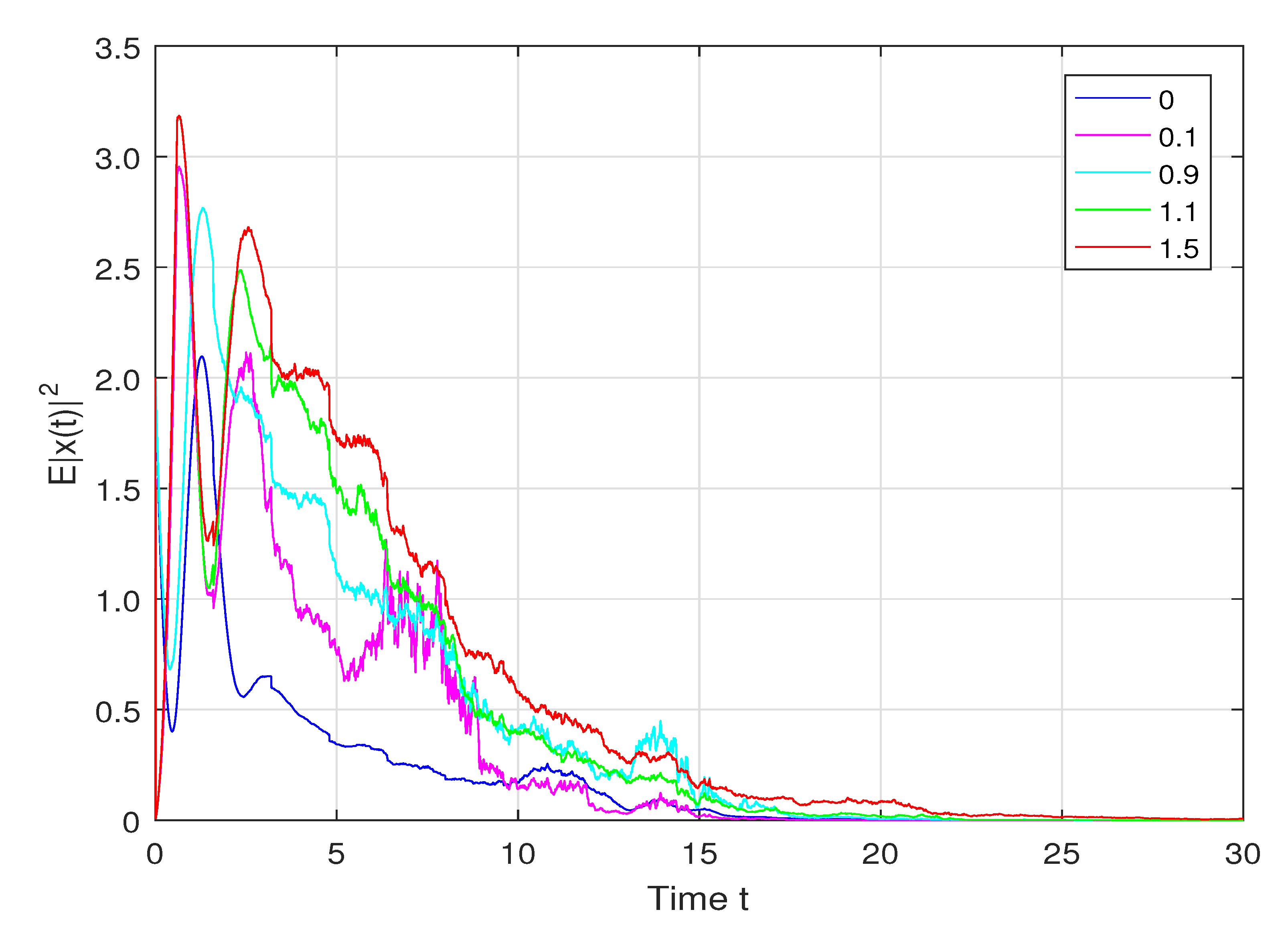
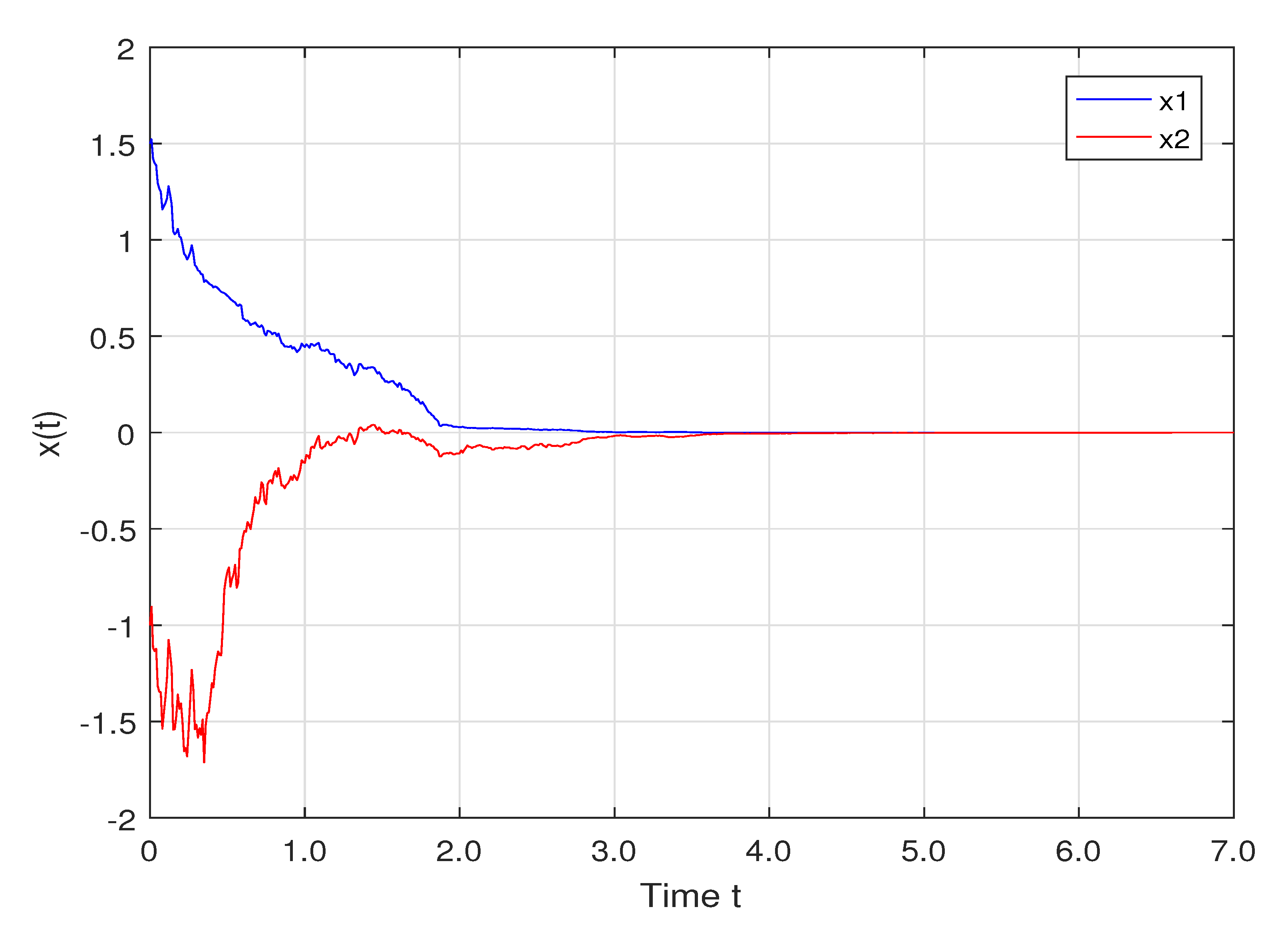
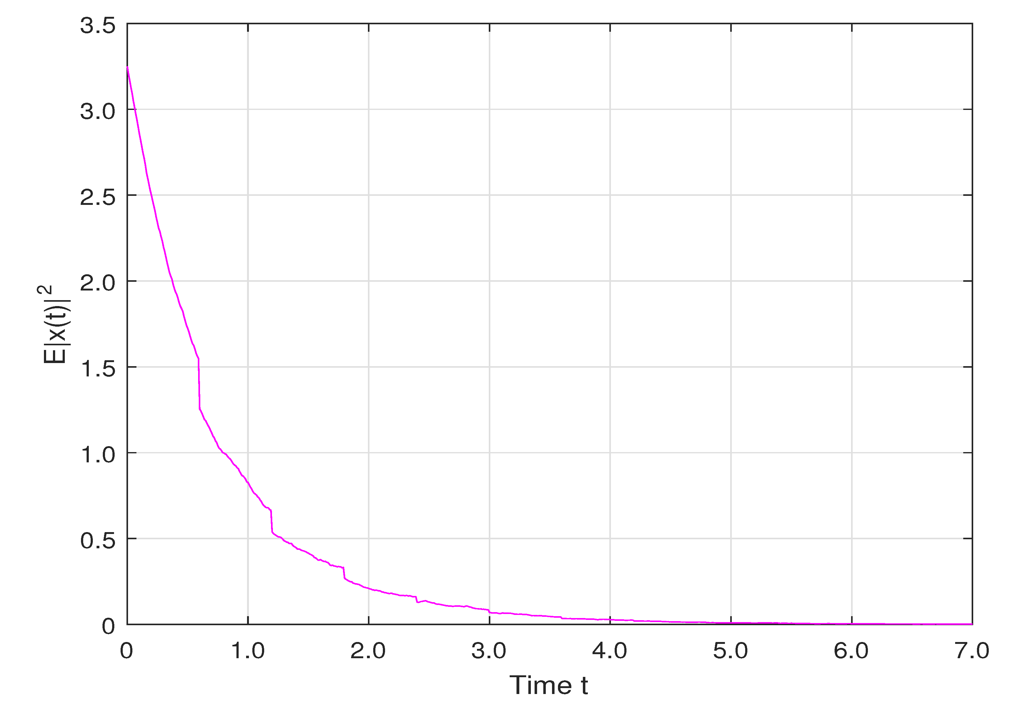
4. Examples

This section focuses on two numerical cases, which demonstrate the effectiveness of the obtained conclusions by simulations.

Example 1.

Consider the following linear ISDS:

$$\left\{\begin{array}{c}dx\left(t\right)=A_{1}x(t-{\tau }_1)dt+B_{1}x(t-{\delta }_1)dw\left(t\right),t\ne t_k,\hfill \\ \Delta x\left(t_k\right)=Cx\left(t_k^{-}\right),t_0=0,k\in {\mathbb{N}}^{+}\hfill \end{array}\right.$$

(28)

with

$$A_1=\left[\begin{array}{cc}-0.9& 0\\ 0.1& -0.47\end{array}\right],B_1=\left[\begin{array}{cc}0.39& 0.19\\ 0.36& -0.45\end{array}\right],C=-0.1I.$$

In (28), $x\left(t\right)={\left[x_1^T\left(t\right)x_2^T\left(t\right)\right]}^T$, ${\tau }_1=0.17$, ${\delta }_1=0.15$ and the impulsive switching time sequence meets $t_{k+1}=0.6+t_k$, $t_0=0$, $k\in {\mathbb{N}}^{+}$. By using the Matlab toolbox, it is clear that (28) satisfies the conditions of Theorem 1 with the feasible solutions below:

$$\begin{array}{cc}\hfill & P=\left[\begin{array}{cc}21.6495& -0.1601\\ -0.1601& 21.8271\end{array}\right],G_1=\left[\begin{array}{cc}3.6932& 1.7912\\ 1.7912& 8.0269\end{array}\right],W_{11}=\left[\begin{array}{cc}26.1435& -6.7963\\ -6.7963& 8.8955\end{array}\right],\hfill \\ \hfill & Q=\left[\begin{array}{cc}6.1923& 0.5685\\ 0.5685& 4.2735\end{array}\right],M_1=\left[\begin{array}{cc}11.255& -0.4153\\ -0.2828& 18.0384\end{array}\right],M_2=\left[\begin{array}{cc}12.1046& 1.509\\ -0.9563& 11.2162\end{array}\right],\hfill \\ \hfill & {\xi }_1=21.516,{\xi }_2=12.6316,\alpha =0.295,\beta =0.5,\gamma =0.08,\sigma =0.6.\hfill \end{array}$$

According to the above analysis, (28) satisfies the conditions of Theorem 1. Then, based on Euler-Maruyama method, Figure 1 and Figure 2 are plotted by MATLAB. Specifically, Figure 1 simulates the states trajectories of (28) with the initial function $\varphi \left(\theta \right)={[1.5-1]}^T$, $\theta \in [-0.17,0]$. And Figure 2 pictures the response of the mean square value of the system states (for the requirement of simulation, we let ${\mathbb{E}\left|x\left(t\right)\right|}^2=\frac{1}{1000}{\sum }_{s=1}^{1000}\left[\right|x_1^s{\left(t\right)|}^2+|x_2^s\left(t\right){|}^2]$, in which $x_k^s\left(t\right)$ is the sth sample path of $x_k\left(t\right)$, that is, the mean square value of the system states at each moment is obtained by taking the average of the values of 1000 sample paths). Obviously, in this numerical example, the simulation results show that the system is exponentially stable in the mean square sense, which verifies the validity of Theorem 1.

Figure 1. State trajectories of Example 1.

Figure 2. The curve of mean-square of 1000 paths with impulses.

Example 2.

Consider (28) with the following parameters:

$$\begin{array}{cc}\hfill & A_1=\left[\begin{array}{cc}-1& 1.6\\ 0.2& -0.7\end{array}\right],B_1=\left[\begin{array}{cc}0.4& 0.3\\ 0.4& -0.45\end{array}\right],\hfill \\ \hfill & C=-0.04I,t_{k+1}=1.6+t_k,k\in {\mathbb{N}}^{+}.\hfill \end{array}$$

Based on Theorem 2, one obtains that the maximum value of ${\tau }_1$ which ensures the stability is ${\tau }_1=0.6$. Taking ${\tau }_1=0.6$, by using the Matlab toolbox, it is clear that (28) satisfies the conditions of Theorem 2 with the feasible solutions below:

$$\begin{array}{cc}\hfill & P={10}^3\times \left[\begin{array}{cc}0.5150& -0.8018\\ -0.8018& 2.8934\end{array}\right],G_1={10}^3\times \left[\begin{array}{cc}0.6224& -0.8332\\ -0.8332& 3.7489\end{array}\right],\hfill \\ \hfill & W_{11}={10}^3\times \left[\begin{array}{cc}0.2612& -0.5438\\ -0.5438& 1.2359\end{array}\right],M_1={10}^3\times \left[\begin{array}{cc}0.5473& -0.7114\\ -0.7866& 2.9352\end{array}\right],\hfill \\ \hfill & M_2={10}^3\times \left[\begin{array}{cc}0.5765& 0.2234\\ -0.4054& 2.5864\end{array}\right].\hfill \end{array}$$

Letting ${\delta }_1=0,0.1,0.9,1.1,1.5,$ the curves of ${\mathbb{E}\left|x\left(t\right)\right|}^2$ with the corresponding ${\delta }_1$ are drew in Figure 3 under the same initial condition $\varphi \left(\theta \right)={[1-1]}^T$, $\theta \in [-\tau ,0],\tau =max\{{\tau }_1,{\delta }_1\}$. That is, the trajectories of the mean square value of the system states with the same drift term delay but different diffusion term delay are plotted in Figure 3. By comparing the trajectories, one obtains that although the systems with different diffusion term delays converge to 0 at different rates, it is seen that the systems are all mean-square stable, which verifies the feasibility of Theorem 2.

Figure 3. The curve of mean-square for different ${\delta }_1$.

5. Conclusions

In this paper, an appropriate LKF is displayed under the stochastic framework to set up the delay-dependent stability criterion for ISDSs. The sufficient conditions of exponential mean-square stability are presented in terms of LMIs. Meanwhile, in Example 1, when the system satisfies the conditions of Theorem 1, the trajectory of the mean square values of the system states plotted in Figure 2 shows the stability of the system. In particular, when mean-square stability is considered, we obtain the draft-delay-dependent/diffusion-delay-independent stability conditions, and such a conclusion is useful for systems with difficulties in measuring the time-delays of the diffusion term. Moreover, in Example 2, Figure 3 plots the corresponding trajectories of the system with different diffusion term delays, showing that diffusion term delays do not affect the mean-square stability of the system when the condition of Theorem 2 is satisfied, which verifies the validity of the theoretical results. In the future, we would like to apply the obtained stability theory to real systems. In addition, inspired by [30,31], we will further investigate the problems of estimation of system states and the design of controllers with multiple uncertainties using metaheuristic learning algorithms.

References

- Gu, K.; Kharitonov, V.L.; Chen, J. Stability of Time-Delay Systems; Birkhäuser: Boston, MA, USA, 2003. [Google Scholar]
- Wang, H.; Zhang, H.; Xie, L. Optimal control and stabilization for It systems with input delay. J. Syst. Sci. Complex. 2021, 34, 1895–1926. [Google Scholar] [CrossRef]
- Yan, S.; Shen, M.; Nguang, S.K.; Zhang, G. Event-triggered H∞ control of networked control systems with distributed transmission delay. IEEE Trans. Autom. Control 2020, 65, 4295–4301. [Google Scholar] [CrossRef]
- Lin, H.; Zeng, H.; Wang, W. New Lyapunov-Krasovskii functional for stability analysis of linear systems with time-varying delay. J. Syst. Sci. Complex. 2021, 34, 632–641. [Google Scholar] [CrossRef]
- Shi, J.; Wang, G. A non-zero differential game of BSDE with time-delayed generator with applications. IEEE Trans. Autom. Control 2016, 61, 1959–1964. [Google Scholar] [CrossRef]
- Ni, Y.; Yiu, C.; Zhang, H.; Zhang, J. Delayed optimal control of stochastic LQ problem. SIAM J. Control Optim. 2017, 55, 3370–3407. [Google Scholar] [CrossRef] [Green Version]
- Emilia, F. Introduction to Time-Delay Systems: Analysis and Control; Birkhäuser: Basel, Switzerland, 2014. [Google Scholar]
- Yan, H.; Tian, Y.; Li, H.; Zhang, H.; Li, Z. Input-output finite-time mean square stabilisation of nonlinear semi-Markovian jump systems with time-varying delay. Automatica 2019, 104, 82–89. [Google Scholar] [CrossRef]
- Feng, W.; Xie, Y.; Luo, F.; Zhang, X.; Duan, W. Enhanced stability criteria of network-based load frequency control of power systems with time-varying delays. Energies 2021, 14, 5820. [Google Scholar] [CrossRef]
- Chen, W.; Wang, Z.; Lu, X. Delay-dependent exponential stability of uncertain stochastic systems with multiple delays: An LMI approach. Syst. Control Lett. 2005, 54, 547–555. [Google Scholar] [CrossRef]
- Yue, D.; Han, Q. Delay-dependent exponential stability of stochastic systems with time-varying delays, nonlinearities and Markovian jump parameters. IEEE Trans. Autom. Control 2005, 50, 217–222. [Google Scholar]
- Luo, S.; Deng, F. A note on delay-dependent stability of It-type stochastic time-delay systems. Automatica 2019, 105, 443–447. [Google Scholar] [CrossRef]
- Tunç, O.; Tunç, C.; Wang, Y. Delay-dependent stability, integrability and boundedeness criteria for delay differential systems. Axioms 2021, 10, 138. [Google Scholar] [CrossRef]
- Lakshmikantham, V. Theory of Impulsive Differential Equations; World Scientific: Singapore, 1989. [Google Scholar]
- Samoilenko, A.M.; Perestyuk, N.A. Impulsive Differential Equations; World Scientific: Singapore, 1995. [Google Scholar]
- Chen, W.; Zheng, W. Exponential stability of nonlinear time-delay systems with delayed impulse effects. Automatica 2011, 47, 1075–1083. [Google Scholar] [CrossRef]
- Peng, S.; Deng, F.; Zhang, Y. A unified Razumikhin-type criterion on input-to-state stability of time-varying impulsive delayed systems. Syst. Control Lett. 2018, 45, 20–28. [Google Scholar] [CrossRef]
- Ren, W.; Xiong, J. Stability analysis of impulsive switched time-delay systems with state-dependent impulses. IEEE Trans. Autom. Control 2019, 64, 3928–3935. [Google Scholar] [CrossRef]
- Xu, S.; Chen, T. Robust H∞ filtering for uncertain impulsive stochastic systems under sampled measurements. Automatica 2003, 39, 509–516. [Google Scholar] [CrossRef]
- Mohamad, S.A.; Liu, X.; Xie, W. Existence, continuation, and uniqueness problems of stochastic impulsive systems with time delay. J. Frankl. Inst. 2010, 347, 1317–1333. [Google Scholar]
- Cheng, P.; Deng, F. Global exponential stability of impulsive stochastic functional differential systems. Stat. Probab. Lett. 2010, 80, 1854–1862. [Google Scholar] [CrossRef]
- Zhu, Q. pth moment exponential stability of impulsive stochastic functional differential equations with Markovian switching. J. Frankl. Inst. 2014, 351, 3965–3986. [Google Scholar] [CrossRef]
- Pan, L.; Cao, J.; Ren, Y. Impulsive stability of stochastic functional differential systems driven by G-Brownian motion. Mathematics 2020, 8, 227. [Google Scholar] [CrossRef] [Green Version]
- Ngoc, P.; Hieu, L. A novel approach to mean square exponential stability of stochastic delay differential equations. IEEE Trans. Autom. Control. 2020, 66, 2351–2356. [Google Scholar] [CrossRef]
- Yang, J.; Zhong, S.; Luo, P. Mean square stability analysis of impulsive stochastic differential equations with delays. J. Comput. Appl. Math. 2008, 216, 474–483. [Google Scholar] [CrossRef] [Green Version]
- Zhu, Q.; Song, B. Exponential stability of impulsive nonlinear stochastic differential equations with mixed delays. Nonlinear Anal. Real World Appl. 2011, 12, 2851–2860. [Google Scholar] [CrossRef]
- Rami, M.A.; Zhou, X. Linear matrix inequalities, Riccati equations, and indefinite stochastic linear quadratic controls. IEEE Trans. Autom. Control 2000, 45, 1131–1143. [Google Scholar] [CrossRef]
- Mao, X. Stochastic Differential Equations and Applications, 2nd ed.; Howrwood Publishing: Chichester, UK, 2007. [Google Scholar]
- Emilia, F. New Lyapunov-Krasovskii functionals for stability of linear retarded and neutral type systems. Syst. Control Lett. 2001, 43, 309–319. [Google Scholar]
- Yang, G.; Yao, J.; Dong, Z. Neuroadaptive learning algorithm for constrained nonlinear systems with disturbance rejection. Int. J. Robust Nonlinear Control 2022, 32, 6127–6147. [Google Scholar] [CrossRef]
- Yang, G.; Yao, J.; Ullah, N. Neuroadaptive control of saturated nonlinear systems with disturbance compensation. ISA Trans. 2022, 122, 49–62. [Google Scholar] [CrossRef]
Publisher’s Note: MDPI stays neutral with regard to jurisdictional claims in published maps and institutional affiliations. |
© 2022 by the authors. Licensee MDPI, Basel, Switzerland. This article is an open access article distributed under the terms and conditions of the Creative Commons Attribution (CC BY) license (https://creativecommons.org/licenses/by/4.0/).
Share and Cite
Xiao, C.; Hou, T. Delay-Dependent Stability of Impulsive Stochastic Systems with Multiple Delays. Processes 2022, 10, 1258. https://doi.org/10.3390/pr10071258
Xiao C, Hou T. Delay-Dependent Stability of Impulsive Stochastic Systems with Multiple Delays. Processes. 2022; 10(7):1258. https://doi.org/10.3390/pr10071258
Chicago/Turabian StyleXiao, Chunjie, and Ting Hou. 2022. "Delay-Dependent Stability of Impulsive Stochastic Systems with Multiple Delays" Processes 10, no. 7: 1258. https://doi.org/10.3390/pr10071258
APA StyleXiao, C., & Hou, T. (2022). Delay-Dependent Stability of Impulsive Stochastic Systems with Multiple Delays. Processes, 10(7), 1258. https://doi.org/10.3390/pr10071258