Frequency Domain Analysis of Fluid–Structure Interaction in Aircraft Hydraulic Pipe with Complex Constraints

Abstract

This paper focuses on the frequency domain fluid–structure interaction (FSI) vibration characteristics of aircraft hydraulic pipe with complex constraints. The linear partial differential fourteen-equation model is applied to describe the nonlinear FSI dynamics of pipes conveying fluid with high-speed, high-pressure, a wide Reynolds number, and the vibration frequency range. The excitation, complex boundary, and middle constraint models of liquid-filled pipes are analytically established and added into the global model of the pipe system. These resulting models are solved by the improved Laplace transform transfer matrix method (LTTMM) in the frequency domain. Then, the dynamic response characteristics of an aircraft hydraulic pipe containing diverse constraints are investigated numerically and experimentally under four types of working conditions, and the improvement conditions for the numerical instabilities are presented. In general, the present method is highly efficient and convenient for rapid model parameter modifications, in order to be fully applicable to different pipe systems and analysis cases. The results reveal the complex resonant laws regarding aircraft hydraulic pipes with complex constraints in the broad frequency band, which can also provide theoretical reference and technical support for FSI vibration analysis and the control of aircraft hydraulic pipes.

1. Introduction

The frequency range and intensity of fluid fluctuations in aircraft hydraulic systems are widened and aggravated due to high-velocity and -pressure conditions, and the vibration modes of aircraft hydraulic pipes are diverse, on account of the complex pipe structures or multiple structural supports, as well as a wide range of external excitations. The resulting fluid–structure interaction (FSI) vibration can easily cause pipe rupture and leakage failure, thus threatening the reliability of the hydraulic systems and safety of the aircraft. Therefore, it is a significant research work to investigate the frequency domain FSI vibration characteristics of aircraft hydraulic pipes.

Considerable research regarding the FSI nonlinear dynamics characteristics of aircraft hydraulic pipes has been reported in the past years [1,2,3,4,5,6,7,8,9,10,11,12]. The precondition for analyzing these dynamic behaviors was to establish an accurate mathematical model. Many researchers deduced the dynamics model for pipes conveying fluid, and linear partial differential equations were used for the relevant study in this paper. The typical existing research results and status are summarized. Skalak [13] defined the fundamental four-equation model as describing the axial vibration of pipes conveying fluid, where the water hammer model was coupled to two equations regarding the axial force model for the pipe; the friction and damping effects were disregarded. Then, by considering Poisson coupling and factors for the pipe wall thickness, the four-equation model was further modified and extended by Wiggert et al. and Tijsseling [14,15] to have smaller correction terms, and it achieved good predictions of a straight single pipe in a pipe system [16]. Based on the theory of inviscid compressible fluid pressure pulses in a thin-walled pipe, Walker and Phillips [17] developed the six-equation model, and it was applied to the numerical solution of a water-filled copper pipe with a cap under an axial impulsive force. The eight-equation model, used to describe plane elbow, was first proposed by Davidson and Smith [18] and includes four axial vibration equations and four transverse vibration equations. Gale and Tiselj [19] improved Skalak’s four-equation model by adding four Timoshenko’s beam equations and presented the eight-equation model for the description of the two-way fluid–structure interaction of both one-dimensional pipes and two-dimensional planar pipes with arbitrary shape; this model was successfully applied to the numerical simulation of the tank–pipe–valve system. Wilkinson [20] proposed the fourteen-equation model based on the Bernoulli–Euler beam model, and transfer matrices and equations representing boundary various conditions were derived. Then, the fourteen-equation model was extended and widely used by many scholars [21,22,23,24] for modelling fluid pulsation, Poisson coupling, friction coupling, junction coupling, deformation of the pipe in various directions, extra mass, springs, and various complex boundary conditions. Moreover, the fourteen-equation model has been applied to the analysis of some complex engineering environments [1,4,10,23,25], and it has become the most systemic model at present. Notably, Tan et al. [26] found that Timoshenko beam theory is more suitable for studying the vibration characteristics of pipes conveying high-speed fluid. Therefore, the engineering application and verification of the fourteen-equation model based on Timoshenko beam theory in high-speed fluid transmission pipes deserve further study.

In the above-mentioned models, only semi-analytical or numerical methods can be used for solving; the representative methods are as follows: method of characteristics (MOC) [14,27,28,29,30], finite element method (FEM) [31,32,33], MOC–FEM [34,35], and transfer matrix method (TMM) [1,4,10,21,23,24,25,36,37,38,39]. MOC and MOC–FEM are especially used for fluid transient response analysis in the time domain, while FEM and TMM are widely used for forced vibration response in the frequency domain [1]. FEM is the most common method for analyzing complex pipe structures; however, FEM requires a better quality mesh to ensure solution precision at high frequencies [3], which will consume a lot of computing time and memory resources [36]. Compared with FEM, the TMM can not only construct the governing equation more easily, but it can also lessen the amount of calculation; therefore, the TMM is easily adaptable to industrial applications. The typical existing research works are summarized. Considering straight and uniformly curved tubing segments as a one-dimensional distributed parameter system, Tentarelli [21] proposed an appropriate set of dynamic models and analytical methods that were applicable to simple sections and complex pipe systems, and they were based on the TMM. Lesmez et al. [39] deduced the overall transfer matrix of the pipe system conveying fluid; the corresponding state vectors of the pipe and fluid were provided, and the modal analysis of pipe was carried out and verified. By comparing the difference between the direct numerical analysis in frequency domain and frequency domain results obtained from the time domain via Laplace transform, Zhang and Tijsseling et al. [38] proposed a frequency domain solution method based on the Laplace transform transfer matrix method (LTTMM) and verified by the typical tests designed by Dundee University and Delft Hydraulic Research Institute. Xu et al. [24] used the fourteen-equation model to describe the FSI in liquid-filled complex pipelines and proposed a general solution method to predict the frequency response of multi-branch pipes based on the transfer matrix method. A series of theoretical research was carried out by the Harbin Engineering University research team [23,36,37,40]. A transfer matrix method in the frequency domain that considered the FSI of the liquid-filled pipes with elastic constraints was proposed by using the point transfer matrix. The fluid pressure and vibrations of branched pipes were analyzed based on an absorbing transfer matrix method in the frequency domain. The application range of various types of models and simulation algorithms of fluid-filled pipe systems that considered the FSI in the frequency domain were compared and discussed. Based on the transfer matrix method, the Yanshan University research team [1,4,10,25] carried out theoretical research and experimental verification of FSI vibration of aircraft hydraulic pipes, which broadens the application range of the transfer matrix method in engineering practice. From the above review, it can be seen that TMM has been widely used in the vibration problems of pipes conveying fluid, due to its good adaptability, compared with other solution methods.

The aforementioned studies dealt with mathematical models and analysis methods that are sufficient to handle the FSI dynamics of simple fluid-conveying pipe systems, and the constraints are limited only to simple excitation and boundary conditions. More extensive mathematical models for a wide range of fluid pressures, Reynolds numbers, and the wide-range vibration frequencies of the structures (the constraints of which can describe arbitrary excitation and boundary conditions) deserve further investigation. In addition, as a calculation method applicable to cascaded structures, the TMM requires the assembly of multiple matrix cells. The calculation cases of complex pipes for directing practice in the engineering field and problem of overflow in the calculation and calculation result instability in high-frequency ranges need to be further discussed.

The present work developed a more comprehensive FSI governing the equations of three-dimensional space pipes conveying fluid. The excitation, complex boundary, and middle constraint models were established and added into the global model of the pipe system. Further, the unified expression of the improved Laplace transform transfer matrix method (LTTMM) for solving the FSI governing the equations was derived, forming the frequency methodology to solve for hydraulic pipe systems containing diverse constraints. Then, the frequency domain FSI response of an aircraft hydraulic pipeline containing diverse constraints under various cases was analyzed through numerical and experimental methods, and the results reveal the complex resonant laws regarding aircraft hydraulic pipes with complex constraints in the broad frequency band and prove the accuracy and efficiency of the presented method.

2. Theoretical Modeling

2.1. FSI Fourteen-Equation Model

An aircraft hydraulic pipe is thin-walled and slender, with wide vibration frequency and large fluid velocity in the pipe, which is more suitable for simulation via Timoshenko beam theory. Fourteen partial differential equations that describe the pipe conveying fluid (Figure 1) were established based on the acoustic wave equation and Timoshenko beam dynamic model, which describe the fluid dynamics and axial/flexural/torsional motions of the pipe in three-dimensional space, thus basically containing two equations of fluid motion and three sets of twelve equations of pipe motion. The fundamental assumptions and applicable conditions of the governing equations refer to the published literature [1].

• The axial motion.

  $$\frac{\partial V_f}{\partial t}+V\frac{\partial V_f}{\partial l}+\frac{1}{{\rho }_f}\frac{\partial P}{\partial l}+\frac{4}{{\rho }_{f}D}{\tau }_w+g\sin \beta =0$$

  (1)

  $$\frac{\partial {\dot{w}}_z}{\partial t}+\frac{1}{{\rho }_p{A}_p}\frac{\partial f_z}{\partial l}+\frac{1}{{\rho }_p{A}_p}\frac{f_y}{R_p}-\frac{4}{{\rho }_p{A}_p{\rho }_{f}D}{\tau }_w+g\sin \beta -\frac{f_{ez}}{{\rho }_p{A}_p}=0$$

  (2)

  $$\frac{\partial P}{\partial t}-2v{K}^{\prime }\frac{\partial {\dot{w}}_z}{\partial l}+K^{\prime }\frac{\partial V_f}{\partial l}+K^{\prime }(1-2v)\frac{{\dot{w}}_y}{R_w}=0$$

  (3)

  $$\frac{\partial f_z}{\partial t}+\left[E{A}_p+\frac{4v^2{K}^{\prime }{A}_p}{e_R\left(2+e_R\right)}\right]\frac{\partial {\dot{w}}_z}{\partial l}-\frac{2v{K}^{\prime }{A}_p}{e_R\left(2+e_R\right)}\frac{\partial V_f}{\partial l}+\left[E{A}_p+\frac{2v(1-2v)K^{\prime }{A}_p}{e_R\left(2+e_R\right)}\right]\frac{{\dot{w}}_y}{R_p}=0$$

  (4)
• The flexural motion in the x-z plane.

  $$\frac{\partial M_y}{\partial t}+E{I}_p\frac{\partial {\dot{\theta }}_y}{\partial l}-E{I}_p\frac{{\dot{\theta }}_z}{R_p}=0$$

  (5)

  $$\frac{\partial {\dot{w}}_x}{\partial t}+\frac{1}{m}\frac{\partial f_x}{\partial l}-\frac{2m_{f}V}{m}\frac{\partial {\dot{w}}_x}{\partial l}-\frac{m_f{V}^2+P{A}_f}{m}\left(\frac{1}{E{I}_p}{M}_y-\frac{{\theta }_z}{R_p}\right)+g\cos \beta -\frac{1}{m}{f}_{ex}=0$$

  (6)

  $$\frac{\partial f_x}{\partial t}+\kappa G{A}_p\frac{\partial {\dot{w}}_x}{\partial l}-\kappa G{A}_p{\dot{\theta }}_y=0$$

  (7)

  $$\frac{\partial {\dot{\theta }}_y}{\partial t}+\frac{1}{T_y}\frac{\partial M_y}{\partial l}+\frac{1}{T_y}{f}_x-\frac{1}{T_y{R}_p}{M}_z-\frac{1}{T_y}{M}_{ey}=0$$

  (8)
• The flexural motion in y-z plane.

  $$\frac{\partial M_x}{\partial t}+E{I}_p\frac{\partial {\dot{\theta }}_x}{\partial l}=0$$

  (9)

  $$\frac{\partial {\dot{w}}_y}{\partial t}+\frac{1}{m}\frac{\partial f_y}{\partial l}+\frac{2m_{f}V}{m}\frac{\partial {\dot{w}}_y}{\partial l}+\frac{m_f{V}^2+P{A}_f}{m}\left(\frac{M_x}{E{I}_p}-\frac{1}{R_p}\right)-\frac{1}{m{R}_p}{f}_z+g\cos \beta -\frac{1}{m}{f}_{ey}=0$$

  (10)

  $$\frac{\partial f_y}{\partial t}+\kappa G{A}_p\frac{\partial {\dot{w}}_y}{\partial l}+\kappa G{A}_p{\dot{\theta }}_x-\frac{\kappa G{A}_p}{R_p}{\dot{w}}_z=0$$

  (11)

  $$\frac{\partial {\dot{\theta }}_x}{\partial t}+\frac{1}{T_x}\frac{\partial M_x}{\partial l}-\frac{1}{T_x}{f}_y-\frac{1}{T_x}{M}_{ey}=0$$

  (12)
• The torsional motion about z axis.

  $$\frac{\partial M_z}{\partial t}+G{J}_p\frac{\partial {\dot{\theta }}_z}{\partial l}+\frac{G{J}_p}{R_p}{\dot{\theta }}_y=0$$

  (13)

  $$\frac{\partial {\dot{\theta }}_z}{\partial t}+\frac{1}{{\rho }_p{J}_p}\frac{\partial M_z}{\partial l}+\frac{1}{{\rho }_p{J}_p{R}_p}{M}_y-\frac{1}{{\rho }_p{J}_p}{M}_{ez}=0$$

  (14)

  in Equation (2)

  $${\tau }_w={\tau }_{ws}+{\tau }_{wuz}+{\tau }_{wub}=\frac{\rho fV\left|V\right|}{8}+k\frac{4\rho V}{D}{\displaystyle {\int }_0^t\frac{\partial V\left(t\right)}{\partial t}\frac{C_1{e}^{-C_{2}t}}{\sqrt{\pi t}}dt}+(1-k)\frac{\rho D}{4}\cdot k_3\left(\frac{\partial V}{\partial t}-\alpha \frac{\partial V}{\partial z}\right)$$

  (15)

  where ${\tau }_{ws}$ represents the wall shear friction in steady flow; ${\tau }_{wuz}$ and ${\tau }_{wub}$, respectively, denote the Zielke and Brunone additional wall shear friction in unsteady flow. Note that, at this point, the selection coefficient k is set to 1 when the flow form has transient laminar flow or low-Reynolds-number turbulence (Re < 2320); instead, k is set to 0 when the flow form has unsteady turbulence and high-Reynolds-number turbulence (Re > 2320) [4]. Accordingly, the following parameters are introduced:

  $$C_1=\frac{R}{2\sqrt{v_w}},C_2=\frac{0.135v_w}{R^2}R{e}^{k_4}$$

  (16)

  $$k_3=\sqrt{\frac{7.41/R{e}^{k_4}}{2}},k_4=\lg (14.3/R{e}^{0.05})$$

  (17)

  $$\alpha =\frac{\sqrt{K/{\rho }_f}}{\sqrt{1+DK/eE}}$$

  (18)

Fourteen system variables in the above Equations (1)–(14) could be written as a state vector:

$$\mathsf{\Phi }(z,t)={\left[V P {\dot{w}}_z f_z M_y {\dot{\theta }}_y {\dot{w}}_x f_x M_x {\dot{\theta }}_x {\dot{w}}_y f_y {\dot{\theta }}_z M_z\right]}^T$$

(19)

Then, the matrix expression of the fourteen equations can be expressed as:

$$\mathbf{A}\frac{\partial \mathsf{\Phi }(z,t)}{\partial t}+\mathbf{B}\frac{\partial \mathsf{\Phi }(z,t)}{\partial z}+\mathbf{C}\mathsf{\Phi }(z,t)+\mathbf{D}=\mathbf{y}(z,t)$$

(20)

Here, A, B, and C are coefficient matrices within the dimensional scales of 14 multiplied by 14. A and B are the constant terms of time and space differentiation, respectively. C and D are coefficient matrices, including friction and viscous damping and gravity, respectively; vector y describes the external excitation.

2.2. Boundary and Excitation Model

In the practical piping system, there are complex excitations, boundary conditions, and pipeline supports. Establishing accurate constraints model is a very crucial step for solving the dynamic equations of the pipe conveying fluid. Referring to the fundamental ideas in [24], pipe constraints mainly include external excitations (fluid excitation, mechanical shock, and simple harmonic vibration), boundary conditions (pipe end closure, velocity boundary, and pressure boundary), and the middle constraints that exist at the positions of the supports. The constraint modeling with the time domain method has been presented by the authors [1]—that, in the frequency domain, will be discussed in this section. It should be noted that the method proposed here for complex excitations can also be used in pipe systems, not just for a single pipe.

For the boundary at both ends of the pipe, it can be assumed that there exists a virtual mechanical node between the external excitation and pipe ends, which have a force balance relationship and motion continuity. The force balance and local coordinate systems for the boundary nodes at the ends of the pipe are shown in Figure 2, supposing one node as the analysis object, where $F_x$, $F_y$, and $F_z$ are constraint forces (including inertial force) in three directions, respectively, $T_x$, $T_y$, and $T_z$ are constraint moments, and $F_r$ is the external excitation. Additionally, if the actual pipe is an open end, the fluid force $A_{f}P$ will be ignored, and the extra mass of the node needs to be considered, in case the pipe ends with lumped mass.

For the fourteen-equation model, there are seven boundary equations at each pipe end, and the corresponding excitation vectors can be written as:

$$\{\begin{array}{l}{\left[{\mathbf{Q}}_0\left(s\right)\right]}_{7\times 1}={\left[\begin{array}{ccccccc}V(0,s)& f_{ez}(0,s)& f_{ex}(0,s)& M_{ey}(0,s)& f_{ey}(0,s)& M_{ex}(0,s)& M_{ez}(0,s)\end{array}\right]}^{\mathrm{T}}\\ {\left[{\mathbf{Q}}_L\left(s\right)\right]}_{7\times 1}={\left[\begin{array}{ccccccc}V(L,s)& f_{ez}(L,s)& f_{ex}(L,s)& M_{ey}(L,s)& f_{ey}(L,s)& M_{ex}(L,s)& M_{ez}(L,s)\end{array}\right]}^{\mathrm{T}}\end{array}$$

(21)

The above formula indicates that the first element of each vector is fluid excitation, and the other six elements correspond to the force and moment equations of three motion planes, respectively.

According to Equation (36), the boundary matrices of two pipe ends can be defined correspondingly. Then, the boundary matrices of the closed ends, considering elastic restraint, extra mass, and inertia, can be written as:

$${\mathbf{D}}_0(s)=\left[\begin{array}{cccccccccccccc}1& 0& -1& 0& 0& 0& 0& 0& 0& 0& 0& 0& 0& 0\\ 0& -A_f& -K_{z(0)}& 1& 0& 0& 0& 0& 0& 0& 0& 0& 0& 0\\ 0& 0& 0& 0& 1& -T_{y(0)}& 0& 0& 0& 0& 0& 0& 0& 0\\ 0& 0& 0& 0& 0& 0& -K_{x(0)}& 1& 0& 0& 0& 0& 0& 0\\ 0& 0& 0& 0& 0& 0& 0& 0& 1& -T_{x(0)}& 0& 0& 0& 0\\ 0& 0& 0& 0& 0& 0& 0& 0& 0& 0& -K_{y(0)}& 1& 0& 0\\ 0& 0& 0& 0& 0& 0& 0& 0& 0& 0& 0& 0& -T_{z(0)}& 1\end{array}\right]$$

(22)

$${\mathbf{D}}_L(s)=\left[\begin{array}{cccccccccccccc}1& 0& -1& 0& 0& 0& 0& 0& 0& 0& 0& 0& 0& 0\\ 0& -A_f& K_{z(0)}& 1& 0& 0& 0& 0& 0& 0& 0& 0& 0& 0\\ 0& 0& 0& 0& 1& K_{y(0)}& 0& 0& 0& 0& 0& 0& 0& 0\\ 0& 0& 0& 0& 0& 0& T_{x(0)}& 1& 0& 0& 0& 0& 0& 0\\ 0& 0& 0& 0& 0& 0& 0& 0& 1& K_{x(0)}& 0& 0& 0& 0\\ 0& 0& 0& 0& 0& 0& 0& 0& 0& 0& T_{y(0)}& 1& 0& 0\\ 0& 0& 0& 0& 0& 0& 0& 0& 0& 0& 0& 0& T_{z(0)}& 1\end{array}\right]$$

(23)

where

$$\{\begin{array}{l}{K}_{x(i)}=\frac{k_{x(i)}}{s}+m_{c(i)}s,K_{y(j)}=\frac{k_{y(i)}}{s}+m_{c(i)}s,K_{z(j)}=\frac{k_{z(i)}}{s}+m_{c(i)}s\\ T_{x(i)}=\frac{t_{x(i)}}{s},T_{y(i)}=\frac{t_{y(i)}}{s},T_{z(i)}=\frac{t_{z(i)}}{s}\end{array}$$

(24)

where $K_{(i)}$ and $T_{(i)}$ are linear velocity impedance and rotational angular velocity impedance coefficients, respectively. k, t, and m_c are the linear stiffness, torsional stiffness, and extra mass, respectively. For free or fixed support, the stiffness coefficients are set to zero or a large value, respectively; for elastic support, the values of each coefficient need to be set according to the specific constraints.

Given all of that, the complex boundary conditions and external excitations of the pipe can be characterized via modifying the first-row coefficient of the boundary matrix and first element of the excitation vector, so as to calculate the complex constraints at both pipe ends in the presented method.

2.3. Middle Constraint Model

As the most common configuration of hydraulic pipe systems, the cascaded pipe usually consists of a series of straight pipe sections and elbow units. Regarding the side pipes of the connection node as different pipe sections, the force balance and motion continuity of the node at the middle constraint are shown in Figure 3.

Based on the point transfer matrix method defined by TMM, the state vectors at both sides of the middle constraint node are provided:

$${\tilde{\mathsf{\Phi }}}_{i+1}(0,s)={\mathrm{N}}_i(s){\tilde{\mathsf{\Phi }}}_i(L_i,s)$$

(25)

where the middle constraint matrix ${\mathbf{N}}_i$ is provided as follows, which can describe as free, fixed, and other complex constraints by changing its impedance coefficients.

$${\mathbf{N}}_i=\left[\begin{array}{cccccccccccccc}1& 0& 0& 0& 0& 0& 0& 0& 0& 0& 0& 0& 0& 0\\ 0& 1& 0& 0& 0& 0& 0& 0& 0& 0& 0& 0& 0& 0\\ 0& 0& 1& 0& 0& 0& 0& 0& 0& 0& 0& 0& 0& 0\\ 0& 0& K_{zi}& 1& 0& 0& 0& 0& 0& 0& 0& 0& 0& 0\\ 0& 0& 0& 0& 1& 0& 0& 0& 0& 0& 0& 0& 0& 0\\ 0& 0& 0& 0& 0& 1& 0& 0& 0& 0& 0& 0& 0& 0\\ 0& 0& 0& 0& 0& T_{yi}& 1& 0& 0& 0& 0& 0& 0& 0\\ 0& 0& 0& 0& 0& 0& K_{xi}& 1& 0& 0& 0& 0& 0& 0\\ 0& 0& 0& 0& 0& 0& 0& 0& 1& 0& 0& 0& 0& 0\\ 0& 0& 0& 0& 0& 0& 0& 0& 0& 1& 0& 0& 0& 0\\ 0& 0& 0& 0& 0& 0& 0& 0& 0& T_{xi}& 1& 0& 0& 0\\ 0& 0& 0& 0& 0& 0& 0& 0& 0& 0& K_{yi}& 1& 0& 0\\ 0& 0& 0& 0& 0& 0& 0& 0& 0& 0& 0& 0& 1& 0\\ 0& 0& 0& 0& 0& 0& 0& 0& 0& 0& 0& 0& T_{zi}& 1\end{array}\right]$$

(26)

Terms $K_{(i)}$ and $T_{(i)}$ are the linear velocity impedance and rotational angular velocity impedance, which are the same as those defined in Equations (24), and can be estimated via the finite element method or a test.

Note that, at this point, the middle constraint matrix represents the transfer relationship for the discontinuous character of the cascaded pipe (Figure 4), which is defined as a unit matrix when no constraints exist; the pipe areas are equal at the connections between the two pipe sections.

The global transfer matrix is proposed to solve the cascaded pipe with complex middle constraints, which can be derived by multiplying a series of related field and point transfer matrices.

$${\mathbf{U}}_{\mathrm{a}\mathrm{l}\mathrm{l}}(s)={\mathbf{U}}_N(L_N,s)\cdots {\mathbf{U}}_{i+1}(L_{i+1},s){\mathbf{N}}_i(s){\mathbf{U}}_i(L_i,s)\cdots {\mathbf{U}}_1(L_1,s)$$

(27)

The calculation procedures of ${\mathbf{N}}_i$ and ${\mathbf{U}}_{\mathrm{a}\mathrm{l}\mathrm{l}}(t_i)$, see Equations (35)–(40).

3. Laplace Transform Transfer Matrix Method

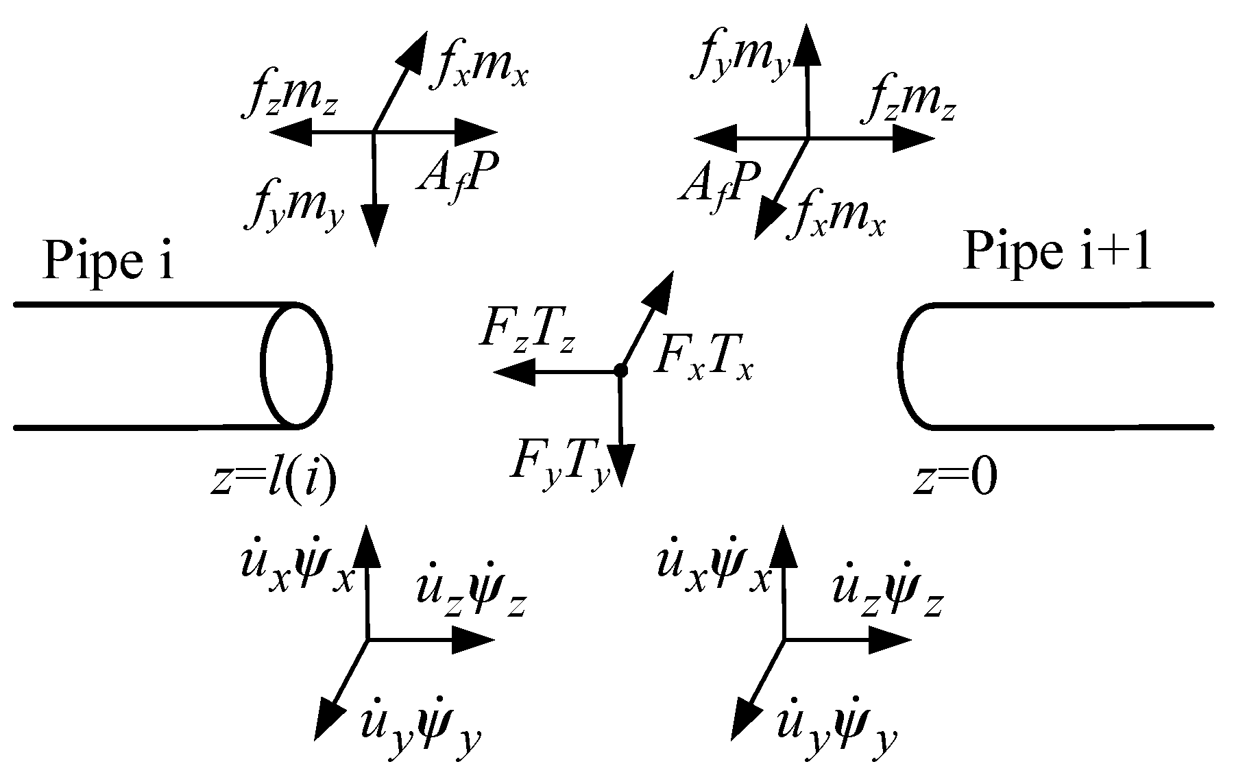
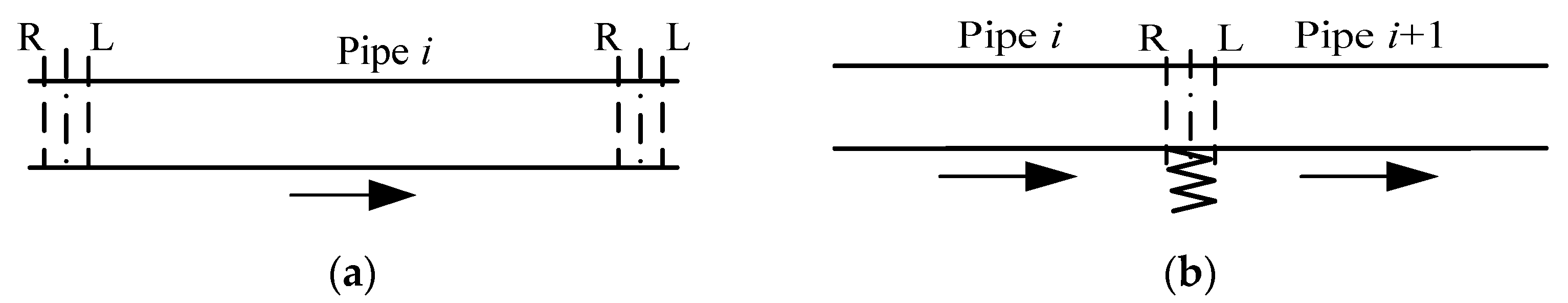
The TMM has been comprehensively applied to FSI analysis in piping systems. Figure 5 shows the state vectors and correlated matrix relations of the single pipe section and cascaded pipe with middle support.

The fourteen-equation model can be accurately solved in the frequency domain, and the LTMM for the fourteen partial differential equations is derived in this section; meanwhile, some improvements and expansions are also performed.

Equation (20) provides the matrix expression of the fourteen equations; then, let ${\mathbf{A}}^{*}=s\mathbf{A}+\mathbf{C}$, ${\mathbf{y}}^{*}(z,s)=\tilde{\mathbf{y}}(z,s)-\frac{1}{s}\mathbf{D}-{\mathbf{A}\mathsf{\Phi }(z,t)|}_{t=0}$. Equation (28) can be obtained via Laplace transform:

$$\tilde{\mathsf{\Phi }}(z,s)+{\mathbf{A}}^{*}{}^{-1}\mathbf{B}\frac{\partial \tilde{\mathsf{\Phi }}(z,s)}{\partial z}={\mathbf{A}}^{*}{}^{-1}{\mathbf{y}}^{*}(z,s)$$

(28)

where $\tilde{\mathsf{\Phi }}(z,s)={\displaystyle {\int }_0^{\infty }{e}^{-st}\mathsf{\Phi }(z,t)}dt$, $\tilde{\mathbf{y}}(z,s)={\displaystyle {\int }_0^{\infty }{e}^{-st}\mathbf{y}(z,t)dt}$.

$\tilde{\mathsf{\eta }}(z,s)={\mathbf{V}}^{-1}\tilde{\mathsf{\Phi }}(z,s)$, ${\tilde{\mathsf{\eta }}}_r(z,s)={\mathbf{V}}^{-1}{\mathbf{A}}^{-1}{\mathbf{y}}^{*}(z,s)$, Equation (28) can be simplified as:

$$\frac{\partial \tilde{\mathsf{\eta }}(z,s)}{\partial \mathrm{z}}+{\mathbf{T}}^{-1}\tilde{\mathsf{\eta }}(z,s)={\mathbf{T}}^{-1}{\tilde{\mathsf{\eta }}}_r(z,s)$$

(29)

where $\mathbf{T}=\mathrm{diag}\{{\lambda }_1(s),{\lambda }_2(s),\cdots {\lambda }_{14}(s)\}$ and $\mathrm{V}={[{\xi }_1(s) {\xi }_2(s) \cdots {\xi }_{14}(s)]}^{\mathrm{T}}$ are the eigenvalues and eigenvector of ${\mathbf{A}}^{*}{}^{-1}\mathbf{B}$, respectively.

Evidently, the linear ordinary differential Equation (29) can be solved as:

$$\tilde{\mathsf{\eta }}(z,s)=\mathbf{E}(z,s){\tilde{\mathsf{\eta }}}_0(s)+{\tilde{\mathsf{\eta }}}_r^{*}(z,s)$$

(30)

where

$$\{\begin{array}{l}\mathbf{E}(z,s)=\mathrm{diag}\{e(-sz/{\lambda }_1(s)),e(-sz/{\lambda }_2(s)),\cdots ,e(-sz/{\lambda }_{14}(s))\}\\ {\tilde{\mathsf{\eta }}}_r^{*}(z,s)=\left(\begin{array}{cccc}{\tilde{\eta }}_1(z,s)& {\tilde{\eta }}_2(z,s)& \cdots & {\tilde{\eta }}_{14}(z,s)\end{array}\right)\\ {\tilde{\eta }}_i(z,s)=\frac{s{e}^{-sz/{\lambda }_i(s)}}{{\lambda }_i(s)}{\displaystyle {\int }_0^z{\tilde{\eta }}_{ri}}(x,s)e^{sx/{\lambda }_i(s)}dx={\tilde{\eta }}_{ri}(z,s)\left(1-e^{sx/{\lambda }_i(s)}\right),(1\le i\le 14)\end{array}$$

(31)

Substituting $\tilde{\mathsf{\eta }}(z,s)={\mathbf{V}}^{-1}\tilde{\mathsf{\Phi }}(z,s)$ into Equation (30) provides:

$$\tilde{\mathsf{\Phi }}(z,s)=\mathbf{V}\mathbf{E}(z,s){\tilde{\mathsf{\eta }}}_0(s)+\mathbf{V}{\tilde{\mathsf{\eta }}}_r^{*}(z,s)$$

(32)

Assuming no spatial distributive excitation is acting on the pipe, that means $z=0$, $\mathbf{E}(0,s)={\mathbf{I}}_{14\times 14}$, and ${\tilde{\mathsf{\eta }}}_r(z,s)=0_{14\times 1}$; substituting these parameters into Equation (32) obtains:

$${\tilde{\mathsf{\eta }}}_0(s)={\mathbf{V}}^{-1}\tilde{\mathsf{\Phi }}(0,s)$$

(33)

Substituting Equation (33) into Equation (32) obtains:

$$\tilde{\mathsf{\Phi }}(z,s)=\mathbf{V}\mathbf{E}(z,s){\mathbf{V}}^{-1}\tilde{\mathsf{\Phi }}(0,s)$$

(34)

The solution of the fourteen equations can be written as:

$$\tilde{\mathsf{\Phi }}(z,s)=\mathbf{U}(z,s)\tilde{\mathsf{\Phi }}(0,s)$$

(35)

Here, $\mathbf{U}(z,s)=\mathbf{V}\mathbf{E}(z,s){\mathbf{V}}^{-1}$ represents the field transfer matrix of the pipe.

For the single pipe section with the length L, seven dimensional relations of boundary and excitation equations exist at each pipe end and are expressed as:

$$\{\begin{array}{l}{\left[{\mathbf{D}}_0\left(s\right)\right]}_{7\times 14}{\left[{\tilde{\mathsf{\Phi }}}_{0s}\right]}_{14\times 1}={\left[{\mathbf{Q}}_0\left(s\right)\right]}_{7\times 1}\\ {\left[{\mathbf{D}}_L\left(s\right)\right]}_{7\times 14}{\left[{\tilde{\mathsf{\Phi }}}_{Ls}\right]}_{14\times 1}={\left[{\mathbf{Q}}_L\left(s\right)\right]}_{7\times 1}\end{array}$$

(36)

The relation of the two state vectors of the single pipe section could be expressed as:

$$\tilde{\mathsf{\Phi }}(L,s)=\mathbf{U}(L,s)\tilde{\mathsf{\Phi }}(0,s)$$

(37)

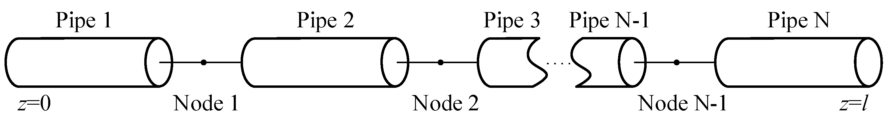
For the cascaded pipe, the overall transfer matrix can be expressed by a systematic multiplication of the field and point transfer matrices:

$${\mathbf{U}}_{\mathrm{a}\mathrm{l}\mathrm{l}}(s)={\mathbf{U}}_N(L_N,s)\cdots {\mathbf{U}}_i(L_i,s)\cdots {\mathbf{U}}_1(L_1,s)$$

(38)

where ${\mathbf{U}}_i$ is the transfer matrix of each pipe unit, and $L_i$ is the corresponding length.

Then, the boundary equation of the initial end of the cascaded pipe can be obtained from Equations (35) and (36):

$$\tilde{\mathsf{\Phi }}(0,s)={\mathbf{D}}^{*-1}\left(s\right)\mathbf{Q}\left(s\right)$$

(39)

where

$${\mathbf{D}}^{*}\left(s\right)=\left(\begin{array}{c}{\mathbf{D}}_0\left(s\right)\\ {\mathbf{D}}_L\left(s\right){\mathbf{U}}_{\mathrm{a}\mathrm{l}\mathrm{l}}(s)\end{array}\right),\mathbf{Q}\left(s\right)=\left(\begin{array}{c}{\mathbf{Q}}_0\left(s\right)\\ {\mathbf{Q}}_L\left(s\right)\end{array}\right)$$

(40)

It is easy to obtain $\tilde{\mathsf{\Phi }}(0,s)$ and ${\mathbf{U}}_{\mathrm{a}\mathrm{l}\mathrm{l}}(s)$ from Equations (38) and (39); hence, the variables $\tilde{\mathsf{\Phi }}(z,s)$ of any pipe sections mounted in the cascaded pipe system could be calculated.

4. Numerical Examples and Validation

4.1. Numerical Methods

4.1.1. Aircraft Hydraulic Pipe Model

In this section, the numerical calculation principles and methods performed for an aircraft hydraulic pipe contain diverse constraints and are systematically presented, which include the description of the pipe model and analysis condition, computing procedure of pipe boundary conditions, external excitations, and middle constraints.

The pipe includes eight straight and four elbow sections. Figure 6 and

Table 1. Physical parameters of the pipe and fluid.

Name	Notation	Value	Name	Notation	Value
Pipe length	L1	534.261 mm	Bending angle	$\Phi$	1.649 rad
	L2	72.996 mm	Pipe density	${\rho }_p$	7760 kg/m3
	L31, L32	61.630 mm	Young’s modulus	E	190 GPa
	L33	123.260 mm	Poisson’s ratio	$\upsilon$	0.27
	L4	72.996 mm	Oil density	${\rho }_f$	872 kg/m3
	L51, L52	267.131 mm	Bulk modulus	Kf	1.95 GPa
Outer diameter	D	9.525 mm	Kinematic viscosity	v	19.7 mm2/s
Pipe wall thickness	e	0.889 mm	Transducer mass	ms	0.006 kg
Bending radius	R	38.100 mm	Hydraulic oil brand	10# aircraft hydraulic oil

show the actual structure and detail parameters of the pipe, respectively; it is assumed that the material properties of each pipe segment are uniform.

For the above cascaded pipe of verification example, the overall transfer matrix can be written as:

$${\mathbf{U}}_{\mathrm{a}\mathrm{l}\mathrm{l}}={\mathbf{U}}_{L_{52}}{\mathbf{N}}_{A_2}{\mathbf{U}}_{L_{51}}{\mathbf{U}}_R{\mathbf{U}}_{L_4}{\mathbf{U}}_R{\mathbf{U}}_{L_{33}}{N}_P{\mathbf{U}}_{L_{32}}{N}_{A_1}{\mathbf{U}}_{L_{31}}{\mathbf{U}}_R{\mathbf{U}}_{L_2}{\mathbf{U}}_R{\mathbf{U}}_{L_1}$$

(41)

where $\mathbf{U}$ represents the field transfer matrix of each pipe section; ${\mathbf{N}}_A$ and ${\mathbf{N}}_P$ represent the point transfer matrix, considering the extra mass of the accelerometer and extra mass and stiffness of the elastic clamp, respectively.

The purpose-built verification system for aircraft hydraulic pipes containing diverse constraints is presented, as shown in Figure 7 (detailed description see Section 4.2). Four different working conditions and cases are designed to investigate the vibration response of aircraft hydraulic pipes in a wide range of fluid pressures and Reynolds numbers. According to the pipe diameter and critical Reynolds number (2320) of the smooth cylindrical pipe [1], the critical flow velocity is $V_1=4.80\mathrm{m}/\mathrm{s}$; detailed calculation parameters for four cases are shown in

Table 2. Detailed calculation parameters for four cases.

Cases	Flow Velocity (m/s)	Fluid Pressure (MPa)	Reynolds Number	Fluid State
1	2	5	967.01	Laminar
2	8	5	3868.02	Turbulence
3	2	10	967.01	Laminar
4	8	10	3868.02	Turbulence

, when setting the fluid pressures as 5 and 10 MPa, respectively.

4.1.2. Flow Pulsation Excitation

From Figure 7, it appears that the excitation at the left end of the pipe is fluid pulsation, and the flow fluctuation of hydraulic axial piston pump has been relatively maturely studied [1]. The rotational speed of the pump is set to 2000 r/min; when setting the pump flow as 6.82 and 27.3 L/min, the flow velocities are 2 and 8 m/s, respectively. Figure 8a and Figure 9a show that the flow pulsation of the hydraulic pipe can be obtained, and their spectra were further obtained in the frequency domain using the FFT method, as shown in Figure 8b and Figure 9b.

As shown in Figure 8 and Figure 9, the time domain curves of the flow pulsation change periodically with time; from the spectrum diagram, it can be seen that there are efficiency spikes at the fundamental frequency and its multiple frequencies, which means that the periodic function of the flow pulsation can be superimposed with a series simple harmonic pulsations. The first four natural frequencies, as well as the corresponding amplitudes, of the flow pulsation are compared in

Table 3. Spectrum characteristics of flow pulsation.

Flow Velocity (m/s)	f1 (Hz)	q1 (L/min)	f2 (Hz)	q2 (L/min)	f3 (Hz)	q3 (L/min)	f4 (Hz)	q4 (L/min)
2	227.8	0.033	484.1	0.006	711.9	0.004	939.7	0.003
8	227.8	0.132	484.1	0.024	711.9	0.017	939.7	0.011

.

The fluid excitation of the pipe can be set by flow velocity $V_e$ in the excitation matrix $\mathbf{Q}$; the specific method is: superimposing the sine function expressions, corresponding to the first four order frequencies after Laplace transform, which can be written as:

$$V_e(s)=V_{A1}{\omega }_1/(s^2+{\omega }_1{}^2)+V_{A2}{\omega }_2/(s^2+{\omega }_2{}^2)+V_{A3}{\omega }_3/(s^2+{\omega }_3{}^2)+V_{A4}{\omega }_4/(s^2+{\omega }_4{}^2)$$

(42)

where $\omega =2\pi f$ and $V=Q/A_f$; then, the angular frequency and amplitude of flow velocity spectrum characteristics are obtained, as shown in

Table 4. Spectrum characteristics of flow velocity.

Flow Velocity (m/s)	${\mathit{\omega }}_1$	VA1 (m/s)	${\mathit{\omega }}_2$	VA1 (m/s)	${\mathit{\omega }}_3$	VA1 (m/s)	${\mathit{\omega }}_4$	VA1 (m/s)
2	1430.584	0.008	3040.148	0.002	4470.732	0.001	5901.316	0.001
8	1430.584	0.034	3040.148	0.006	4470.732	0.004	5901.316	0.002

.

The throttle valve with a fixed opening is arranged at the right end of the pipe, where it has no external excitation. As boundary equations (Equation (21)), the excitation matrices used for numerical calculation can be expressed as:

$$\{\begin{array}{l}{\mathbf{Q}}_0(s)={\left[\begin{array}{ccccccc}{V}_e(s)& 0& 0& 0& 0& 0& 0\end{array}\right]}^{\mathrm{T}}\\ {\mathbf{Q}}_L(s)={\left[\begin{array}{lllllll}0\hfill & 0\hfill & 0\hfill & 0\hfill & 0\hfill & 0\hfill & 0\hfill \end{array}\right]}^{\mathrm{T}}\end{array}$$

(43)

4.1.3. Boundary Conditions

The boundary constraints at both ends of the pipeline are fixed supports, setting a large value (e¹²) as the stiffness coefficient to achieve the purpose of fixed supports. The velocity inlet at the left end of the pipe has been discussed above, and the pressure outlet can be represented by the linearity of the throttle valve, which is mounted at the right end of the pipe. The relationship between flow and differential pressure at both ends of the throttle valve is [1]:

$$P=k_q(V-{\dot{\omega }}_z)$$

(44)

where $k_q$ is throttle coefficient.

Then, calculate the throttle coefficients of four cases (Table 2), as shown in

Table 5. Throttle coefficient of the throttle valve in four cases.

Cases	1	2	3	4
kq	2.5 × 106	6.25 × 105	5 × 106	1.25 × 106

.

According to Equations (22) and (23), the boundary constraint matrices at the two pipe ends would be:

$${\mathbf{D}}_0(s)=\left[\begin{array}{cccccccccccccc}1& 0& -1& 0& 0& 0& 0& 0& 0& 0& 0& 0& 0& 0\\ 0& -A_f& -K_{z(0)}& 1& 0& 0& 0& 0& 0& 0& 0& 0& 0& 0\\ 0& 0& 0& 0& 1& -T_{y(0)}& 0& 0& 0& 0& 0& 0& 0& 0\\ 0& 0& 0& 0& 0& 0& -K_{x(0)}& 1& 0& 0& 0& 0& 0& 0\\ 0& 0& 0& 0& 0& 0& 0& 0& 1& -T_{x(0)}& 0& 0& 0& 0\\ 0& 0& 0& 0& 0& 0& 0& 0& 0& 0& -K_{y(0)}& 1& 0& 0\\ 0& 0& 0& 0& 0& 0& 0& 0& 0& 0& 0& 0& -T_{z(0)}& 1\end{array}\right]$$

(45)

$${\mathbf{D}}_L(s)=\left[\begin{array}{cccccccccccccc}-k_q& 1& k_q& 0& 0& 0& 0& 0& 0& 0& 0& 0& 0& 0\\ 0& -A_f& m_{L}s& 1& 0& 0& 0& 0& 0& 0& 0& 0& 0& 0\\ 0& 0& 0& 0& 1& 0& 0& 0& 0& 0& 0& 0& 0& 0\\ 0& 0& 0& 0& 0& 0& m_{L}s& 1& 0& 0& 0& 0& 0& 0\\ 0& 0& 0& 0& 0& 0& 0& 0& 1& 0& 0& 0& 0& 0\\ 0& 0& 0& 0& 0& 0& 0& 0& 0& 0& m_{L}s& 1& 0& 0\\ 0& 0& 0& 0& 0& 0& 0& 0& 0& 0& 0& 0& 0& 1\end{array}\right]$$

(46)

4.1.4. Middle Constraint

Section 2.3 discusses the middle constraint model and points out that the finite element analysis of the three-dimensional support model is usually conducted to obtain the parameters for one-dimensional calculation. A P-type clamp (HB3-25LB10B) containing a metal band and rubber cushion is used for verification; the detailed finite element modeling method and equivalent stiffness parameter calculation process for the clamp have been presented in [1], and the following six degrees of freedom equivalent stiffness parameters of the P-type clamp (

Table 6. Stiffness parameters of the P-type clamp [1].

Translational Stiffness (N/m)			Rotational Stiffness (N∙m/rad)
kx	ky	kz	tx	ty	tz
8.74 × 106	5.84 × 105	7.29 × 106	1830	239	1890

) are introduced to represent the stiffness impedance coefficient in the middle constraint matrix.

4.2. Experimental Methods

The schematic drawing and detailed layout of the experimental system are shown in Figure 10, including four major components: the hydraulic pump station unit, test pipe and its installation components, NI measurement system and data acquisition devices, and detailed specification of the equipment can be found in the appendix summary of [1]. The hydraulic pump station unit (maximum pressure can approach 35 MPa, with displacement up to 92 L/min) incorporates a motor-driven, seven-piston axial piston pump. The system flow can be altered by the swash angle of the hydraulic pump, and the fluid pressure is controlled by adjusting the opening of the electro-hydraulic proportional throttle valve. Both ends of the test pipe are connected with a rubber hose and mounted on the test bench. An elastic clamp is placed in the middle of the pipe and installed on the pipe bracket.

The fluid signals were constantly monitored via high-resolution flow and pressure sensors, arranged at the left and right ends of the pipe, respectively. The vibration signals of the pipe were collected with two lightweight acceleration sensors, which were mounted at measuring points A and B. The output voltage signals of the sensors were sent to the dynamic analyzer, in which the A/D convertor was mounted; the converter module connected via a USB port to a computer with the LabVIEW software, which performed the real-time data acquisition and sent control signals; then, the signals received in the dynamic tests were converted into the flow rate, fluid pressure, and vibration velocity.

4.3. Results and Discussions

4.3.1. Dynamic Response Characteristics of Fluid

Numerical calculations and experimental verifications of the dynamic response characteristics of fluid under four cases and configurations were conducted by setting the rotational speed of the pump to 2000 r/min and pump flow to 6.82 and 27.3 L/min, respectively, as well as adjusting the electro-hydraulic proportional throttle valve to set the system pressure to 5 and 10 MPa, respectively. The flow rate spectrum curves of the pipe inlet and fluid pressure spectrum curves of the pipe outlet were obtained, as shown in Figure 11 and Figure 12. Further, the comparison results of fluid pulsation harmonic frequencies are shown in

Table 7. Natural frequencies of the flow velocity of pipe inlet.

Cases	Item	First (Hz)	Second (Hz)	Third (Hz)	Fourth (Hz)
1,2,3,4	TMM method	228	484	712	940
1,3	Experiment results	225.97	484.97	714.74	938.52
	error (%)	0.89%	0.20%	0.38%	0.16%
2,4	Experiment results	225.68	485.48	714.82	938.10
	error (%)	1.02%	0.31%	0.40%	0.20%

and

Table 8. Natural frequencies of the fluid pressure of pipe outlet.

Cases	Item	First (Hz)	Second (Hz)	Third (Hz)	Fourth (Hz)
1,2,3,4	TMM method	228	484	712	940
1,3	Experiment results	227.80	481.65	709.40	926.94
	error (%)	0.09%	0.49%	0.37%	1.39%
2,4	Experiment results	228.15	484.55	712.12	930.47
	error (%)	0.07%	0.11%	0.02%	1.01%

.

As shown in Figure 11 and Figure 12, the flow velocity and pressure pulsation curves ranging from 0~1000 Hz all contain four harmonic frequencies (228, 484, 712, and 940 Hz), corresponding to the fluctuation harmonic frequencies of the axial piston pump, which shows the characteristics of the wide frequency domain and multi-harmonic frequency. Otherwise, the harmonic amplitude of fluid pulsation in the wide frequency domain shows an increasing trend, with increasing flow velocity and fluid pressure. It gradually decreases with the increasing harmonic order, and the change in the fundamental frequency response amplitude fluctuation is the most obvious. In addition, it can be seen that the variation law of the pipe outlet pressure spectrum curve is highly consistent with that of the inlet velocity spectrum curve, indicating that the flow pulsation is the main reason for stimulating the pressure pulsation, and the pulsation frequencies of both are the same.

Table 7 and Table 8 provide the comparison results of the fluid pulsation harmonic frequencies. From the results obtained in various cases, the maximum deviation of the numerical and experimental results was 1.39%. The amplitudes of both were different, and the numerical results were slightly larger than the experimental results. The principal reason may be that the absorption of fluid fluctuation was caused by the accumulator and filter assembled in the experimental system; however, these hydraulic components do not model comprehensively in numerical calculations. Nevertheless, the accuracy of the presented method is sufficient and applicable.

4.3.2. Dynamic Response Characteristics of Pipe

Numerical calculations and experimental verifications of the dynamic response characteristics of aircraft hydraulic pipe under four cases were conducted. Set the rotational speed of the pump to 2000 r/min and adjust the system flow and pressure, respectively, to match the four configurations in Table 2. The vibration velocity spectrum curves of pipe points A and B are shown in Figure 13, Figure 14, Figure 15 and Figure 16, where (a) represents the axial velocity of point A, (b) represents the radial velocity of point A, (c) represents the axial velocity of point B, and (d) represents the radial velocity of point B. Further, the comparison results of the pipe vibration response harmonic frequencies are listed in

Table 9. Resonant frequencies of pipe (case 1).

Order	Item	First (Hz)	Second (Hz)	Third (Hz)	Fourth (Hz)
	TMM method	228	484	712	940
(a)	experiment results	225.36	496.96	699.72	945.14
	error (%)	1.16%	2.68%	1.73%	0.55%
(b)	experiment results	226.43	486.86	696.08	947.98
	error (%)	0.69%	0.59%	2.24%	0.85%
(c)	experiment results	227.98	497.35	711.54	946.17
	error (%)	0.01%	2.76%	0.06%	0.66%
(d)	experiment results	227.14	484.19	711.05	957.23
	error (%)	0.38%	0.04%	0.13%	1.83%

,

Table 10. Resonant frequencies of pipe (case 2).

Order	Item	First (Hz)	Second (Hz)	Third (Hz)	Fourth (Hz)
	TMM method	228	484	712	940
(a)	Experiment results	225.08	497.84	696.29	938.25
	error (%)	1.28%	2.86%	2.21%	0.19%
(b)	Experiment results	224.82	489.51	699.60	948.20
	error (%)	1.40%	1.14%	1.74%	0.87%
(c)	Experiment results	226.99	498.32	703.13	941.67
	error (%)	0.44%	2.96%	1.25%	0.18%
(d)	Experiment results	222.28	481.22	703.01	956.00
	error (%)	2.51%	0.57%	1.26%	1.70%

,

Table 11. Resonant frequencies of pipe (case 3).

Order	Item	First (Hz)	Second (Hz)	Third (Hz)	Fourth (Hz)
	TMM method	228	484	712	940
(a)	Experiment results	222.06	496.98	699.18	937.25
	error (%)	2.60%	2.68%	1.80%	0.29%
(b)	Experiment results	226.09	485.07	697.24	957.71
	error (%)	0.84%	0.22%	2.07%	1.88%
(c)	Experiment results	228.52	493.49	710.63	955.68
	error (%)	0.23%	1.96%	0.19%	1.67%
(d)	Experiment results	223.59	482.09	698.24	948.25
	error (%)	1.93%	0.39%	1.93%	0.88%

and

Table 12. Resonant frequencies of pipe (case 4).

Order	Item	First (Hz)	Second (Hz)	Third (Hz)	Fourth (Hz)
	TMM method	228	484	712	940
(a)	Experiment results	224.19	502.87	699.27	968.98
	error (%)	1.67%	3.90%	1.79%	3.08%
(b)	Experiment results	220.72	484.23	713.45	956.63
	error (%)	3.19%	0.05%	0.20%	1.77%
(c)	Experiment results	229.63	488.91	711.10	953.61
	error (%)	0.72%	1.02%	0.13%	1.45%
(d)	Experiment results	228.03	479.45	710.04	949.04
	error (%)	0.01%	0.94%	0.28%	0.96%

.

Figure 13, Figure 14, Figure 15 and Figure 16 show that fluid pulsation leads to the large-amplitude forced vibration of the pipe; they show the vibration characteristics of multi-harmonic points in a wide frequency domain. Four obvious harmonic frequencies (228, 484, 712, and 940 Hz) with significant resonance peaks appear, ranging from 0~1000 Hz. The harmonic frequencies of pipe vibrations were consistent with the fourth-order harmonic frequencies of the fluid pulsation, indicating that, when the fluid harmonic frequencies and modal frequencies of the pipe come closer, a fluid–structure interaction resonance is caused.

A key point here is that, if the pipe length is not divided properly in the calculation process, there will be problems of overflow and calculation result instability in the frequency ranges after 700 Hz (a calculation example is shown in Figure 17). Although it does not affect the identification of resonant frequencies, the waveform of the response curves will change, and there will be other error frequencies.

This phenomenon will be more evident when the pipe is long or the calculation frequency range is wide. In order to avoid this pathological problem, the maximum length of a single pipe unit “z_max” should meet the following condition when using the transfer matrix method for calculation:

$$z_{\max }^2\le \frac{171}{c_p}\sqrt{\frac{E{I}_p}{M}}{\lambda }_{\min }$$

(47)

where ${\lambda }_{\min }$ is the wavelength of the bending wave of the smallest pipe wall in all pipe units.

When comparing the vibration response of the pipe under four cases, it was found that the amplitude of the radial vibration response is larger than that of axial vibration, overall, and the harmonic frequencies appeared obviously, indicating that the flow-induced vibration of the pipe is mainly large radial vibration, without considering other excitation sources. Interestingly, the vibration of point A in the high-frequency band mainly appears as axial vibration; that is because the position of point A is close to the elastic clamp, while the axial translational stiffness of the clamp is smaller than that of the radial translational stiffness (Table 6). That is, the axial restraint of the clamp on the pipe is relatively weak, which will make the axial vibration more obvious in the high-frequency band, indicating that the reasonable arrangement of the clamps in pipe systems can effectively reduce the transverse vibration of the pipe.

Moreover, the maximum harmonic response amplitude is the first-order harmonic frequency, and the pipe vibration velocity amplitude in the wide frequency domain shows a decreasing trend with the increasing harmonic order, indicating that the energy of the pipe vibration is mainly concentrated in the first few resonant frequencies. Therefore, increasing the pipe system’s fundamental frequencies is significant at the initial design phase and can help avoid low-order vibration frequencies in the pipe and prevent resonances.

The amplitude of pipe vibration response shows an increasing trend with the increasing flow rate, and the resonance frequencies do not change. The amplitude of pipe vibration response changes little, and the resonance frequencies also have no obvious change when there are variations in system pressure, indicating that the flow rate mainly affects the amplitude of pipe vibration; however, that does not change the vibration frequencies. Pressure has little effect on the vibration amplitude and frequencies. Therefore, inhibiting flow rate pulsation is a very effective method for reducing fluid–structure interaction resonance in pipe systems.

Table 9, Table 10, Table 11 and Table 12 provide the comparison results of the pipe vibration response harmonic frequencies in various cases. The numerical predictions display a satisfied consistence with experimental observations, and the maximum deviation is 3.90%, which may be comprehensively caused by errors in theoretical modeling and numerical solution from analytical approximations, pipe manufacturing errors and mounting deviations, random noises in test data, etc.

The observation results fully confirm that the presented theoretical model and experimental method can effectively deal with the fluid–structure interaction dynamics of aircraft hydraulic pipe with complex constraints in the frequency domain.

5. Conclusions

This paper studies the fluid–structure interaction dynamics of aircraft hydraulic pipes with complex constraints and boundary conditions, both numerically and experimentally, in the frequency domain. A partial differential fourteen-equation model accounts for the effects of pipe wall thickness, and high-speed, high-pressure fluid was applied to describe the nonlinear FSI dynamics of aircraft hydraulic pipe. The flow pulsation excitation model, fluid boundary conditions containing the velocity inlet and pressure outlet, and one-dimensional support constraint model considering the equivalent stiffness parameters were used to denote the complex constraints. These resulting equations were solved by the Laplace transform transfer matrix method (LTTMM) in the frequency domain. According to the numerical and experimental results, displayed in the form of the dynamic response characteristics of flow velocity, fluid pressure, and pipe vibration velocity, some important conclusions and interesting features are described as follows.

The developed FSI theoretical model and improved Laplace transform transfer matrix method (LTTMM) realized, from one analysis case to another, a simple modification of the matrix model parameters of the fluid and pipe structure, such as fluid excitations, boundary conditions, and support constraints. The method involves a few unified matrix models and does not require any modification to the solving course to obtain accurate results, which is especially suitable for the FSI dynamics analysis of aircraft hydraulic pipe with complex constraints in the broad frequency range.

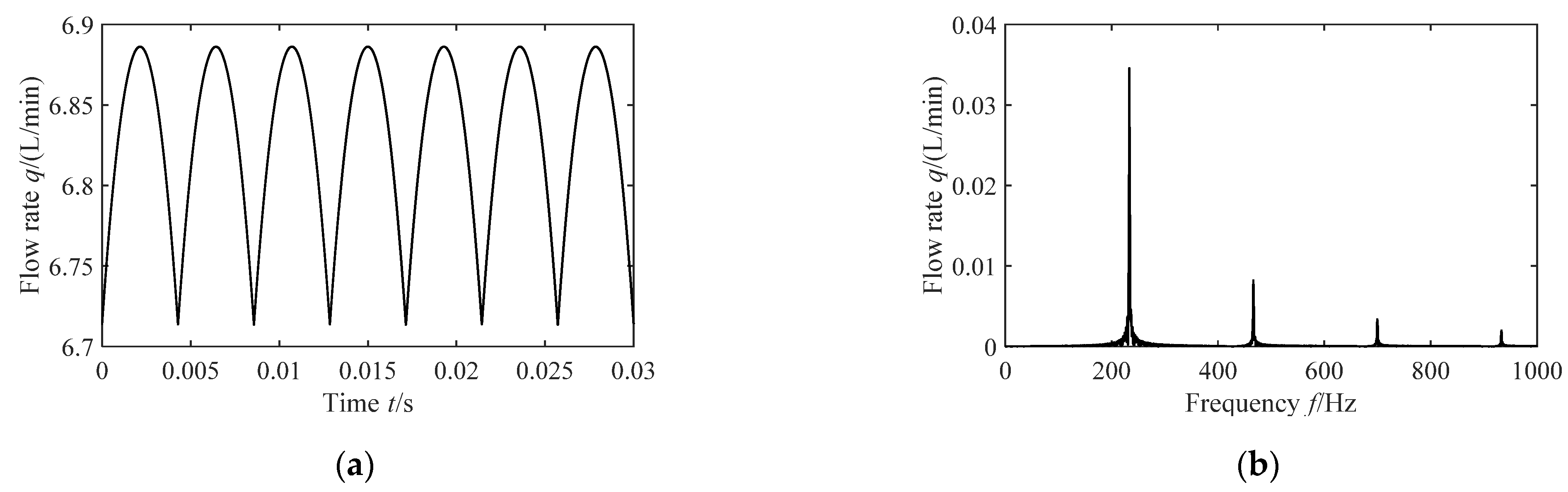
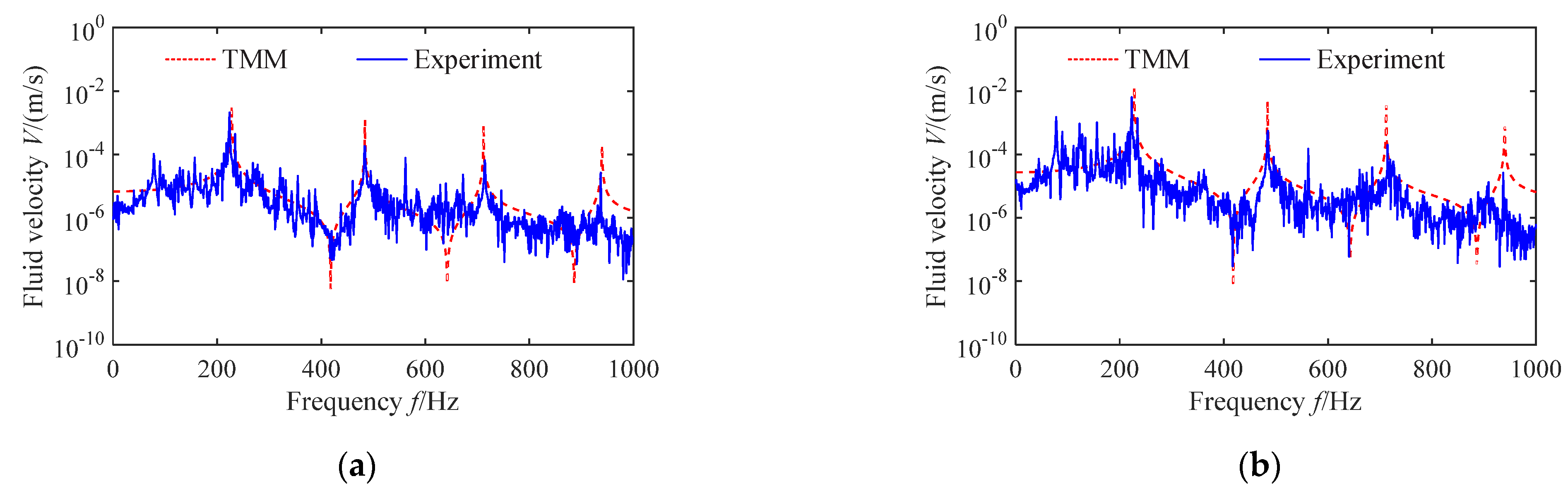
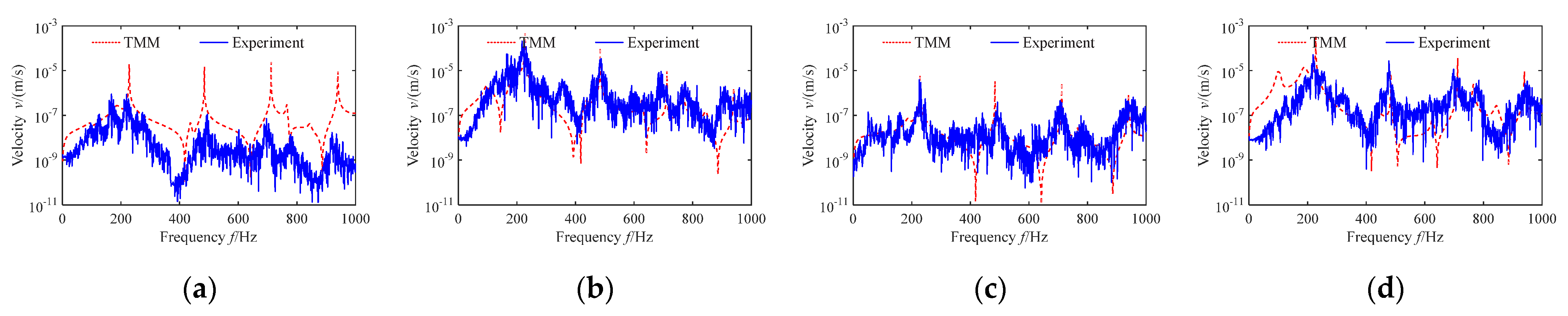
The harmonic amplitude of fluid pulsation in pipe systems showed an increasing trend, with increasing flow velocity and fluid pressure, and it gradually decreased with the increasing harmonic order. The change in the fundamental frequency response amplitude fluctuating was the most obvious, and flow pulsation was the main reason for stimulating the pressure pulsation. Flow-induced forced vibration of the pipe showed the characteristics of large-amplitude radial vibration and multi-harmonic points, without considering other excitation sources. The harmonic frequencies of pipe vibration were consistent with the harmonic frequencies of fluid pulsation. The maximum vibration velocity amplitude of the pipe was the first-order harmonic frequency, and the vibration velocity amplitude showed a decreasing trend with increasing harmonic order. The flow rate mainly affects the amplitude of pipe vibration, but that does not change the vibration frequencies, while the pressure has little effect on vibration amplitude and frequencies.

Furthermore, from the view of vibration control, a reasonable arrangement of the clamp in pipe systems can effectively reduce the transverse vibration; thus, increasing the fundamental frequencies of the pipe can avoid low-order high energy vibration in pipe systems, and inhibiting flow rate pulsation is a very effective method for reducing FSI resonance in pipe systems.

References

1. Gao, H.; Guo, C.; Quan, L. Fluid-Structure Interaction Analysis of Aircraft Hydraulic Pipe with Complex Constraints Based on Discrete Time Transfer Matrix Method. Appl. Sci. 2021, 11, 11918. [Google Scholar] [CrossRef]
2. Gao, P.; Yu, T.; Zhang, Y.; Wang, J.; Zhai, J. Vibration analysis and control technologies of hydraulic pipeline system in aircraft: A review. Chin. J. Aeronaut. 2021, 34, 83–114. [Google Scholar] [CrossRef]
3. Yang, Y.; Zhang, Y. Random vibration response of three-dimensional multi-span hydraulic pipeline system with multipoint base excitations. Thin Wall Struct. 2021, 166, 108124. [Google Scholar] [CrossRef]
4. Quan, L.; Che, S.; Guo, C.; Gao, H.; Guo, M. Axial Vibration Characteristics of Fluid-Structure Interaction of an Aircraft Hydraulic Pipe Based on Modified Friction Coupling Model. Appl. Sci. 2020, 10, 3548. [Google Scholar] [CrossRef]
5. Guo, X.; Ma, H.; Zhang, X.; Ye, Z.; Han, Q. Uncertain Frequency Responses of Clamp-Pipeline Systems Using an Interval-Based Method. IEEE Access 2020, 8, 29370–29384. [Google Scholar] [CrossRef]
6. Zhang, Y.; Liu, X.; Rong, W.; Gao, P.; Yu, T.; Han, H.; Xu, L. Vibration and Damping Analysis of Pipeline System Based on Partially Piezoelectric Active Constrained Layer Damping Treatment. Materials 2021, 14, 1209. [Google Scholar] [CrossRef]
7. Song, X.; Cao, T.; Gao, P.; Han, Q. Vibration and damping analysis of cylindrical shell treated with viscoelastic damping materials under elastic boundary conditions via a unified Rayleigh-Ritz method. Int. J. Mech. Sci. 2020, 165, 105158. [Google Scholar] [CrossRef]
8. Liu, X.; Sun, W.; Gao, Z. Optimization of Hoop Layouts for Reducing Vibration Amplitude of Pipeline System Using the Semi-Analytical Model and Genetic Algorithm. IEEE Access 2020, 8, 224394–224408. [Google Scholar] [CrossRef]
9. Gao, P.; Li, J.; Zhai, J.; Tao, Y.; Han, Q. A Novel Optimization Layout Method for Clamps in a Pipeline System. Appl. Sci. 2020, 10, 390. [Google Scholar] [CrossRef]
10. Zhang, Q.; Kong, X.; Huang, Z.; Yu, B.; Meng, G. Fluid-Structure-Interaction Analysis of an Aero Hydraulic Pipe Considering Friction Coupling. IEEE Access 2019, 7, 26665–26677. [Google Scholar] [CrossRef]
11. Zhai, J.; Li, J.; Wei, D.; Gao, P.; Yan, Y.; Han, Q. Vibration Control of an Aero Pipeline System with Active Constraint Layer Damping Treatment. Appl. Sci. 2019, 9, 2094. [Google Scholar] [CrossRef]
12. Yan, Y.; Zhai, J.; Gao, P.; Han, Q. A multi-scale finite element contact model for seal and assembly of twin ferrule pipeline fittings. Tribol. Int. 2018, 125, 100–109. [Google Scholar] [CrossRef]
13. Skalak, R. An extension of the theory of water hammer. Trans. ASME 1956, 78, 105–116. [Google Scholar] [CrossRef]
14. Wiggert, D.C.; Otwell, R.S.; Hatfield, F.J. The Effect of Elbow Restraint on Pressure Transients. J. Fluids Eng. 1985, 107, 402–406. [Google Scholar] [CrossRef]
15. Tijsseling, A.S. Water hammer with fluid–structure interaction in thick-walled pipes. Comput. Struct. 2007, 85, 844–851. [Google Scholar] [CrossRef]
16. Li, Q.S.; Yang, K.; Zhang, L.; Zhang, N. Frequency domain analysis of fluid–structure interaction in liquid-filled pipe systems by transfer matrix method. Int. J. Mech. Sci. 2002, 44, 2067–2087. [Google Scholar] [CrossRef]
17. Walker, J.S.; Phillips, J.W. Pulse propagation in fluid-filled tubes. J. Appl. Mech. Trans. ASME 1977, 77, 31–35. [Google Scholar] [CrossRef]
18. Davidson, L.C.; Smith, J.E. Liquid-structure coupling in curved pipes. Shock Vib. Bull. 1969, 40, 197–207. [Google Scholar]
19. Gale, J.; Tiselj, I. Eight equation model for arbitrary shaped pipe conveying fluid. In Proceedings of the International Conference Nuclear Energy for New Europe, Portoroz, Slovenia, 18–21 September 2006; pp. 610–616. [Google Scholar]
20. Wilkinson, D. Acoustic and mechanical vibrations in liquid-filled pipework systems. In Vibration in Nuclear Plant, Proceedings of International Conference, Keswick, UK, 12–14 May 1978; British Nuclear Energy Society: London, UK, 1979; pp. 863–878. [Google Scholar]
21. Tentarelli, S.C. Propagation of Noise and Vibration in Complex Hydraulic Tubing Systems. Ph.D. Thesis, Lehigh University, Bethlehem, PA, USA, 1990. [Google Scholar]
22. Wiggert, D.C.; Tijsseling, A.S. Fluid Transients and fluid-structure interaction in flexible liquid-filled piping. Appl. Mech. Rev. 2001, 54, 455–481. [Google Scholar] [CrossRef]
23. Liu, G.; Li, S.; Li, Y.; Chen, H. Vibration analysis of pipelines with arbitrary branches by absorbing transfer matrix method. J. Sound Vib. 2013, 332, 6519–6536. [Google Scholar] [CrossRef]
24. Xu, Y.; Johnston, D.N.; Jiao, Z.; Plummer, A.R. Frequency modelling and solution of fluid-structure interaction in complex pipelines. J. Sound Vib. 2014, 333, 2800–2822. [Google Scholar] [CrossRef]
25. Quan, L.; Meng, G.; Shi, J.; Jiao, Z.; Guo, C. Friction coupling vibration characteristics analysis of aviation hydraulic pipelines considering multi factors. High Technol. Lett. 2018, 24, 180–188. [Google Scholar]
26. Tan, X.; Mao, X.; Ding, H.; Chen, L. Vibration around non-trivial equilibrium of a supercritical Timoshenko pipe conveying fluid. J. Sound Vib. 2018, 428, 104–118. [Google Scholar] [CrossRef]
27. Wiggert, D.C.; Sundquist, J.M. Fixed-Grid Characteristics for Pipeline Transients. J. Hydraul. Eng. 1977, 103, 1403–1416. [Google Scholar] [CrossRef]
28. Tijsseling, A.S. Fluid-Structure Interaction in Case of Waterhammer with Cavitation. Ph.D. Thesis, Delft University of Technology, Delft, The Netherlands, 1993. [Google Scholar]
29. Tijsseling, A.S. Exact solution of linear hyperbolic four-equation system in axial liquid-pipe vibration. J. Fluids Struct. 2003, 18, 179–196. [Google Scholar] [CrossRef]
30. Xu, Y.; Jiao, Z. Exact solution of axial liquid-pipe vibration with time-line interpolation. J. Fluids Struct. 2017, 70, 500–518. [Google Scholar] [CrossRef]
31. Sreejith, B.; Jayaraj, K.; Ganesan, N.; Padmanabhan, C.; Chellapandi, P.; Selvaraj, P. Finite element analysis of fluid-structure interaction in pipeline systems. Nucl. Eng. Des. 2004, 227, 313–322. [Google Scholar] [CrossRef]
32. Zhang, Y.L.; Gorman, D.G.; Reese, J.M. A finite element method for modelling the vibration of initially tensioned thin-walled orthotropic cylindrical tubes conveying fluid. J. Sound Vib. 2001, 245, 93–112. [Google Scholar] [CrossRef]
33. Ruoff, J.; Hodapp, M.; Kück, H. Finite element modelling of Coriolis mass flowmeters with arbitrary pipe geometry and unsteady flow conditions. Flow Meas. Instrum. 2014, 37, 119–126. [Google Scholar] [CrossRef]
34. Ahmadi, A.; Keramat, A. Investigation of fluid-structure interaction with various types of junction coupling. J. Fluids Struct. 2010, 26, 1123–1141. [Google Scholar] [CrossRef]
35. Achouyab, E.H.; Bahrar, B. Numerical modeling of phenomena of waterhammer using a model of fluid-structure interaction. Comptes Rendus Mécanique 2011, 339, 262–269. [Google Scholar] [CrossRef]
36. Li, S.; Liu, G.; Kong, W. Vibration analysis of pipes conveying fluid by transfer matrix method. Nucl. Eng. Des. 2014, 266, 78–88. [Google Scholar] [CrossRef]
37. Liu, G.; Li, Y. Vibration analysis of liquid-filled pipelines with elastic constraints. J. Sound Vib. 2011, 330, 3166–3181. [Google Scholar] [CrossRef]
38. Zhang, L.; Tijsseling, S.A.; Vardy, E.A. Fsi Analysis of Liquid-Filled Pipes. J. Sound Vib. 1999, 224, 69–99. [Google Scholar] [CrossRef]
39. Lesmez, M.W.; Wiggert, D.C.; Hatfield, F.J. Modal Analysis of Vibrations in Liquid-Filled Piping Systems. J. Fluids Eng. 1990, 112, 311–318. [Google Scholar] [CrossRef]
40. Li, S.J.; Karney, B.W.; Liu, G.M. FSI research in pipeline systems—A review of the literature. J. Fluids Struct. 2015, 57, 277–297. [Google Scholar] [CrossRef]
Figure 1. Schematic of the pipe section conveying fluid.
Processes 10 01161 g001
Figure 2. Local coordinate systems of boundary nodes. Reprinted with permission from Ref. [24]. Copyright © 2013 Elsevier Ltd. All rights reserved.
Processes 10 01161 g002
Figure 3. Local coordinate systems of middle node. Reprinted with permission from Ref. [24]. Copyright © 2013 Elsevier Ltd. All rights reserved.
Processes 10 01161 g003
Figure 4. Schematic of the cascaded pipe units and nodes. Reprinted with permission from Ref. [24]. Copyright © 2013 Elsevier Ltd. All rights reserved.
Processes 10 01161 g004
Figure 5. Transfer matrices of pipe. (a) Field transfer matrix. (b) Point transfer matrix. Reprinted with permission from Ref. [24]. Copyright © 2013 Elsevier Ltd. All rights reserved.
Processes 10 01161 g005
Figure 6. Analysis model of the aircraft hydraulic pipe.
Processes 10 01161 g006
Figure 7. Schematic of the verification system.
Processes 10 01161 g007
Figure 8. Flow pulsation excitation (flow velocity is 2 m/s). (a) Pulsation curve in time domain. (b) Pulsation curve in frequency domain.
Processes 10 01161 g008
Figure 9. Flow pulsation excitation (flow velocity is 8 m/s). (a) Pulsation curve in time domain. (b) Pulsation curve in frequency domain.
Processes 10 01161 g009
Figure 10. Experimental system and test stand layout.
Processes 10 01161 g010
Figure 11. Flow velocity of pipe inlet. (a) Cases 1 and 3. (b) Cases 2 and 4.
Processes 10 01161 g011
Figure 12. Fluid pressure of pipe outlet. (a) Cases 1 and 2. (b) Cases 3 and 4.
Processes 10 01161 g012
Figure 13. Velocity responses of pipe (case 1). (a) Axial velocity of point A. (b) Radial velocity of point A. (c) Axial velocity of point B. (d) Radial velocity of point B.
Processes 10 01161 g013
Figure 14. Velocity responses of pipe (case 2). (a) Axial velocity of point A. (b) Radial velocity of point A. (c) Axial velocity of point B. (d) Radial velocity of point B.
Processes 10 01161 g014
Figure 15. Velocity responses of pipe (case 3). (a) Axial velocity of point A. (b) Radial velocity of point A. (c) Axial velocity of point B. (d) Radial velocity of point B.
Processes 10 01161 g015
Figure 16. Velocity responses of pipe (case 4). (a) Axial velocity of point A. (b) Radial velocity of point A. (c) Axial velocity of point B. (d) Radial velocity of point B.
Processes 10 01161 g016
Figure 17. Calculation results overflow error example (case 1, point A).
Processes 10 01161 g017