Abstract
One of the consequences of the widespread automation of manufacturing operations has been the proliferation and availability of historical databases that can be exploited by analytical methods to improve process understanding. Data science tools such as dimension reduction and clustering are among many such approaches that can aid in the identification of unique process features and patterns that can be associated with faulty states. However, determining the number of such states still requires significant engineering knowledge and insight. In this study, a new unsupervised method is proposed that reveals the number of classes in a data set. The method utilizes a variety of dimension reduction techniques to create projections of a data set and performs multiple clustering operations on the lower-dimensional data as well as the original data. The relevant internal clustering metrics are incorporated into a multi-objective optimization problem to determine the solutions that simultaneously optimize all metrics. The cluster number that shows Pareto optimality based on the performance metrics is selected as the final one. The method is tested on three data sets with distinct features. The results demonstrate the ability of the proposed method to correctly identify the expected number of clusters.
1. Introduction
Constant monitoring of operational variables throughout the systems of manufacturing processes results in massively archived databases. As this historical record of operations is high-dimensional and complex, it presents a valuable opportunity to discover operational patterns and behaviors, and, as a result, to detect possible faults and anomalous behaviors. In most cases, an adequate analysis of anomalies is only possible after the event; therefore, carrying out a post mortem study of historical data becomes critical. As a result, many fault detection methods utilizing high-dimensional historical data have been developed throughout the years [1,2].
The historical data collected as such contains (or at least is expected to contain) information that can be exploited for modeling, prediction and anomaly detection/isolation in various industries. Depending on the size and the complexity of operations, such data can be low-dimensional or high-dimensional, where in the latter case the process of information extraction becomes more challenging. Hence, big data analysis has drawn more attention in the search for ways to facilitate knowledge discovery [3]. The approach presented in this study is generic and can be applied to historical data sets from a variety of industries and systems.
Two tools that are frequently used in information extraction from and the visualization of complex data sets are dimension reduction and clustering methods. Over the years, a variety of approaches have been developed for each of these tools, and one needs to be cognizant of the underlying science that makes them appropriate for some data sets and not necessarily others. Often, a certain amount of insight is required to select the best-performing method; however, this becomes problematic in many real-life cases. Hence, understanding the approach behind each technique can help in guiding the analyst towards the appropriate selection from the available methods. This lack of clarity has led to the use of these methods often in an unsupervised manner [4]. Dimension reduction (DR) techniques are one category of highly useful tools that can transform the original high-dimensional data set to a data set with lower (thus, more manageable) dimensions by preserving specific characteristics of the original data, with the goal of retaining the most important features and information. In [5], the authors have presented a comprehensive review of the most widely used DR techniques and offer a thoughtful analysis of their performance. The other aforementioned tool—clustering—serves the purpose of information extraction by finding particular groupings (or clusters) within the data (classification). These clusters of data points are identified based on the similar characteristics of their members, where each cluster would represent a physically meaningful class. The definition of similarity for clustering the points varies among different approaches. The review article presented by [6] discusses clustering analysis and a number of algorithms thoroughly. Separate studies of each of these tools have also been carried out in the context of practical applications, and they have been evaluated based on their success in class representation. They have proven to be beneficial in developing data-driven methods for process monitoring and fault detection/diagnosis as compiled by [7,8]. Furthermore, the performance of and the synergy between DR techniques and clustering methods have been studied considering various combinations and permutations, and a detailed analysis has been presented by [9]. However, the matter of obtaining optimal results (combinations) is a subject that requires further discussion, especially if these methods are used in cases without any prior knowledge about the data.
2. State-of-the-Art Techniques
The most common observation in performing clustering analysis on a data set is that the odds of obtaining satisfactory results are low, especially if there is not enough prior knowledge about the data set. This is an outcome of the parametric dependence of the clustering methods on data features. In addition, as in most real-life scenarios, since a priori information is not available, performance evaluation can only be conducted using internal metrics. Most of these validation metrics optimize parameters, which is also the objective of the clustering methods [10], so these metrics might not offer a true representation of the data under scrutiny. For example, the Silhouette coefficient is more compatible with k-means, and the Density-Based Clustering Validation (DBCV) index is more compatible with HDBSCAN (a detailed discussion of these metrics are presented later in Section 3.4). Therefore, evaluating internal validation criteria is a matter that has been examined through various studies to measure the ability of these metrics in representing the success of clustering results [11].
Multiple studies have been performed in the last few decades addressing the performance of internal validation criteria, each focusing on different information to report, such as the ability to identify the correct number of clusters, assessing the correct grouping of data points and selecting the best parameter settings for each algorithm [11]. One of the first studies was carried out by [12], and 108 small, artificial data sets were used to identify the correct number of clusters for hierarchical clustering. They reported that the Calinski–Harabasz (CH) index was the best-performing one. In a more recent study by [13], four validation criteria—Silhouette, Davies–Bouldin, CH, and DBCV Index—were used on 27 data sets to identify the highest scoring solution and the best parameters for each of the six clustering algorithms; k-means, DBSCAN, Ward, Expectation-Minimization (EM), mean-shift and spectral clustering. One of their results indicated that k-means is easily capable of achieving good Silhouette and CH scores, and DBSCAN works best with DB and DBCV indices.
When faced with multiple indices for assessing performance, a reasonable approach would be to consider an ensemble of these indices. Then, naturally, the matter of partial weights and metrics combinations arise. Another approach would then lie in exploring a framework in which more than one index is considered at a time to discover the patterns underlying the data, hence the best possible clustering solution. As a result, it seems appropriate to formulate the problem as a multi-objective optimization problem. Multi-objective optimization, or Pareto optimization, is an optimization problem that has, as the name suggests, more than one objective function to optimize. Pareto optimal or non-dominated solutions are the solutions in which none of the objective functions can be improved without degrading another one, thus producing the set of most acceptable solutions. Realistically, this also means that there exists no solution that has every objective simultaneously optimized (maximized or minimized). Therefore, in the end, a set of solutions are deemed equally acceptable and presented to the decision maker [14]. There are three major approaches to multi-objective optimization problems: (i) using a weighted sum to combine a set of objectives into a single objective, (ii) ordering the objectives based on their importance, or (iii) optimizing the multiple objectives simultaneously with a Pareto-based approach [15]. The latter provides a set of solutions from which the decision maker will select (or evaluate).
Multi-objective clustering (MOC) has been of growing interest in recent years, especially in the field of genetic algorithms [16]. Keeping in mind that, realistically, optimizing no single objective can completely capture the clusters present in a data set, MOC performs a search over the space of all parameters of the algorithm while simultaneously optimizing a number of validity indices. An algorithm named MOCK (Multi-Objective Clustering with automatic determination of the number of clusters), presented by [17], offers a multi-objective evolutionary algorithm to detect the correct number of clusters in a genetic encoding, and its objective functions are the overall deviation of partitioning (which is the overall summed distances between data points and their cluster centers) and connectivity (which measures the degree that neighboring data points have been placed in the same cluster). In another work performed by [18], the NSGA-II algorithm has been used on numeric image data sets to simultaneously optimize the Xie–Beni (XB) index (which is a ratio of global to local variation) and (which calculates the global cluster variance), and the results are compared to two other scenarios, each optimizing only one of these scores using other clustering methods. The final results are evaluated using another index that was not included before and suggest that the multi-objective clustering outperforms the other methods.
Considering the previous work and aforementioned advantages of MOC, this study considers a clustering strategy using Pareto optimization to simultaneously optimize a number of different metrics to reveal the behavior of the data. Hence, the clustering result will not depend on only one metric (and one type of cluster feature), but rather a more holistic view is taken into account to assign the memberships. In more detail, the clustering would be treated as an unsupervised step of data analysis, with none of the parameters selected. The clustering is performed multiple times while varying the parameters over their ranges, and multiple internal metrics are calculated for each run. A multi-objective optimization is then performed, with these metrics as objectives, to find the best solutions and the final number of present clusters. To obtain a better insight, the previous step is then combined with DR techniques to further assist the information extraction. Depending on how the mapping is carried out from high dimensions to low dimensions, different clusters can be created or lost. Therefore, considering representations of the data set at hand in various versions in lower dimensions would help in identifying the patterns/clusters that are preserved during the mapping, i.e., the most persistent features of the data. Finally, MOC is performed multiple times on different projections of the data to assess the results of the clustering step.
In comparison to previous studies focusing on multi-objective clustering, the novel features of the current study are (1) the consideration of a density-based validity metric as well as cohesion-based and separation-based indices simultaneously, as well as (2) the utilization of DR techniques and the application of multi-objective clustering in tandem to discover the most important features of a data set. As a tangible result of the methodology, the presented robust solution, which approaches the problem from different aspects, provides an unsupervised tool to determine the optimal number of clusters that can be used as an input to subsequent analyses contributing to the final solution. Hence, the expert knowledge requirement of such unsupervised analysis techniques can be significantly reduced, and the implementation can be automatized.
The roadmap of the article is as follows. In the next section, the problem formulation, overview of the methods and objective functions, as well as details of the data sets for the case studies and the steps of the proposed approach are presented. Results and discussion of the numerical experiments on the mentioned data sets are presented in Section 3, and Section 4 offers the conclusions.
3. Methodology
In this section, a brief overview of the methods utilized in this study is presented, starting with the general mathematical formulation of the problem, followed by the discussion of the methods of dimension reduction and clustering. Then, the performance metrics/indices, the multi-objective optimization problem and finally the data sets are introduced. The section concludes with the specific steps of the proposed method.
3.1. Problem Formulation
The schematic representation of the proposed methodology is depicted in Figure 1. We start formulating the problem at the top left corner of the figure by assuming an data matrix , where n denotes the number of samples and m is the number of variables. During the first step, the dimension reduction is performed (top in the middle in Figure 1), where the aim of dimension reduction is to map the matrix onto a matrix by preserving as much of the intrinsic structure of the data set as possible where the set of vectors is of a reduced dimension p ():
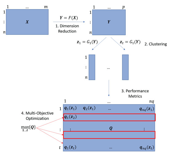
Figure 1.
The schematic representation of the proposed methodology with its four main steps: dimension reduction, t types of clustering, the characterization of the clustering solutions by metrics and the selection of the best solutions.
Again, the function G is defined based on the selected clustering method. Here, the outcome is an vector, where the elements correspond to the subsets with the number of clusters k. In addition, it is assumed that there exists a true set of labels defined by a vector , where the elements are of the subsets of true labels with the number of labels represented by .
Recognizing that clustering is an unsupervised machine learning technique, the determination of the true (distinguishable) number of clusters, , is often based on the expert knowledge of the application domain and in several cases may be required as an input to the clustering algorithm. The aim of the present article is to determine the optimal number of clusters, k, in an unsupervised manner. Therefore, during Step 2, with the application of t different clustering techniques, t different possible clustering solutions are created, resulting in a total of t vector s. Subsequently, in the third step, the resultant clustering solutions are evaluated based on different internal metrics, which are calculated with the help of functions. The results of these calculations are stored in a matrix . This is followed by the determination of the optimal solutions from the t solutions by multi-objective optimization, and further Pareto-front-based analysis reveals the optimal number of subsets (the proposed method is described in depth in Section 3.6). This optimization-based selection of results and determination of the optimal cluster number is depicted as Step 4 in Figure 1. As a result of this robust scoring method, applying multiple clustering solutions and multiple evaluation metrics, and hence approaching the problem from various aspects, the number of found clusters and the number of true (distinguishable) subsets in the data set are found to be equal, i.e., without the prior knowledge of the number of true (distinguishable) subsets, ). To demonstrate the performance of the proposed method, is compared to k in the end. The general formulation of the multi-objective optimization problem in Step 4 with objective functions is presented as
Or, in more explicit form,
Due to the often conflicting objective functions, the solution of a multi-objective optimization problem is typically not a single point but a group of points called the Pareto-optimal or non-dominated set of solutions. A non-dominated solution is defined as the solution that is strictly better than the rest of the solutions in at least one criterion and is no worse than the rest in all objectives. In other words, a non-dominated solution cannot improve in any of the objectives without degrading at least another one and is accordingly selected as a member of the final solution set. This set of non-dominated solutions is called Pareto-optimal [19].
In the present work, the goal is to analyze the Pareto optimal solutions of the t solutions. The form of the applied dimension reduction functions, F, are defined in Section 3.2, while the approaches for clustering—therefore, the form of the function G—are provided in Section 3.3. Finally, the objective functions, or in other words, the internal evaluation metrics (indices) of clustering performance, are provided in Section 3.4, as well as external metrics for a final assessment of the proposed approach.
3.2. Dimension Reduction (DR) Techniques
The main use of DR techniques is to remove redundant information (data) and represent meaningful features of the raw process data in fewer—often, two or three—dimensions (2D or 3D). Some benefits of applying DR techniques are reducing the computational complexity and avoiding the curse of dimensionality. While having a lower number of (transformed) variables facilitates data analysis, these techniques can also be used for visualization purposes in 2D or 3D. For the case at hand, all DR techniques have been used to transform the original m-dimensional data set into a two-dimensional manifold. A brief introduction to the DR techniques used in this study follows, with a focus on their definitive attributes, which classify them into three different categories of correlation-preserving, distance-preserving and neighborhood-preserving.
- Principal Component Analysis (PCA) Principal Component Analysis [20,21] is by far the most well-known dimension reduction technique with applications in diverse fields. Very briefly, PCA assumes that there exists a new set of variables called the principal components (PCs) that is smaller than the original number of variables, through which the original interrelated (correlated) data can be expressed. These new variables, which are linear combinations of the original variables, are uncorrelated and orthogonal, and this linear projection is constructed in such a way to preserve the maximum variation possible present in the original data. The number of selected principal components in the end determines the number of dimensions of the PC space. As can be gleaned from this description, this method is a correlation-preserving technique. PCA and all its derivatives are considered to belong to this category.
- Multidimensional Scaling (MDS)Multidimensional Scaling [20,22] is an example of the distance-preserving category. It is assumed that the relative distance between points in the original data is more informative than their correlation; therefore, the goal is to preserve that distance during the dimension reduction step. Given the proximity matrix (which is simply the table of Euclidean distances), a map displaying the relative positions of the data points is constructed and then used to find the points in the lower dimensions. Since this is performed based solely on the distance, any shift/rotation of the data will produce the same proximity matrix; therefore, there can be many solutions. Hence, a centering step is preformed to pin down one solution. A variation of MDS is the Metric MDS, which is for quantitative data, and its algorithm has a few differences such as the distance matrix and the loss function.An important matter regarding the inefficiency of linear techniques (such as PCA and MDS), which has been considered in the recent years, is the importance of the data structure rather than the Euclidean distance. Two points may be close to each other based on their Euclidean distance, but they may be far in the data manifold based on their geodesic distance. Therefore, it is advisable to also consider nonlinear manifold DR techniques to compare their results with linear methods.
- Isometric Mapping (ISOMAP)Another example of the distance-preserving category of DR techniques is ISOMAP [23], which is closely related to MDS. To address the inefficiency of Euclidean distance, this method preserves the geodesic distance of the data manifold by constructing a neighborhood graph using the nearest neighbors of each point and calculating the shortest path between pairs of data points through their closest neighbors. After that, by following the steps of MDS, a distance matrix is constructed to use for dimensionality transformation. This results in a nonlinear projection of the original manifold.
- t-Stochastic Neighborhood Embedding (t-SNE)The next category is the neighborhood-preserving techniques. t-Stochastic Neighborhood Embedding (t-SNE) [24] is an example of this category, which assumes that local neighborhoods are more important in revealing the inner structure of the data. This method attempts to preserve the local neighborhoods by creating a Gaussian probability distribution of each neighborhood and transferring them to the lower dimensions using a t-student distribution while minimizing a cost function. Because of the “heavy tails” probability of t-distribution, the relative distances become more extreme, thus highlighting the local neighborhoods more clearly. Since this algorithm works only with local neighborhoods, any global structure—or in other words, distance between clusters in the high dimensions (or higher dimensional features)—may be lost in the low-dimensional representation.
- Uniform Manifold Approximation and Projection (UMAP)Uniform Manifold Approximation and Projection (UMAP) [25] is a manifold-learning dimension reduction technique and is in the same category of neighborhood-preserving techniques, being similar to t-SNE. However, it has some differences in the way that the conditional probability calculations are carried out and how the cost function is formulated in trying to preserve the global structure as well by balancing the local–global structure preservation. In addition, it has a faster execution time compared to t-SNE.
3.3. Clustering Methods
Four different categories of clustering methods are utilized in this study: connectivity-based, centroid-based, distribution-based and density-based.
- Connectivity -based clusteringThe methods in this category consider the spatial (often Euclidean) distance between data points when assigning cluster membership. Closer data points are assumed to be in similar clusters as opposed to farther data points. The most well-known method in this category is agglomerative hierarchical clustering [26], which uses a number of possible closeness measures (linkages). This method uses a bottom-up merging strategy, starting by considering every data point as a single cluster and then merging the two closest clusters together, and repeating this process until the whole data set belongs to one cluster. The hierarchy of these combinations is represented by a dendrogram in the shape of a tree. After the process is completed, the user can choose where to cut the dendrogram, therefore defining the number of clusters.
- Centroid-based clusteringMethods in this category find centroids in order to partition the data into a specific number of clusters. This is performed by minimizing the distance of points from their closest centroid. The examples chosen for this category are k-means [27] and k-medoids [28]. The main difference between these two methods is their selection of the centroid. For k-means, the algorithm uses the number of clusters, k, as the input by the user and tries to separate the data into k groups of equal variance, while minimizing the sum of squares of distances for members of a cluster from the centroid of that cluster. The centroids are randomly chosen in the beginning and are updated through each iteration of the algorithm to be the mean of their cluster members. This randomness slightly affects the results in every run. While k-medoids is similar to k-means, it instead minimizes a sum of general pairwise dissimilarities, and the medoids (centroids) are determined from the points in the data set.
- Distribution-based clusteringThe main idea exploited in this third category is the assumption that members of a cluster most likely belong to the same distribution, in other words, points are assigned to clusters based on their probability of belonging to a distribution. A Gaussian mixture model (GMM) [29], for example, assumes that the data are constructed of multiple Gaussian distributions. This method uses the Expectation-Maximization algorithm to find the parameters of each Gaussian to finally determine the probabilities of each sample belonging to any Gaussian distribution.
- Density-based clusteringIn the fourth category, clusters are defined as areas of high density separated by areas of low density. Higher density is defined as smaller regions with higher numbers of samples, and based on this definition, all methods in this category are able to perform outlier detection. Density-Based Spatial Clustering of Applications with Noise (DBSCAN) [30] is one example that finds core samples as data points that have a minimum number of samples within a specified distance around them and therefore finds dense areas using that distance. Ordering Points To Identify the Clustering Structure (OPTICS) [31] is very similar to DBSCAN, with a major difference: OPTICS orders the points in a reachability graph to prioritize the memberships, which allows for variable density cluster identification in a single data set. Hierarchical density-based clustering (HDBSCAN) [32] is also similar to DBSCAN, but has a hierarchical approach. The clusters are searched for using a range of distances, but instead of the size of the region determining this separation cut, the cut is placed where the number of small clusters and outliers are reasonable; i.e., the formed clusters are more stable. The input parameter is the minimum cluster size to help the algorithm make the cut in the dendrogram.
3.4. Performance Evaluation Metrics
The performance assessment of clustering methods depends on an important piece of information about the data: whether the true assignments of data points (i.e., true labels) are known or not. Cases with known true labels are usually used for training and classification (supervised) purposes, and metrics are called external. There are a number of important metrics that are calculated using the true labels and clustering assignments. The metrics considered in this study are Adjusted Mutual Information (AMI) and V-measure. These indices provide a more accurate assessment of how the clustering was performed. For the purposes of this study, external metrics are only introduced and later utilized to demonstrate the performance of the approach and are not objective functions for the optimization process. Later in this section, internal metrics are introduced, such as the Silhouette coefficient, Davies–Bouldin index and DBCV index. These constitute the objective functions of the optimization to find the expected number of clusters and are the calculated metrics for each solution.
3.4.1. Adjusted Mutual Information (AMI)
Adjusted Mutual Information (AMI) [33] is the adjustment of the Mutual Information score to measure the agreement between true labels and assignments while accounting for chance and is an external metric. The mathematical description follows the steps below:
Consider two assignments of the vector , with clusters and with clusters. Selecting an object randomly from , the probability of the object falling into cluster is expressed as
where is the number of elements in cluster . The entropy S of a set represents the amount of uncertainty for a partition set:
The mutual information between the sets and is then expressed as
where is the probability that a sample point belongs to cluster in the assignment and to cluster in the assignment . The expected value of MI is calculated according to the following:
For easier notation, is the number of elements in and is the number of elements in . denotes the number of objects common to clusters and . The variables and are the partial sums of the contingency table of predicted and true (expected) labels: and . denotes . The final AMI score is calculated as
The AMI score is bounded between 0 and 1, where assuming that one of the assignments contains the true cluster labels, the higher values correspond to better performing clustering assignments.
3.4.2. V-Measure
Another external metric is calculated using two other performance metrics: homogeneity (h) and c ompleteness (c). The former is calculated based on whether each cluster only contains members of a single class, and the latter regards whether all members of a given class are assigned to the same cluster. Each is calculated as follows:
where and are the entropy values of sets and , while is the conditional entropy of the classes, given the cluster assignment:
where is the number of samples belonging to class and assigned to class . The harmonic mean of these scores is called the V-measure [34], bounded between 0 and 1, where higher values represent more accurate clustering assignments:
As most cases consider unsupervised approaches where the true labels of the data are not known, the performance assessment of the clustering assignments is carried out using the internal metrics, with the help of internal features of the found clusters. These features can be placed into two categories: cohesion measures and separation measures [10]. Cohesion can be interpreted as the tightness of the found clusters, and separation represents how “far” the clusters are from each other. Clusters are ideally defined as groups of points that have high cohesion and high separation. However, the tightness of each of the clusters and distance of pair of clusters measure the same metrics that the clustering methods optimize to detect clusters. Therefore, these evaluation metrics and most clustering methods validate each other’s results. As a result, the outcome may not be truly representative of the actual clusters and structure of the data.
3.4.3. Silhouette Coefficient
The most well-known internal metric is the Silhouette coefficient [35]. Similar to most of the internal validation metrics, this metric is the ratio of cohesion to separation, and maximization of the metric is favorable. For a data point l in cluster , the simplified formula is
where A is the mean distance between a sample and all other points in the same cluster :
and B is the smallest mean distance between a sample and all other points in the next nearest cluster :
For this metric to be maximized (it has an upper bound of 1 and a lower bound of −1), it is ideal for A to be much smaller than B. A high value indicates that the object is well matched to its own cluster and poorly matched to neighboring clusters. The Silhouette coefficient, , is calculated for all points, and the overall is the mean over all data points.
3.4.4. Davies–Bouldin (DB) Index
Another example of internal metrics is the Davies–Bouldin (DB) index [36], which compares the distance between clusters with the size of the clusters themselves. Two scores are calculated: T and M. T is the average distance between each point of cluster and the centroid of that cluster (cluster diameter).
where is the feature vector assigned to the cluster, is the centroid of the cluster, is the size of the cluster, and p is usually 2 to consider a Euclidean distance (2-norm). M is the distance between cluster centroids:
A value of is then calculated for each pair of clusters:
The DB Index is found using the maximum of values:
where k is the number of clusters.
Based on previous definitions, it would be ideal to have a high value of M and a low value of T, and therefore a low value of the DB index. The lower values would then indicate a model with better separation between clusters. The index has a minimum of zero.
In addition, there are some other examples such as the Dunn index [37] and Calisnki–Harabasz index [38] with similar structures. Clearly, a problem arises in cases that do not have convex clusters, including cases with elongated or arbitrary-shaped clusters, as these clusters will not achieve good scores regarding these metrics. Furthermore, most of these metrics do not account for any possible unclustered data points (outliers) that might have been found using some of the clustering methods. Hence, a need for an internal clustering evaluation metric with different features is evident.
3.4.5. Density-Based Clustering Validation (DBCV) Index
There have been some recent studies that have proposed new metrics that work with other features of the clusters, such as density, and thus could be more suitable to assess the performance of density-based clustering methods. The most well-developed metric is the Density-Based Clustering Validation (DBCV) index [39]. Similar to objectives of density-based clustering methods, this internal metric considers the relative density connections between pairs of objects. The all-points-core-distance, which is the inverse of the density of each object with respect to all other objects inside its cluster, is calculated using the following formula:
This value is calculated for each point. is the distance between object l and its kth nearest neighbors, in this case all other objects in its cluster, and therefore could be interpreted as a density measurement. Then, for all pairs of l and t objects in the cluster, the Mutual Reachability Distance (MRD) is found as
Based on this calculation, dense points (with low core distance) remain with the same distance, and sparser points are moved further away to be at least one core distance away form each other. Then, a Mutual Reachability Distance Graph is created, which is a complete graph with objects in the data set as vertices and the MRD between pairs as the weight of each edge. From the graph, a Minimum Spanning Tree (MST) is built to decide where and how clusters should be defined. The tree is built one edge at a time, starting and moving forward with the lowest weight edges that connect the tree to a disconnected vertex, such that in the end, there is no disconnection of components. This process is repeated for all clusters.
Two features are defined here: the density sparseness of a cluster, , defined as the maximum edge of its corresponding MST, and the density separation of a pair of clusters, , defined as the minimum MRD () between objects of a cluster and objects from the other clusters. Both can be interpreted as density-equivalents of cohesion and separation, as mentioned previously. Then, the Validity Index of a cluster is calculated as follows:
and the DBCV index is found using the weighted average of the Validity Index of all clusters:
where is the size of a cluster and N is the total number of objects under evaluation. This score is bounded between —1 and +1, where negative values are cases when the density inside a cluster is lower than the between-cluster density and greater values indicate better solutions.
3.5. Data Sets
Three different data sets with distinct features were tested using the approach presented in this paper.
- Wine data setThe first data set is the well-known and broadly used “Wine data set”, containing the results of the chemical analysis of wines grown in a specific area of Italy, available on the UCI repository [40]. The data set contains three different wine types represented by overall 178 samples, with 13 variables recorded for each sample. Based on the data set, it is desirable to detect three individual groups after performing clustering; i.e., when using clustering methods that do not perform outlier detection, the expected number of clusters is three.
- Synthetic data setThe idea explored in the second data set is the evaluation of the performance of this approach on 2D data sets. The data set is synthetic and created using the function of the scikit-learn package [41]. It contains five clusters, each with a 0.6 standard deviation, and is in 2D as mentioned. There would be no dimension reduction in this case, but the DR techniques are used still to produce different projections of the data. In this case, using the clustering methods that do not detect outliers, the expected number of clusters would be five.
- Fault detection in the Tennessee Eastman ProcessThe third data set was generated using the revised Tennessee Eastman Process (TEP) simulator in MATLAB [42]. TEP is a benchmark chemical plant consisting of five major units (a reactor, a product condenser, a recycle compressor, a vapor–liquid separator and a product stripper) and eight chemical components. Data sets generated using this simulator have been the benchmark for testing many fault detection methods in process systems engineering. The original simulation has 41 measured variables and 12 manipulated variables as well as 20 predefined faults of different types that can be introduced to the system. For this data set, three different faults of varying types were selected: Fault 2 is a step change in a component composition, Fault 13 is a slow drift in the reaction kinetics, and Fault 14 represents the sticking of the reactor cooling water valve. Each of these faults were separately active for a constant 20 min and then turned off immediately before the next period started. The data set also contains 20 min of normal operation (without any faults).As mentioned in [43], for this data set, in the visualization of the 2D data, it was observed that data points of Fault 14 were close to those of the normal state or even were indistinguishable in most of the cases, which makes it difficult for the clustering methods to detect two different states. During the mapping from high dimensions to low dimensions, these two states are considered to have similar features; hence, they are overlapping in the lower dimensions. Therefore, if it can be deemed acceptable for the clustering methods to consider Fault 14 and the normal state as one cluster because of the DR performance, then the expected number of clusters can be considered as 3. Furthermore, as demonstrated later, the average number of points per cluster in this data set is higher compared to previous data sets and is much higher than the possible outliers, because of the simulation runs. In other words, there are not many outliers present in the data, and the expected number of clusters would be 3 for any method.One important feature of this data set is the presence of an elongated cluster belonging to Fault 13, which is a slow drift in the reaction kinetics. As mentioned previously, methods such as the ones in the centroid-based category do not perform well when encountered with elongated clusters. Hence, methods such as DBSCAN or HDBSCAN would be expected to perform better for data sets with elongated clusters, such as this one.
3.6. Proposed Method
To start with, after normalization of the data, multiple lower-dimensional forms of the data set are created using different DR techniques, while also keeping the original high-dimensional version. Then, for each clustering method discussed above, a clustering analysis is performed over the search space of its hyperparameters. This is followed by Pareto optimization to choose the best set of solutions while optimizing the internal metrics, hence selecting the best number of clusters without any prior knowledge. Due to the varying nature (and goals) of clustering methods, it is not meaningful to compare the final results, since methods have different capabilities in terms of outlier and cluster shape detection; some methods detect outliers while others are unable to detect them, and some methods cannot work with elongated clusters while others are more compatible with different shapes of clusters. Therefore, one universal element that can be compared over all clustering results is the final number of clusters found. Hence, that is the focus of the comparative study. Figure 2 presents a roadmap of the steps included in the current approach.
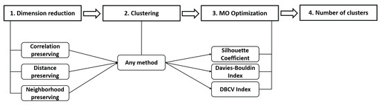
Figure 2.
A step-wise summary of the proposed method.
The process of transforming the dimensions is not studied here. It is assumed that the dimension reduction with suitable parameters is feasible, and the parameter selection for DR (if needed) is performed based on available studies or other heuristics. All the dimension reduction techniques have been used to obtain 2D data sets. All five mentioned DR techniques have been applied paired with each clustering, so for each data set, there are six versions available in total. More DR techniques can be used, and this number has been selected as a minimum. In addition, all four categories of previously mentioned clustering (seven methods in total) were utilized for a more thorough study.
As mentioned, in order to emphasize the unsupervised nature of this study, only internal metrics are considered for optimization, and the calculation of any external metrics is solely for the purpose of result comparison. These internal metrics are the Silhouette coefficient, DB and DBCV indices. The first two are to be maximized, but for the latter metric, lower values indicate better performance. Moreover, the DB index, in the context of this study, is in the order of 1000, while other indices are between 0–1. Therefore, the reciprocal of the DB index is maximized in the optimization process to uniformly maximize all the metrics in the same range.
After Pareto optimization, the number of presented solutions varies among different clustering methods and different dimension-reduced data sets. In some cases, the number of Pareto solutions is very high, and sometimes only a handful of solutions are acceptable. Hence, in order to balance the number of presented solutions in each case and remove the solutions with the poorest performance, a filter is placed after the optimization step. This filter removes the solutions that have any internal score with an absolute value lower than 0.01. Since the closeness of the calculated scores to zero is an indicator of their poor performance, this value has been selected as a heuristic threshold to eliminate possible substandard solutions.
4. Results
In this section, the results of the study are presented in individual graphs. For each data set, the results are grouped based on the category of clustering methods (distance-based, centroid-based, distribution-based and density-based), resulting in four subplots. Each plot demonstrates the fraction of Pareto solutions representing different number of clusters. The plots contain the performance of each DR technique and the overall performance, considering all the Pareto front solutions found for the data set. In the end of each part, an example of the actual clustering with the calculated AMI and V-measure is presented. The final part of this section is dedicated to key findings and a discussion of the results.
4.1. Wine Data Set
As an example of the optimization outcome, a three-dimensional space is presented in Figure 3, which summarizes the solution set for the PCA-reduced wine data set, with metrics calculated using DBSCAN clustering. The figure shows all the solutions obtained for optimizing the three metrics: i.e., Silhouette coefficient, DB index and DBCV index. The solid dots are the dominated solutions, and the points marked with x are the non-dominated solutions (Pareto front). The threshold regions to remove the solutions with poor performance resulted in removing the points marked in red. As demonstrated, in this case, three non-dominated solutions were removed, and the rest of the Pareto front is considered in the cluster number detection to calculate the fraction of solutions suggesting each number of clusters.
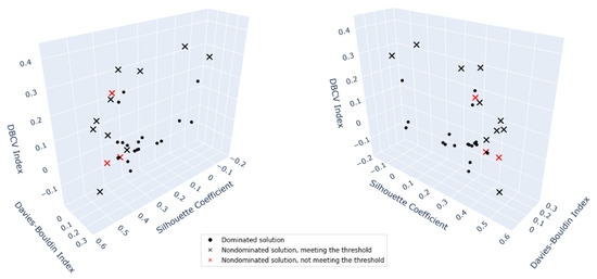
Figure 3.
A three-dimensional representation of the optimization space.
Different high-dimensional and low-dimensional versions of the data set suggest different numbers of clusters as their most repeated solution, while it should be kept in mind that each version presented a different number of Pareto front solutions. For example, as shown in Figure 4, for the distance-based category, all solutions found after ISOMAP dimension reduction suggested that there are two clusters present, and t-SNE results indicated that there are equal possibilities for the presence of three clusters and four clusters. Therefore, considering all the solutions overall leaves out the effects of each individual DR technique and helps us to examine the features of the data set that persisted throughout all the high-dimensional and low-dimensional versions, i.e., the number of clusters.
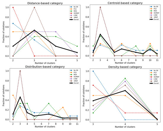
Figure 4.
Fraction of solutions representing found number of clusters in the wine data set for each DR technique.
Figure 4 indicates that, considering distance-based clustering methods, which include agglomerative hierarchical clustering, 0.53 of the solutions suggest that there are three clusters in the data set. For the centroid-based clustering, i.e., considering both k-means and k-medoids, this number is 0.44, and for the distribution-based category including GMM, this fraction is 0.46. Density-based methods, DBSCAN, OPTICS and HDBSCAN considered all together suggest four clusters in 0.60 of their solutions. It can be seen that first three categories of clustering methods detected 3 clusters, the expected number of clusters, and the last category detected four clusters. It should be noted that the methods in the final category are able to isolate outliers, hence ending up with expected number of clusters+1. Although no outliers were reported explicitly in this particular data set, some points were not assigned to any of the clusters, suggesting this possibility.
The selection of a solution from the Pareto set is called post-Pareto optimality analysis [44], which is not pursued in this work, but to observe an example of the clustering performance itself, one such solution is displayed in Figure 5. The data set is converted to two dimensions using ISOMAP, and clustering is performed using GMM. Different colors represent the clusters found by the method, and the true labels are marked with different shapes. The AMI obtained by this solution is 0.833 and the V-measure is 0.835, indicating a satisfactory outcome.
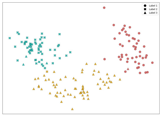
Figure 5.
GMM clustering of the wine data set with Isomap dimension reduction.
4.2. Synthetic Data Set
For this data set, Figure 6 shows how each clustering method performed in the determination of the number of clusters. The distance-based category suggests five clusters with 0.50 of the solutions, the centroid based suggests five clusters with 0.46 of the solutions, and distribution-based category indicates five clusters with 0.38 of the solutions. In all these cases, the cluster number with the highest fraction of the solutions does not have the majority (more than half), but it is the most-repeated outcome compared to others. On the other hand, the density-based category suggests six clusters with 0.76 of the solutions. The first three categories correctly detect five clusters in the data set, the same as the expected number of clusters. For the last category (three methods), the proposed approach suggests that there are six clusters in total, including the cluster of outliers. Again, the final results are consistent with the expected number of clusters + 1. In the first three plots, there are no solutions with more than five clusters, meaning that no non-dominated solutions detected more than five clusters.
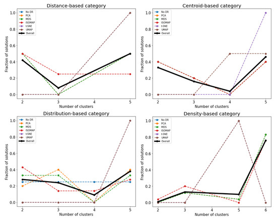
Figure 6.
Fraction of solutions representing the found number of clusters in the synthetic data set for each DR technique.
An example of clustering performance for this data set is demonstrated in Figure 7. The DR technique is MDS, and clustering is performed using DBSCAN. The five obtained clusters are in different colors, with the outliers in gray. The true labels are marked with different shapes, and the AMI for this clustering result is 0.835 and the V-measure is 0.835.
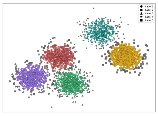
Figure 7.
DBSCAN clustering of the synthetic data set with MDS dimension reduction.
4.3. TEP Data Set
For the final data set, it can be seen in Figure 8 that the distance-based category suggests the presence of three clusters or nine clusters, each with a 0.16 probability, the centroid-based suggests eight clusters with 0.16 probability, and the distribution-based category suggests eight clusters with 0.16 and three clusters with 0.15 probability. In the last category—density-based—the final number is presented with a higher confidence compared to other categories, which is three clusters with 0.37 of all solutions.
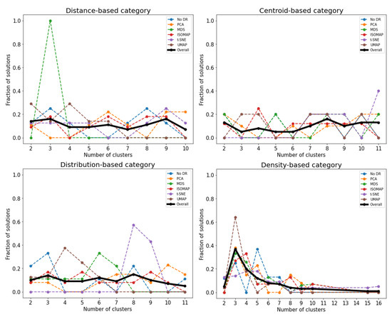
Figure 8.
Fraction of solutions representing found number of clusters in the TEP data set for each DR technique.
Based on what was noted for the expected number of clusters for this data set, the density-based category performed well. The final results indicate three clusters, which is equal to the expected number of clusters. Another category that suggested the presence of three clusters in the data set, but with a much lower confidence, was the distance-based category. This is in agreement with the results of [43] demonstrating that this category had the second-best performance in state isolation. From one of the solutions, the clusters found using hierarchical clustering on the t-SNE reduced data are presented in Figure 9, with an AMI of 0.766 and V-measure of 0.767. As it can be seen in this figure, the normal state and Fault 14 are combined in one cluster in yellow.
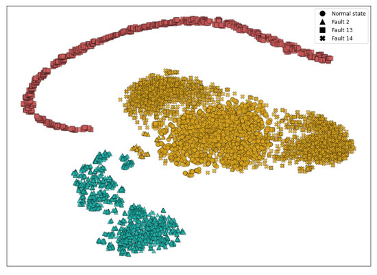
Figure 9.
Hierarchical clustering of the TEP data set with t-SNE dimension reduction.
4.4. Discussion of Results
Overall, this method demonstrates an outstanding performance in the determination of the number of clusters present in a data set. Key observations and further discussion of the results are provided below:
- Using any method that is not from the density-based category, the expected number of clusters is obtained. In cases where the density-based category detects one cluster more than the other categories, the final number can be interpreted as expected number of clusters + 1.
- In cases where different categories present inconsistent results, there is a possibility that an elongated cluster is present. In this case, further examination of the original data set and its lower-dimensional versions is needed to choose the final number of clusters.
- With all the attempts emphasizing carrying out all the steps in an unsupervised manner, in the end, the selection of the final number depends on a level of familiarity with the data set and/or the method as mentioned. A basic knowledge is required to decide whether the final number is with or without the outliers depending on the method and whether any number of clusters have overlapped during the DR or not. It should be noted that the required level of information can be easily obtained by the visualization of the dimensionally-reduced versions of the data set, since these features can be pointed out in the comparison of the different versions.
- Despite the advantages of overall consideration of solutions in finding the number of clusters in a data set, it can be interesting and beneficial to look at the individual performances of DR techniques in detecting the clusters. As seen in Figure 4, for all categories of clusterings, MDS, t-SNE and UMAP were the DR techniques that suggested the expected number of clusters, either with the highest probability or one of highest probabilities. For the synthetic data set in Figure 6, it is demonstrated that t-SNE and UMAP lead to the same results as the overall performance in three out of four clustering categories, with the exception of the density-based category. The performance of PCA and MDS is consistent with the overall performance in another three out of four clustering categories, with the exception being the distribution-based methods. For the case with an elongated cluster, by looking at the density-based category in Figure 8, PCA, MDS and UMAP suggest the same number of clusters as the overall performance. In conclusion, UMAP can deliver satisfactory results in almost every case. In the quantitative survey on DR techniques by [5], UMAP was also suggested as one of the techniques yielding the best quality of projection based on their considered quality metrics.
- Considering the no DR solutions obtained for each clustering category, there is no specific pattern of behavior in the results of the wine data set and TEP data set, and the clustering of the original data set was only able to detect the number of clusters in at most two categories, still not with a high probability compared to other numbers. However, the clustering of the original data set for the synthetic data led to the same result in terms of the overall performance. This can be explained by the dimensionality of the data at hand. The synthetic data set was two-dimensional, while the other data sets were high-dimensional, and in the latter, clustering methods utilizing traditional distance measures, such as Euclidean, may be ineffective in detecting the clusters, since such distance measures may be dominated by noise in many dimensions [45].
4.5. Observations
One of the key assumptions of the present work is the existence of true/ideal cluster labels. While for most real-life motivated examples, this can be true, they would often be unknown to the analysts. Therefore, the parametrization of classification algorithms should be directed towards the capture of underlying features of the dataset. In most cases, however, the driving mechanism of the cluster formulation is opaque; the clusters can be revealed by the assumption of centrality, density, connectivity, etc. The associated evaluation metrics are of similar diversity. As a result, the parametrization methodology proposed in this work aims to incorporate as many of these assumptions as possible to create a more agnostic conceptualization. Interestingly, one can clearly observe that two different clustering solutions yield similarly good or even outstanding metrics, yet neither may describe the true/ideal structure of the dataset. This is an inherent problem of unsupervised learning algorithms, where the global optimality is often hard to locate if not impossible to be proved. The multi-objective formulation helps to address this shortcoming, at least in principle.
Another issue is the potential existence of conflicting performance metrics as the general assumption of the definition of Pareto fronts. However, the different dimension reduction, clustering and performance measurement techniques are generally not in conflict with each other in terms of their performance metrics. Nevertheless, these solutions still constitute the best available in the addressed search space, and therefore the associated parameter sets are the best available for the analyst.
A third issue is that the traditional clustering algorithms do not aim to directly optimize the proposed performance metrics. Therefore, we should be able to directly define new clustering algorithms explicitly aiming for the optimization of these performance metrics. Our aim, however, was not the formalization of new clustering algorithms but to support the parametrization of existing, well-known approaches.
Finally, we note that global optimality is challenging to mathematically formulate, especially in domains where often a high proportion of domain knowledge is required by experts during the analysis of the results. While there is clearly room for future developments in this field, the proposed methodology provides a an acceptable, practical and insightful solution to the problem.
5. Conclusions
In exploring and extracting information from high-dimensional data sets, clustering plays an important role. Most of the clustering methods need some information about internal features of the data set, if not the actual number of clusters. In order to utilize clustering as an unsupervised data analysis tool, a method has been proposed in this study to simultaneously optimize a number of internal cluster validation metrics to detect the number of clusters present in the data. This process is also carried out on dimensionally reduced versions of the data set, since it is assumed that the most important features of the data will be preserved after dimension reduction. This approach was carried out on three data sets with distinct features. In all three cases, the approach was able to correctly detect the expected number of clusters, and it is important to mention that the results were achievable irrespective of the selection of the clustering method. Besides the determination of the optimally applied cluster number parameter, our key observations underpinned previous findings of the quantitative survey on DR techniques that UMAP can deliver satisfactory results in almost every case. Moreover, according to our results, in the case of high-dimensional data sets, clustering methods utilizing traditional distance measures, such as Euclidean, may be ineffective in detecting the clusters, since such distance measures may be dominated by noise in many dimensions. Overall, this method can be a useful step to detect the number of clusters in a data set as it requires no or basic preliminary examinations of features of the data.
Author Contributions
Conceptualization, M.M., G.D. and A.P.; methodology, M.M., G.D. and A.P.; formal analysis, M.M.; investigation, M.M.; data curation, M.M.; writing—original draft preparation, M.M.; writing—review and editing, G.D. and A.P.; visualization, M.M.; supervision, A.P.; project administration, A.P. All authors have read and agreed to the published version of the manuscript.
Funding
This research received no external funding.
Institutional Review Board Statement
Not applicable.
Data Availability Statement
The data that support the findings of this study are available from the corresponding author, M.M., upon reasonable request.
Acknowledgments
G.D. thankfully acknowledges the financial support of the Fulbright Scholarship, which made his year at the University of California, Davis possible and founded a collaboration between the research groups. G.D. was supported by the doctoral student scholarship program of the Co-operative Doctoral Program of the Ministry of Innovation and Technology financed by the National Research, Development and Innovation Fund, Hungary.
Conflicts of Interest
The authors declare no conflict of interest.
References
- Qin, S. Statistical process monitoring: Basics and beyond. J. Chemom. J. Chemom. Soc. 2003, 17, 480–502. [Google Scholar]
- Qin, S. Survey on data-driven industrial process monitoring and diagnosis. Annu. Rev. Control 2012, 36, 220–234. [Google Scholar] [CrossRef]
- Ming, L.; Zhao, J. Review on chemical process fault detection and diagnosis. In Proceedings of the 2017 6th International Symposium on Advanced Control of Industrial Processes (AdCONIP), Taipei, Taiwan, 28–31 May 2017; pp. 457–462. [Google Scholar] [CrossRef]
- Zheng, S.; Zhao, J. A new unsupervised data mining method based on the stacked autoencoder for chemical process fault diagnosis. Comput. Chem. Eng. 2020, 135, 106755. [Google Scholar] [CrossRef]
- Espadoto, M.; Martins, R.M.; Kerren, A.; Hirata, N.S.T.; Telea, A.C. Towards a Quantitative Survey of Dimension Reduction Techniques. IEEE Trans. Vis. Comput. Graph. 2019, 27, 2153–2173. [Google Scholar] [CrossRef]
- Xu, D.; Tian, Y. A Comprehensive Survey of Clustering Algorithms. Ann. Data Sci. 2015, 2, 165–193. [Google Scholar] [CrossRef]
- Quiñones-Grueiro, M.; Prieto-Moreno, A.; Verde, C.; Llanes-Santiago, O. Data-driven monitoring of multimode continuous processes: A review. Chemom. Intell. Lab. Syst. 2019, 189, 56–71. [Google Scholar] [CrossRef]
- Nor, N.; Hassan, C.R.C.; Hussain, M.A. A review of data-driven fault detection and diagnosis methods: Applications in chemical process systems. Rev. Chem. Eng. 2020, 36, 513–553. [Google Scholar] [CrossRef]
- Thomas, M.C.; Zhu, W.; Romagnoli, J.A. Data mining and clustering in chemical process databases for monitoring and knowledge discovery. J. Process Control. 2018, 67, 160–175. [Google Scholar] [CrossRef]
- Palacio-Niño, J.; Berzal, F. Evaluation Metrics for Unsupervised Learning Algorithms. arXiv 2019, arXiv:1905.05667. [Google Scholar]
- Zimmermann, A. Method evaluation, parameterization, and result validation in unsupervised data mining: A critical survey. Wiley Interdiscip. Rev. Data Min. Knowl. Discov. 2020, 10, e1330. [Google Scholar] [CrossRef]
- Milligan, G.W.; Cooper, M.C. An examination of procedures for determining the number of clusters in a data set. Psychometrika 1985, 50, 159–179. [Google Scholar] [CrossRef]
- Van Craenendonck, T.; Blockeel, H. Using internal validity measures to compare clustering algorithms. In Proceedings of the Benelearn 2015 Poster Presentations (Online), AutoML Workshop at ICML 2015, Delft, The Netherlands, 19 June 2015; pp. 1–8. [Google Scholar]
- Ngatchou, P.; Zarei, A.; El-Sharkawi, A. Pareto Multi Objective Optimization. In Proceedings of the 13th International Conference on, Intelligent Systems Application to Power Systems, Arlington, VA, USA, 6–10 November 2005; pp. 84–91. [Google Scholar] [CrossRef]
- Mishra, S.; Saha, S.; Mondal, S. Unsupervised method to ensemble results of multiple clustering solutions for bibliographic data. In Proceedings of the 2017 IEEE Congress on Evolutionary Computation, Donostia, Spain, 5–8 June 2017; pp. 1459–1466. [Google Scholar]
- Mukhopadhyay, A.; Maulik, U.; Bandyopadhyay, S. A survey of multiobjective evolutionary clustering. ACM Comput. Surv. 2015, 47, 1–46. [Google Scholar] [CrossRef]
- Handl, J.; Knowles, J. Exploiting the trade-off—The benefits of multiple objectives in data clustering. In Proceedings of the International Conference on Evolutionary Multi-Criterion Optimization, East Lansing, MI, USA, 10–13 March 2005; Springer: Berlin/Heidelberg, Germany, 2005; pp. 547–560. [Google Scholar]
- Bandyopadhyay, S.; Maulik, U.; Mukhopadhyay, A. Multiobjective genetic clustering for pixel classification in remote sensing imagery. IEEE Trans. Geosci. Remote Sens. 2007, 45, 1506–1511. [Google Scholar] [CrossRef]
- Emmerich, M.T.; Deutz, A.H. A tutorial on multiobjective optimization: Fundamentals and evolutionary methods. Nat. Comput. 2018, 17, 585–609. [Google Scholar] [CrossRef]
- Cinar, A.; Palazoglu, A.; Kayihan, F. Chemical Process Performance Evaluation; CRC Press: Boca Raton, FL, USA, 2007. [Google Scholar]
- Pearson, K.F. LIII. On lines and planes of closest fit to systems of points in space. Lond. Edinb. Dublin Philos. Mag. J. Sci. 1901, 2, 559–572. [Google Scholar] [CrossRef]
- Torgerson, W.S. Theory and Methods of Scaling; Wiley: Hoboken, NJ, USA, 1958. [Google Scholar]
- Tenenbaum, J.B.; De Silva, V.; Langford, J.C. A global geometric framework for nonlinear dimensionality reduction. Science 2000, 290, 2319–2323. [Google Scholar] [CrossRef] [PubMed]
- Van der Maaten, L.; Hinton, G. Visualizing data using t-SNE. J. Mach. Learn. Res. 2008, 9, 2579–2605. [Google Scholar]
- McInnes, L.; Healy, J.; Melville, J. Umap: Uniform manifold approximation and projection for dimension reduction. arXiv 2018, arXiv:1802.03426. [Google Scholar]
- Zepeda-Mendoza, M.L.; Resendis-Antonio, O. Hierarchical agglomerative clustering. Encycl. Syst. Biol. 2013, 43, 886–887. [Google Scholar]
- MacQueen, J. Some methods for classification and analysis of multivariate observations. In Proceedings of the 5th Berkeley Symposium on Mathematical Statistics and Probability, Oakland, CA, USA, 18–21 July 1967; Volume 1, pp. 281–297. [Google Scholar]
- Park, H.S.; Jun, C.H. A simple and fast algorithm for K-medoids clustering. Expert Syst. Appl. 2009, 36, 3336–3341. [Google Scholar] [CrossRef]
- Rasmussen, C.E. The infinite Gaussian mixture model. NIPS 1999, 12, 554–560. [Google Scholar]
- Ester, M.; Kriegel, H.P.; Sander, J.; Xu, X. A density-based algorithm for discovering clusters in large spatial databases with noise. Kdd 1996, 96, 226–231. [Google Scholar]
- Ankerst, M.; Breunig, M.M.; Kriegel, H.P.; Sander, J. OPTICS: Ordering points to identify the clustering structure. ACM Sigmod Rec. 1999, 28, 49–60. [Google Scholar] [CrossRef]
- McInnes, L.; Healy, J.; Astels, S. hdbscan: Hierarchical density based clustering. J. Open Source Softw. 2017, 2, 205. [Google Scholar] [CrossRef]
- Vinh, N.X.; Epps, J.; Bailey, J. Information theoretic measures for clusterings comparison: Variants, properties, normalization and correction for chance. J. Mach. Learn. Res. 2010, 11, 2837–2854. [Google Scholar]
- Rosenberg, A.; Hirschberg, J. V-measure: A conditional entropy-based external cluster evaluation measure. In Proceedings of the 2007 Joint Conference on Empirical Methods in Natural Language Processing and Computational Natural Language Learning (EMNLP-CoNLL), Prague, Czech Republic, 28–30 June 2007; pp. 410–420. [Google Scholar]
- Rousseeuw, P.J. Silhouettes: A graphical aid to the interpretation and validation of cluster analysis. J. Comput. Appl. Math. 1987, 20, 53–65. [Google Scholar] [CrossRef]
- Davies, D.L.; Bouldin, D.W. A cluster separation measure. IEEE Trans. Pattern Anal. Mach. Intell. 1979, 2, 224–227. [Google Scholar] [CrossRef]
- Dunn, J.C. Well-separated clusters and optimal fuzzy partitions. J. Cybern. 1974, 4, 95–104. [Google Scholar] [CrossRef]
- Caliński, T.; Harabasz, J. A dendrite method for cluster analysis. Commun. Stat.-Theory Methods 1974, 3, 1–27. [Google Scholar] [CrossRef]
- Moulavi, D.; Jaskowiak, P.A.; Campello, R.J.; Zimek, A.; Sander, J. Density-based clustering validation. In Proceedings of the 2014 SIAM International Conference on Data Mining, Philadelphia, PA, USA, 24–26 April 2014; pp. 839–847. [Google Scholar]
- Dua, D.; Graff, C. UCI Machine Learning Repository; University of California, School of Information and Computer Science: Irvine, CA, USA, 2019; Volume 25, p. 27. [Google Scholar]
- Pedregosa, F.; Varoquaux, G.; Gramfort, A.; Michel, V.; Thirion, B.; Grisel, O.; Blondel, M.; Prettenhofer, P.; Weiss, R.; Dubourg, V.; et al. Scikit-learn: Machine Learning in Python. J. Mach. Learn. Res. 2011, 12, 2825–2830. [Google Scholar]
- Bathelt, A.; Ricker, N.L.; Jelali, M. Revision of the Tennessee Eastman Process Model. IFAC-Pap. Online 2015, 48, 309–314. [Google Scholar] [CrossRef]
- Mollaian, M.; Dörgő, G.; Palazoglu, A. Studying the Synergy between Dimension Reduction and Clustering Methods to Facilitate Fault Classification. In Computer Aided Chemical Engineering, Proceedings of the 31st European Symposium on Computer Aided Process Engineering, Istanbul, Turkey, 6–9 June 2021; Türkay, M., Gani, R., Eds.; Elsevier: Amsterdam, The Netherlands, 2021; Volume 50, pp. 819–824. [Google Scholar]
- Carrillo, V.M.; Aguirre, O.; Taboada, H. Applications and performance of the non-numerical ranking preferences method for post-Pareto optimality. Procedia Comput. Sci. 2011, 6, 243–248. [Google Scholar] [CrossRef][Green Version]
- Han, J.; Kamber, M.; Pei, J. Data Mining Concepts and Techniques, 3rd ed.; Elsevier: Amsterdam, The Netherlands, 2011; Volume 5. [Google Scholar]
Publisher’s Note: MDPI stays neutral with regard to jurisdictional claims in published maps and institutional affiliations. |
© 2022 by the authors. Licensee MDPI, Basel, Switzerland. This article is an open access article distributed under the terms and conditions of the Creative Commons Attribution (CC BY) license (https://creativecommons.org/licenses/by/4.0/).