Abstract
In order to further improve the efficiency and economic benefits of multi-stage fracturing of unconventional oil and gas horizontal wells, it is urgently needed to conduct comprehensive reservoir quality evaluation research on the whole horizontal well section. Firstly, based on logging data, focusing on reservoir quality and completion quality, and comprehensively considering key factors such as reservoir physical property indexes and fracability indexes, a subjective and objective coupled evaluation model of the entropy weight method (EWM) and the analytic hierarchy process (AHP) without bias is established to obtain the composite reservoir quality index. Then, unsupervised gaussian mixture model (GMM) clustering algorithms are used to classify the reservoir comprehensive quality index and finally four grades of fracturing stages are established. Taking shale oil well A and B of the Permian Lucaogou Formation in Jimsar Sag, Junggar Basin, as examples, the comprehensive reservoir quality evaluation and clustering model training, testing, and prediction were carried out. By comparing the clustering results with the actual fracturing stages and oil production, it is found that the evaluation results obtained by the GMM clustering algorithms based on the coupled evaluation model of EWM and AHP can identify the good fracturing grades. The algorithm can also predict the fracturing grades of other wells in the same block. It proves the accuracy of the method proposed in this paper and provides a favorable technical basis for determining the placement of multi-cluster fracturing perforation.
1. Introduction
Currently, most unconventional reserves are characterized by a low grade, low and ultra-low permeability resources, and high commercial development costs [1]. Reservoir optimization evaluation and multi-stage fracturing are key technologies to reduce costs and increase efficiency in unconventional oil and gas development [2,3,4]. However, there are many indicators involved in reservoir optimization evaluation and inaccurate quantification [5,6], and when in multi-stage perforation fracturing, unreasonable selection of the fracturing stages leads to low production after fracturing [7,8]. Therefore, to define the basis of multi-stage and multi-cluster division of the horizontal wells, and to solve the problems of low accuracy and poor operability in the evaluation of reservoir quality and completion quality, we need to establish a set of comprehensive methods of evaluation based on well logging and mud logging data; this will realize being comprehensive and unify the evaluation parameters, as well as self-adaptive multi-stage optimization, to meet the demands of practical and efficient engineering applications.
Previously, domestic and foreign scholars have carried out some studies on reservoir evaluation. For example, Roberto et al. [9,10] considered the reservoir quality composed of hydrocarbon-filled porosity, permeability, pore pressure, organic carbon content, and organic maturity, and the completion quality composed of fracture height growth and fracability. Zou et al. [11] focused on the matching evaluation of the “six characteristics” of hydrocarbon source, lithology, physical property, brittleness, hydrocarbon potential, and stress anisotropy, and proposed eight evaluation criteria for unconventional oil and gas enrichment areas. Scholars at home and abroad have also carried out relevant studies on the optimization design of the fracturing stage. Lei et al. [12] proposed a geological engineering integrated reservoir reconstruction design platform, and the pre-fracture analysis module selected the fracturing well stage through comprehensive evaluation of reservoir quality and completion quality. Liu et al. [13] proposed stratigraphic modeling and evaluation technology for horizontal wells, integrating anisotropic reservoir quality evaluation and engineering quality evaluation methods such as in situ stress and brittleness to identify the sweet spot section of the horizontal wells and fracability, and finally optimized the horizontal well segmentation by integrating the stress and lithologic interval. Zhang et al. [14] used the unsupervised clustering algorithms based on Euclidean distance to cluster the reservoir according to reservoir flow and geomechanical parameters, and identified the fracability area of the fractured section of the reservoir so as to ensure the effectiveness of the perforation fracturing and improve the efficiency of the perforation fracturing. Slocombe et al. [15] compared fracture stages divided by engineering and geometric methods and found that effective stimulation was achieved by grouping formations with similar stress in engineering fracture stages. Cipolla et al. and Atanayev et al. [16,17,18] divided the well into several stages based on reservoir quality and completion quality by subjectively assigning quality evaluation and setting thresholds. Ejofodomi and Salah [19,20], based on Cipolla’s work, considered an anisotropic one-dimensional geomechanical model of a reservoir for completion quality, which improved the fracturing efficiency. Starting from the sweet spot evaluation of horizontal well engineering, Li et al. [21] comprehensively considered the factors of reservoir fracability indexes, physical property indexes, the fracture-induced stress field, and fracture pressure profile to divide the fracturing stages. Xia et al. [22] used the grey correlation analysis and multi-correlation coefficient method to evaluate the reservoir based on the characteristic quality of source rock, reservoir physical quality, and completion quality.
To sum up, for reservoir evaluation, foreign scholars usually use reservoir quality and completion quality to evaluate the reservoirs quantitatively through the subjective weighting method, with reservoir quality corresponding well with the reservoir physical properties such as high gas richness and high organic content, and completion quality corresponding to the reservoir’s good fracability; in turn, domestic scholars evaluates the six characteristics of source rock quality, completion quality, and reservoir physical quality to evaluate a reservoir by the objective weighting method. There are many evaluation indicators considered comprehensively by scholars at home and abroad, but it is difficult to evaluate reservoir quantitatively by unifying them, and the subjective and objective weighting methods are not combined to comprehensively evaluate a reservoir. As for the optimization design of fracturing stages, there are mainly geometric and engineering staging methods, where geometric staging means equal spacing of the perforating clusters. Because of the low production of the fracturing stages caused by geometric staging, this paper mainly discusses the engineering staging of the fracturing stages based on quality design. Most scholars divide the fracturing stages by subjectively setting thresholds based on the integration of geology and engineering, which has disadvantages such as strong subjectivity and poor operation. Some scholars considered the clustering algorithm based on Euclidean distance to improve the efficiency of the fracturing staging. This method has the problem of poor clustering, a result of non-spherical data sets. Therefore, this paper puts forward three quality evaluation methods—the reservoir quality, completion quality, and composite quality of the reservoir—and evaluates the three qualities of the reservoir based on the unbiased subjective and objective, coupled evaluation models of the entropy weight method and analytic hierarchy process. Then, unsupervised machine learning GMM clustering algorithms were used to classify the well segments and identify the fracturing, which provides a key technical support for multi-cluster fracturing and perforating.
2. Methodology
2.1. Calculation of Three Quality Indexes Based on Logging Data
Reservoir quality and completion quality are the keys to characterize the physical properties and fracability of the reservoir, and provide a basis for the later optimization of multi-stage and multi-cluster fracturing perforation; so, this article is based on well logging, such as the natural gamma ray, natural potential, density, and interval transit time, to extract the reservoir quality, completion quality, and composite quality index. The specific method is as follows.
2.1.1. Calculation of Reservoir Quality Index
The reservoir quality index is the main basis for logging the interpretation classification and fracturing fault selection, and the physical property of the reservoir is the main influencing factor, including the shale content, porosity, permeability, and oil saturation.
(1) For the calculation of effective porosity, the shale content is obtained according to the natural gamma ray and natural potential logging curves, and then the effective porosity is calculated by the Wylie formula.
where is the effective porosity, %; is the interval transit time logging value of the target layer; is the interval transit time of rock skeleton, ; is the interval transit time of formation fluid, ; is the shale content of formation, decimal; and is the interval transit time of shale, .
(2) The permeability calculation, based on the known porosity of Equation (1), Zeng [23] proposed a statistical empirical formula to obtain the permeability.
(3) The calculation of oil saturation is obtained by the Archie formula [24].
2.1.2. Calculation of the Completion Quality Index
Completion quality mainly considers the fracability of the reservoir and is used to characterize the difficulty of effective fracturing, including six evaluation indicators: the brittleness index, fracture toughness index, horizontal stress difference index, vertical stress difference index, natural fracture index, and bedding development index.
(1) Many scholars at home and abroad have done a lot of research on the calculation of the brittleness index. This paper mainly refers to the mineral content brittleness index method proposed by Jin et al. [25], the mechanical brittleness index method proposed by Rickman et al. [26], and the energy-based brittleness index method proposed by Ning Li et al. [27].
where is mineral brittleness index, dimensionless; is the mechanical brittleness index of rock, dimensionless; is brittleness index of energy evolution, dimensionless; and are the weight values of each evaluation index to evaluate the brittleness index, dimensionless.
(2) The fracture toughness index is an important factor affecting the difficulty of the fracturing and reflects the ability of maintaining the fracture extension after fracture formation in the fracturing process. The calculation formula in this paper refers to the fracture toughness formula determined by Jin Yan et al. [28,29] using the multiple nonlinear regression method.
where is the fracture toughness, ; and are the maximum and minimum fracture toughness, respectively, .
(3) The horizontal stress difference index is the difference between the maximum horizontal principal stress and the minimum horizontal principal stress, which is mainly affected by tectonic movement. Based on the transverse isotropic model [30], the calculation formula is as follows:
where is the horizontal stress difference value, , ; is the corresponding threshold of horizontal stress difference when forming hydraulic fractures; ; and is the corresponding threshold of horizontal stress difference when the ideal hydraulic fractures is formed, .
(4) The vertical stress difference index is the difference between vertical stress and the minimum horizontal principal stress. Its calculation formula is as follows:
where is the vertical stress difference, , ; is the corresponding vertical stress difference threshold when simple vertical fractures are formed by fracturing, ; is the vertical stress difference threshold corresponding to the formation of simple bedding fractures during fracturing, ; and is the optimal vertical stress difference value for forming the complex fractur network, .
(5) For the natural fracture index calculation, the harmonic mean method is adopted to consider the influence of the natural fracture length, natural fracture density, and angle between the natural fracture orientation and horizontal maximum principal stress direction on fracability. The specific formula is as follows:
where is the normalized natural fracture length, ; is the maximum natural fracture length, ; is the minimum natural fracture length, ; is the normalized natural fracture density line; is maximum fracture density, line; is minimum fracture density, line; is the angle between the natural fracture and horizontal maximum principal stress direction, degree; and is the angle between normalized natural fracture orientation and horizontal maximum principal stress direction.
(6) Calculation of the bedding development index.
where is the bedding density; is the optimal bedding density; is the bedding density threshold corresponding to the fracture morphology dominated by forming bedding; and is the corresponding bedding density threshold when forming a fracture morphology dominated by hydraulic fractures.
2.1.3. Calculation of the Composite Quality Index
(1) Normalization of the original data
Due to the different physical meanings of various indicators for reservoir evaluation, normalization should be carried out before calculating the composite quality index, which can eliminate the influence of differences in the magnitude of absolute values of different parameters on the evaluation effect. The specific methods are as follows.
Suppose there is evaluation parameter indicators, and each evaluation parameter indicator has evaluation objects; then, the original data of the corresponding indicator of the evaluated object can be expressed as by the following matrix, and the calculation is as follows:
Positive indictors:
Negative indictors:
where is the parameters of the th evaluation object of the th evaluation indicator after normalization, dimensionless; and is the parameter of the th evaluation object of the th evaluation indicator of original data (; ).
(2) Calculation of the reservoir quality index:
where is reservoir quality index, dimensionless; is the parameter value after normalization of the th reservoir quality evaluation indicator, dimensionless; is the weight of the th indicators, .
(3) Calculation of the reservoir quality index:
where is completion quality index, dimensionless; and is the weight of the th indicator of completion quality, dimensionless, .
(4) The composite quality index takes into account both reservoir quality and completion quality, and selects the best completion quality interval for fracturing. Then, the composite quality index of reservoir can be calculated as follows:
where is the composite quality index of reservoir, dimensionless; and and are the weight values of and , dimensionless.
2.2. Coupled Evaluation Model of the Entropy Weight Method and Analytic Hierarchy Process
Based on the three quality indexes for the evaluation of the reservoir physical property and fracability, the core problem is the determination of the indicator weight. At present, the main weight calculation methods include subjective, objective, and combined weight methods [31]. The subjective weight method converts the subjective preferences of decision-makers into actual evaluation values, reflecting the leading role of the decision-makers, while the objective weight method completely relies on objective data information, completely abandoning the subjective initiative of the decision-makers and lacks flexibility in the decision-making process. Due to the complexity of unconventional oil and gas reservoirs, the subjective and objective weighting methods are often needed to comprehensively evaluate the reservoir, and finally optimize the subjective and objective weighting value. Therefore, this paper proposes a coupled evaluation model using the entropy weighting method and analytic hierarchy process.
2.2.1. The Entropy Weight Method (EWM)
EWM is based on the difference between the same indicators in the original data as the basis for weight determination [32]. The greater the difference between the evaluation indicators, the smaller the entropy value, and the more information this indicator contains and transmits, the greater the weight of the information obtained. Such methods are less affected by subjective factors, and different samples will have different weight values. For unconventional reservoirs with strong heterogeneity and large differences in physical properties, EWM can be combined with a variety of reservoir evaluation indicators to comprehensively weight the samples, so that the weights of different indicators are independent of each other, and only reflect the characteristics of strong or weak heterogeneity of the reservoir evaluation indicators, which can better realize the comparison of differences among the sample indicators. This method determines the weight value according to the relationship between the amount of information of the sample data and the probability of random events, which has a high calculation efficiency, and can be used to solve the weight value of the evaluation indicators more objectively.
Calculate the entropy weight of the th evaluation indicator:
where is the proportion of the th evaluation object of the th evaluation indicator, dimensionless; and is the entropy weight of the th evaluation indicator, dimensionless, and the weight vector is .
2.2.2. The Analytic Hierarchy Process (AHP)
AHP is a subjective weight method to specify the weight value according to the judgment of the decision-makers. For the establishment of the layer structure of different evaluation indicators, it is decomposed into elements, and the elements are divided into several groups according to their properties, forming different levels. AHP avoids the deficiency of the objective weighting method without subjective preference. The weight setting of each layer will eventually directly or indirectly affect the result, and the influence degree of each factor in each layer on the result is quantified, very clear, and explicit.
(1) The establishment of the judgment matrix
The judgment matrix represents the importance of elements at a certain layer relative to elements at the next layer, and nine scales are introduced [33]. If there are evaluation parameter indicators, and each evaluation parameter indicator has evaluation objects, the judgment matrix is established .
(2) The weight calculation (summation method)
where is the normalization of the th column vector of the judgment matrix, namely, ; is the weight value of the th evaluation parameter indicator, and the weight vector is .
(3) For the consistency test calculation [33], when , the judgment matrix is considered acceptable; otherwise, the judgment matrix should be modified appropriately.
2.2.3. Establishment of the Coupled Evaluation Model Entropy Weight Method and Analytic Hierarchy Process
In order to consider the shortcomings of the subjective and objective weights and minimize the total deviation between the evaluation results and the evaluation results under the subjective and objective weights, this paper adopts the quadratic programming method [34] to combine the subjective and objective weights without deviation. Establish the objective function:
where is the comprehensive weight value vector, ; is the matrix after the normalization of the original data, ; C is the unit row vector; and is an arbitrary constant.
Construct the Lagrange function for the objective function, getting
where is the Lagrange multiplier. Let , , the comprehensive weight value vector of the solution , where, , .
2.3. Gaussian Mixture Model (GMM) Clustering Algorithms
The classical k-means clustering algorithm often ends up with the local optimization of the SSE function of the clustering error, and is sensitive to noise and outliers [35,36]. It is not suitable for discovering non-spherical clusters or clusters with large size differences, and only applies to data sets with continuous attributes. However, the Gaussian mixture model (GMM) clustering algorithm is more flexible in processing data shapes than the k-means clustering algorithms [37,38], and the data set can be any non-spherical shape. GMM accurately quantifies a data set through a Gaussian probability density function by dividing the data set into several models based on the Gaussian probability density function. GMM is also the probability model with the fastest learning speed, which builds an appropriate linear GMM distribution combination model by fitting the input data set, so as to achieve the purpose of unsupervised clustering. Therefore, the characteristics of the spheroidal data set in this paper are suitable for clustering using the probability density model. GMM clustering algorithms are used to classify the reservoir composite quality, which makes the reservoir composite quality index of the same fracturing stage similar, and ensures that the reservoir quality and completion quality characteristics of the same clustering category are less different, while the reservoir quality and completion quality of different clustering categories are significantly different.
2.3.1. Standardization of Original Data
As the reservoir data changes with the depth of the formation, such original data sets fluctuate greatly, which will have a great impact on the clustering results. Therefore, in order to ensure that the data set is relatively stable and obeys a normal distribution, the Z-score method is adopted to standardize the composite quality index of the reservoir. Given samples and indicators, is the original data matrix, and the standardized transformation is
where is the average value of the th indicator; and is the variance of the th indicator.
2.3.2. GMM Clustering Algorithms
The sample data set of a known reservoir composite quality index conforms to a gaussian distribution; then, the GMM is as follows [39]:
where , and the unit gaussian distribution , with mean and covariance matrix , is called a component of the GMM, where is a mixed parameter, and is the weight of the gaussian distributions and represents prior probability:
The probability density function of is
2.4. Flowchart of the Identification of the Fracturing Grades
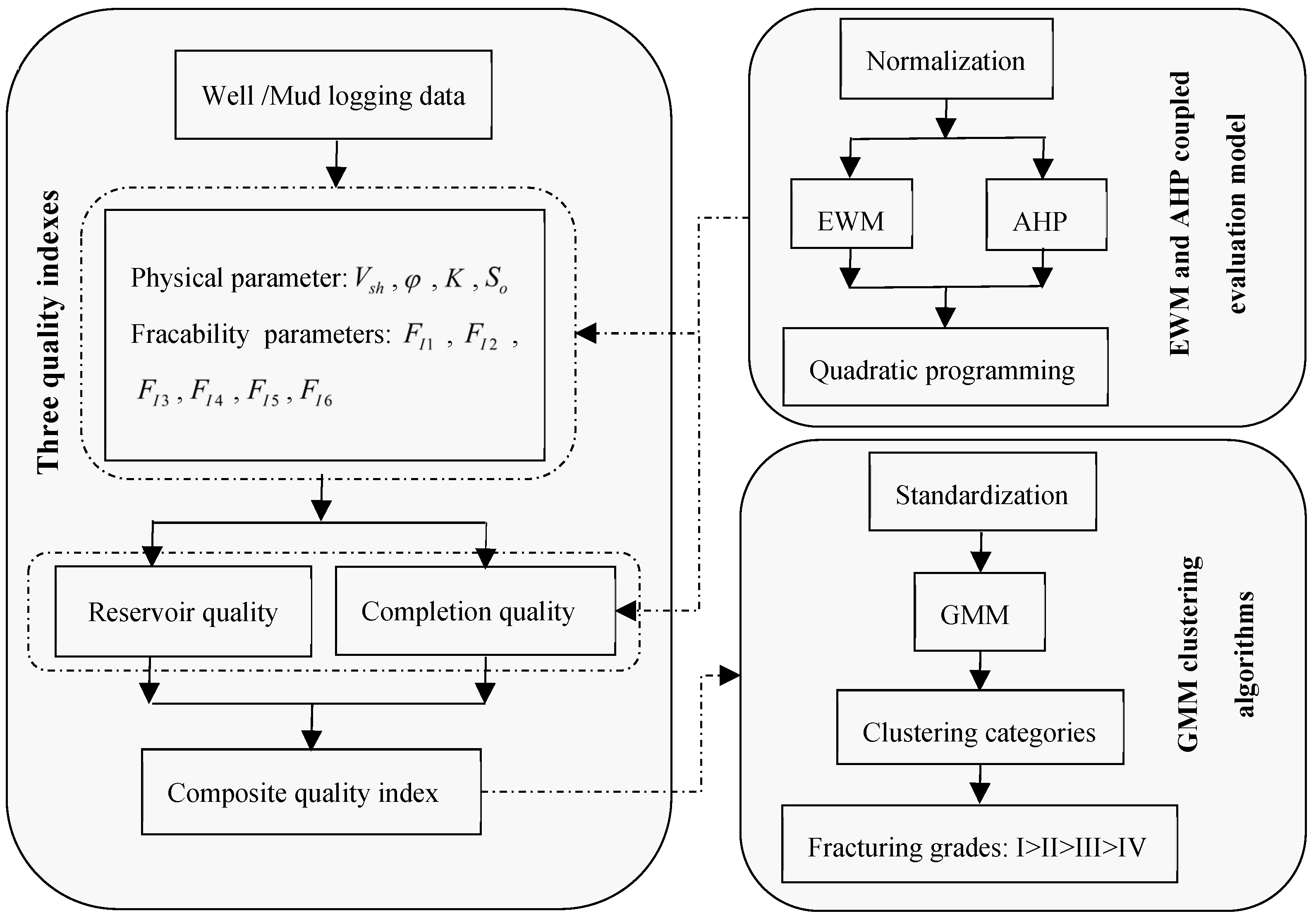
This paper is based on the logging or mud logging data to obtain the reservoir physical property parameters and fracability parameters, using the coupled evaluation model of EWM and AHP, for reservoir quality, completion quality, and composite quality evaluation; for the composite reservoir quality index for the division of the GMM clustering categories and identifying the grades of fracturing, the specific process is shown in Figure 1.
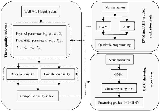
Figure 1.
Flowchart of identification of the fracturing grades based on the EWM–AHP coupled evaluation model and GMM clustering algorithms.
3. Case Study and Discussion
The horizontal section of well A selected in this paper is 4020.0~5725.0 m, and the reservoir porosity is 5.02~38.67%; the average porosity is 11.0%, the oil saturation is 45.0~100.0%, and the average oil saturation is 81.9%. The casing of the oil reservoir, with an outer diameter of 139.7 mm, is used for well completion. In the well section of 4020.0~5725.0 m, there are 15 stages, 145 clusters, a 981 m effective reconstruction section length, average cluster spacing of 6.8 m, and average segment spacing of 65.4 m. The interpreted horizontal section of well B is 4052.0~5718.0 m, the interpreted reservoir porosity is 0.12~31.3%, the average porosity is 7.7%, the oil saturation is 0.29~99.00%, and the average oil saturation is 63.9%. There are 103 clusters in 35 stages within the well section 4052.0~5718.0 m. The effective reconstructed section length is 915.5 m, the average cluster spacing is 15.8 m, and the average segment spacing is 48.3 m. After processing the cleaning data and outliers, this paper firstly selects the logging data of 4072.0–4472.0 m in well A to calculate the three quality indexes through the coupled evaluation model of EWM and AHP. Then the GMM clustering model was trained and classified by the composite quality index, and the clustering results were compared with the actual fracturing and oil production of the well section. Finally, the trained clustering model was used to predict and classify the reservoir quality of 4032.0–4506.0 m in well B and identify the grades of fracturing stages.
3.1. Analysis of the Coupled Evaluation Model of EMW and AHP
In this paper, the evaluation indicators of reservoir quality and completion quality were obtained based on logging data of well A, and the weight index of each indicator of reservoir quality and completion quality were obtained by EMW and AHP, respectively. Finally, the optimal comprehensive weight value was obtained by quadratic programming method.
As can be seen from Table 1, when calculating the weight of each evaluation indicator of reservoir quality, the AHP is based on the knowledge of the decision-maker on reservoir oil content, and is the most important, so the weight of oil saturation is the largest. According to the heterogeneity of the reservoir, the entropy weight of the shale content is small, so the weight of information entropy weight is high. Finally, the quadratic programming method relies on the weight information and decision vector, limits the proportion balance of each index weight by minimizing the deviation, synthesizes the advantages of both subjective and objective weight assignment methods without preference, and finds the optimal solution of the comprehensive weight.

Table 1.
Each indicator weight of reservoir quality.
As can be seen from Table 2, the brittleness index, fracture toughness index, horizontal stress difference index, and vertical stress difference index were selected to evaluate the completion quality. When calculating the weight of each evaluation parameter of completion quality, the AHP firstly considers the fracture toughness index according to the fracability of the reservoir, so its weight is the largest. According to the entropy weight of the completion quality indicator, the weight value of the horizontal stress difference index is the largest, and the entropy weight of the fracture toughness index increases with the change of well depth, so its weight is the least.
Table 2.
Each indicator weight of completion quality.
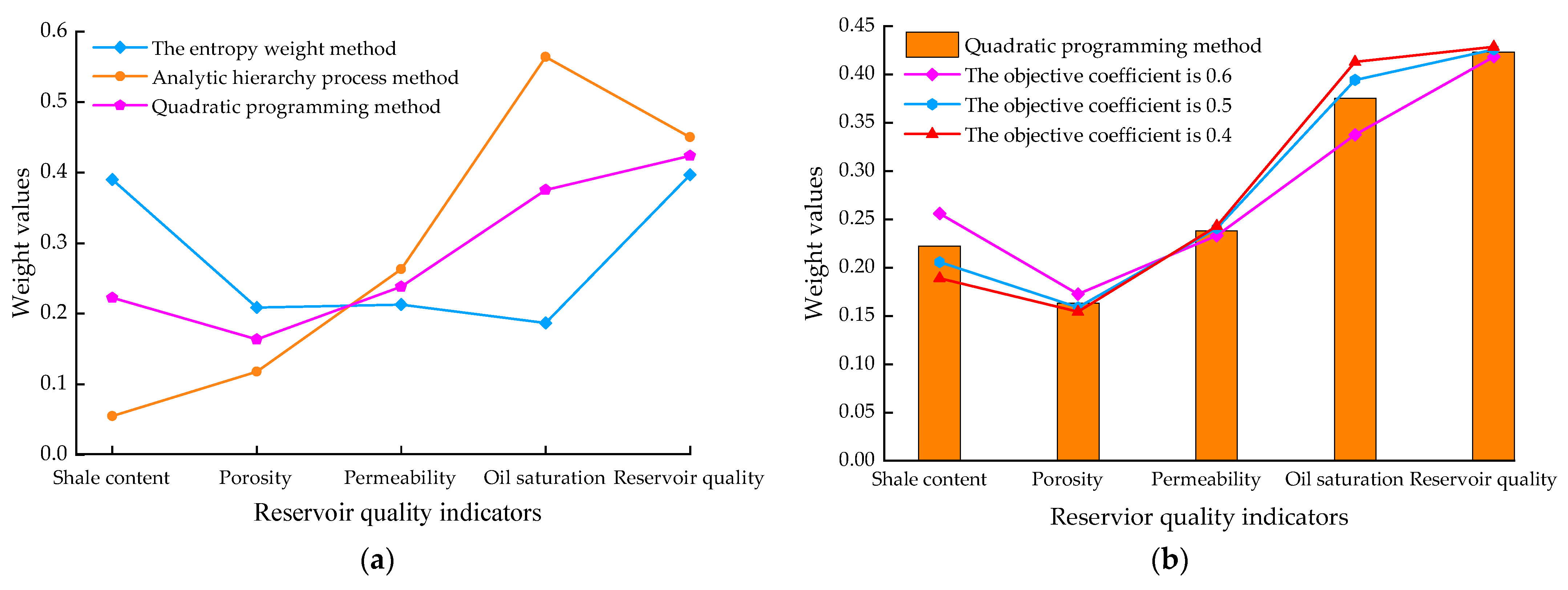
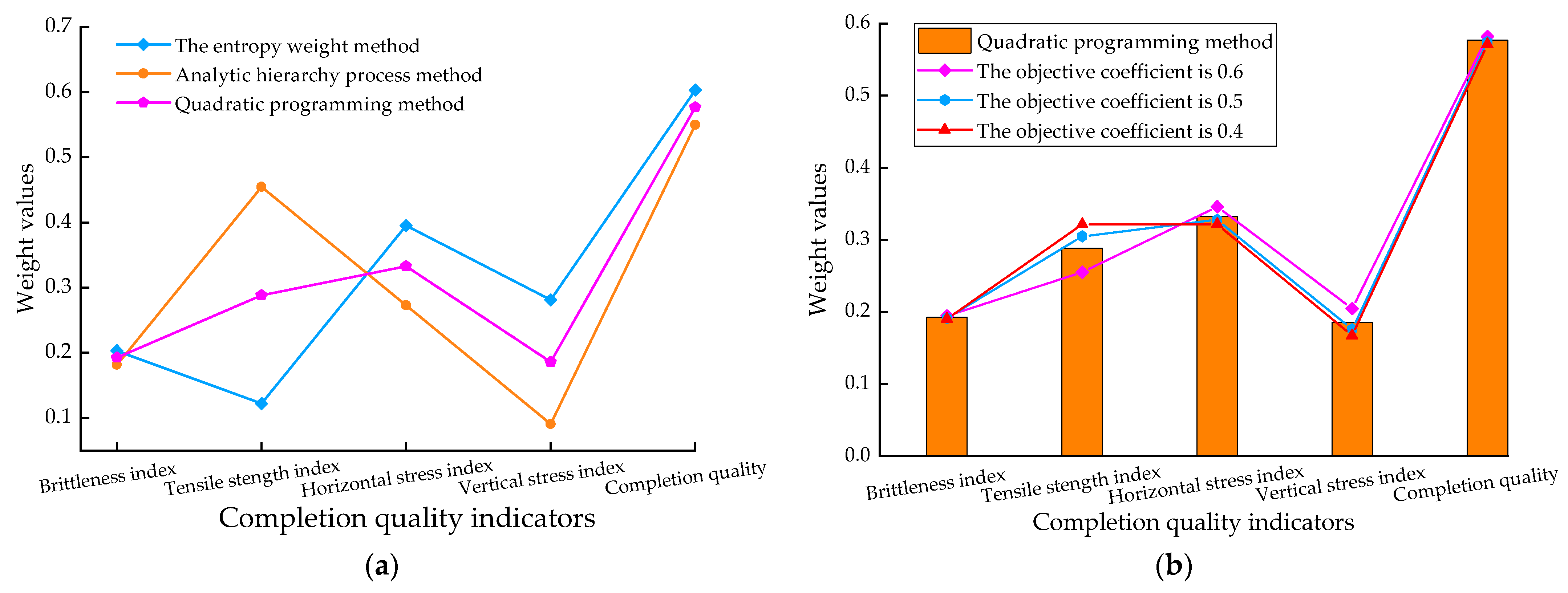
Figure 2a and Figure 3a are the scatter plots of the subjective and objective weighting method and the quadratic combined weighting method for evaluating the three quality indexes, respectively. It can be seen that the quadratic programming method of optimization theory, as an optimal algorithm for solving nonlinear programming problems, can obtain the optimal solution of the combined weighting deviation function. For the weight evaluation results obtained based on the subjective and objective weighting method, the linear weighted grouping method (the objective coefficients were set as 0.6, 0.5, and 0.4 respectively) and the quadratic programming combined weighting method were used to combine the weights, and the results are shown in Figure 2b and Figure 3b. As can be seen from the figure, the robustness of the linear weighted grouping method is poor, and the weight changes of some evaluation indicator fluctuate greatly with different values of the objective coefficients. This is because it is easy to produce weight preference when a fixed value is used to roughly represent the importance of a certain weighting method, so that the importance of some evaluation indicators to the comprehensive weight value is artificially enhanced or reduced.
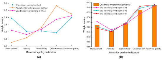
Figure 2.
Weight values of reservoir quality: (a) comparison between EWM, AHP, and quadratic programming; (b) comparison between linear combination weighting and quadratic programming method.
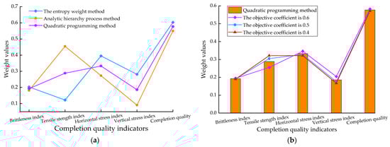
Figure 3.
Weight values of completion quality: (a) comparison between EWM, AHP and quadratic programming; (b) comparison between linear combination weighting and quadratic programming method.
3.2. Determination of Clustering Number Value
The “Silhouette coefficient” is used to evaluate the clustering effect of GMM, so as to determine the clustering number value, which is selected according to the change in the silhouette coefficient with by combining the two factors of cohesion and separation degree. The silhouette coefficient is between −1 and 1, and the closer the distance between the samples in the cluster is, the farther the distance between the samples in the cluster is, the larger the overall silhouette coefficient is, and the better the clustering effect is. Figure 4 is a schematic diagram of determined by the silhouette coefficient method. As the value of increases, the silhouette coefficient increases first and then decreases. When the value is 5, the maximum silhouette coefficient is 0.993, which is the value in the red circle. Therefore, it can be seen that the GMM clustering algorithm is the best to divide the composite quality index into five clustering categories.
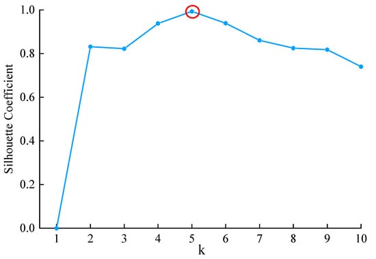
Figure 4.
The value of clustering was determined by the silhouette coefficient method.
3.3. Cluster Simulation Experiment
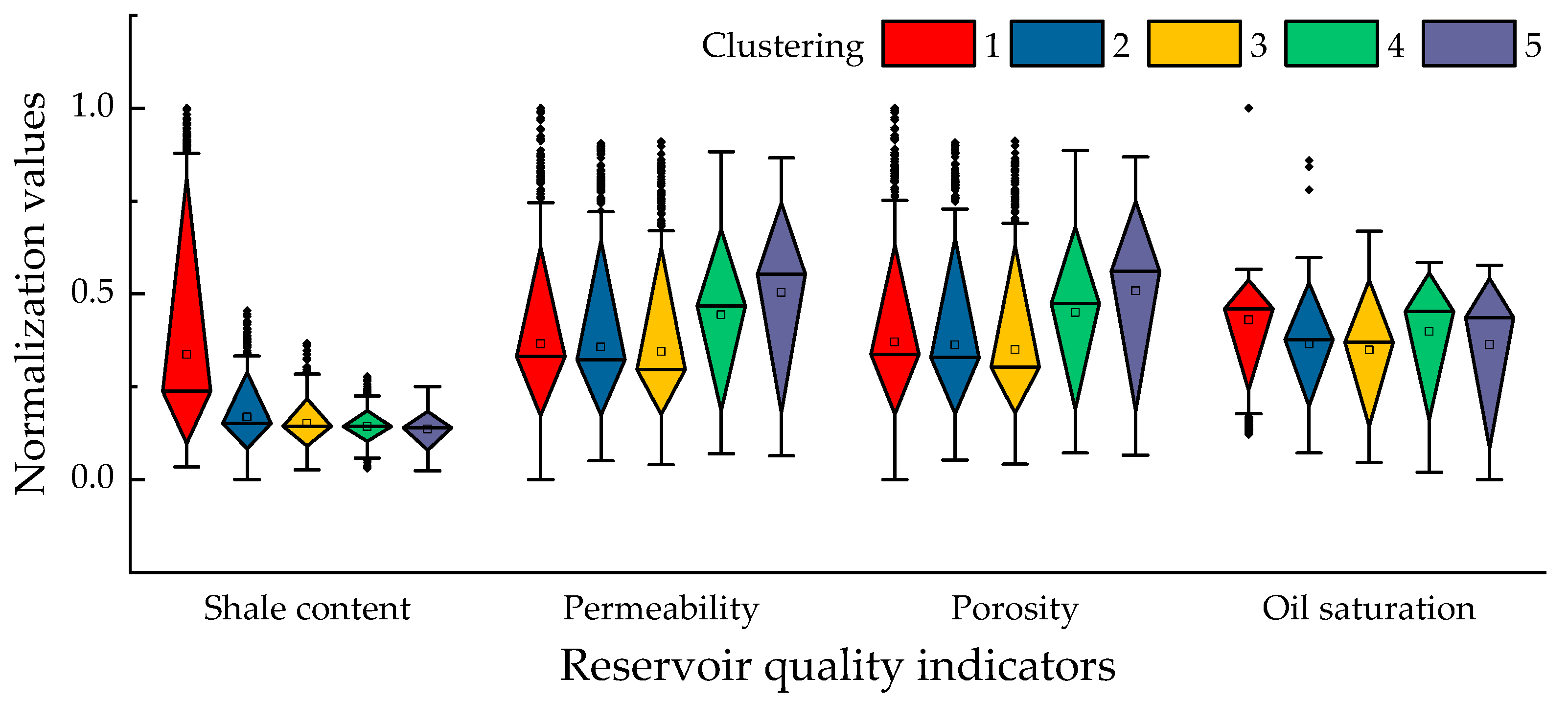
After the standardized treatment of the composite quality index of well A, the training of the GMM clustering model and the classification of the cluster were carried out. Finally, the distribution boxplots of each evaluation indicator that constituted the three quality indexes under different clustering categories were drawn, respectively.
According to the distribution boxplot of the reservoir quality index in Figure 5, category 1 has a high shale content and oil saturation, and relatively low permeability and porosity; that is, the reservoir of Category 1 has the best physical properties. The comparison between Category 2 and Category 3 shows that the differences in shale content, permeability, porosity, and oil saturation are relatively small, indicating that the reservoir quality of Category 1 and Category 2 are similar. In Categories 4 and 5, the shale content is low, but the permeability, porosity, and oil saturation are high, indicating that the reservoir quality is better in Category 4.
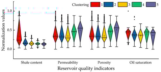
Figure 5.
Boxplot of the reservoir quality evaluation index for well A.
Figure 6 shows the distribution boxplot of the completion quality indicators. It can be seen that Category 1 has a high brittleness index and a low fracture toughness index, horizontal stress difference index, and vertical stress difference index, and the reservoir has a good fracability; that is, the completion quality of Category 1 is the best. A comparison between Categories 2 and 3 shows that there are small differences in the brittleness index, fracture toughness index, horizontal stress difference index, and vertical stress difference index between Category 2 and Category 3, indicating that the completion quality of Category 2 and Category 3 is similar. The comparison between Categories 4 and 5 shows that Category 4 has the lowest brittleness index, but the fracture toughness index and horizontal stress difference index are lower than those of Category 5; so, the completion quality of the Category 4 reservoir is better than that of the Category 5 reservoir.
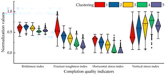
Figure 6.
Boxplot of the completion quality evaluation index for well A.
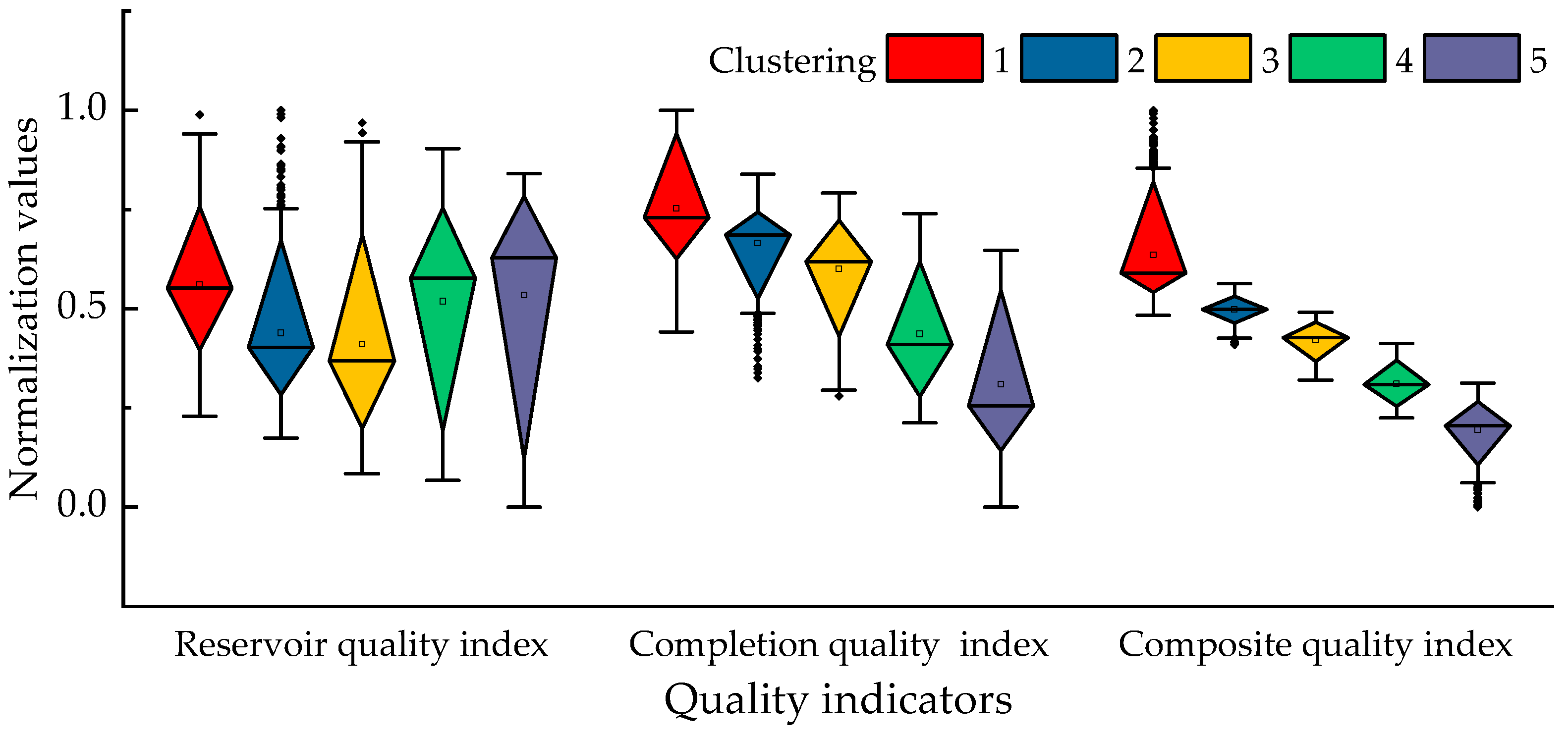
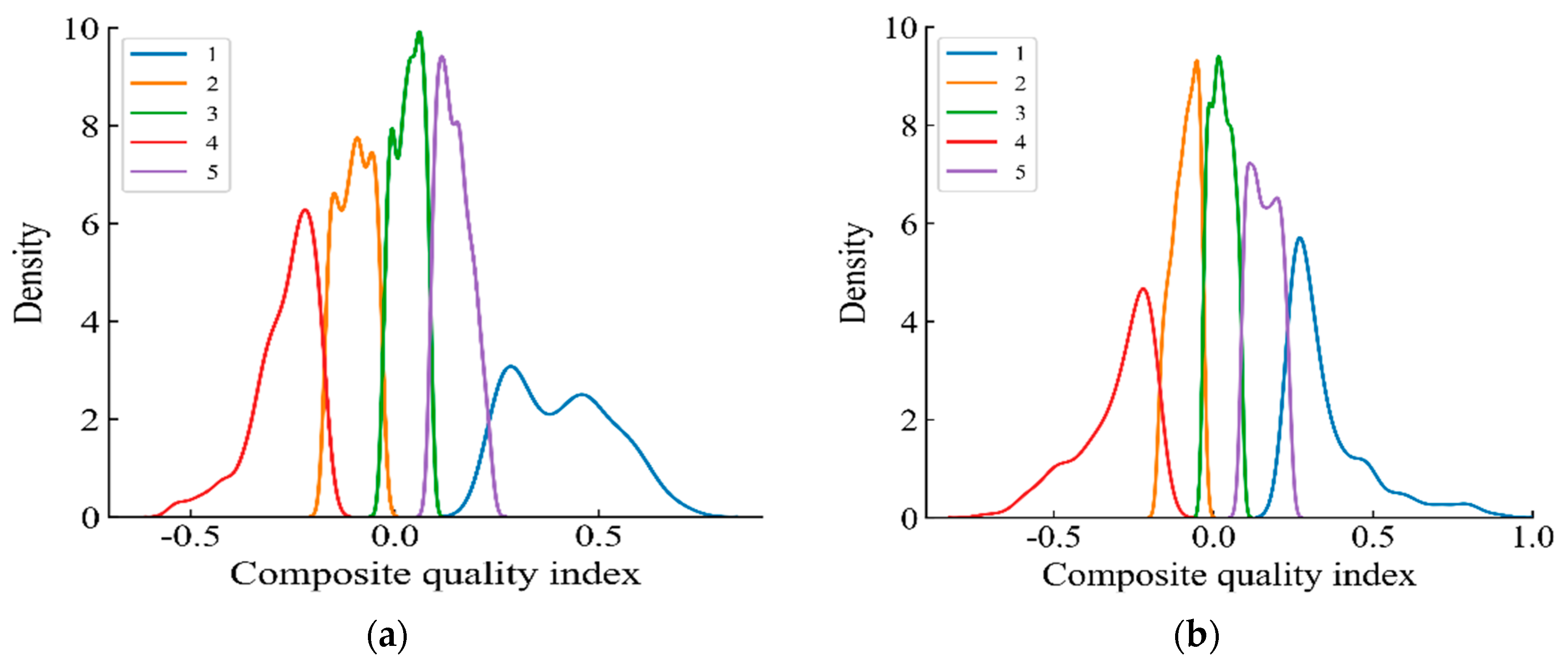
It can be seen from boxplot Figure 7 that the reservoir quality index and completion quality index of Category 1 are high, indicating that the composite quality index of Category 1 is the highest. The quality index differences between Category 2 and Category 3 were minimal by comparative analysis; so, Category 2 and Category 3 were classified into the same category. Compared with Category 4, Category 5 has a lower reservoir quality index, but it has a higher completion quality index and composite quality index. Therefore, the Category 5 reservoir is the least fracability and less prone to fracturing than Category 4. Figure 8a shows the gaussian density distribution of the clustering category of well A, indicating the distribution relationship among the five clustering categories and verifying the accuracy of the GMM clustering model.

Figure 7.
Boxplot of the composite quality evaluation index for well A.
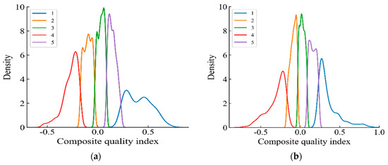
Figure 8.
Gaussian density distribution of the clustering categories: (a) density distribution map of the cluster class in well A; (b) density distribution map of the cluster class in well B.
Comprehensive analysis shows that Category 1 is the Grade 1 of fracturing grades; Categories 2 and 3 are Grade 2; Category 4 and Category 5 are Grade 3 and Grade 4, respectively. Typically, the last two grades are poor quality and can be selected according to the needs of the fracturing operation.
3.4. Cluster Test Experiment
Through the cluster simulation test, well A is clustered into four fracturing grades. Grade 1 and Grade 2 is the preferred fracturing, and Grade 3 and Grade 4 are selected according to the fracturing requirements. The fracturing grade of the cluster are compared with the fracturing stages and oil production of the well.
As shown in Figure 9, the section from 4024.0 to 4472.0 m in well A was divided into two grades, Grade 1 and Grade 4, based on reservoir quality index and completion quality. For reservoir quality (RQ), Grade 1 (blue) indicates the best reservoir properties, Grade 4 (red) indicates the worst reservoir properties, and for completion quality (CQ), Grade 1 (blue) indicates the best reservoir fracability and Grade 4 (red) indicates the worst reservoir fracability. RQ and CQ are weighted into composite reservoir quality (CQI), with Grade 1 (blue) representing the highest fracturing grade, Grade 2 (green) representing the second fracturing grade, Grade 3 (yellow) and Grade 4 representing the third and fourth fracturing grade, respectively, and the fracturing grade is low and not recommended. It can be seen that a fracturing grade with a high reservoir quality index does not necessarily have a high completion quality index. This is because although the evaluation of the reservoir quality is good, the corresponding fracturing effect is poor. Therefore, the comprehensive quality index was selected to classify the well segments. This method not only integrated the physical properties of reservoir quality and the fracability of the completion quality, but also avoided the subjective uncertainty caused by setting thresholds to classify the fracturing stages.
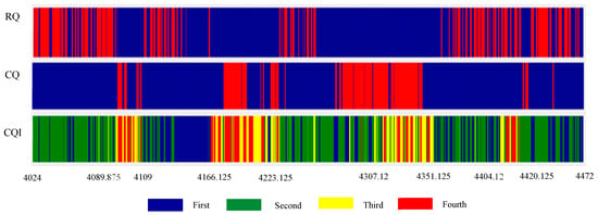
Figure 9.
GMM clustering results of well A.
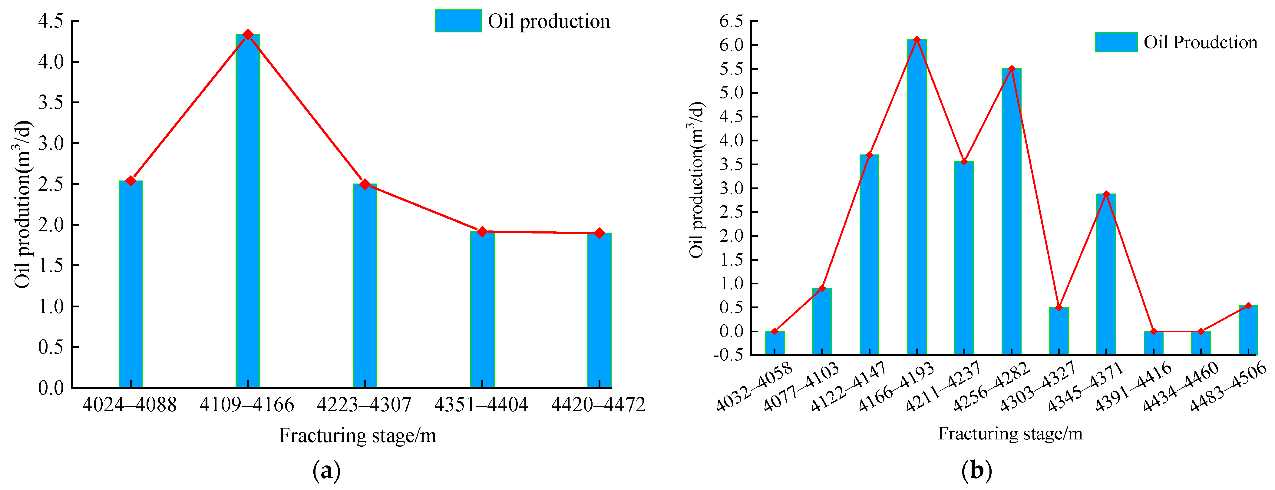
According to the composite quality index, as shown in Table 3, 4109.0–4166.1 m is the first-grade fracturing; 4024.0–4089.9 m, 4223.1–4307.3 m, 4351.2–4404.1 m, and 4420.1–4472.0 m are the second-grade fracturing. The 4307.1–4351.1 m was the third-grade fracturing, and the 4089.9–4109.0 m, 4166.1–4223.1 m and 4404.1–4420.1 m were the fourth-grade fracturing. By comparing the fracturing grades divided by GMM clustering model with the actual fracturing stages and oil production, it can be seen that Grade 1 and Grade 2 are exactly the fracturing grades required by the actual fracturing, while Grade 3 and Grade 4 have low evaluation grades and poor fracturing benefits, and these two grades are not used as the fracturing in the actual construction. The reservoir composite quality index of Grade 1 fracturing is the highest, and the oil production of the fracturing stage is also the highest at 4.331 m3/d after fracturing. Figure 10a shows the daily oil production of each fracturing stage under actual operation. Comprehensive analysis shows that the clustering result of well A is consistent with the actual fracturing stage and oil production, which confirms the rationality of the GMM clustering method selected in this paper.
Table 3.
Comparison of the test and actual fracturing stages in well B.

Figure 10.
Oil production: (a) the oil production of well A; (b) the oil production of well B.
3.5. Cluster Prediction Test
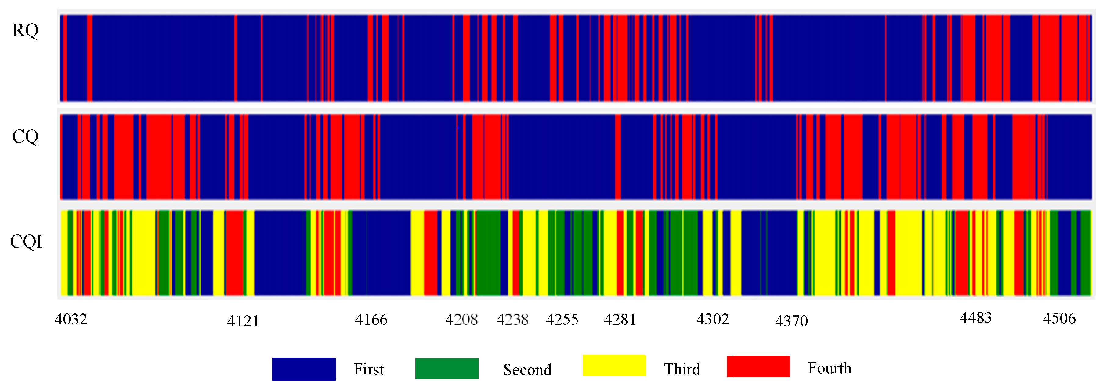
The trained GMM clustering model was used to predict the clustering category of fracturing grades and identify the fracturing grades of the 4032–4506 m reservoir composite quality index in well B, as shown in Figure 11. It can be seen from Figure 11 that the fracturing Grade 1 identified by clustering exactly corresponds to the fracturing stage with high production in actual construction, while Grade 3 and Grade 4 are the stages with no production or no construction in actual construction.
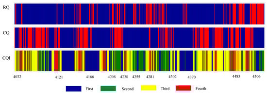
Figure 11.
GMM clustering results of well B.
Table 4 shows the comparison between the fracturing grades predicted by the GMM clustering model and the actual fracturing stages and oil production. It can be seen that the fracturing grades predicted by the clustering model are highly consistent with the actual fracturing stages. The analysis of the predicted results shows that the fracturing grades of 4032.0–4057.0 m, 4389.5–4410.9 m, and 4424.1–4462.5 m predicted by the GMM clustering model are 4, 3, and 4, respectively, and the fracture grades are low and difficult to fracture. However, in the actual fracturing, 4032.0–4058.0 m, 4391.0–4416.0 m, and 4434.0–4460.0 m were used as the fracturing stages. The oil production was 0 after fracturing (the gaussian density distribution of clustering categories and oil production of well B are shown in Figure 8b and Figure 10b, respectively), which indicates that the GMM clustering model can filter out the fracturing grades with low or no production and has good robustness.
Table 4.
Comparison of the prediction and actual fracturing stages in well B.
4. Conclusions
In this paper, the logging data of the natural gamma ray, natural potential, density, and interval transit time are used to excavate various reservoir information, and the reservoir quality, completion quality, and composite quality are considered comprehensively, and the three quality indexes are accurately extracted. According to the logging data of shale oil wells A and B of the Permian Lucaogou Formation in Jimsar Sag, Junggar Basin, the reservoir was evaluated, and the evaluation results were used to classify the clustering categories and identify the fracturing grades. Then, the results of wells A and B were compared with the actual fracturing stage and oil production, and the following conclusions were obtained:
(1) A set of the EWM and AHP coupled evaluation model is established, which comprehensively considers the initiative of the subjective decision-maker and the characteristics of objective data when evaluating reservoir quality, completion quality, and composite quality, and integrates the subjective and objective weights impartially through a constrained nonlinear programming method of optimization theory. The evaluation results show that the coupling evaluation model can reflect the comprehensive quality of the reservoir more effectively and has a certain practical value.
(2) The GMM clustering algorithm is used to classify the reservoir composite quality, which can effectively identify the fracturing grade of the reservoir, and divide the fracturing grade into four grades, namely, I > II > III > IV. The convergence rate of the GMM clustering model is fast, and the efficient EM algorithm is adopted, which has a good clustering effect on the non-spherical data set with the change of well depth.
(3) According to the comparison analysis of the fracturing grades identified by the GMM cluster model with the actual fracturing stages and oil production of wells A and B, it is found that the first fracturing grade has the highest oil production, the second fracturing grade is lower than the first fracturing grade, while the third and fourth fracturing stages have not been constructed or have no oil production The accuracy of the GMM model proposed in this paper is verified, which provides a favorable basis for determining the perforation location of multi-cluster fracturing.
Author Contributions
Conceptualization, L.Y.; Data curation, L.Y.; Funding acquisition, X.W.; Investigation, L.Y., M.F. and Y.Z.; Methodology, Y.Z.; Project administration, Y.Z. and W.W.; Resources, M.F.; Supervision, M.F.; Writing—original draft, W.W.; Writing—review & editing, W.W. All authors have read and agreed to the published version of the manuscript.
Funding
This research was funded by China National Petroleum Corporation grant number 2020B-4118, And The APC was funded by China National Petroleum Corporation.
Institutional Review Board Statement
Not applicable.
Informed Consent Statement
Not applicable.
Data Availability Statement
Not applicable.
Conflicts of Interest
The authors declare no conflict of interest.
References
- Hu, W.; Wei, Y.; Bao, J. Development of the theory and technology for low permeability reservoirs in China. Pet. Explor. Dev. 2018, 45, 646–656. [Google Scholar] [CrossRef]
- Lei, Q.; Guan, B.; Cai, B.; Wang, X.; Xu, Y.; Tong, Z.; Wang, H.; Fu, H.; Liu, Z.; Wang, Z. Technological progress and prospects of reservoir stimulation. Pet. Explor. Dev. 2019, 46, 580–587. [Google Scholar] [CrossRef]
- Li, Q.; Ma, X.; Gao, B.; Chen, X. Progress and Enlightenment of Exploration and Development of Major Shale Oil Zones in the USA. Xinjiang Pet. Geol. 2021, 42, 630–640. [Google Scholar]
- Lei, Q.; Xu, Y.; Cai, B.; Guan, B.; Wang, X.; Bi, G.; Li, H.; Li, S.; Ding, B.; Fu, H.; et al. Progress and prospects of horizontal well fracturing technology for shale oil and gas reservoirs. Pet. Explor. Dev. 2022, 49, 166–172. [Google Scholar] [CrossRef]
- Li, G.; Liu, G.; Hou, Y.; Zhao, X.; Wu, J.; Li, S.; Xian, C.; Liu, H. Optimization method of favorable lithofacies and fracturing parameter for continental shale oil. Acta Pet. Sin. 2021, 42, 1405–1416. [Google Scholar]
- Chen, G.; Bai, Y.; Chen, X.; Xu, B.; Zhu, Y.; Feng, R.; Chen, L. A new identification method for the longitudinal integrated shale oil/gas sweet spot and its quantitative evaluation. Acta Pet. Sin. 2016, 37, 1337–1342. [Google Scholar]
- Miller, C.; Waters, G.; Rylander, E. 2011: Evaluation of Production Log Data from Horizontal Wells Drilledin Organic Shales. In Proceedings of the North American Unconventional Gas Conference and Exhibition, The Woodlands, TX, USA, 14–16 June 2011. [Google Scholar]
- Wigger, E.; Viswanathan, A.; Fisher, K.; Slocombe, R.W.; Kaufman, P.; Chadwick, C. Logging Solutions for Completion Optimization in Unconventional Resource Plays; Society of Petroleum Engineers: Danbury, CT, USA, 2014. [Google Scholar]
- Suarez-Rivera, R.; Deenadayalu, C.; Chertov, M.; Hartanto, R.N.; Gathogo, P.; Kunjir, R. Improving horizontal completions on heterogeneous tight shales. In Proceedings of the Canadian Unconventional Resources Conference, Calgary, AB, Canada, 15–17 November 2011. [Google Scholar]
- Suarez-Rivera, R.; Vaaland Dahl, G.; Borgos, H.; Paddock, D.; Handwerger, D. Seismic-based heterogeneous Earth model improves mapping reservoir quality and completion quality in tight shales. In Proceedings of the Unconventional Resources Conference and Exhibition—USA, The Woodlands, TX, USA, 10–12 April 2013. [Google Scholar]
- Zou, C.; Dong, D.; Wang, Y.; Li, X.; Huang, J.; Wang, S.; Guan, Q.; Zhang, C.; Wang, H.; Liu, H.; et al. Shale gas in China: Characteristics, challenges and prospects (II). Pet. Explor. Dev. 2016, 43, 166–178. [Google Scholar] [CrossRef]
- Lei, Q.; Weng, D.; Xiong, S.; Liu, H.; Guan, B.; Deng, Q.; Yan, X.; Liang, H.; Ma, Z. Progress and development directions of shale oil reservoir stimulation technology of China National Petroleum Corporation. Pet. Explor. Dev. 2021, 48, 1035–1042. [Google Scholar] [CrossRef]
- Liu, G. Challenges and countermeasures of log evaluation in unconventional petroleum exploration. Pet. Explor. Dev. 2021, 48, 891–902. [Google Scholar] [CrossRef]
- Zhang, D.; Yu, Y.; Li, S.; Chen, Y.; Xu, J. Staging optimization of multi-stage perforation fracturing based on unsupervised machine learning. J. China Univ. Pet. 2021, 45, 59–66. [Google Scholar]
- Slocombe, R.; Acock, A.; Fisher, K.; Viswanathan, A.; Chadwick, C.; Reischman, R.; Wigger, E. Eagle Ford Completion Optimization Using Horizontal Log Data. In Proceedings of the SPE Annual Technical Conference and Exhibition, New Orleans, LA, USA, 30 September–2 October 2013. [Google Scholar]
- Cipolla, C.; Weng, X.; Onida, H.; Nadaraja, T.; Ganguly, U.; Malpani, R. New Algorithms and Integrated Workflow for Tight Gas and Shale Completions. In Proceedings of the SPE Annual Technical Conference and Exhibition, Denver, CO, USA, 30 October–2 November 2011. [Google Scholar]
- Atanayev, A.; Nadezhdin, S.; Al Zeidi, O.; Batmaz, T.; Kurniadi, S.D. An Advanced Workflow for Determining Fracture Geometry in Complex Tight Oil Formations in the Sultanate of Oman; Society of Petroleum Engineers: Danbury, CT, USA, 2016. [Google Scholar]
- Cipolla, C.L.; Lewis, R.E.; Maxwell, S.C.; Mack, M.G. Appraising Unconventional Resource Plays: Separating Reservoir Quality from Completion Effectiveness. In Proceedings of the International Petroleum Technology Conference, Bangkok, Thailand, 15–17 November 2011. IPTC 14677. [Google Scholar]
- Ejofodomi, E.A.; Varela, R.A.; Cavazzoli, G.; Velez, E.I.; Peano, J. Development of an Optimized Completion Strategy in the Vaca Muerta Shale with an Anisotropic Geomechanical Model. In Proceedings of the European Unconventional Conference and Exhibition, Vienna, Austria, 25–27 February 2014. [Google Scholar]
- Salah, M.; Ibrahim, M. Engineered Fracture Spacing Staging and Perforation Cluster Spacing Optimization for Multistage Fracturing Horizontal Wells. In Proceedings of the SPE Annual Technical Conference and Exhibition, Dallas, TX, USA, 24–26 September 2018. [Google Scholar]
- Li, H.; Liu, C.; Lu, Y.; Jiang, B.; Du, X. New Method of Tight Oil Horizontal Well Multi-cluster Perforation Design and Its Application. Well Logging Technol. 2018, 42, 362–366. [Google Scholar]
- Xia, H.; Lai, J.; Li, G.; Yang, B. Sweet Spot Prediction of Shale Oil Reservoir Based on Logging Data. J. Southwest Pet. Univ. 2021, 43, 199–207. [Google Scholar]
- Zeng, W. Logging Interpretation Techniques for Determining Permeability. Well Logging Technol. 1979, 3, 1–11. [Google Scholar]
- Li, Q.; Zhou, R.; Zhang, J.; Wu, H.; Li, X. Relations between Archie’s formula and reservoir pore structure. Oil Gas Geol. 2002, 4, 364–367. [Google Scholar]
- Jin, X.; Shah, S.N.; Roegiers, J.C.; Zhang, B. An integrated petrophysics and geomechanics approach for fracability evaluation in shale reservoirs. Soc. Pet. Eng. J. 2015, 20, 518–526. [Google Scholar] [CrossRef]
- Rickman, R.; Mullen, M.J.; Petre, J.E.; Grieser, W.V.; Kundert, D. Apracticaluse of shale petrophysics for stimulation design optimization: All shale plays are not clones of the Barnett Shale. In Proceedings of the SPE Annual Technical Conference and Exhibition, Denver, CO, USA, 21–24 September 2008; Society of Petroleum Engineers: Danbury, CT, USA, 2008. [Google Scholar]
- Li, N.; Zou, Y.; Zhang, S.; Ma, X.; Zhu, X.; Li, S.; Cao, T. Rock brittleness evaluation based on energy dissipation under triaxial compression. J. Pet. Sci. Eng. 2019, 183, 106349. [Google Scholar] [CrossRef]
- Jin, Y.; Chen, M.; Zhang, X. Determination of Fracture Toughness for Deep Well Rock with Geophysical Logging Data. Chin. J. Rock Mech. Eng. 2001, 4, 454–456. [Google Scholar]
- Jin, Y.; Chen, M.; Wang, H.; Ruan, Y. Study on prediction method of fracture toughness of rock mode II by logging data. Chin. J. Rock Mech. Eng. 2008, S2, 3630–3635. [Google Scholar]
- Song, L.; Liu, Z.; Li, C.; Hu, S. Geostress logging evaluation method of tight sandstone based on transversely isotropic model. Acta Pet. Sin. 2015, 36, 707–714. [Google Scholar]
- Yang, Y. Evaluation and analysis of weight assignment method in multi-index comprehensive evaluation. Stat. Decis. 2006, 13, 17–19. [Google Scholar]
- Chuan, Y. Entropy-based weights on decision makers in group decision-making setting with hybrid preference representations. Appl. Soft Comput. 2017, 60, 737–749. [Google Scholar]
- Deng, X.; Li, J.; Zeng, H. Research on Computation Methods of AHP Wight Vector and Its Applications. Math. Pract. Theory 2012, 42, 93–100. [Google Scholar]
- Mai, T.; Mortari, D. Theory of functional connections applied to quadratic and nonlinear programming under equality constraints. J. Comput. Appl. Math. 2021, 406, 113912. [Google Scholar] [CrossRef]
- Huang, Z.; Xiang, Y.; Zhang, B.; Wang, D.; Liu, X. An Efficient Method for K-Means Clustering. Pattern Recognit. Artif. Intell. 2010, 23, 516–521. [Google Scholar]
- Lloyd, S. Least squares quantization in PCM. IEEE Trans. Inf. Theory 1982, 28, 129–137. [Google Scholar] [CrossRef] [Green Version]
- Weber, C.M.; Ray, D.; Valverde, A. Gaussian mixture model clustering algorithms for the analysis of high precision mass measurements. Nucl. Instrum. Methods Phys. Res. Sect. A Accel. Spectrometers Detect. Assoc. Equip. 2022, 1027, 166299. [Google Scholar] [CrossRef]
- Patel, E.; Kushwaha, D.S. Clustering Cloud Workloads: K-Means vs Gaussian Mixture Model. Procedia Comput. Sci. 2020, 171, 158–167. [Google Scholar] [CrossRef]
- Zhang, B.; Shin, Y.C. An Adaptive Gaussian Mixture Method for Nonlinear Uncertainty Propagation in Neural Networks. Neurocomputing 2021, 458, 170–183. [Google Scholar] [CrossRef]


Publisher’s Note: MDPI stays neutral with regard to jurisdictional claims in published maps and institutional affiliations. |
© 2022 by the authors. Licensee MDPI, Basel, Switzerland. This article is an open access article distributed under the terms and conditions of the Creative Commons Attribution (CC BY) license (https://creativecommons.org/licenses/by/4.0/).