Solutions of Feature and Hyperparameter Model Selection in the Intelligent Manufacturing

Abstract

In the era of Industry 4.0, numerous AI technologies have been widely applied. However, implementation of the AI technology requires observation, analysis, and pre-processing of the obtained data, which takes up 60–90% of total time after data collection. Next, sensors and features are selected. Finally, the AI algorithms are used for clustering or classification. Despite the completion of data pre-processing, the subsequent feature selection and hyperparameter tuning in the AI model affect the sensitivity, accuracy, and robustness of the system. In this study, two novel approaches of sensor and feature selecting system, and hyperparameter tuning mechanisms are proposed. In the sensor and feature selecting system, the Shapley Additive ExPlanations model is used to calculate the contribution of individual features or sensors and to make the black-box AI model transparent, whereas, in the hyperparameter tuning mechanism, Hyperopt is used for tuning to improve model performance. Implementation of these two new systems is expected to reduce the problems in the processes of selection of the most sensitive features in the pre-processing stage, and tuning of hyperparameters, which are the most frequently occurring problems. Meanwhile, these methods are also applicable to the field of tool wear monitoring systems in intelligent manufacturing.

1. Introduction

In the recent decades, owing to the development of AI technology, intelligent manufacturing technology has rapidly evolved, including automation, digitization, and intelligence, however, many challenges remain to be overcome. These include the collection of in-line manufacturing data in industry, the long-time consuming in pre-processing, the selection of sensors, features, and AI models, and the tuning of hyperparameters.

A Tool Condition Monitoring (TCM) system has been performed using advanced sensors and computational intelligence to predict and avoid adverse conditions for cutting tools and machinery [1,2,3,4,5,6,7,8,9,10,11,12,13]. The sensors are indispensable parts of intelligent manufacturing. First, the signals of sensors are obtained; second, after a series of data processing techniques, the desired data can be obtained; finally, the obtained data can be input into the AI model to classify or cluster the target topic. However, selection of the suitable sensors is crucial. There are many sensors in the world, including accelerometers, microphones, thermocouples, proximity sensors, acoustic emission sensors, pressure sensors, gas sensors, and position sensors. Use of an excessive number of sensors can increase cost and decrease the performance of the system, whereas using a few important sensors on the tool machine can increase their contribution by adopting features, reducing the cost incurred during sensor installation, model computing, and research. In addition, it would improve the robustness and performance of the system. However, this is a chicken-and-egg conundrum; that is, it is not feasible to clearly judge the suitability of the sensors before installation. Except for the domain knowledge required, the selection of sensors is usually done by sensitivity analysis after acquiring the relevant data, and even the selection of time-domain or frequency-domain features in the sensors. Over the past few decades, statistical methods including Pearson, Spearman, and ANOVA (analysis of variance) correlation coefficient analyses have been commonly used. Moreover, the algorithms in tree family, namely the decision tree, isolation forest, gradient boosting decision tree, and the light gradient boosting machine, have recently been used to compute the feature contribution of data. However, finding the importance of each feature in a neural network model, which is commonly known as a black box, poses a considerable problem. Fortunately, a technique known as Shapley Additive ExPlanations (SHAP) has been proposed to overcome this challenge [14]. The solid theoretical foundation of SHAP can explain any models from tree or neural networks, irrespective of whether the learning model is shallow or deep learning. Therefore, in this study, we compared two traditional analysis methods with SHAP to determine the importance of the features of five different sensors. With the AI models explained, the suitable sensor for reduction of the above cost and improvement of the performance of the system can be determined. The traditional Shapley value has been used for feature selection as early as 2005 [15] and for sensor selection in 2009 [16], but it has not been applied to the field of wear prediction. Until SHAP was invented, some scholars, such as Wang [16], applied SHAP to elucidate the contribution of each feature in the model, except for the intelligent manufacturing domain.

The sensor systems used for monitoring tool wear condition are dynamometers, accelerometers, acoustic emission sensors, current and power sensors, image sensors, and other sensors. Using the processed data obtained from the sensor, the following algorithms are among the most referred methods of deep learning in recent years: Deep multilayer perceptron (DMLP), long-short-term memory (LSTM), convolutional neural network (CNN), and deep reinforcement learning (DRL) [17].

Weili [18] in 2020 designed a nonlinear regression model to predict tool wear based on a new input vector. This method is validated on both NASA Ames milling data set and the 2010 PHM Data Challenge data set. Results show the outstanding performance of the hybrid information model in tool wear prediction, especially when the experiments are conducted under various operating conditions.

However, Serin used a genetic algorithm for feature selection, which is a type of optimization algorithm that requires various parameters for tuning, and Weili used empirical rules for feature extraction. Furthermore, neither Serin nor Weili focused on the hyperparameter tuning of the model. It is important to understand that AI modeling must adhere to the garbage in garbage out principle. Both the feature selection and the hyperparameters of the model will affect the final model performance. In this study, we propose solutions for these two cases.

The current problem is that if a new problem domain is applied with machine learning and deep learning, we have to consider what kind of framework to use at first. After all, deep learning is very sensitive to many different hyperparameters, such as optimizers. The choice of algorithm may even require setting 20 to 50 parameter settings to train a model system with good performance.

Moreover, in addition to the abovementioned feature selection problem, the tuning of hyperparameters is another topic of significance. AutoML seeks to automatically compose and parametrize machine learning algorithms to maximize a given metric, such as predictive accuracy [19,20,21,22,23,24]. The available algorithms are typically related either to preprocessing (feature selection, transformation, imputation, etc.) or to the core functionality (classification, regression, ranking, etc.)

In the past, empirical rules have been used to improve the robustness of the models by gradually adjusting the hyperparameters with experienced AI modeling researchers to reduce the occurrence of underfitting and overfitting. Later on, optimization methods such as Simulated Annealing, Particle Swarm Optimization, and Genetic Algorithm were gradually used for the field of Hyperparameter Optimization (HPO), until 2011, when scholars such as James Bergstra [25] successfully applied the Bayesian optimization method for treed Parzen estimators to achieve a bright performance, followed by Frank Hutter [26] in 2011, and Kevin Swersky [27] in 2013 for searching kernel functions.

In this study, the new cloud-based TCM system is established by using the LSTM model for non-indirect milling cutter monitoring, and the service will eventually propose a recommended optimized hyperparameter and show the improvement in the model performance. In the newly proposed cloud services, users could operate with an interactive and visualized cloud service user interface to tune hyperparameters via a web browser, and the AI model optimization process will be carried out fully automatically by integrating container management and Kubernetes in high-speed computers.

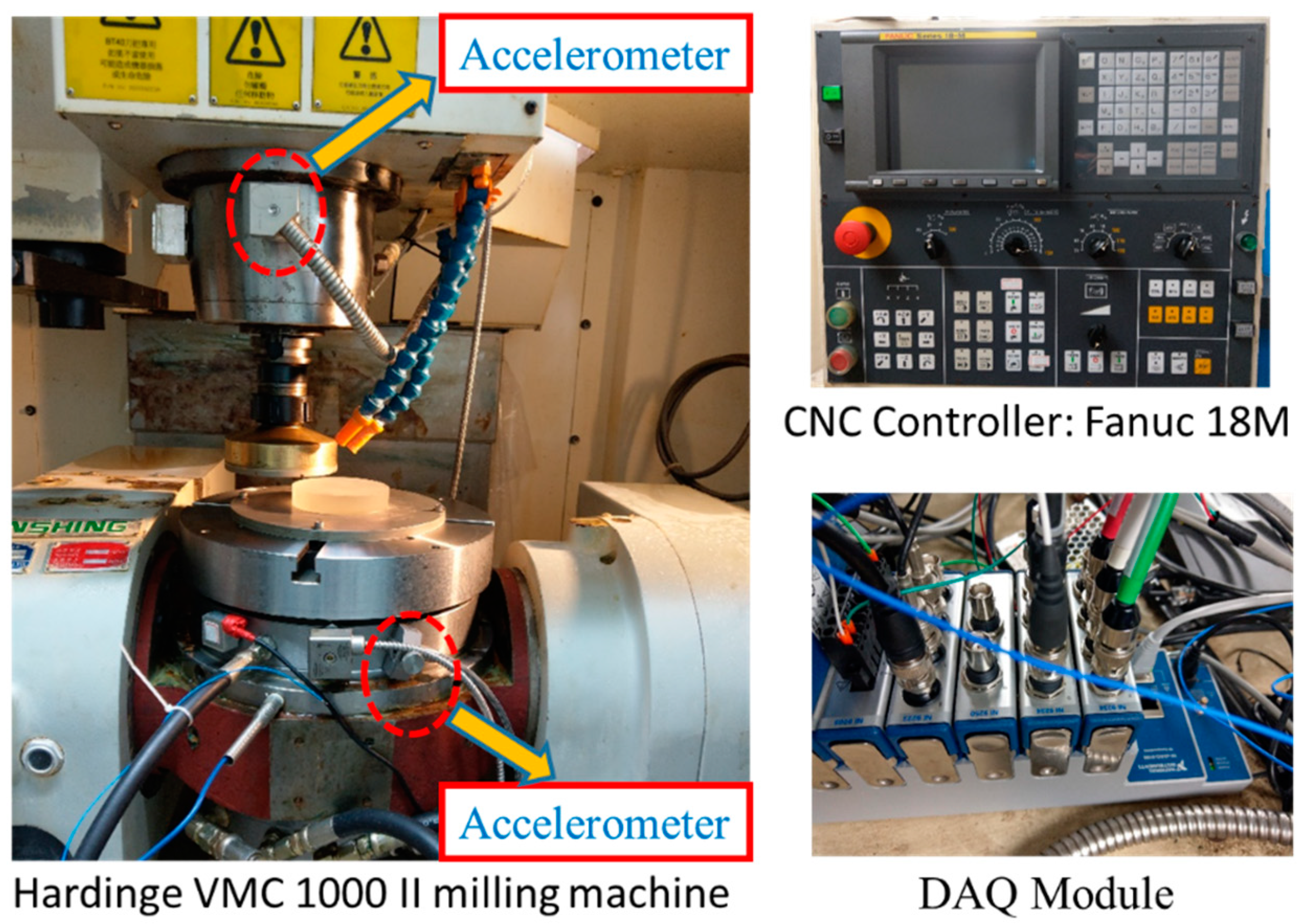
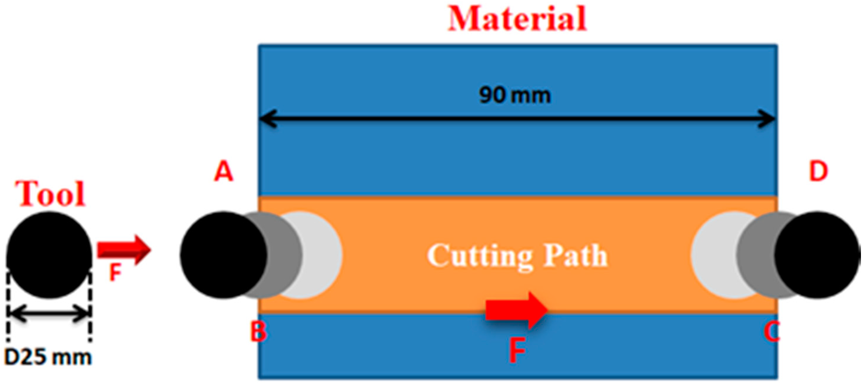
2. Experimental Setup

In this study, an experiment was conducted to analyze the contribution of five different sensors in an intelligent milling machine. As illustrated in Figure 1, the experimental setup consisted of two accelerometers, one condense microphone (not visible in the figure), and one thermocouple installed on the rotating table of a Hardinge VMC 1000 II milling machine; simultaneously, the spindle load was acquired by the NI’s data acquisition module. Since a hydrostatic worktable was installed on the milling machine, the temperature of oil in the worktable was also considered.

The experiment was performed using a Hardinge computer numerical control (CNC) milling machine. The workpiece material was SUS 304 stainless steel, and a JSK 4 tooth carbide end mill milling cutter of straight-line slot milling type was used. The workpiece was processed until each cutter was rendered unusable, and the wear and tear of the tools along with the signals of the five sensors were recorded. The suitability of the sensors was examined based on the assumption that a tool condition monitoring system would be developed using this intelligent tool machine.

To increase the variance of the system, four commonly used cutting parameters were used in the manufacturing processes.

Table 1. Experimental Cutting Parameters.

Tool Number	Spindle Speed (rpm)	Feed Rate (mm/min)	Depth (mm)	Number of Path
1	800	40	0.3	33
2	600	20	0.3	20
3	400	20	0.3	35
4	800	20	0.3	75

provides the experimental conditions of each tool order before the cutter was rendered unusable; namely, spindle speed, feed rate, cutting depth, and milling times. Moreover, each cut was recorded with Charge Coupled Device (CCD) photos and the real wear was calculated. We obtained 22, 30, 35, and 75 data points from each cutting condition. The information of specifications and installation location of the sensors is shown in

Table 2. Sensor Information.

Sensor	Frequency Range	Install Location
Accelerometer	0–8 kHz	Spindle
Accelerometer	0–8 kHz	Worktable
Condense Microphone	0–20 kHz	Spindle
Thermocouple	1 Hz	Worktable
Spindle load	24 Hz	-

, and the milling path is shown in Figure 2.

In the full groove milling workpiece, the tool just entering the workpiece generated unstable signal; in the feed rate and path calculation, milling A is the near tool contact point and D is the exit point; a 10 s signal window is set to capture the stable signal during milling, as shown in Figure 3. The total sensor and the effective feature index of each direction are obtained using wavelet conversion, RMS, SE, Kurtosis, Skewness, and inverse spectrum.

3. Sensors and Features Selection System

In this section, we introduce the selection techniques used in the past and the selection techniques proposed in this study by implementing the SHAP algorithm.

3.1. Methodology

In this study, two traditional correlation coefficient methods, namely the Pearson (linear) correlation and the Spearman (nonlinear) correlation, along with a method to explain the individual predictions of models, namely Shapley Additive ExPlanations (SHAP) method, were applied to calculate the contribution of the features of each sensor.

We acquired a total of 162 data points using the five sensors in the milling machine, as shown in Table 1, and transformed them into a frequency domain using the Fourier fast transform (FFT). Thereafter, the algorithms provided the respective contributions of the signals in the system from the frequency domain.

3.1.1. Correlation Coefficient

Pearson’s correlation coefficient r is a statistical variable used to evaluate the linear correlation between two datasets, whereas Spearman’s rank correlation coefficient ρ is a similar statistical variable for evaluating the nonlinear correlation between two datasets.

To rephrase, Pearson’s correlation r is the covariance of the two variables divided by the product of their standard deviations, and it is expressed as

$$r_{xy}=\frac{{{\displaystyle \sum }}_{i=1}^n\left(x_i-\overline{x}\right)\left(y_i-\overline{y}\right)}{\sqrt{{{\displaystyle \sum }}_{i=1}^n{\left(x_i-\overline{x}\right)}^2}\sqrt{{{\displaystyle \sum }}_{i=1}^n{\left(y_i-\overline{y}\right)}^2}} ,$$

(1)

where $n$ is the sample size; $x_i \mathrm{and} y_i$ are the individual sample points; $\overline{x}=\frac{1}{n}{\displaystyle \sum }_{i=1}^n{x}_i$; and $\overline{y}$ is analogous to $\overline{x}$.

Spearman’s correlation ρ is defined as the Pearson correlation coefficient between the rank variables and can be expressed as

$${\rho }_{xy}=\frac{{{\displaystyle \sum }}_i\left(x_i-\overline{x}\right)\left(y_i-\overline{y}\right)}{\sqrt{{{\displaystyle \sum }}_i{\left(x_i-\overline{x}\right)}^2}\sqrt{{{\displaystyle \sum }}_i{\left(y_i-\overline{y}\right)}^2}} ,$$

(2)

where $x_i \mathrm{and} y_i$ are the individual ranks data; and $\overline{x}$ and $\overline{y}$ are the means of $x$ and $y$, respectively.

Depending on whether the correlation r or ρ is greater than 0.7, between 0.7 and 0.4, or less than 0.4, it is considered as highly correlated, moderately correlated, or modestly correlated, respectively. In general, highly or moderately correlated features are significantly more favorable than modestly correlated features.

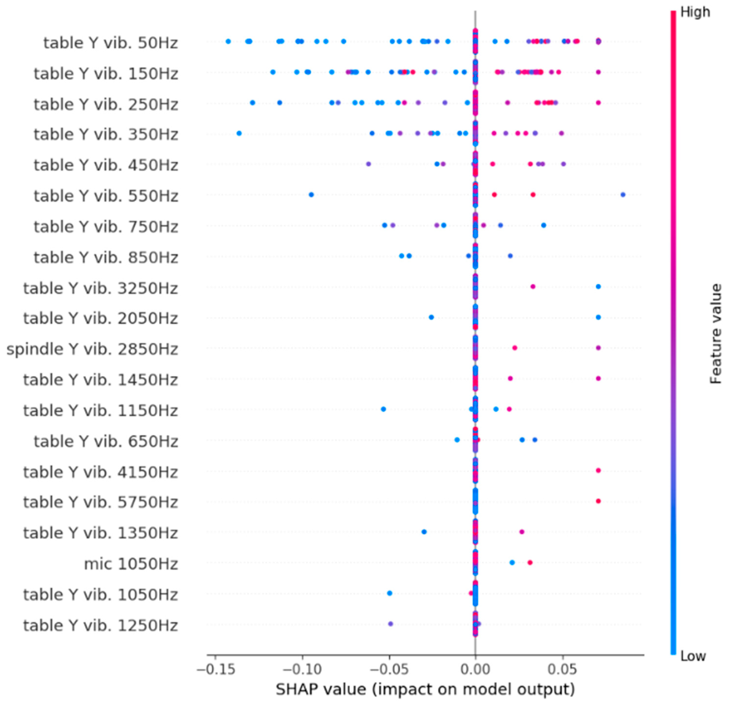
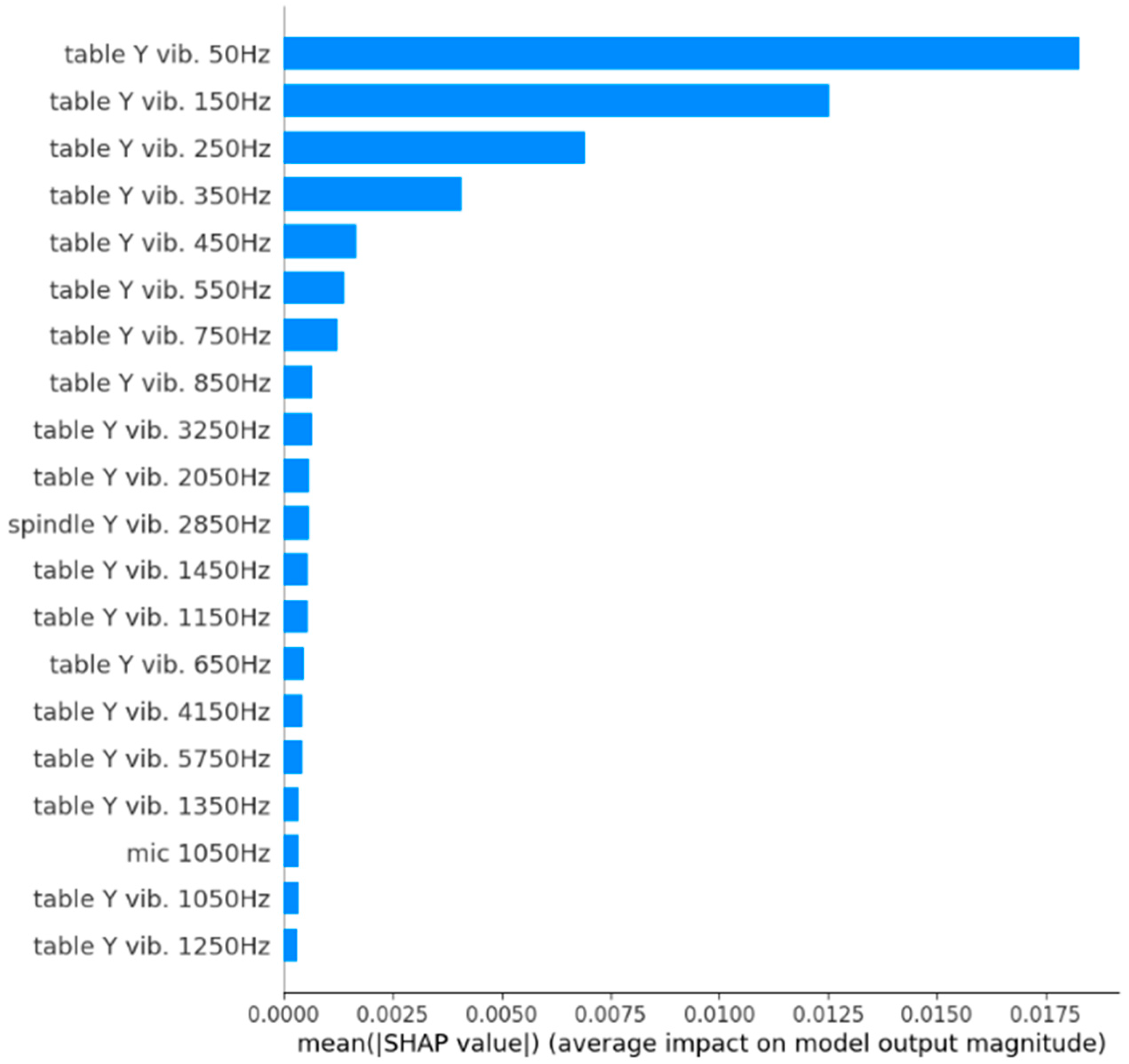
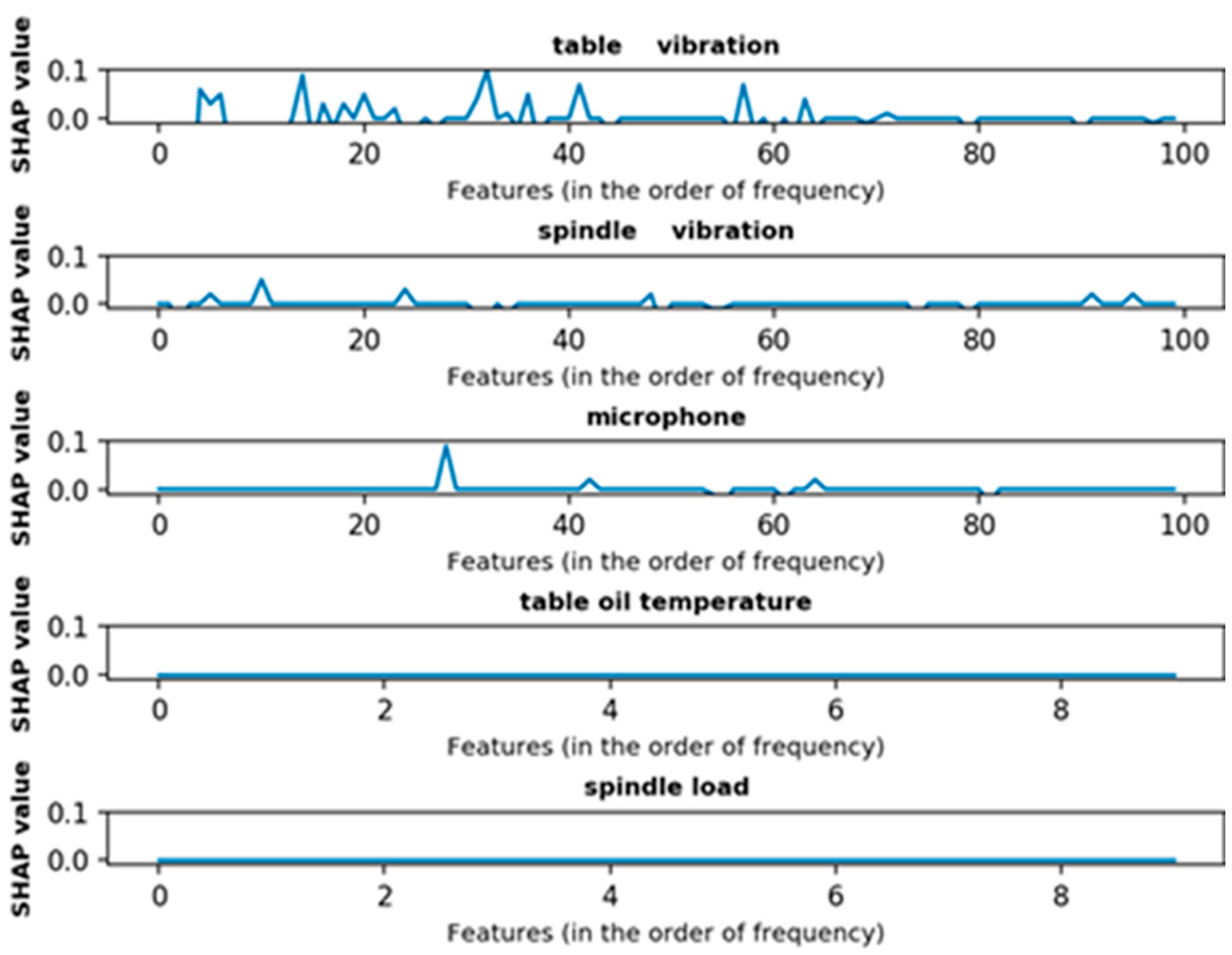
3.1.2. Shapley Additive ExPlanations (SHAP)

SHAP, which was proposed by Lundberg and Lee [14], is a method used to explain the individual predictions of AI models. SHAP is based on the theoretically optimal game Shapley values. Therefore, it is assumed that $n$ is the sample size,$m$ is the feature size, $x_i$ is the individual sample points indexed with $i$, and $x_{i,j}$ is the individual feature indexed with $j$. Therefore, when the prediction value and the base line of this model are $y_i$ and $y_{base}$, respectively, the SHAP value $f\left(x\right)$ will be in accordance with the formula below:

$$y_i=y_{base}+f\left(x_{i,1}\right)+f\left(x_{i,2}\right)+\dots +f\left(x_{i,k}\right) ,$$

(3)

As a result, if the SHAP value $f\left(x_{i,j}\right)>0$, the feature has a positive impact on the prediction value of the system. In contrast, if the SHAP value $f\left(x_{i,j}\right)<0$, the feature would have a negative impact on the system, thus decreasing the performance and robustness of the system. Therefore, the SHAP method can determine the efficient and invalid features as well as obtain information regarding the harmful features.

3.2. Results

To evaluate the contribution of the correlation coefficient methods, the FFT data were divided into bandwidths of 0.1 Hz. As such, the number of features can be improved to improve the system robustness.

Table 3. Feature number of analysis results of Pearson and Spearman correlation coefficient.

Sensor	Highly Correlated r > 0.7	Moderately Correlated 0.7 > r > 0.4	Highly Correlated ρ > 0.7
Accelerometer on worktable	1651	1703	0
Accelerometer on spindle	12,544	32,549	1002
Condense microphone	1380	1075	0
Thermocouple	1	0	0
Spindle load	1	0	0

presents the analysis results of the Pearson and Spearman correlation coefficients, denoted by r and ρ, respectively. As per the table, the accelerometer on the spindle offers the highest contribution (much larger than others) in this tool condition monitoring system, followed by the accelerometer on the worktable and the microphone, whereas the thermocouple and spindle load signals have a negligible impact on the system.

Owing to the high calculation time cost of the SHAP algorithm, the FFT data were divided based on a bandwidth of 100 Hz in the vibration and sound signals and a bandwidth of 4 Hz in the thermocouple and spindle load signals. Figure 4 illustrates the SHAP sum values of each feature for each signal. The vibration signal on the worktable had the largest number of peaks approaching the 0.1 SHAP value; therefore, it was the most sensitive to this system. In addition, the vibration signal and sound also comprised a few peaks; therefore, these two signals had some impact in the system, even though they did not have a discernible vibration signal on the worktable. Moreover, the thermocouple and spindle load signals had an analysis result of zero SHAP value, signifying no impact in this system.

After calculating the SHAP value of each signal, the feature importance scatter and bar plots were constructed. These figures help us understand the details of the intuitive relationship between the features and SHAP values. Based on the results illustrated in Figure 5 and Figure 6, the features of the worktable vibration signals below 1000 Hz had the highest impact on this system. In addition, the spindle vibration signal at 2850 Hz and sound at 1050 Hz had a significant impact. However, if there is a rich variance in these high-impact features, they may not have a positive influence on the system.

As demonstrated in

Table 4. Table of SHAP sum value with largest and smallest 15 items.

Features		Largest SHAP Value	Features		Smallest SHAP Value
table	3250 Hz	0.1	table	150 Hz	−0.56
table	1450 Hz	0.09	table	250 Hz	−0.46
spindle	2850 Hz	0.09	table	350 Hz	−0.26
table	4150 Hz	0.07	table	50 Hz	−0.24
table	5750 Hz	0.07	table	750 Hz	−0.08
table	450 Hz	0.06	table	850 Hz	−0.06
table	650 Hz	0.05	table	1050 Hz	−0.05
table	2050 Hz	0.05	table	1250 Hz	−0.05
table	3650 Hz	0.05	table	1550 Hz	−0.05
mic	1050 Hz	0.05	table	3750 Hz	−0.05
table	3150 Hz	0.04	mic	250 Hz	−0.05
table	6350 Hz	0.04	mic	4950 Hz	−0.05
table	550 Hz	0.03	table	2450 Hz	−0.04
table	1650 Hz	0.03	table	6050 Hz	−0.04

, we determined the largest and smallest items of the SHAP sum value. As per the table, the worktable vibration signals below 1000 Hz were found to have the smallest negative SHAP value, which could lower the performance of this system. Based on the largest SHAP values and their indices, the spindle vibration signals at 2850 Hz and sound at 1050 Hz attained the third and tenth place, respectively, in terms of impact on the system.

4. Hyperparameters Optimization with Tree-Structured Parzen Estimator (TPE)

In this chapter, we will introduce our proposed online cloud service system of automated HPO that integrates the NNI module of Microsoft and the TPE resources.

4.1. Methodology

Methodology includes TPE and interactive cloud service integration. In Bayesian optimization (BO), we can obtain a posteriori probabilistic description of the objective function and, thus, obtain the expected mean and variance of each hyperparameter at each point using the Gaussian process regression. The mean value represents the final desired effect at this point (exploiting); moreover, the larger the mean value, the-larger the indicated final desired value of the model. The variance indicates the uncertainty of the effect at this point (exploration), and the larger the variance, the higher the indicated exploration value at this point.

Based on the BO theorem mentioned above, the Gaussian mixing model and the concept of Parzen tree structure, the Hyperopt, are introduced to form the TPE algorithm, which increases its performance in high-dimensional space compared to the BO algorithm.

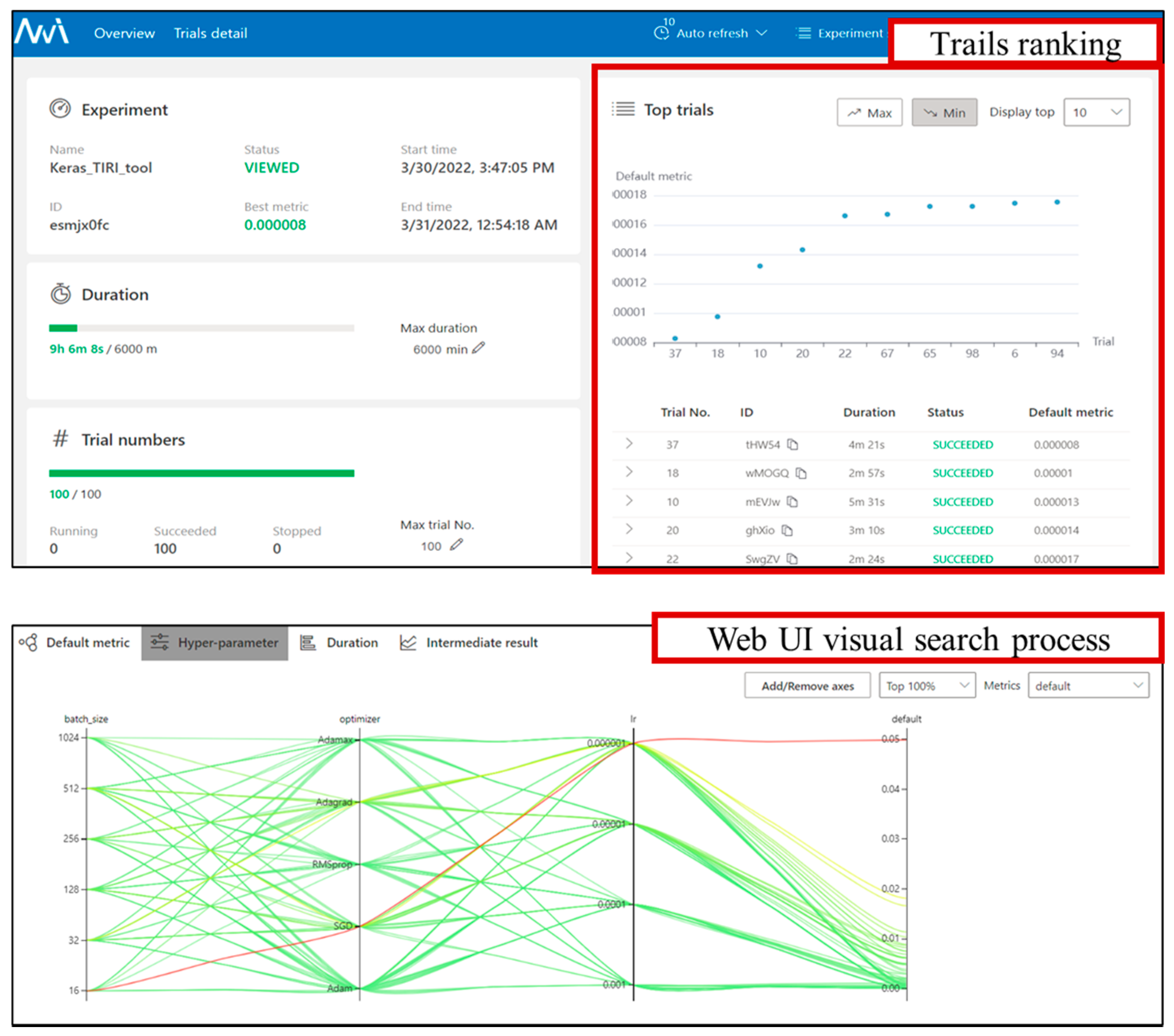
4.2. Cloud Service of Automated HPO

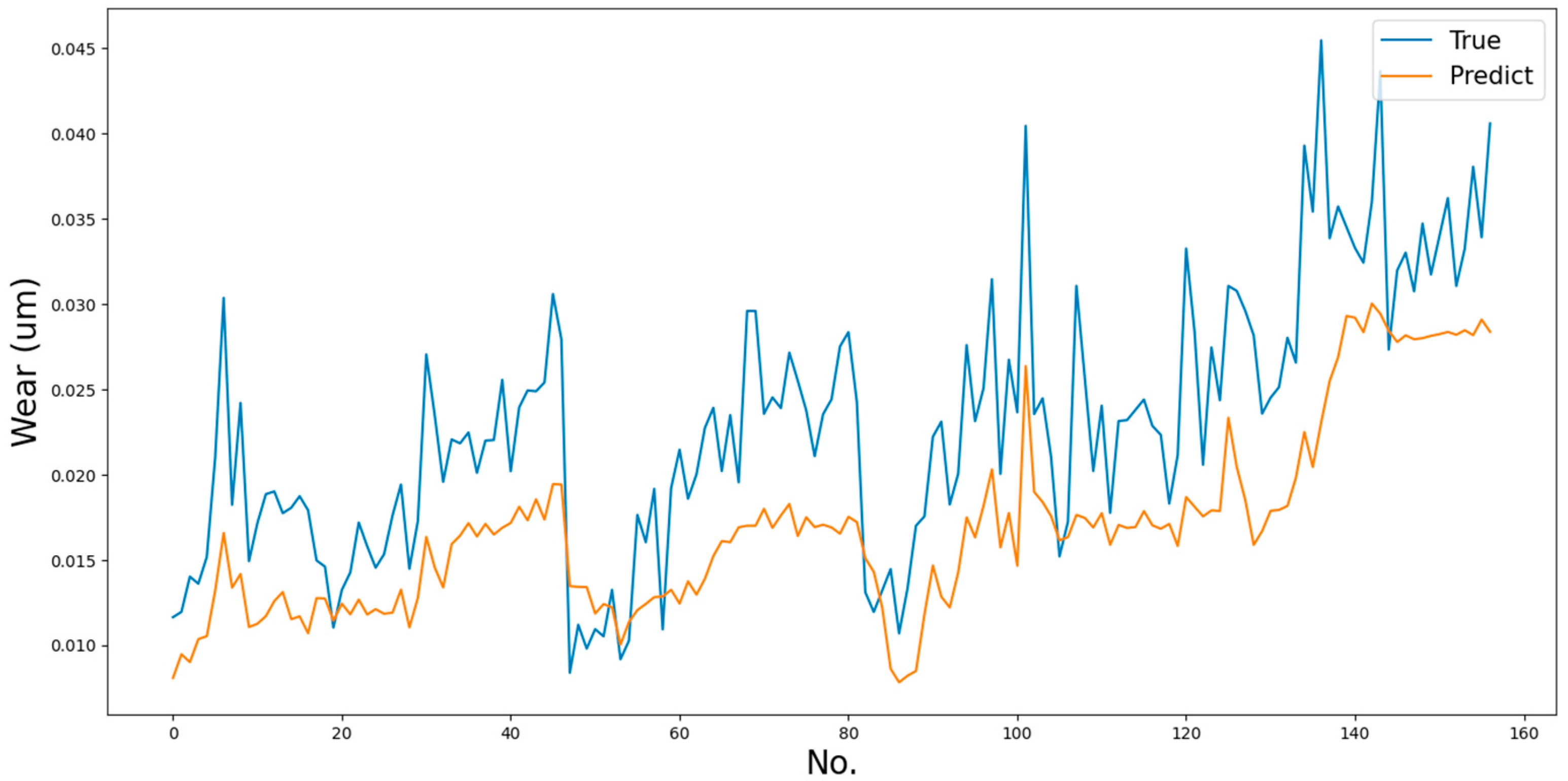
Due to the convenience of grid search and random search algorithms, these are currently the most widely used hyperparametric optimization strategies that can be used in different domains: the number of hidden layers, number of neurons, type of activation function, different learning rates, and batch size. In this study, we first use the milling data of Condition 2, with the sensor signal as input and the CCD image to calculate the wear as the curve output. At first, the LSTM model is trained for hyperparameter tuning and the model architecture is uploaded to the cloud. During the tuning process, Neural Network Intelligence (NNI) [8] provides a friendly visual web interface to monitor the tuning process, and the hyperparameter ranking can be done according to the performance metrics of the model of interest to the user or the algorithm developed by the user. The optimized model can be downloaded, and the interface is shown in Figure 7.

The Light Gradient Boosting Machine (LightGBM) algorithm [27,28,29] performs automatic feature filtering. Based on the histogram algorithm, the training data is traversed, the number of discrete values of each feature is counted, and the corresponding regression curves of the features in the data are ranked according to their mean values.

A Tree-structured Parzen Estimator (TPE) [30] is a sequential model-based optimization method, which is based on the previous model, setting the target hyperparameters to be optimized, establishing a hyperparameter exploration space grid, and then using loss minimization as a criterion for optimization. The hyperparameters are the key factors that affect iterative learning in machine learning, and their settings have a great impact on the training of the model, which is the most pestilent challenge. The purpose of adjusting the hyperparameter exploration is to maintain the model performance and accelerate the speed of model training.

Table 5. Search space settings.

No.	Batch Size	Optimizer	Learning Rate
1	16	Adam	0.001
2	32	SGD	0.0001
3	128	RMSprop	0.00001
4	256	Adagrad	0.000001
5	512	Adamax

shows the optimization of the three hyperparameters, such as optimizer, learning rate, and batchsize. According to the default range of values of keras hyperparameters, and the different combinations are determined by the TPE optimization search strategy.

The hyperparameters are the key factors affecting the iterative learning of machine learning, and their setting is the most troubling problem because of the great influence on the model training. First, a set of pre-trained hyperparameters is given, and p(y|x) is modeled directly based on the Gaussian process method to speed up the training of the model.

4.3. Results

In Figure 8, after the 100 different combinations of hyperparameters were optimized by TPE, the three regression model indicators of MSE, MAPE, and MAE were ranked. The MSEs of the top three hyper parameter combinations were observed to be in the range of $1.9\times {10}^{-3}$ to $2.5\times {10}^{-3}$, which were not significantly different from each other; however, they were found to be better than the results of the manually adjusted model by about 17%.

The first three combinations of hyperparameters with the lowest loss were selected, where MSE was in the range of $1.9\times {10}^{-3}$ to $2.5\times {10}^{-3}$, MAPE was in the range of 19 to 22, and MAE was in the range of $3\times {10}^{-3}$ to $4.5\times {10}^{-3}$. The difference between the error indices of the first three combinations of hyperparameters is not significant, but all of them are about 17% better than the results of manual model adjustment.

In order to verify whether the model is suitable for practical application, the model was built and optimized using the first set of tool data as shown in

Table 6. Results of inferencing with the Best Model (Use the Tool number 1 data as a training model).

Tool Number	MSE	MAPE	MAE
1 *	0.000193	19.919	0.00369
2	0.000306	24.348	0.00477
3	0.000363	26.017	0.00493
4	0.000460	26.767	0.00503

* Symbols, and then inferred using three other sets of data with different working conditions, and the prediction was carried out using the hyperparameter-optimized model, and good performance was obtained.

Figure 9 shows the prediction results obtained with HPO progress. Although the true values do not overlap with the predicted values, highly similar trends are observed. This shows that the prediction results are a valuable reference and can be provided to the actual operators of the equipment.

5. Discussion and Conclusions

In the sensors and features selection system, the results obtained from the Pearson and Spearman correlation coefficients indicate that the accelerometer on the spindle provided a higher level of contribution to the system compared to other signals, whereas the contribution of oil temperature and spindle load was negligible. In addition, according to the SHAP value and a chain of analysis, the table accelerometer was more significant than the spindle accelerometer and microphone. However, the results from the SHAP value revealed that the FFT signals in some bandwidth from the table accelerometer had a considerably negative impact on the system. Although it is not possible to intuitively compare the traditional approach with SHAP in this case, SHAP solves the issue of long-standing black box and uses the non-linear solution using the AI model by deriving a different explanation than the linear one.

Moreover, in the HPO part, to build a cloud-based tool condition monitoring system, we used cloud-based techniques as well as automated hyperparameter optimization methods and investigated the performance of hyperparameter optimization on LSTM models to predict the tool life. In this study, data from different full groove milling conditions are subjected to the same data pre-processing. We trained the model with the second set of conditions and the hyperparameter optimization reduced the MSE error value by 17%. In order to verify the real performance of the model after hyperparameter optimization, inference validation was performed with other working conditions and good performance was obtained. All the details regarding this development are on the cloud, and will be applied to the production line in the future to reduce the time spent on hyper parameter tuning.

In summary, the proposed sensors and features selection system could solve the issue of black box of AI and select the sensors and features by AI models, and the proposed cloud service with HPO could extend the HPO concept to the intelligent manufacturing area and establish a cloud service system. In addition, the usability of these methodologies in the research field of tool wear were also verified.

The two newly proposed solutions in this study are the first to be implemented in the field of intelligent manufacturing. The sensors and features selection system applying SHAP could display the contribution of each sensor or each feature with machine learning models and help engineers to install the sensors in their suitable position avoiding the redundant sensors. On the other hand, the newly proposed cloud-based HPO service provides an interactive and visualized interface for automatic hyperparameter tuning and was validated by a newly proposed cloud-based TCM system.

References

1. Ghorbanzadeh, O.; Blaschke, T.; Gholamnia, K.; Meena, S.R.; Tiede, D.; Aryal, J. Evaluation of Different Machine Learning Methods and Deep-Learning Convolutional Neural Networks for Landslide Detection. Remote Sens. 2019, 11, 196. [Google Scholar] [CrossRef] [Green Version]
2. Hu, B.; Yang, J.; Li, J.; Li, S.; Bai, H. Intelligent Control Strategy for Transient Response of a Variable Geometry Turbocharger System Based on Deep Reinforcement Learning. Processes 2019, 7, 601. [Google Scholar] [CrossRef] [Green Version]
3. Tchakoua, P.; Wamkeue, R.; Ouhrouche, M.; Slaoui-Hasnaoui, F.; Tameghe, T.A.; Ekemb, G. Wind Turbine Condition Monitoring: State-of-the-Art Review, New Trends, and Future Challenges. Energies 2014, 7, 2595–2630. [Google Scholar] [CrossRef] [Green Version]
4. Majumder, S.; Mondal, T.; Deen, M.J. Wearable Sensors for Remote Health Monitoring. Sensors 2017, 17, 130. [Google Scholar] [CrossRef] [PubMed]
5. Chen, Z.; Li, W. Multisensor Feature Fusion for Bearing Fault Diagnosis Using Sparse Autoencoder and Deep Belief Network. IEEE Trans. Instrum. Meas. 2017, 66, 1693–1702. [Google Scholar] [CrossRef]
6. Liu, T.; Zhu, K. Intelligent robust milling tool wear monitoring via fractal analysis of cutting force. In Proceedings of the 2017 13th IEEE Conference on Automation Science and Engineering (CASE), Xi’an, China, 20–23 August 2017; pp. 1254–1259. [Google Scholar]
7. Mohanta, N.; Singh, R.K.; Sharma, A.K. Online Monitoring System for Tool Wear and Fault Prediction Using Artificial Intelligence. In Proceedings of the 2020 International Conference on Contemporary Computing and Applications (IC3A), Lucknow, India, 5–7 February 2020; pp. 310–314. [Google Scholar]
8. Fu, Y.; Gao, Z.; Liu, Y.; Zhang, A.; Yin, X. Actuator and Sensor Fault Classification for Wind Turbine Systems Based on Fast Fourier Transform and Uncorrelated Multi-Linear Principal Component Analysis Techniques. Processes 2020, 8, 1066. [Google Scholar] [CrossRef]
9. Gao, Z.; Liu, X. An Overview on Fault Diagnosis, Prognosis and Resilient Control for Wind Turbine Systems. Processes 2021, 9, 300. [Google Scholar] [CrossRef]
10. Zhu, Q.; Sun, B.; Zhou, Y.; Sun, W.; Xiang, J. Sample Augmentation for Intelligent Milling Tool Wear Condition Monitoring Using Numerical Simulation and Generative Adversarial Network. IEEE Trans. Instrum. Meas. 2021, 70, 1–10. [Google Scholar] [CrossRef]
11. Givnan, S.; Chalmers, C.; Fergus, P.; Ortega-Martorell, S.; Whalley, T. Anomaly Detection Using Autoencoder Reconstruction upon Industrial Motors. Sensors 2022, 22, 3166. [Google Scholar] [CrossRef]
12. Wang, A.; Li, Y.; Yao, Z.; Zhong, C.; Xue, B.; Guo, Z. A Novel Hybrid Model for the Prediction and Classification of Rolling Bearing Condition. Appl. Sci. 2022, 12, 3854. [Google Scholar] [CrossRef]
13. Cai, W.; Zhang, W. A hybrid information model based on long short-term memory network for tool condition monitoring. J. Intell. Manuf. 2020, 31, 1497–1510. [Google Scholar] [CrossRef]
14. Lundberg, S.M.; Lee, S.I. A unified approach to interpreting model predictions. Proc. Adv. Neural Inf. Process. Syst. 2017, 30, 4765–4774. [Google Scholar]
15. Cohen, S.; Ruppin, E.; Dror, G. Feature Selection Based on the Shapley Value. In Proceedings of the 19th International Joint Conference on Artificial Intelligence (IJCAI’05), Edinburgh, UK, 30 July–5 August 2005; pp. 665–670. [Google Scholar] [CrossRef]
16. Byun, S.; Moussavinik, H.; Balasingham, I. Fair allocation of sensor measurements using Shapley value. In Proceedings of the 2009 IEEE 34th Conference on Local Computer Networks, Zurich, Switzerland, 20–23 October 2009; pp. 459–466. [Google Scholar] [CrossRef]
17. Wang, M.; Zheng, K.; Yang, Y.; Wang, X. An explainable machine learning framework for intrusion detection systems. IEEE Access 2020, 8, 73127–73141. [Google Scholar] [CrossRef]
18. Serin, G.; Sener, B. Review of tool condition monitoring in machining and opportunities for deep learning. Int. J. Adv. Manuf. Technol. 2020, 109, 953–974. [Google Scholar] [CrossRef]
19. Liu, W.; Luo, F.; Liu, Y.; Ding, W. Optimal Siting and Sizing of Distributed Generation Based on Improved Nondominated Sorting Genetic Algorithm II. Processes 2019, 7, 955. [Google Scholar] [CrossRef] [Green Version]
20. Real, E.; Liang, C.; So, D.; Le, Q. AutoML-Zero: Evolving Machine Learning Algorithms from Scratch. In Proceedings of the 37th International Conference on Machine Learning (ICML 2020), Vienna, Austria, 12–18 July 2020. [Google Scholar]
21. Tsiakmaki, M.; Kostopoulos, G.; Kotsiantis, S.; Ragos, O. Implementing AutoML in Educational Data Mining for Prediction Tasks. Appl. Sci. 2020, 10, 90. [Google Scholar] [CrossRef] [Green Version]
22. Lin, M.; Wang, P.; Sun, Z.; Chen, H.; Sun, X.; Qian, Q.; Li, H.; Jin, R. Zen-NAS: A Zero-Shot NAS for High-Performance Deep Image. In Proceedings of the 2021 IEEE/CVF International Conference on Computer Vision (ICCV), Montreal, QC, Canada, 11–17 October 2021; pp. 337–346. [Google Scholar]
23. Chen, M.; Peng, H.; Fu, J.; Ling, H. AutoFormer: Searching Transformers for Visual Recognition. In Proceedings of the 2021 IEEE CVF International Conference on Computer Vision, Montreal, QC, Canada, 11–17 October 2021. [Google Scholar]
24. Luo, Z.; He, Z.; Wang, J.; Dong, M.; Huang, J.; Chen, M.; Zheng, B. AutoSmart: An Efficient and Automatic Machine Learning framework for Temporal Relational Data. In Proceedings of the 27th ACM SIGKDD Conference on Knowledge Discovery & Data Mining, KDD ’21, Singapore, 14–18 August 2021; pp. 3976–3984. [Google Scholar]
25. Bergstra, J.; Bardenet, R.; Bengio, Y.; Kégl, B. Algorithms for Hyper-Parameter Optimization. In Proceedings of the 24th International Conference on Neural Information Processing Systems, NIPS’11, Granada, Spain, 12–15 December 2011; pp. 2546–2554. [Google Scholar]
26. Hutter, F.; Hoos, H.H.; Leyton-Brown, K. Sequential Model-Based Optimization for General Algorithm Configuration. In Proceedings of the 5th international conference on Learning and Intelligent Optimization, LION’05, Athens, Greece, 20–25 June 2021; pp. 507–523. [Google Scholar]
27. Swersky, K.; Duvenaud, D.; Snoek, J.; Hutter, F.; Osborne, M.A. Raiders of the lost architecture: Kernels for Bayesian optimization in conditional parameter spaces. In Proceedings of the NIPS Workshop on Bayesian Optimization in Theory and Practice (BayesOpt’13), Lake Tahoe, NV, USA, 10 December 2013. [Google Scholar]
28. Neural Network Intelligence, April 2021. Available online: https://github.com/microsoft/nni (accessed on 28 February 2022).
29. Ke, G.; Meng, Q.; Finley, T.; Wang, T.; Chen, W.; Ma, W.; Ye, Q.; Liu, T.Y. LightGBM: A Highly Efficient Gradient Boosting Decision Tree. Adv. Neural Inf. Process. Syst. 2017, 30, 3149–3157. [Google Scholar]
30. Bergstra, J.; Komer, B.; Eliasmith, C.; Yamins, D.; Cox, D.D. Hyperopt: A python library for model selection and hyperparameter optimization. Comput. Sci. Discov. 2015, 8, 014008. [Google Scholar] [CrossRef]
Figure 1. Sensors installed on Hardinge VMC 1000 II milling machine.
Processes 10 00862 g001
Figure 2. Milling Path Illustration.
Processes 10 00862 g002
Figure 3. Split out of the head and tail signals in pre-processing stage.
Processes 10 00862 g003
Figure 4. SHAP sum values of signal of each feature.
Processes 10 00862 g004
Figure 5. Feature importance scatter plot.
Processes 10 00862 g005
Figure 6. Feature importance (mean SHAP value) bar plot.
Processes 10 00862 g006
Figure 7. NNI WebUI board.
Processes 10 00862 g007
Figure 8. Ranking the top three tuner performance comparisons.
Processes 10 00862 g008
Figure 9. Prediction results with HPO.
Processes 10 00862 g009