
Application of a Deep Learning Network for Joint Prediction of Associated Fluid Production in Unconventional Hydrocarbon Development

Abstract
:1. Introduction
2. Data and Methods
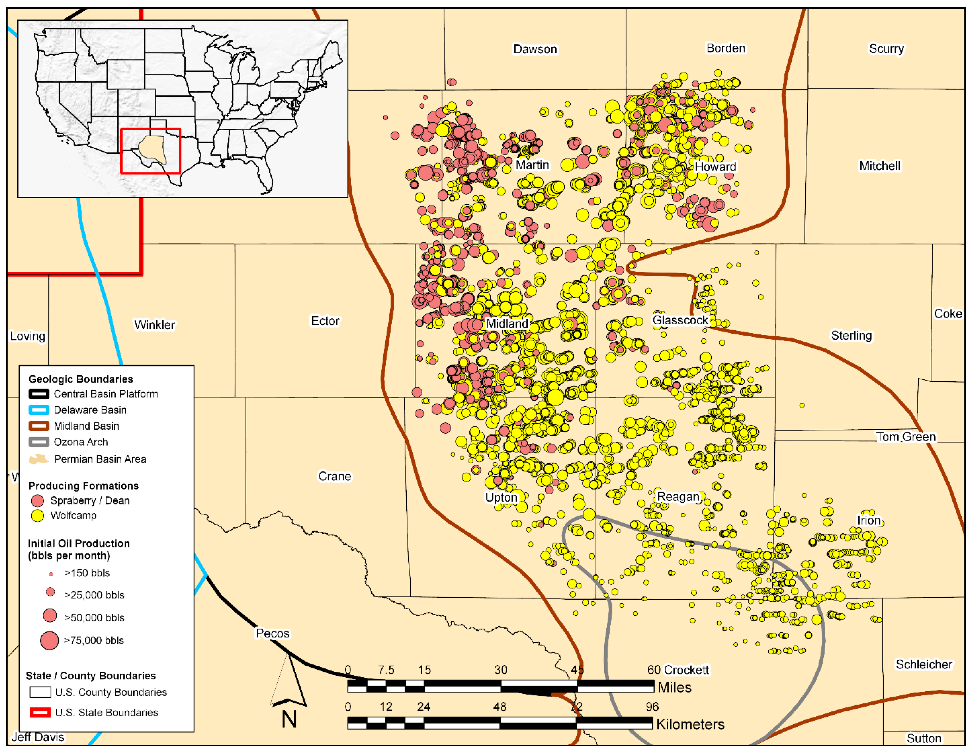
2.1. Study Area

| Era | Period | Epoch | Local Series | Stratigraphic/Formation Name | Reservoir Operational Name |
|---|---|---|---|---|---|
| Paleozoic | Permian | Guadalupian | Ward | San Andreas | San Andreas |
| San Angelo/Glorieta | San Angelo/ Glorieta | ||||
| Leonardian | Clearfork | Upper Leonard | |||
| Wichita | Upper Spraberry | Spraberry | |||
| Lower Spraberry | |||||
| Dean | |||||
| Lower Leonard | Wolfcamp | Wolfcamp A | |||
| Wolfcampian | Wolfcamp | Wolfcamp B | |||
| Wolfcamp C | |||||
| Pennsylvanian | Virgilian | Cisco/Cline | Wolfcamp D | ||
| Missourian | Canyon | Canyon | |||
| Des Moinesian | Strawn | Strawn | |||
| Atokan | Atoka/Bend | Atoka/Bend | |||
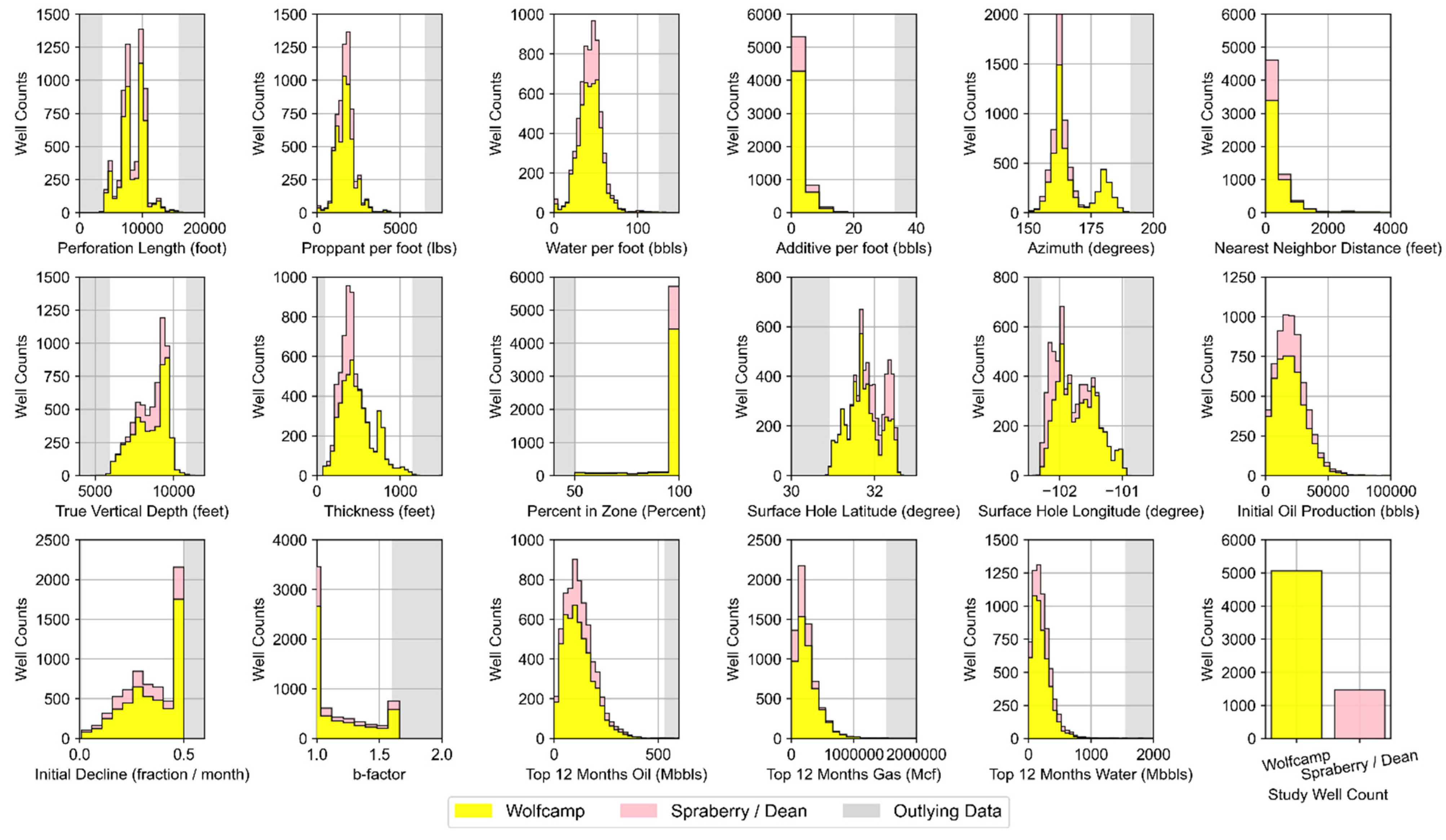
2.2. Study Data Overview and Data Processing
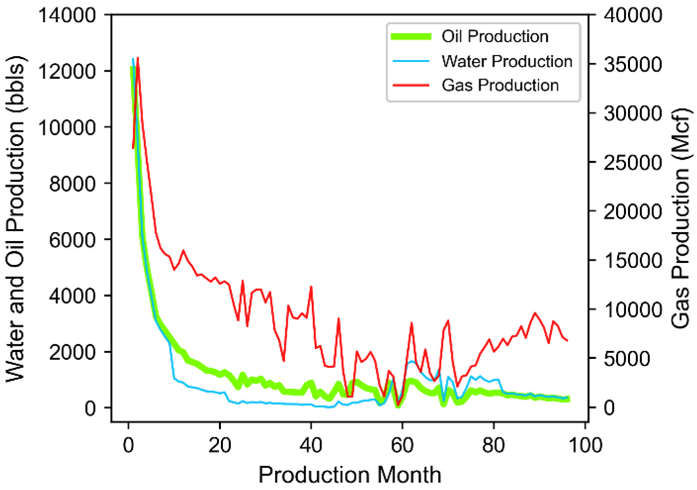
- Well Performance Attributes: These features relate to fluid production for wells in the study dataset. The dynamic features within the data group represent summation of the three-stream (oil, gas, and water) empirically-derived monthly values at the well level provided by DrillingInfo/Enverus. Data for these dynamic features is available for each month in a given well’s productive lifetime. Therefore, the volume of this data varies across wells depending on when they began production and how long wells are kept online. The “Top 12-months” static features for oil, gas, and water were derived via summation of the 12 largest observed values for each well based on monthly dynamic feature data. This approach has been implemented in our prior work [12,23] and has proven to effectively represent productivity potential for unconventional wells that may or may not have been subject to disruptions to their production time series profiles. Both the Top 12-months Oil and Gas features correlate strongly to well level estimated ultimate recover (EUR) as indicated in Figure 4. The static EUR features represent an estimation of the technically recoverable reserves at the well level. They are calculated by DrillingInfo/Enverus [87] using a combination of historic production data and a combination of Arps decline curve models [84].
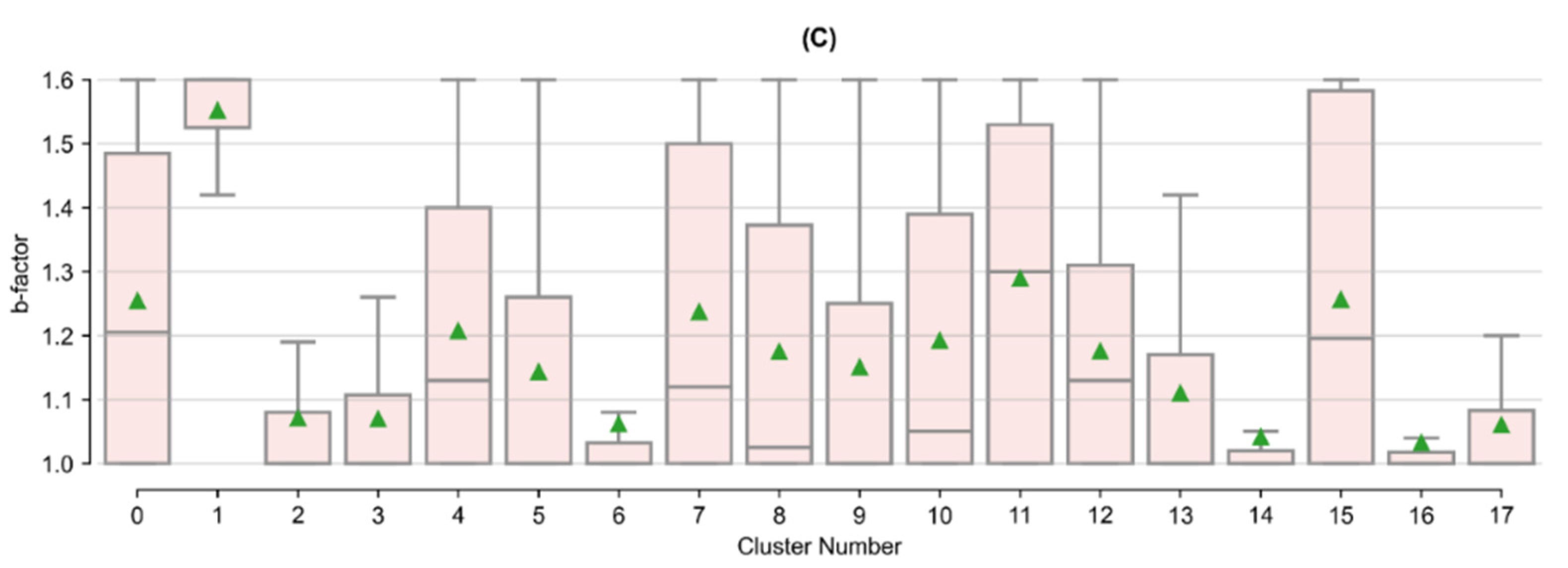
- Decline Curve Attributes: These features are inherent to decline curve analyses based on the Arps decline curve model [84]. The Arps model can be used to evaluate oil and/or gas declining production rates over time. Time-dependent reduction in hydrocarbon production can be attributed to reduced reservoir pressure as well as the relative change in the volumes of the produced fluids. The approach can also be used to forecast hydrocarbon production into the future. The Arps approach is based on fitting a mathematical decline model (either exponential, hyperbolic, or harmonic) to empirical observations of an asset’s (i.e., well) performance history [88]. Well features related to initial (oil) production, the initial decline, and degree of curvature (b-factor) are the parameters related to the Arps model. Values for these features for each well in the study dataset have been determined by Drillinginfo/Enverus [87]. The DrillingInfo/Enverus approach solves for the most appropriate Arps model parameters that minimize the sum of squared errors based on empirical production values for a given well [87]. DrillingInfo/Enverus restricts b-factors between 0 and 2. The b-factor is typically greater than 1 in unconventional shale plays given the inherent low permeability rock matrix and resulting extended duration of transient flow [89]; potentially a derivative of the bulk of empirical observations with shorter producing timeframes [90].
- Well Completion Attributes: These features pertain to each well’s design and completion attributes as it relates to well placement, orientation, and hydraulic fracturing design. The major hydraulic fracturing design features include the length of the perforated interval contacting the reservoir and the volume of proppant, water, and additive used for hydraulic fracturing normalized to a per foot of perforated interval basis. Proppant includes solids that may vary in size, shape or material type. They typically consist of sand or engineered materials (i.e., resin-coated sand or high-strength ceramic materials such as sintered bauxite) and are used to keep reservoir fractures open and conductive following hydraulic fracturing [91]. Additives may serve a variety of functions, with examples including the assurance of effective transport of water and proppant downhole and throughout the reservoir, as well as to ensure sustained hydrocarbon recovery after hydraulic fracturing. Specific components can tend to vary from one well to another and from operator to operator. However, example constituents include acids, friction reducers, biocides, pH adjusters, scale inhibitors, iron stabilizers, corrosion reducers, gelling agents, and cross-linking agents [92,93]. Other important well design characteristics captured in the dataset relate to the wellbore lateral orientation, spacing distance to nearby wells, and the portion of the horizontal perforated length within the targeted producing reservoir zone of interest. The directional alignment (reflected by azimuth) is often a design choice by field operators; one that is driven by the natural orientation of in situ stresses in targeted reservoir producing zones. Horizontal segments of wells that are drilled along the minimum horizontal stress often produce transverse fractures following horizontal fracturing. This form of fracturing may improve drainage efficiency. As a result, well laterals oriented properly on azimuth given natural in situ stress regimes may experience higher productivity [5,92]. Well azimuth was approximated based on the geographic orientation between each well’s surface hole latitude and longitude and lateral toe latitude and longitude. Well spacing may provide insight into the field operator’s anticipated drainage area based on the applied water and proppant intensity. Additionally, spacing-related data can be helpful in determining if closely-spaced wells suffer from possible interference from hydraulic fracturing operations (i.e., frack hits) or effects from parent/child well interactions [94,95] from nearby wells. We approximated the nearest well distance for each well in the dataset using the haversine formula and bottom hole latitude and longitude coordinates to its closest well neighbor prior to any dataset reduction. Percentage in zone is a metric which provides an indication of the wellbore geo-steering efficiency of the horizontal lateral component. DrillingInfo/Enverus provides this data readily for each well. Wells with a high portion of their perforated segment in the targeted producing zone are more likely to be better producers than those wells expected to deviate substantially off target. Each feature in this data group is treated as static. In actuality, many of these features, such as proppant, water, and additive per foot, could essentially vary over the life of any given well due to refracturing campaigns.
- Spatial and Reservoir Attributes: The features included attempt to best approximate the variability that may exist in the geologic conditions which influence hydrocarbon prominence and producibility that span the reservoirs of interest across the study domain. True vertical depth and thickness (i.e., reservoir thickness) are provided from DillingInfo/Enverus for each well. However, other relevant geologic characteristics that are known to influence hydrocarbon production, such as total organic carbon, porosity, hydrocarbon and/or water saturation, thermal maturity, reservoir pressure, existence of fracture networks, and capacity of the reservoir(s) to be hydraulically fractured [96,97,98,99], are not directly or readily available in bulk. Additionally, many of these features are dynamic in nature and change over the duration of hydrocarbon production (such as fluid saturation and pressure in the reservoir), while others essentially remain static (such as porosity and thermal maturity) [100]. Each well’s locational data (surface latitude and longitude) is used as a contingency means to approximate geologic conditional variability known to vary spatially across the study area—an approach widely used in other ML-based model development efforts occurring over large spatial horizons [22,26,27,101].

2.3. Data Preprocessing Prior to Model Training and Testing
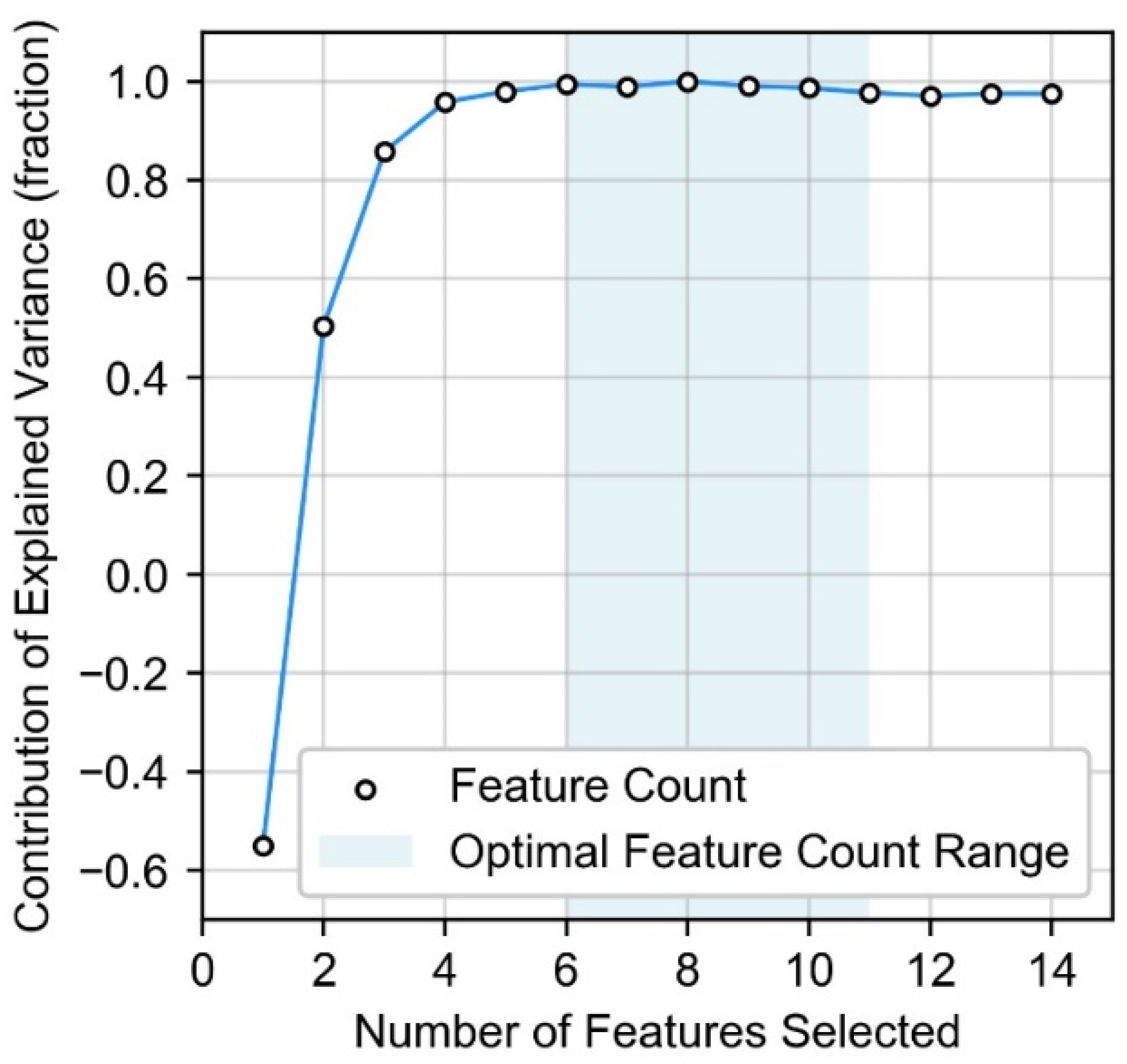
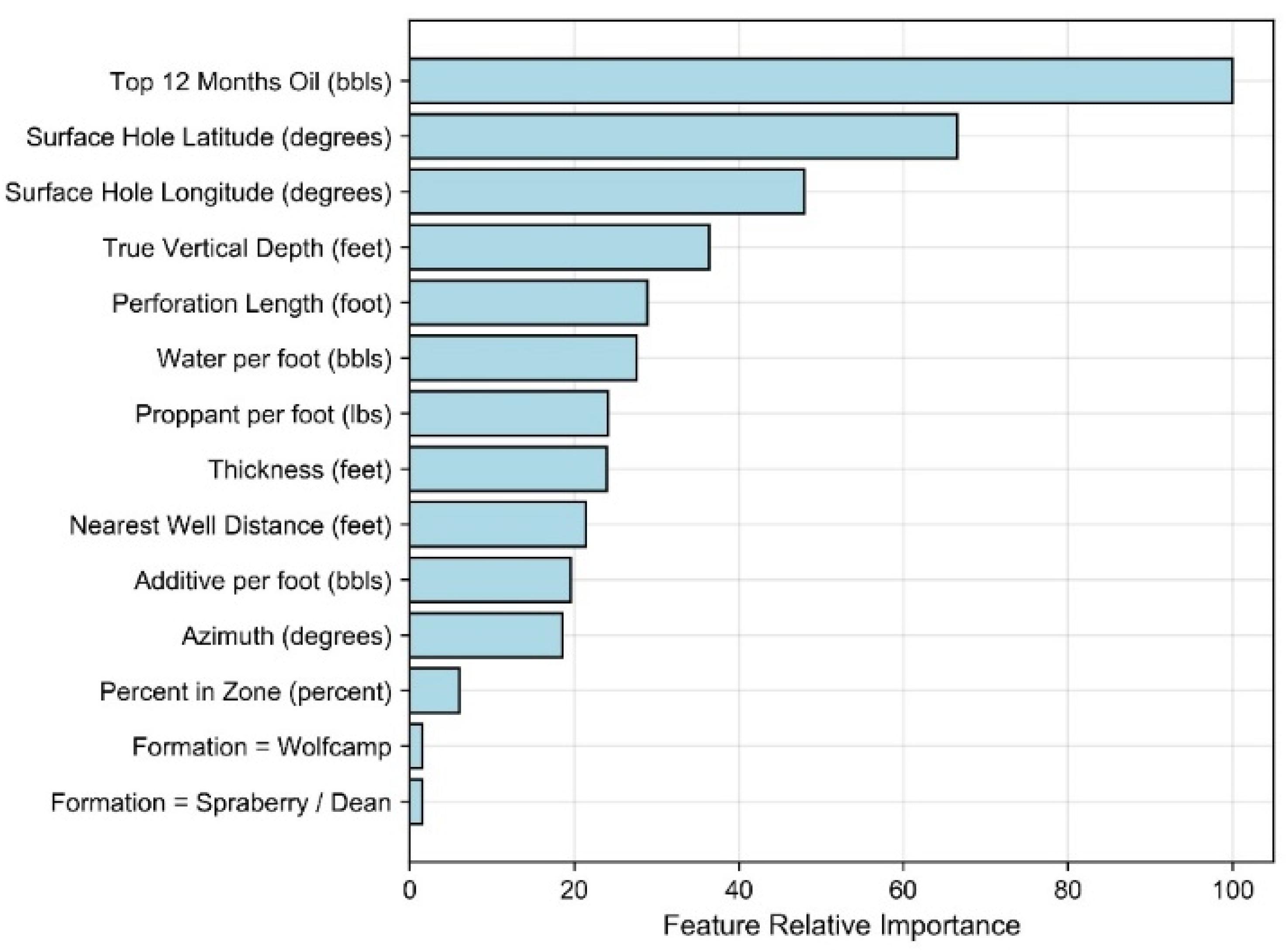
2.4. Feature Selection Approach
2.5. Machine Learning Model Development and Evaluation
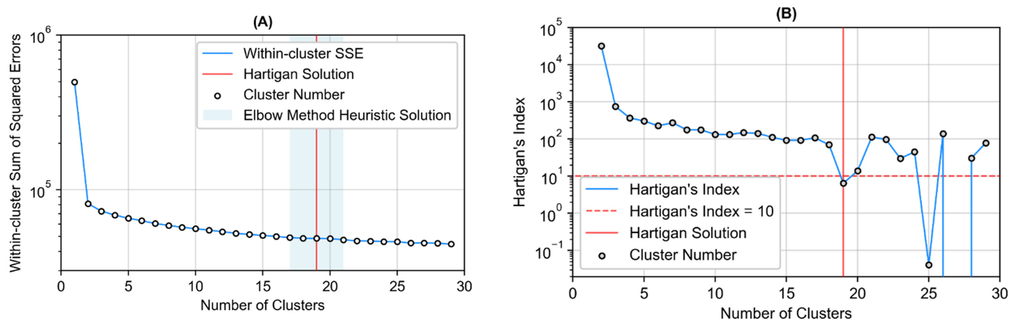
2.5.1. Clustering Evaluation
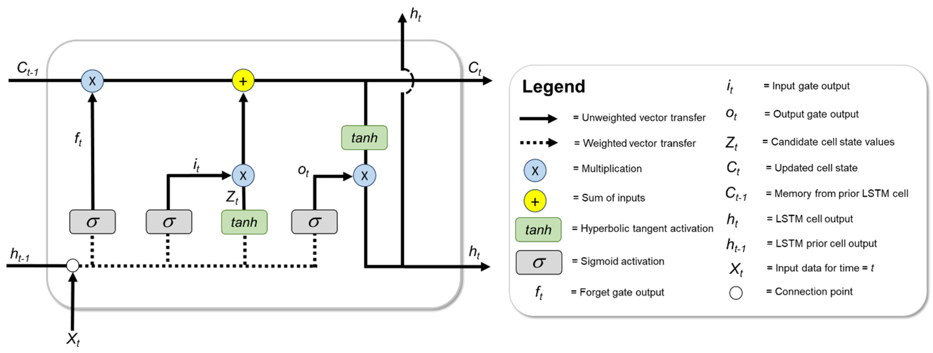
2.5.2. Time Series Joint Associated Fluid Production Model
- First, the forget game (ft) is utilized to determine information that becomes omitted away from the cell state. New information introduced to the LSTM memory cell via ht−1 and Xt undergoes sigmoid transformation, the result of which is output between 0 (becomes fully omitted) and 1 (becomes fully included) for each number in the cell state Ct−1 per Equation (5).
- The second step involves determining new information to be stored in the cell state; this step occurs through two separate parts. The input gate (it) applies sigmoid activation to ht−1 and Xt and is used to inform values that will be updated in the cell state per Equation (6). Additionally, tanh activation generates a vector of new candidate values (Zt), which could be included in the cell state per Equation (7).
- The prior cell state Ct−1 is updated with new information to a new cell state Ct, via Equation (8):
- The final step generates output (ht) that leverages memory from the cell. The output is a function of the new cell state Ct that undergoes some filtering via tanh activation as well as from output from the output gate (ot). The mathematical expressions for these steps are presented in Equations (9) and (10).
2.5.3. Model Performance Evaluation
2.6. Oil Forecasting
3. Results and Discussion
3.1. Feature Selection Results
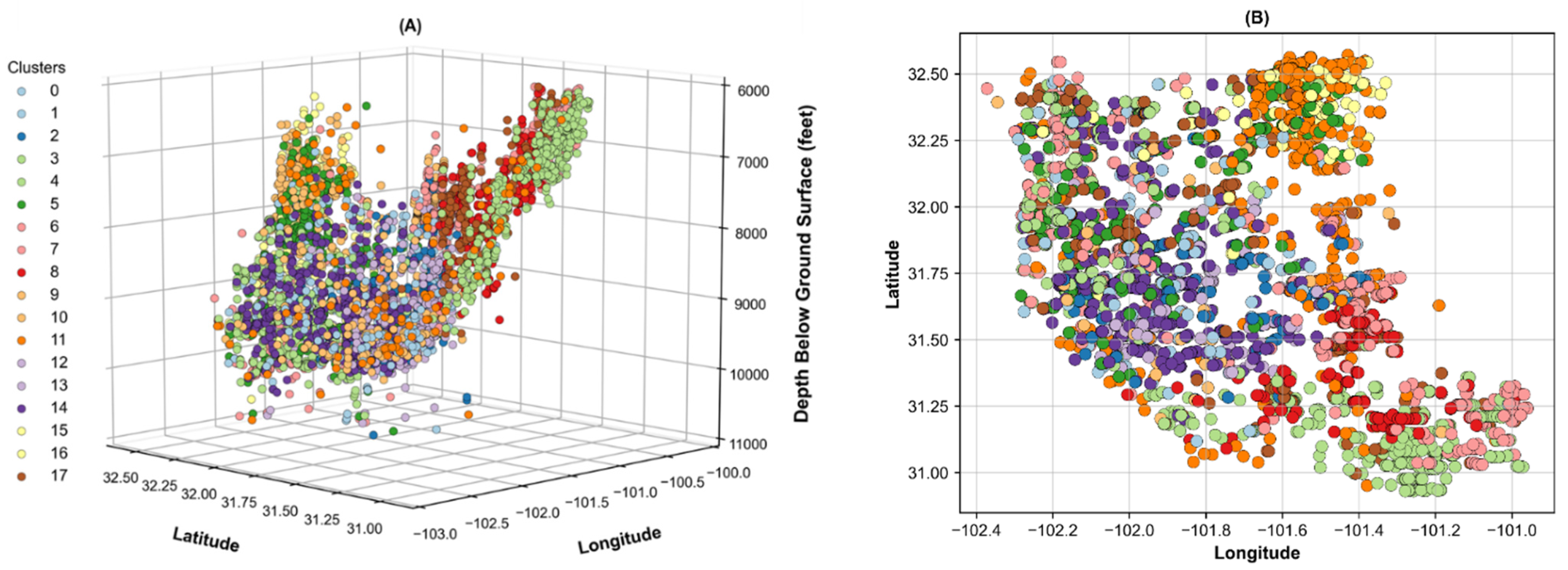
3.2. Cluster Analysis
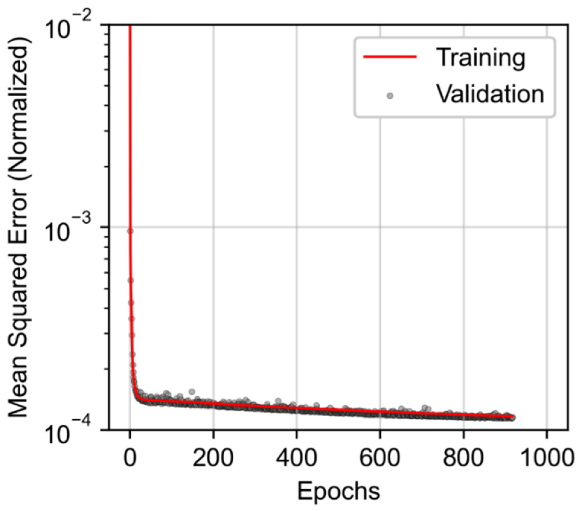
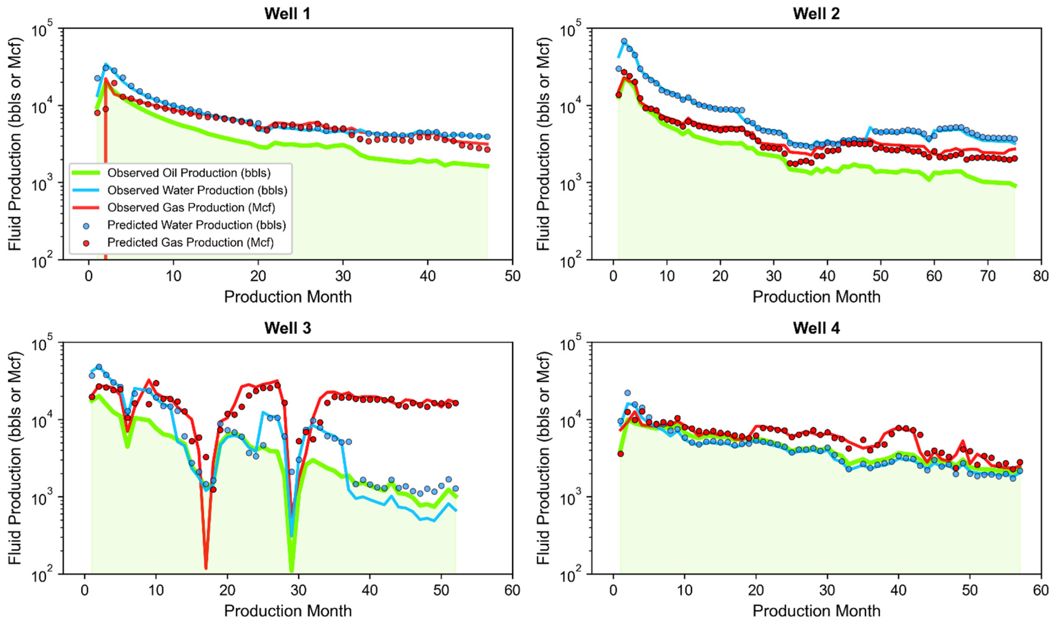
3.3. Joint Associated Fluid Production Model Training and Performance
- Well 1: Located in central Martin County producing from the Lower Spraberry with an 8409-foot perforated length, and placed at a total vertical depth of 9334 feet below ground surface.
- Well 2: Located in northern central Midland County producing from the Wolfcamp B with a 7142-foot perforated length, and placed at a total vertical depth of 9673 feet below ground surface.
- Well 3: Located in southeastern Midland County producing from the Wolfcamp B with a 6722-foot perforated length, and placed at a total vertical depth of 9383 feet below ground surface.
- Well 4: Located in western Martin County producing from the Wolfcamp C with a 4855-foot perforated length, and placed at a total vertical depth of 10,031 feet below ground surface.

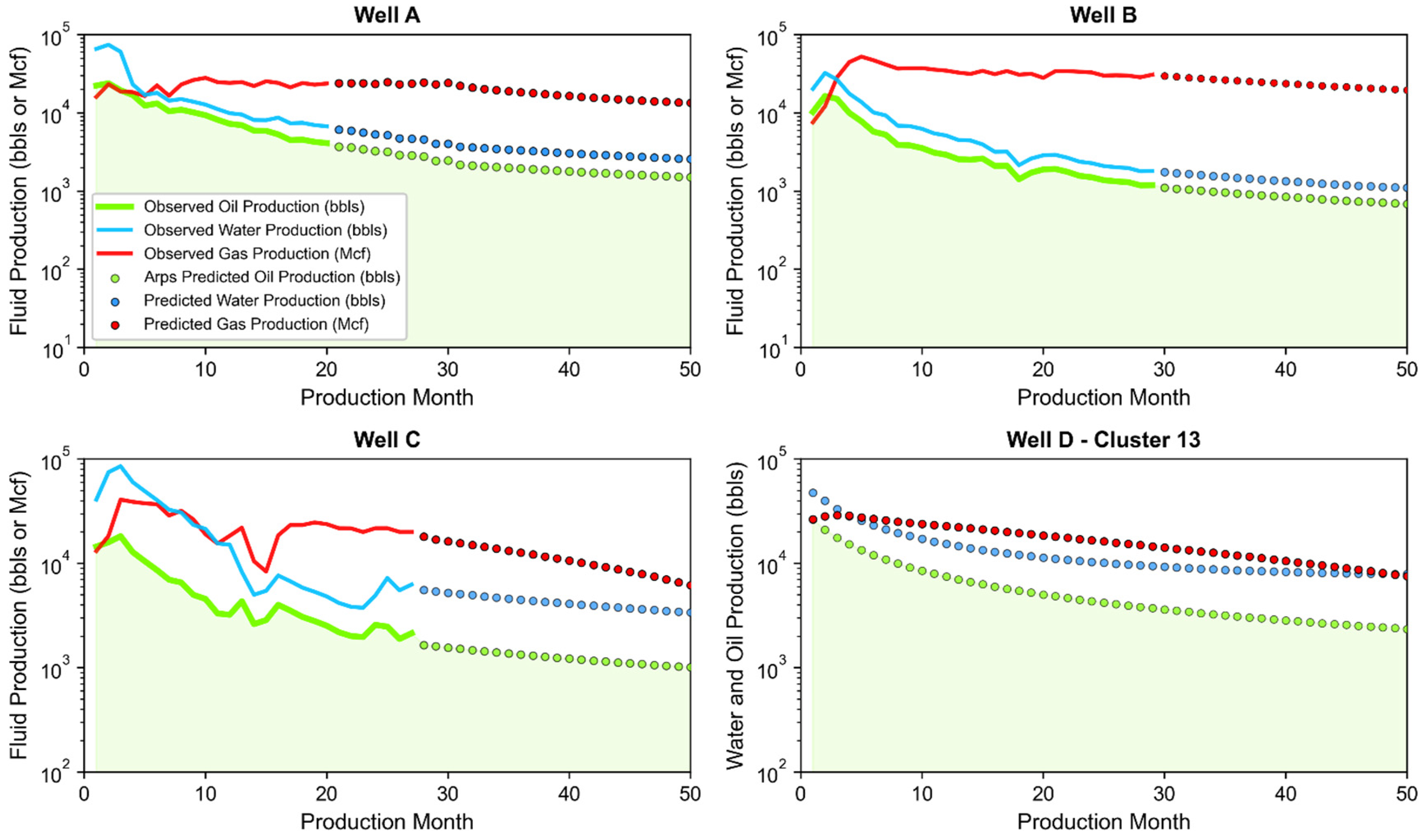
- Well A: Located in northern Upton County producing from the Wolfcamp A with a 7745-foot perforated length, and placed at a total vertical depth of 9476 feet below ground surface.
- Well B: Located in western Irion County producing from the Wolfcamp B with a 10,114-foot perforated length, and placed at a total vertical depth of 6709 feet below ground surface.
- Well C: Located in southern Glasscock County producing from the Wolfcamp A with a 10,261-foot perforated length, and placed at a total vertical depth of 7976 feet below ground surface.
- Well D: Theoretical well representative of Cluster 13 (see Table A2 in Appendix C for specifics) based on a 9870-foot perforated length, an initial monthly oil production of 26,324 bbls, and placed at a total vertical depth of 9128 feet below ground surface.
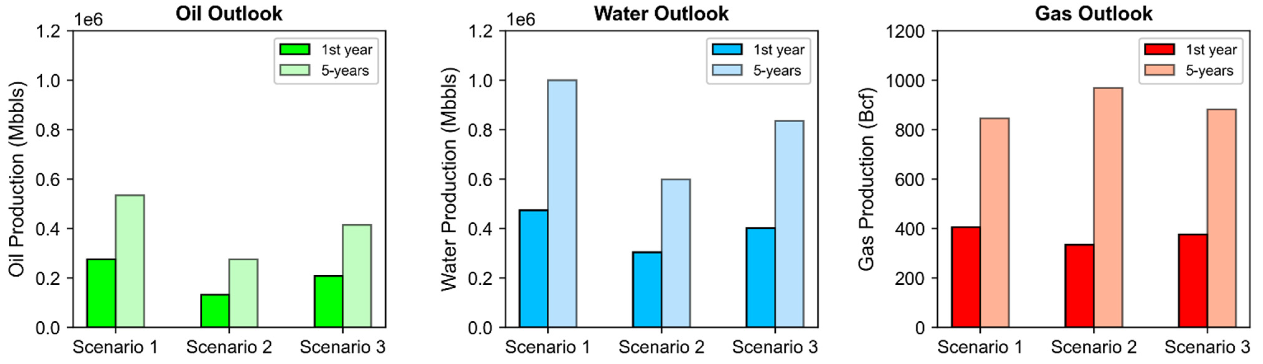
4. Oil, Gas, and Water Production Outlook
- Scenario 1: high efficiency development—25 percent contribution of wells from clusters 3, 5, 11, and 16
- Scenario 2: low efficiency development—20 percent contribution of wells from clusters 1, 4, 6, 8, and 17
- Scenario 3: diversified development—contribution of wells from each cluster randomly assigned under equal probability per cluster
5. Conclusions
Author Contributions
Funding
Institutional Review Board Statement
Informed Consent Statement
Data Availability Statement
Acknowledgments
Conflicts of Interest
Unit Conversions
Appendix A. Feature Selection Results Overview
Appendix B. Tukey’s Test Results on Arps Attributes by Cluster
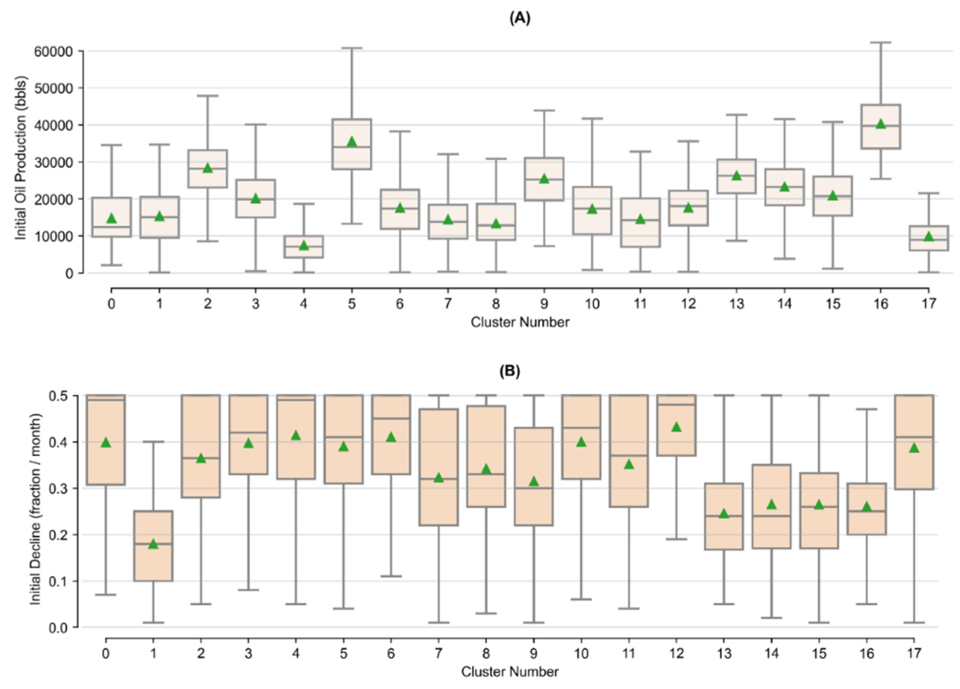
| Cluster Number | Initial Oil Production (bbls) | Initial Decline (Fraction/Month) | b-Factor | |||||||
|---|---|---|---|---|---|---|---|---|---|---|
| Count | Mean | Stdev. | Tukey’s Group | Mean | Stdev. | Tukey’s Group | Mean | Stdev. | Tukey’s Group | |
| 0 | 84 | 14,816 | 7459 | H, I, J, K | 0.40 | 0.12 | A, B, C, D | 1.25 | 0.24 | B, C, D, E |
| 1 | 259 | 15,364 | 7653 | J, K | 0.18 | 0.09 | H | 1.55 | 0.08 | A |
| 2 | 246 | 28,382 | 7826 | C | 0.36 | 0.12 | D, E | 1.07 | 0.14 | I, J |
| 3 | 594 | 20,148 | 7935 | G | 0.40 | 0.11 | B | 1.07 | 0.13 | I, J |
| 4 | 460 | 7481 | 4835 | M | 0.41 | 0.12 | A, B | 1.21 | 0.22 | C, D, E, F |
| 5 | 574 | 35,577 | 10,694 | B | 0.39 | 0.11 | B, C, D | 1.14 | 0.20 | G, H |
| 6 | 328 | 17,625 | 7588 | H, I | 0.41 | 0.10 | A, B | 1.06 | 0.13 | I, J |
| 7 | 609 | 14,442 | 7392 | K | 0.32 | 0.14 | F | 1.24 | 0.25 | B, C |
| 8 | 230 | 13,408 | 7594 | K | 0.34 | 0.12 | E, F | 1.17 | 0.22 | D, E, F, G |
| 9 | 173 | 25,506 | 8124 | D, E | 0.32 | 0.13 | F | 1.15 | 0.23 | F, G, H |
| 10 | 515 | 17,353 | 8606 | H, I, J | 0.40 | 0.11 | B | 1.19 | 0.23 | E, F |
| 11 | 101 | 14,630 | 8813 | I, J, K | 0.35 | 0.13 | C, D, E, F | 1.29 | 0.24 | B |
| 12 | 485 | 17,666 | 6449 | H | 0.43 | 0.08 | A | 1.18 | 0.18 | F, G |
| 13 | 304 | 26,324 | 6777 | C, D | 0.25 | 0.11 | G | 1.11 | 0.18 | H, I |
| 14 | 554 | 23,346 | 7579 | E, F | 0.27 | 0.13 | G | 1.04 | 0.09 | J |
| 15 | 160 | 20,971 | 8156 | F, G | 0.26 | 0.12 | G | 1.26 | 0.25 | B, C |
| 16 | 346 | 40,342 | 8293 | A | 0.26 | 0.10 | G | 1.03 | 0.08 | J |
| 17 | 188 | 9959 | 5386 | L | 0.39 | 0.11 | B, C, D | 1.06 | 0.11 | I, J |
Appendix C. Well Cluster Statics and Production Outlooks
| Data Group | Dataset Feature | Statistic | Midland Basin Well Cluster Number: 0 through 8 | ||||||||
| 0 | 1 | 2 | 3 | 4 | 5 | 6 | 7 | 8 | |||
| Well Completion Attributes | Perforation Length (foot) | Mean | 6782 | 8791 | 9593 | 7928 | 7719 | 10,061 | 9177 | 7139 | 9663 |
| Stdev. | 1990 | 1770 | 1319 | 1665 | 1563 | 1502 | 1856 | 1565 | 1763 | ||
| IQR | 2985 | 2704 | 1132 | 2378 | 1065 | 756 | 2581 | 1545 | 1756 | ||
| Proppant per foot (lbs) | Mean | 1818 | 1698 | 1764 | 1659 | 1303 | 1845 | 1938 | 1477 | 2283 | |
| Stdev. | 570 | 391 | 331 | 349 | 413 | 389 | 428 | 395 | 394 | ||
| IQR | 487 | 468 | 319 | 430 | 495 | 367 | 459 | 517 | 546 | ||
| Water per foot (bbls) | Mean | 46.8 | 45.6 | 50.7 | 40.6 | 28.2 | 47.8 | 49.6 | 37.2 | 51.4 | |
| Stdev. | 15.3 | 10.3 | 9.0 | 12.2 | 8.3 | 10.1 | 10.9 | 10.6 | 9.3 | ||
| IQR | 9.8 | 12.4 | 11.6 | 15.5 | 9.1 | 13.0 | 13.1 | 13.2 | 8.7 | ||
| Additive per foot (bbls) | Mean | 12.1 | 2.8 | 2.9 | 4.1 | 1.8 | 2.6 | 3.5 | 3.2 | 2.1 | |
| Stdev. | 3.9 | 1.8 | 1.5 | 3.1 | 1.3 | 1.6 | 3.3 | 1.8 | 1.2 | ||
| IQR | 3.9 | 2.5 | 2.0 | 4.9 | 2.1 | 2.3 | 2.5 | 2.6 | 1.3 | ||
| Azimuth (degrees) | Mean | 165.1 | 162.4 | 162.6 | 162.6 | 180.3 | 162.6 | 178.9 | 162.6 | 180.8 | |
| Stdev. | 7.0 | 3.7 | 3.7 | 3.6 | 3.4 | 3.3 | 5.9 | 3.3 | 3.1 | ||
| IQR | 3.2 | 4.2 | 3.4 | 4.1 | 4.3 | 4.0 | 5.1 | 2.3 | 4.1 | ||
| Nearest Well Distance (feet) | Mean | 844 | 288 | 254 | 261 | 550 | 259 | 523 | 382 | 388 | |
| Stdev. | 1013 | 384 | 307 | 324 | 473 | 269 | 441 | 556 | 428 | ||
| IQR | 1185 | 307 | 277 | 267 | 519 | 295 | 413 | 390 | 453 | ||
| Decline Curve Attributes | Initial Oil Production (bbls) | Mean | 14,816 | 15,364 | 28,382 | 20,148 | 7481 | 35,577 | 17,625 | 14,442 | 13,408 |
| Stdev. | 7459 | 7653 | 7826 | 7935 | 4835 | 10,694 | 7588 | 7392 | 7594 | ||
| IQR | 10,635 | 11,155 | 10,173 | 10,197 | 5895 | 13,455 | 10,748 | 9233 | 9916 | ||
| Initial Decline (fraction/month) | Mean | 0.40 | 0.18 | 0.36 | 0.40 | 0.41 | 0.39 | 0.41 | 0.32 | 0.34 | |
| Stdev. | 0.12 | 0.09 | 0.12 | 0.11 | 0.12 | 0.11 | 0.10 | 0.14 | 0.12 | ||
| IQR | 0.20 | 0.15 | 0.22 | 0.17 | 0.18 | 0.19 | 0.17 | 0.26 | 0.22 | ||
| b-factor | Mean | 1.25 | 1.55 | 1.07 | 1.07 | 1.21 | 1.14 | 1.06 | 1.24 | 1.17 | |
| Stdev. | 0.24 | 0.08 | 0.14 | 0.13 | 0.22 | 0.20 | 0.13 | 0.25 | 0.22 | ||
| IQR | 0.50 | 0.08 | 0.08 | 0.11 | 0.40 | 0.26 | 0.04 | 0.50 | 0.39 | ||
| Spatial and Reservoir Attributes | True Vertical Depth (feet) | Mean | 8924 | 8964 | 8947 | 9310 | 7112 | 8811 | 7150 | 9020 | 7460 |
| Stdev. | 752 | 630 | 626 | 470 | 741 | 785 | 620 | 771 | 577 | ||
| IQR | 798 | 848 | 884 | 563 | 963 | 1296 | 1018 | 1174 | 686 | ||
| Thickness (feet) | Mean | 443 | 398 | 471 | 320 | 774 | 375 | 633 | 374 | 553 | |
| Stdev. | 157 | 137 | 115 | 96 | 146 | 108 | 207 | 134 | 191 | ||
| IQR | 209 | 148 | 137 | 148 | 59 | 136 | 338 | 185 | 361 | ||
| Surface Hole Latitude (degrees) | Mean | 31.64 | 31.92 | 31.70 | 32.08 | 31.15 | 32.08 | 31.38 | 31.98 | 31.32 | |
| Stdev. | 0.32 | 0.28 | 0.17 | 0.26 | 0.12 | 0.28 | 0.23 | 0.29 | 0.14 | ||
| IQR | 0.44 | 0.45 | 0.19 | 0.47 | 0.19 | 0.47 | 0.38 | 0.56 | 0.19 | ||
| Surface Hole Longitude (degrees) | Mean | −101.93 | −101.93 | −101.81 | −102.08 | −101.33 | −101.87 | −101.26 | −101.90 | −101.58 | |
| Stdev. | 0.28 | 0.19 | 0.22 | 0.14 | 0.23 | 0.24 | 0.18 | 0.29 | 0.16 | ||
| IQR | 0.32 | 0.29 | 0.32 | 0.21 | 0.26 | 0.42 | 0.30 | 0.53 | 0.15 | ||
| Wolfcamp | Count | 68 | 168 | 223 | 315 | 456 | 419 | 326 | 445 | 230 | |
| S.berry/Dean | Count | 16 | 91 | 23 | 280 | 4 | 155 | 2 | 164 | 0 | |
| Production Forecast per Well | Cumulative Oil (Mbbls) | 1st year | 77 | 111 | 147 | 100 | 38 | 181 | 86 | 82 | 73 |
| 5-years | 154 | 282 | 275 | 183 | 74 | 346 | 156 | 169 | 145 | ||
| Cumulative Gas (Bcf) | 1st year | 0.16 | 0.20 | 0.25 | 0.15 | 0.12 | 0.27 | 0.25 | 0.13 | 0.22 | |
| 5-years | 0.29 | 0.58 | 0.62 | 0.23 | 0.23 | 0.60 | 0.76 | 0.21 | 0.79 | ||
| Cumulative Water (Mbbls) | 1st year | 154 | 230 | 268 | 181 | 102 | 304 | 200 | 162 | 182 | |
| 5-years | 289 | 587 | 545 | 347 | 175 | 659 | 358 | 324 | 328 | ||
| Data Group | Dataset Feature | Statistic | Midland Basin Well Cluster Number: 9 through 17 | ||||||||
| 9 | 10 | 11 | 12 | 13 | 14 | 15 | 16 | 17 | |||
| Well Completion Attributes | Perforation Length (foot) | Mean | 8307 | 7677 | 7253 | 7225 | 9870 | 8762 | 9448 | 9972 | 7417 |
| Stdev. | 1814 | 1970 | 2103 | 1794 | 1155 | 1469 | 1892 | 1333 | 1605 | ||
| IQR | 2711 | 2933 | 4212 | 2361 | 563 | 2313 | 2612 | 740 | 1549 | ||
| Proppant per foot (lbs) | Mean | 3281 | 1728 | 1609 | 1441 | 1752 | 1812 | 1787 | 1828 | 1342 | |
| Stdev. | 775 | 464 | 535 | 547 | 336 | 359 | 412 | 490 | 394 | ||
| IQR | 872 | 677 | 759 | 687 | 305 | 413 | 507 | 407 | 532 | ||
| Water per foot (bbls) | Mean | 71.4 | 39.4 | 40.6 | 36.6 | 49.4 | 48.8 | 44.9 | 48.0 | 32.8 | |
| Stdev. | 19.7 | 11.2 | 14.9 | 14.0 | 8.0 | 10.7 | 12.5 | 10.2 | 8.6 | ||
| IQR | 23.2 | 13.8 | 17.3 | 18.9 | 8.7 | 9.6 | 15.5 | 10.6 | 7.8 | ||
| Additive per foot (bbls) | Mean | 4.9 | 2.1 | 4.2 | 2.1 | 2.2 | 2.3 | 2.1 | 2.9 | 1.9 | |
| Stdev. | 2.9 | 1.5 | 3.4 | 1.3 | 1.4 | 1.5 | 1.5 | 1.7 | 1.2 | ||
| IQR | 3.0 | 1.8 | 3.8 | 1.6 | 2.0 | 2.3 | 2.0 | 1.9 | 2.0 | ||
| Azimuth (degrees) | Mean | 163.2 | 162.6 | 168.0 | 162.2 | 162.9 | 162.4 | 163.3 | 162.8 | 180.8 | |
| Stdev. | 5.5 | 2.9 | 8.8 | 3.3 | 3.7 | 3.4 | 3.3 | 3.6 | 2.1 | ||
| IQR | 4.6 | 2.5 | 17.6 | 3.6 | 3.5 | 3.8 | 3.2 | 4.4 | 2.2 | ||
| Nearest Well Distance (feet) | Mean | 395 | 392 | 5658 | 303 | 328 | 243 | 486 | 278 | 343 | |
| Stdev. | 542 | 473 | 1942 | 354 | 308 | 306 | 764 | 270 | 438 | ||
| IQR | 419 | 404 | 2770 | 285 | 386 | 259 | 511 | 316 | 438 | ||
| Decline Curve Attributes | Initial Oil Production (bbls) | Mean | 25,506 | 17,353 | 14,630 | 17,666 | 26,324 | 23,346 | 20,971 | 40,342 | 9959 |
| Stdev. | 8124 | 8606 | 8813 | 6449 | 6777 | 7579 | 8156 | 8293 | 5386 | ||
| IQR | 11,762 | 12,799 | 13,555 | 9324 | 9246 | 9785 | 10,744 | 11,795 | 6533 | ||
| Initial Decline (fraction/month) | Mean | 0.32 | 0.40 | 0.35 | 0.43 | 0.25 | 0.27 | 0.26 | 0.26 | 0.39 | |
| Stdev. | 0.13 | 0.11 | 0.13 | 0.08 | 0.11 | 0.13 | 0.12 | 0.10 | 0.11 | ||
| IQR | 0.21 | 0.18 | 0.25 | 0.13 | 0.15 | 0.18 | 0.17 | 0.11 | 0.21 | ||
| b-factor | Mean | 1.15 | 1.19 | 1.29 | 1.18 | 1.11 | 1.04 | 1.26 | 1.03 | 1.06 | |
| Stdev. | 0.23 | 0.23 | 0.24 | 0.18 | 0.18 | 0.09 | 0.25 | 0.08 | 0.11 | ||
| IQR | 0.26 | 0.39 | 0.54 | 0.31 | 0.17 | 0.02 | 0.59 | 0.02 | 0.09 | ||
| Spatial and Reservoir Attributes | True Vertical Depth (feet) | Mean | 9078 | 7883 | 8340 | 9238 | 9128 | 9123 | 7751 | 8963 | 7523 |
| Stdev. | 609 | 568 | 1101 | 465 | 424 | 511 | 727 | 587 | 723 | ||
| IQR | 784 | 527 | 1950 | 555 | 540 | 673 | 956 | 962 | 961 | ||
| Thickness (feet) | Mean | 503 | 384 | 463 | 541 | 653 | 380 | 369 | 356 | 477 | |
| Stdev. | 209 | 103 | 183 | 145 | 176 | 103 | 111 | 86 | 151 | ||
| IQR | 244 | 132 | 224 | 168 | 289 | 119 | 110 | 115 | 254 | ||
| Surface Hole Latitude (degrees) | Mean | 31.83 | 32.23 | 31.80 | 31.68 | 31.60 | 31.91 | 32.33 | 32.09 | 31.39 | |
| Stdev. | 0.33 | 0.30 | 0.48 | 0.16 | 0.16 | 0.27 | 0.24 | 0.24 | 0.18 | ||
| IQR | 0.56 | 0.47 | 0.87 | 0.24 | 0.26 | 0.43 | 0.21 | 0.39 | 0.27 | ||
| Surface Hole Longitude (degrees) | Mean | −101.90 | −101.58 | −101.70 | −101.89 | −101.82 | −102.01 | −101.62 | −101.94 | −101.38 | |
| Stdev. | 0.20 | 0.14 | 0.32 | 0.15 | 0.12 | 0.16 | 0.22 | 0.19 | 0.17 | ||
| IQR | 0.25 | 0.12 | 0.56 | 0.18 | 0.15 | 0.19 | 0.27 | 0.37 | 0.17 | ||
| Wolfcamp | Count | 137 | 356 | 89 | 459 | 301 | 321 | 88 | 227 | 188 | |
| S.berry/Dean | Count | 36 | 159 | 12 | 26 | 3 | 223 | 72 | 119 | 0 | |
| Production Forecast per Well | Cumulative Oil (Mbbls) | 1st year | 141 | 89 | 80 | 87 | 160 | 135 | 129 | 237 | 50 |
| 5-years | 281 | 173 | 168 | 167 | 328 | 265 | 279 | 465 | 91 | ||
| Cumulative Gas (Bcf) | 1st year | 0.26 | 0.14 | 0.12 | 0.15 | 0.31 | 0.22 | 0.22 | 0.34 | 0.12 | |
| 5-years | 0.57 | 0.19 | 0.16 | 0.27 | 0.91 | 0.50 | 0.45 | 0.85 | 0.27 | ||
| Cumulative Water (Mbbls) | 1st year | 271 | 185 | 170 | 171 | 306 | 249 | 265 | 373 | 111 | |
| 5-years | 574 | 364 | 287 | 332 | 684 | 515 | 621 | 879 | 178 | ||
References
- U.S. Department of Energy. Ethane Storage and Distribution Hub in the United States; U.S. DOE: Washington, DC, USA, 2018.
- Pirog, R.; Ratner, M. Natural Gas in the U.S. Economy: Opportunities for Growth; Congressional Research Service: Washington, DC, USA, 2012.
- U.S. Energy Information Administration. Today in Energy: Both Natural Gas Supply and Demand Have Increased from Year-Ago Levels. U.S. Department of Energy. 4 October 2018. Available online: https://www.eia.gov/todayinenergy/detail.php?id=37193 (accessed on 31 March 2019).
- Clemente, J.U.S. Natural Gas Demand for Electricity Can Only Grow. Forbes. 15 January 2019. Available online: https://www.forbes.com/sites/judeclemente/2019/01/15/u-s-natural-gas-demand-for-electricity-can-only-grow/#27b0ba844c74 (accessed on 31 March 2019).
- Aadnøy, B.; Looyeh, R. Petroleum Rock Mechanics, 2nd ed.; Gulf Professional Publishing: Oxford, UK, 2019. [Google Scholar]
- United States Geological Survey, U.S. Department of the Interior. What Is Hydraulic Fracturing? Available online: https://www.usgs.gov/faqs/what-hydraulic-fracturing?qt-news_science_products=0#qt-news_science_products (accessed on 21 November 2020).
- Hyman, J.; Jiménez-Martínez, J.; Viswanathan, H.; Carey, J.P.M.; Rougier, E.; Karra, S.; Kang, Q.; Frash, L.; Chen, L.; Lei, Z.; et al. Understanding hydraulic fracturing: Amulti-scale problem. Philos. Trans. Ser. A Math. Phys. Eng. Sci. 2016, 374, 20150426. [Google Scholar] [CrossRef] [PubMed]
- Aminzadeh, F. Hydraulic Fracturing, An Overview. J. Sustain. Energy Eng. 2019, 6, 204–228. [Google Scholar] [CrossRef]
- U.S. Environmental Protection Agency. The Process of Unconventional Natural Gas Production. 22 January 2020. Available online: https://www.epa.gov/uog/process-unconventional-natural-gas-production (accessed on 21 November 2020).
- Perrin, J. Horizontally Drilled Wells Dominate U.S. Tight Formation Production. U.S. Energy Information Administration. 6 June 2019. Available online: https://www.eia.gov/todayinenergy/detail.php?id=39752 (accessed on 12 December 2020).
- van Wagener, D.; Aloulou, F. Tight Oil Development Will Continue to Drive Future U.S. Crude Oil Production. U.S. Energy Information Administration, 28 March 2019. Available online: https://www.eia.gov/todayinenergy/detail.php?id=38852 (accessed on 12 December 2020).
- Vikara, D.; Remson, D.; Khanna, V. Machine learning-informed ensemble framework for evaluating shale gas production potential: Case study in the Marcellus Shale. J. Nat. Gas Sci. Eng. 2020, 84, 103679. [Google Scholar] [CrossRef]
- U.S. Department of Energy. Quadrennial Technology Review 2015—Chapter 7: Advancing Systems and Technologies to Produce Clearner Fuels; U.S. Department of Energy: Washington, DC, USA, 2015.
- Mehrotra, R.; Gopalan, R. Factors Influencing Strategic Decision-Making Process for the Oil/Gas Industris of UAE—A study. Int. J. Mark. Financ. Manag. 2017, 5, 62–69. [Google Scholar]
- Mo, S.; Zhu, Y.; Zabaras, N.; Shi, X.; Wu, J. Deep convolutional encoder-decoder networks for uncertainty quantification of dynamic multiphase flow in heterogeneous media. Water Resour. Res. 2019, 55, 703–728. [Google Scholar] [CrossRef]
- Esmaili, S.; Mohaghegh, S. Full field reservoir modeling of shale assets using advanced data-driven analytics. Geosci. Front. 2016, 7, 11–20. [Google Scholar] [CrossRef] [Green Version]
- McGlade, C.; Speirs, J.; Sorrell, S. Methods of estimating shale gas resources—Comparison, evaluation and implications. Energy 2013, 59, 116–125. [Google Scholar] [CrossRef] [Green Version]
- Baaziz, A.; Quoniam, L. How to use Big Data technologies to optimize operations in Upstream Petroleum Industry. In Proceedings of the 21st World Petroleum Congress, Moscow, Russia, 15–19 June 2014. [Google Scholar]
- Bettin, G.; Bromhal, G.; Brudzinski, M.; Cohen, A.; Guthrie, G.; Johnson, P.; Matthew, L.; Mishra, S.; Vikara, D. Real-Time Decision Making for the Subsurface Report; Carnegie Mellon University Wilson E. Scott Institute for Energy Innovation: Pittsburgh, PA, USA, 2019. [Google Scholar]
- Mishra, S.; Lin, L. Application of Data Analytics for Production Optimization in Unconventional Reservoirs: A Critical Review. In Proceedings of the Unconventional Resources Technology Conference, Austin, TX, USA, 24–26 July 2017. [Google Scholar]
- Abubakar, A. Potential and Challenges of Applying Artificial Intelligence and Machine-Learning Methods for Geoscience; Society of Exploration Geophysicists: Houston, TX, USA, 2020. [Google Scholar]
- Wang, S.; Chen, S. Insights to fracture stimulation design in unconventional reservoirs based on machine learning modeling. J. Pet. Sci. Eng. 2019, 174, 682–695. [Google Scholar] [CrossRef]
- Vikara, D.; Remson, D.; Khanna, V. Gaining Perspective on Unconventional Well Design Choices through Play-level Application of Machine Learning Modeling. Upstream Oil Gas Technol. 2020, 4, 100007. [Google Scholar] [CrossRef]
- Shih, C.; Vikara, D.; Venkatesh, A.; Wendt, A.; Lin, S.; Remson, D. Evaluation of Shale Gas Production Drivers by Predictive Modeling on Well Completion, Production, and Geologic Data; National Energy Technology Laboratory: Pittsburgh, PA, USA, 2018.
- Wang, S.; Chen, Z.; Chen, S. Applicability of deep neural networks on production forecasting in Bakken shale reservoirs. J. Pet. Sci. Eng. 2019, 179, 112–125. [Google Scholar] [CrossRef]
- LaFollette, R.; Izadi, G.; Zhong, M. Application of Multivariate Analysis and Geographic Information Systems Pattern-Recognition Analysis to Produce Results in the Bakken Light Oil Play. In Proceedings of the SPE Hydraulic Fracturing Technology Conference, The Woodlands, TX, USA, 2 February 2013. [Google Scholar]
- Montgomery, J.; O’Sullivan, F. Spatial variability of tight oil well productivity and the impact of technology. Appl. Energy 2017, 195, 334–355. [Google Scholar] [CrossRef]
- Browning, J.; Tinker, S.; Ikonnikova, S.; Gulen, G.; Potter, E.; Fu, Q.; Horvath, S.; Patzek, T.; Male, F.; Fisher, W.; et al. Barnett study determines full-field reserves, production forecast. Oil Gas J. 2013, 111, 88–95. [Google Scholar]
- Ikonnikova, S.; Browning, J.; Gulen, G.; Smye, K.; Tinker, S. Factors influencing shale gas production forecasting: Empirical studies of Barnett, Fayetteville, Haynesville, and Marcellus Shale plays. Econ. Energy Environ. Policy 2015, 4, 19–35. [Google Scholar] [CrossRef]
- U.S. Energy Information Administration. Annual Energy Outlook 2020; U.S. Department of Energy: Washington, DC, USA, 2020.
- Jie, L.; Junxing, C.; Jiachun, Y. Prediction on daily gas production of single well based on LSTM. In Proceedings of the SEG 2019 Workshop: Mathematical Geophysics: Traditional vs. Learning, Beijing, China, 5–7 November 2019. [Google Scholar]
- Sagheer, A.; Kotb, M. Time series forecasting of petroleum production using deep LSTM recurrent networks. Neurocomputing 2019, 323, 203–213. [Google Scholar] [CrossRef]
- Liu, W.; Liu, W.; Gu, J. Forecasting oil production using ensemble empirical model decomposition based Long Short-Term Memory neural network. J. Pet. Sci. Eng. 2020, 189, 107013. [Google Scholar] [CrossRef]
- U.S. Department of Energy. Natural Gas Flaring and Venting: State and Federal Regulatory Overview, Trends, and Impacts; Office of Fossil Energy—Office of Oil and Natural Gas: Washington, DC, USA, 2019.
- Myhre, G.; Shindell, D.; Bréon, F.; Collins, W.F.J.; Huang, J.; Koch, D.; Lamarque, J.; Lee, D.; Mendoza, B. Anthropogenic and Natural Radiative Forcing. In Climate Change 2013: The Physical Science Basis. Contribution of Working Group I to the Fifth Assessment Report of the Intergovernmental Panel on Climate Change; Cambridge University Press: Cambridge, UK; New York, NY, USA, 2013. [Google Scholar]
- U.S. Energy Information Administration. Natural Gas Annual. U.S. Department of Energy, 30 September 2020. Available online: https://www.eia.gov/naturalgas/annual/ (accessed on 10 December 2020).
- United States Geological Survey, U.S. Department of the Interior. ANSS Comprehensive Earthquake Catalog (ComCat) Documentation. Available online: https://earthquake.usgs.gov/data/comcat/ (accessed on 11 December 2020).
- Scanlon, B.; Reedy, R.; Xu, P.; Engle, M.; Nicot, J.; Yoxtheimer, D.; Yang, Q.; Ikonnikova, S. Can we beneficially reuse produced water from oil and gas extraction in the U.S.? Sci. Total Environ. 2020, 717, 137085. [Google Scholar] [CrossRef]
- Kah, M. Columbia Global Energy Dialogue: Natural Gas Flaring Workshop Summary. Columbia Center on Global Energy Policy, 30 April 2020. Available online: https://www.energypolicy.columbia.edu/research/global-energy-dialogue/columbia-global-energy-dialogue-natural-gas-flaring-workshop-summary (accessed on 12 December 2020).
- van Bedolla, L.; Cai, W.; Martin, Z.; Yu, F. Technology and Policy Solutions to Reduce Harmful Natural Gas Flaring; Columbia University School of International and Public Affairs: New York, NY, USA, 2020. [Google Scholar]
- Tavakkoli, S.; Lokare, O.; Vidic, R.; Khanna, V. Shale gas produced water management using membrane distillation: An optimization-based approach. Resour. Conserv. Recycl. 2020, 158, 104803. [Google Scholar] [CrossRef]
- Shamlou, E.; Vidic, R.; Khanna, V. Optimization-based modeling and economic comparison of membrane distillation configurations for application in shale gas produced water treatment. Desalination 2022, 526, 115513. [Google Scholar] [CrossRef]
- Oil & Gas Journal. Permian Gas Flaring, Venting Reaches Record High. 4 June 2019. Available online: https://www.ogj.com/general-interest/hse/article/17279037/permian-gas-flaring-venting-reaches-record-high (accessed on 31 July 2020).
- Texas Independent Producers and Royalty Owners Association; A Decade of the Permian Basin; Texas Independent Producers & Royalty Owners Association: Austin, TX, USA, 2020.
- The American Oil & Gas Reporter. Importance of Permian Basin Is Delineated in TIPRO Report. February 2020. Available online: https://www.aogr.com/magazine/markets-analytics/importance-of-permian-basin-is-delineated-in-tipro-report (accessed on 26 July 2020).
- McEwen, M. Wood Mackenzie Analysts: Permian Faces Multiple Challenges. MRT.com, 28 July 2019. Available online: https://www.mrt.com/business/oil/article/Wood-Mackenzie-analysts-Permian-faces-multiple-14149600.php#photo-17926034 (accessed on 31 July 2020).
- Vaucher, D. No Free Lunch—The Water Challenges Facing Operating Companies in the Permian Basin. IHS Markit, 4 November 2019. Available online: https://ihsmarkit.com/research-analysis/no-free-lunch-the-water-challenges-facing-companies-permian.html (accessed on 31 July 2020).
- DrillingInfo/Enverus. DI Research Products Glossary. Enverus. Available online: http://help.drillinginfo.com/robohelp/robohelp/server/general/projects/DI%20Desktop%20Online%20Manual/DI_Analytics/Other_Resources/DI_Research_Products_Glossary.htm (accessed on 15 November 2020).
- Rassenfoss, S. Rising Tide of Produced Water Could Pinch Permian Growth. J. Pet. Technol. 2018. Available online: https://pubs.spe.org/en/jpt/jpt-article-detail/?art=4273 (accessed on 29 November 2020).
- Railroad Commission of Texas. Permian Basin Information. 11 November 2020. Available online: https://www.rrc.state.tx.us/oil-gas/major-oil-and-gas-formations/permian-basin-information/ (accessed on 25 November 2020).
- U.S. Energy Information Administration. Permian Basin Part 2: Wolfcamp Shale Play of the Midland Basin—Geology Review; U.S. Department of Energy: Washington, DC, USA, 2020.
- U.S. Energy Information Administration. U.S. Crude Oil and Natural Gas Proved Reserves, Year End-2018. U.S. Department of Energy: Washington, DC, USA, 13 December 2019. Available online: https://www.eia.gov/naturalgas/crudeoilreserves/ (accessed on 25 November 2020).
- U.S. Energy Information Administration. Permian Basin Wolfcamp Shale Play: Geology Review; U.S. Department of Energy: Washington, DC, USA, 2018.
- Sutton, L. Permian Basin Geology: The Midland Basin vs. the Delaware Basin Part 2. Enverus, 23 December 2014. Available online: https://www.enverus.com/blog/permian-basin-geology-midland-vs-delaware-basins/ (accessed on 11 November 2020).
- Yang, K.; Dorobeck, S. The Permian Basin of West Texas and New Mexico: Tectonic History of a “Composite” Foreland Basin and its Effects on Stratigraphic Development. In Stratigraphic Evolution of Foreland Basins; SEPM Society for Sedimentary Geology: Tulsa, OK, USA, 1995; Volume 52. [Google Scholar]
- Roberts, J. GDS Geological Column: Geological Data Service; Geological Data Service: Dallas, TX, USA, 1989. [Google Scholar]
- University of Texas at Austin. Wolfberry and Spraberry Play of the Midland Basin; Bureau of Economic Geology: Austin, TX, USA. Available online: http://www.beg.utexas.edu/research/programs/starr/unconventional-resources/wolfberry-spraberry (accessed on 2 September 2020).
- Wilson, G. Midland Basin Wolfcamp Horizontal Development. In Proceedings of the AAPG DPA Forum Midland Playmaker, Midland, TX, USA, 14 January 2015. [Google Scholar]
- R. King & Co. Permian Basin Strategraphic Charts & Province MaUndated. Available online: https://rkingco.com/wp-content/uploads/2014/12/PermianBasinStratChart.jpg (accessed on 2 September 2020).
- Vikara, D.; Khanna, V. Machine learning classification approach for formation delineation at the basin-scale. Pet. Res. 2021. [Google Scholar] [CrossRef]
- Hamlin, H.; Baumgardner, R. Wolfberry (Wolfcampian-Leonardian) Deep-Water Depositional Systems in the Midland Basin: Stratigraphy, Lithofacies, Reservoirs, and Source Rocks; Part Number RI0277; University of Texas Bureau of Economic Geology: Austin, TX, USA, 2012. [Google Scholar]
- Schmitt, G. Genesis and Depositional History of Spraberry Formation, Midland Basin, Texas. AAPG Bull. 1954, 38, 1957–1978. [Google Scholar]
- Hunter, G.; Šegvić, B.; Zanoni, G.; Omodeo-Salé, S.; Adatte, T. Evaluation of Shale Source Rocks and Clay Mineral Diagenesis in the Permian Basin, USA: Inferences on Basin Thermal Maturity and Source Rock Potential. Geosciences 2020, 10, 381. [Google Scholar]
- James, A. Evaluating and Hy-Grading Wolfcamp Shale Opportunities in the Midland Basin. AAPG Search and Discovery Article #110213. In Proceedings of the AAPG DPA Forum Midland Playmaker, Midland, TX, USA, 14 January 2015. [Google Scholar]
- Handford, C. Sedimentology and Genetic Stratigraphy of Dean and Spraberry Formations (Permian), Midland Basin, Texas. AAPG Bull. 1981, 65, 1602–1616. [Google Scholar]
- Lorenz, J.; Sterling, J.; Schechter, D.; Whigham, C.; Jensen, J. Natural fractures in the Spraberry Formation, Midland basin, Texas: The effects of mechanical stratigraphy on fracture variability and reservoir behavior. AAPG Bull. 2002, 86, 505–524. [Google Scholar]
- Marshall, J. Spraberry Reservoir of West Texas1: GEOLOGICAL NOTES. AAPG Bull. 1952, 36, 2189–2191. [Google Scholar]
- Shattuck, B. Spraberry Fields Forever. Forbes, 8 September 2017. Available online: https://www.forbes.com/sites/woodmackenzie/2017/09/08/spraberry-fields-forever/?sh=245b4309655a (accessed on 26 November 2020).
- Murphy, R. Depositional Systems Interpretation of Early Permian mixed Siliciclastics and Carbonates, Midland Basin, Texas. Master’s Thesis, University of Indiana, Bloomington, Indiana, 2015. [Google Scholar]
- Gaswirth, S. Assessment of Undiscovered Continuous Oil and Gas Resources in the Wolfcamp Shale of the Midland Basin, West Texas. In Proceedings of the AAPG Annual Convention and Exhibition, Houston, TX, USA, 2–5 April 2017. [Google Scholar]
- U.S. Energy Information Administration. EIA Updates Geological Maps of Midland Basin’s Wolfcamp Formation; U.S. Department of Energy: Washington, DC, USA, 24 November 2020. Available online: https://www.eia.gov/todayinenergy/detail.php?id=46016 (accessed on 25 November 2020).
- Saller, A.; Dickson, A.; Boyd, S. Cycle Stratigraphy and Porosity in Pennsylvanian and Lower Permian Shelf Limestones, Easten Central Basin Platform, Texas. AAPG Bull. 1994, 78, 1820–1842. [Google Scholar]
- Peng, J.; Milliken, K.; Fu, Q.; Janson, X.; Hamlin, S. Grain assemblages and diagenesis in organic-rich mudrocks, Upper Pennsylvanian Cline shale (Wolfcamp D), Midland Basin, Texas. AAPG Bull. 2020, 104, 1593–1624. [Google Scholar] [CrossRef]
- Blomquist, P. Wolfcamp Horizontal Play Midland Basin, West Texas; IHS Markit, IHS Geoscience Webinar Series; HIS: London, UK, 2016. [Google Scholar]
- U.S. Energy Information Administration. The Wolfcamp Play Has Been Key to Permian Basin Oil and Natural Gas Production Growth; U.S. Department of Energy: Washington, DC, USA, 16 November 2018. Available online: https://www.eia.gov/todayinenergy/detail.php?id=37532 (accessed on 25 November 2020).
- Enverus. DrillingInfo Web A2020. Available online: https://www.enverus.com/products/di-web-app/ (accessed on 1 November 2020).
- University of Texas at Austin—Bureau of Economic Geology. Integrated Synthesis of the Permian Basin: Data and Models for Recovering Existing and Undiscovered Oil Resources from the Largest OIl-Bearing Basin in the U.S. Jackson School of Geosciences. 2008. Available online: http://www.beg.utexas.edu/resprog/permianbasin/gis.htm (accessed on 9 September 2020).
- United States Geological Survery. How to Use the National Map Services—Large Scale Base Map Dynamic Services. Available online: https://viewer.nationalmap.gov/help/HowTo.htm (accessed on 2 September 2020).
- Kondash, A.; Lauer, N.; Vengosh, A. The intensification of the water footprint of hydraulic fracturing. Sci. Adv. 2018, 4, eaar5982. [Google Scholar] [CrossRef] [Green Version]
- Bruant, R. Permian Water Outlook. B3 Insight. 26 February 2019. Available online: http://www.gwpc.org/sites/default/files/event-sessions/Produced%20Water%20-%20Rob%20Bruant_0.pdf (accessed on 12 December 2020).
- Leyden, C. Satellite Data Confirms Permian Gas Flaring Is Double What Companies Report. Environmental Defense Fund, 24 January 2019. Available online: http://blogs.edf.org/energyexchange/2019/01/24/satellite-data-confirms-permian-gas-flaring-is-double-what-companies-report/ (accessed on 13 December 2020).
- Abramov, A.; Bertelsen, M. Permian Gas Flaring Reaches yet Another High. Rystad Energy, 5 November 2019. Available online: https://www.rystadenergy.com/newsevents/news/press-releases/permian-gas-flaring-reaches-yet-another-high/ (accessed on 24 December 2020).
- Agerton, M.; Gilbert, B.; Upton, G. The Economics of Natural Gas Flaring in U.S. Shale: An Agenda for Research and Policy; Rice University’s Baker Institute for Public Policy: Houston, TX, USA, 2020. [Google Scholar]
- Arps, J. Analysis of Decline Curves. Trans. AIME 1945, 160, 228–247. [Google Scholar] [CrossRef]
- Miller, J. Short Report: Reaction Time Analysis with Outlier Exclusion: Bias Varies with Sample Size. Q. J. Exp. Psychol. Sect. A 1991, 43, 907–912. [Google Scholar] [CrossRef]
- Ilyas, I.; Chu, X. Data Cleaning; Association for Computing Machinery: New York, NY, USA, 2019. [Google Scholar]
- DrillingInfo. Pre-Calculated, Proprietary EUR Database from DrillingInfo—White Paper. May 2016. Available online: https://www.enverus.com/wp-content/uploads/2017/11/WP_EUR_Customer-print.pdf (accessed on 22 November 2020).
- Fetkovich, M.; Fetkovich, E.; Fetkovich, M. Useful Concepts for Decline Curve Forecasting, Reserve Estimation, and Analysis. SPE Reserv. Eng. 1996, 11, 13–22. [Google Scholar] [CrossRef]
- Martin, E. Behaviour of Arps Equation in Shale Plays. LinkedIn, 29 March 2015. Available online: https://www.linkedin.com/pulse/behavior-arps-Equation-shale-plays-emanuel-mart%C3%ADn/ (accessed on 22 November 2020).
- Jimenez, R. Using Decline Curve Analysis, Volumetric Analysis, and Baysian Methodology to Quantify Uncertainty in Shale Gas Reserves Estimates. Master’s Thesis, Texas A&M University, College Station, TX, USA, 2012. [Google Scholar]
- U.S. Environmental Protection Agency. Analysis of Hydraulic Fracturing Fluid Data from the FracFocus Chemical Disclosure Registry 1.0; U.S. EPA Office of Research and Development: Washington, DC, USA, 2015.
- Arthur, J.; Bohm, B.; Coughlin, B.; Layne, M. Evaluating Implications of Hydraulic Fracturing in Shale Gas Reservoirs. In Proceedings of the 2009 SPE Americas E&P Environmental & Safety Conference, San Antonio, TX, USA, 23–25 March 2009. [Google Scholar]
- Saba, T.; Mohsen, F.; Garry, M.; Murphy, B.; Hilbert, B. White Paper Methanol Use in Hydraulic Fracturing; Exponent: Maynard, MA, USA, 2012. [Google Scholar]
- Manchanda, R.; Bhardwaj, P.; Hwang, J.; Sharma, M. Parent-Child Fracture Interference: Explanation and Mitigation of Child Well Underperformance. In Proceedings of the Society of Petroleum Engineering Hydraulic Fracturing Technology Conference and Exhibition, The Woodlands, TX, USA, 23–25 January 2018. [Google Scholar]
- Kumar, A.; Shrivastava, K.; Elliott, B.; Sharma, M. Effect of Parent Well Production on Child Well Stimulation and Productivity. In Proceedings of the Society of Petroleum Engineers Hydraulic Fracturing Technology Conference and Exhibition, The Woodlands, TX, USA, 27–29 October 2020. [Google Scholar]
- Wang, H. What Factors Control Shale-Gas Production and Production-Decline Trend in Fractured Systems: A Comprehensive Analysis and Investigation (SPE-179967-PA). SPE J. 2017, 22, 562–581. [Google Scholar] [CrossRef] [Green Version]
- Kurison, C.; Kuleli, H.S.; Mubarak, M. Unlocking well productivity drivers in Eagle Ford and Utica unconventional resources through data analytics. J. Nat. Gas Sci. Eng. 2019, 71, 102976. [Google Scholar] [CrossRef]
- Zobak, M.; Arent, D. Shale Gas: Development Opportunities. Bridge Emerg. Issues Earth Resour. Eng. 2014, 44, 16–23. [Google Scholar]
- Liu, W.; Zhang, G.; Cao, J.; Zhang, J.; Yu, G. Combined petrophysics and 3D seismic attributes to predict shale reservoirs favorable areas. J. Geophys. Eng. 2019, 16, 974–991. [Google Scholar] [CrossRef]
- Chakra, N.C.; Song, K.; Gupta, M.; Saraf, D. An innovative neural forecast of cumulative oil production from a petroleum reservoir employing higher-order neural networks (HONNs). J. Pet. Sci. Eng. 2013, 106, 18–33. [Google Scholar] [CrossRef]
- Schuetter, J.; Mishra, S.; Zhong, M.; LaFollette, R. Data Analytics for Production Optimization in Unconventional Reservoirs. In Proceedings of the Unconventional Resources Technology Conference, San Antonio, TX, USA, 20–22 July 2015. [Google Scholar]
- U.S. Energy Information Administration. Maps: Oil and Gas Exploration, Resources, and Production; U.S. Department of Energy: Washington, DC, USA, 23 April 2020. Available online: https://www.eia.gov/maps/maps.htm#permian (accessed on 25 November 2020).
- Shanker, M.; Hu, M.; Hung, M. Effect of data standardization on neural network training. Omega 1996, 24, 385–397. [Google Scholar] [CrossRef]
- Kumar, Y.; Bello, K.; Sharma, S.; Vikara, D.; Remson, D.; Morgan, D.; Cunha, L. Neural Network-Based Surrogate Models for Joint Prediction of Reservoir Pressure and CO2 Saturation. In Proceedings of the 2020 SMART Annual Review Meeting—Virtual Poster Sessions, Pittsburgh, PA, USA, 27–31 March 2020. [Google Scholar]
- Bacon, D. Fast Forward Model Development Using Image-to-Image Translation. In Proceedings of the 2020 SMART Annual Review Meeting—Virtual Poster Sessions, Pittsburgh, PA, USA, 27–31 March 2020. [Google Scholar]
- Cao, X.H.; Stojkovic, I.; Obradovic, Z. A robust data scaling algorithm to improve classification accuracies in biomedical data. BCM Bioinform. 2016, 17, 359. [Google Scholar] [CrossRef] [Green Version]
- Liu, J. Potential for Evaluation of Interwell Connectivity under the Effect of Intraformational Bed in Reservoirs Utilizing Machine Learning Methods. Geofluids 2020, 2020, 1651549. [Google Scholar] [CrossRef]
- Aggarwal, R. Ranganathan, Common pitfalls in statistical analysis: The use of correlation techniques. Perspect Clin. Res. 2016, 7, 187–190. [Google Scholar]
- Brownlee, J. Recursive Feature Elimination (RFE) for Feature Selection in Python. Machine Learning Mastery, 25 May 2020. Available online: https://machinelearningmastery.com/rfe-feature-selection-in-python/ (accessed on 9 October 2020).
- Darst, B.; Malecki, K.; Engelman, C. Using recursive feature elimination in random forest to account for correlated variables in high dimensional data. BMC Genet. 2018, 19, 65. [Google Scholar] [CrossRef] [PubMed] [Green Version]
- Guyon, I.; Weston, J.; Barnhill, S.; Vapnik, V. Gene Selection for Cancer Classification Using Support Vector Machines. Mach. Learn. 2002, 46, 389–422. [Google Scholar] [CrossRef]
- Kuhn, M.; Johnson, K. Feature Engineering and Selection: A Practical Approach for Predictive Models; CRC Press, Taylor & Francis Group: Boca Raton, FL, USA, 2020. [Google Scholar]
- Scikit Learn. sklearn.feature_selection_RFE. Available online: https://scikit-learn.org/stable/modules/generated/sklearn.feature_selection.RFE.html (accessed on 9 October 2020).
- Svetnik, V.; Liaw, A.; Tong, C.; Culberson, C.; Sheridan, R.; Feuston, B. Random Forest: A Classification and Regression Tool for Compound Classification and QSAR Modeling. J. Chem. Inf. Comput. Sci. 2003, 43, 1947–1958. [Google Scholar] [CrossRef] [PubMed]
- Breiman, L. Random Forests. Mach. Learn. 2001, 45, 5–32. [Google Scholar] [CrossRef] [Green Version]
- Hur, J.; Ihm, S.; Park, Y. A Variable Impacts Measurement in Random Forest for Mobile Cloud Computing. Wirel. Commun. Mob. Comput. 2017, 2017, 6817627. [Google Scholar] [CrossRef] [Green Version]
- Refaeilzadeh, P.; Tang, L.; Liu, H. Cross-Validation. In Encyclopedia of Database Systems; Liu, L., Özsu, M.T., Eds.; Springer: Boston, MA, USA, 2009. [Google Scholar]
- Hutter, F.; Hoos, H.; Leyton-Brown, K. An Efficient Approach for Assessing Hyperparameter Importance. In Proceedings of the 31st International Conference on Machine Learning, Beijing, China, 21–26 June 2014. [Google Scholar]
- Pedregosa, F.; Varoquaux, G.; Gramfort, A.; Michel, V.; Thirion, B.; Grisel, O.; Blondel, M.; Prettenhofer, P.; Weiss, R.; Dubourg, V.; et al. Scikit-learn: Machine Learning in Python. J. Mach. Learn. Res. 2011, 12, 2825–2830. [Google Scholar]
- Chollet, F.; Keras. 2015. Available online: https://github.com//fchollet/keras (accessed on 15 January 2021).
- MacQueen, J. Some Methods for Classification and Analysis of Multivariate Observations. In Proceedings of the Fifth Berkeley Symposium on Mathematical Statistics and Probability, Volume 1: Statistics, no., Berkeley, CA, USA, 1 January 1967; University of California Press: Berkeley, CA, USA, 1967; pp. 281–297. [Google Scholar]
- de Amorim, R.; Henning, C. Recovering the number of clusters in data sets with noise features using feature rescaling. Inf. Sci. 2015, 324, 126–145. [Google Scholar] [CrossRef] [Green Version]
- Bholowalia, P.; Kumar, A. EBK-Means: A Clustering Technique based on Elbow Method and K-Means in WSN. Int. J. Comput. Appl. 2014, 105, 17–24. [Google Scholar]
- Hartigan, J. Clustering Algorithms; J. Wiley & Sons: New York, NY, USA, 1975. [Google Scholar]
- Dematos, G.; Boyd, M.; Kermanshahi, B.; Kohzadi, N.; Kaastra, I. Feedforward versus recurrent neural networks for forecasting monthly japanese yen exchange rates. Financ. Eng. Jpn. Mark. 1996, 3, 59–75. [Google Scholar] [CrossRef]
- Hochreiter, S. The Vanishing Gradient Problem during Learning Recurrent Neural Nets and Problem Solutions. Int. J. Uncertain. Fuzziness Knowl. Based Syst. 1998, 6, 107–116. [Google Scholar] [CrossRef] [Green Version]
- Siami-Namini, S.; Tavakoli, N.; Namin, A. A Comparison of ARIMA and LSTM in Forecasting Time Series. In Proceedings of the 2018 17th IEEE International Conference on Machine Learning and Applications (ICMLA), Orlando, FL, USA, 17–20 December 2018; pp. 1394–1401. [Google Scholar]
- Elsaraiti, M.; Merabet, A. A Comparative Analysis of the ARIMA and LSTM Predictive Models and Their Effectiveness for Predicting Wind Speed. Energies 2021, 14, 6782. [Google Scholar] [CrossRef]
- Hochreiter, S.; Schmidhuber, J. Long Short-Term Memory. Neural Comput. 1997, 9, 1735–1780. [Google Scholar] [CrossRef] [PubMed]
- Greff, K.; Srivastava, R.; Koutnik, J.; Steunebrink, B.; Schmidhuber, J. LSTM: A Search Space Odyssey. IEEE Trans. Neural Netw. Learn. Syst. 2017, 28, 2222–2232. [Google Scholar] [CrossRef] [PubMed] [Green Version]
- Kwak, H.; Hui, P. Deep Health: Deep Learning for Heath Informatics reviews, challenges, and opportunities on medical imaging, electronic health records, genomics, sensing, and online communication health. arXiv 2019, arXiv:1909.00384. [Google Scholar]
- Olah, C. Understanding LSTM Networks. Colah’s Blog. 27 August 2015. Available online: http://colah.github.io/posts/2015-08-Understanding-LSTMs/ (accessed on 6 December 2020).
- Poornima, S.; Pushpalatha, M. Prediction of Rainfall Using Intensified LSTM Based Recurrent Neural Network with Weighted Linear Units. Atmosphere 2019, 10, 668. [Google Scholar] [CrossRef] [Green Version]
- Gers, F.; Schmidhuber, J.; Cummins, F. Learning to Forget: Continual Prediction with LSTM. Neural Comput. 1999, 12, 2451–2471. [Google Scholar] [CrossRef]
- Utgoff, P.; Stracuzzi, D. Many-Layered Learning. Neural Comput. 2002, 14, 2497–2529. [Google Scholar] [CrossRef]
- Rio, A.L.; Nonell-Canals, A.; Vidal, D.; Perera-Lluna, A. Evaluation of Cross-Validation Strategies in Sequence-Based Binding Prediction Using Deep Learning. J. Chem. Inf. Modeling 2019, 59, 1645–1657. [Google Scholar]
- Kingma, D.; Ba, J. Adam: A Method for Stochastic Optimization. In Proceedings of the 3rd International Conference for Learning Representations, San Diego, CA, USA, 12 November 2014. [Google Scholar]
- Ji, Y.; Hao, J.; Reyhani, N.; Lendasse, A. Direct and Recursive Prediction of Time Series Using Mutual Information Selection; IWANN 2005, LNCS 3512; Springer: Berlin/Heidelberg, Germany, 2005; pp. 1010–1017. [Google Scholar]
- Carney, J. Cunningham, The Epoch Interpretation of Learning. IEEE Trans. Neural Netw. 1998, 8, 111–116. [Google Scholar]
- Manda, P.; Nkazi, D.B. The Evaluation and Sensitivity of Decline Curve Modeling. Energies 2020, 13, 2765. [Google Scholar] [CrossRef]
- Paryani, M.; Ahmadi, M.; Awoleke, O.; Hanks, L. Decline Curve Analysis: A Comparative Study of Proposed Models Using Improved Residual Functions. J. Pet. Environ. Biotechnol. 2018, 9, 1–8. [Google Scholar]
- Okouma, V.; Symmons, D. Practical Considerations for Decline Curve Analysis in Unconventional Reservoirs—Application of Recently Developed Time-Rate Relations. In Proceedings of the Society of Petroleum Engineers Hydrocarbon, Economics, and Evaluation Symposium, Calgary, AB, Canada, 9–24 September 2012. [Google Scholar]
- Montgomery, D. Design and Analysis of Experiments, 9th ed.; John Wiley & Sons, Inc.: Hoboken, NJ, USA, 2017. [Google Scholar]
- Armstrong, R.; Eperjesi, F.; Gilmartin, B. The application of analysis of variance (ANOVA) to different experimental designs in optometry. Ophathalmic Physiol. Opt. 2002, 22, 248–256. [Google Scholar] [CrossRef] [PubMed] [Green Version]
- Sawyer, S. Analysis of Variance: The Fundamental Concepts. J. Man. Manip. Ther. 2009, 17, 27E–38E. [Google Scholar] [CrossRef]
- Tukey, J. The Collected Works of John W. Tukey Volume III; Multiple Compairsons: 1948–1983; Chapman and Hall: New York, NY, USA, 1983. [Google Scholar]
- Brown, R. Exponential Smoothing for Predicting Demand; Arthur D. Little Inc.: Cambridge, MA, USA, 1956. [Google Scholar]
- Taieb, S.B.; Bontempi, G. Recursive Multi-step Time Series Forecasting by Perturbing Data. In Proceedings of the 11th IEEE International Conference on Data Mining, Vancouver, BC, Canada, 11–14 December 2011. [Google Scholar]
- Fox, I.; Ang, L.; Jaiswal, M.; Pop-Busui, R.; Wiens, J. Deep Multi-Output Forecasting: Learning to Accurately Predict Blood Glucose Trajectories. In Proceedings of the 24th ACM SIGKDD International Conference on Knowledge Discovery & Data Mining, London, UK, 19–23 August 2018; pp. 1387–1395. [Google Scholar]
- Scanlon, B.; Reedy, R.; Male, F.; Walsh, M. Water Issues Related to Transitioning from Conventional to Unconventional Oil Production in the Permian Basin. Environ. Sci. Technol. 2017, 51, 10903–10912. [Google Scholar] [CrossRef] [PubMed]
- Laurentian Research. Understanding GOR in Unconventional Play: Permian and Beyond. Seeking Alpha, 9 August 2017. Available online: https://seekingalpha.com/article/4096835-understanding-gor-in-unconventional-play-permian-and-beyond (accessed on 26 December 2020).
- Flumerfelt, R. The Wolfcamp Shale: Technical Learnings to Date and Challenges Going Forward. In Proceedings of the 10th Annual Ryder Scott Reserves Conference, Houston, TX, USA, 17 September 2014. [Google Scholar]
- Shale Newsletter. Is the Permian Getting Gassier? Not Necessarily in 2020. Rystad Energy: Oslo, Norway, February 2020. Available online: https://www.rystadenergy.com/newsevents/news/newsletters/UsArchive/shale-newsletter-feb-2020/ (accessed on 26 December 2020).
- Lee, J. Death by Bubble Point: Fact or Fantasy? In Proceedings of the 2018 Ryder Scott Reserves Conference, Calgary, AB, Canada, 1 July 2018. [Google Scholar]
- U.S. Energy Information Administration. Assumptions to AEO2020; U.S. Department of Energy: Washington, DC, USA, 29 January 2020. Available online: https://www.eia.gov/outlooks/aeo/assumptions/ (accessed on 27 December 2020).
- Persaud, A.J.; Kumar, U. An eclectic approach in energy forecasting: A case of Natural Resources Canada’s (NRCan’s) oil and gas outlook. Energy Policy 2001, 29, 303–313. [Google Scholar] [CrossRef]
- Browning, J.; Ikonnikova, S.; Male, F.; Gulen, G.; Smye, K.; Horvath, S.; Grote, C.; Patzek, T.; Potter, E.; Tinker, S. Study forecasts gradual Haynesville production recovery before final decline. Oil Gas J. 2015, 113, 64–71. [Google Scholar]
- Qian, K.; He, Z.; Liu, X.; Chen, Y. Intelligent prediction and integral analysis of shale oil and gas sweet spots. Pet. Sci. 2018, 15, 744–755. [Google Scholar] [CrossRef] [Green Version]


| Dataset Features | Data Group | Static | Dynamic | Mean | Median | Standard Deviation |
|---|---|---|---|---|---|---|
| Monthly Oil (bbls) | Well Performance Attributes | X | 4863 | 2429 | 6448 | |
| Monthly Gas (Mcf) 1 | X | 12,500 | 7906 | 13,846 | ||
| Monthly Water (bbls) | X | 8510 | 3572 | 13,496 | ||
| Top 12 Months Gas (Mcf) | X | 251,286 | 207,532 | 182,648 | ||
| Top 12 Months Oil (bbls) | X | 124,320 | 114,314 | 70,210 | ||
| Top 12 Months Water (bbls) | X | 226,856 | 197,664 | 157,721 | ||
| EUR Gas (MMcf) | X | 1,732,470 | 1,171,682 | 1,722,215 | ||
| EUR Oil (bbls) | X | 449,302 | 380,333 | 326,663 | ||
| Initial Oil Production (bbls) 2 | Decline Curve Attributes | X | 20,807 | 19,675 | 11,593 | |
| Initial Decline (fraction/month) | X | 0.35 | 0.36 | 0.13 | ||
| b-factor | X | 1.2 | 1.0 | 0.2 | ||
| Timestep Cumulative (months) | X | 25.3 | 21 | 18.8 | ||
| Perforation Length (foot) | Well Completion Attributes | X | 8480 | 8302 | 1959 | |
| Proppant per foot (lbs) | X | 1732 | 1718 | 548 | ||
| Water per foot (bbls) | X | 43 | 44 | 14 | ||
| Additive per foot (bbls) | X | 2.9 | 2.4 | 2.4 | ||
| Azimuth (degrees) 3 | X | 166 | 163 | 8 | ||
| Nearest Well Distance (feet) | X | 438 | 231 | 838 | ||
| Percent in Zone (percent) | X | 97 | 100 | 10 | ||
| True Vertical Depth (feet) | Spatial and Reservoir Attributes | X | 8571 | 8828 | 993 | |
| Thickness (feet) | X | 460 | 415 | 188 | ||
| Surface Hole Latitude (degrees) | X | 31.8253 | 31.7971 | 0.4093 | ||
| Surface Hole Longitude (degrees) | X | −101.7740 | −101.8346 | 0.3204 |
| Layer Type | Activation | Output Shape | Trainable Parameters |
|---|---|---|---|
| Masking | Not Applicable | (None, 1, 24) | 0 |
| LSTM | Sigmoid | (None, 1, 48) | 14,016 |
| LSTM | Sigmoid | (None, 1, 96) | 55,680 |
| Dense | Sigmoid | (None, 1, 96) | 9312 |
| Dense | Sigmoid | (None, 1, 48) | 4656 |
| Dense | Linear | (None, 1, 2) | 194 |
| Dataset Features | Data Group | Feature Selection | Clustering | Joint Time Series Prediction |
|---|---|---|---|---|
| Monthly Oil (bbls) (t through t − 4) | Well Performance Attributes | x | ||
| Monthly Gas (Mcf) (t through t − 4) | y | |||
| Monthly Water (bbls) (t through t − 4) | y | |||
| Top 12 Months Gas (Mcf) | y | x | ||
| Top 12 Months Oil (bbls) | x | x | ||
| Top 12 Months Water (bbls) | y | x | ||
| EUR Gas (MMcf) | ||||
| EUR Oil (bbls) | ||||
| Initial Oil Production (bbls) | Decline Curve Attributes | x | ||
| Initial Decline (fraction/month) | x | |||
| b-factor | x | |||
| Timestep Cumulative (months) | x | |||
| Perforation Length (foot) | Well Completion Attributes | x | x | x |
| Proppant per foot (lbs) | x | x | x | |
| Water per foot (bbls) | x | x | x | |
| Additive per foot (bbls) | x | x | x | |
| Azimuth (degrees) | x | x | x | |
| Nearest Well Distance (feet) | x | x | x | |
| Percent in Zone (percent) | x | |||
| True Vertical Depth (feet) | Spatial and Reservoir Attributes | x | x | x |
| Thickness (feet) | x | x | x | |
| Surface Hole Latitude (degrees) | x | x | x | |
| Surface Hole Longitude (degrees) | x | x | x | |
| Wolfcamp (yes/no) | x | |||
| Spraberry/Dean (yes/no) | x |
| Predicted Value | Training Data | Test Data | ||||
|---|---|---|---|---|---|---|
| R2 | MSE | RMSE | R2 | MSE | RMSE | |
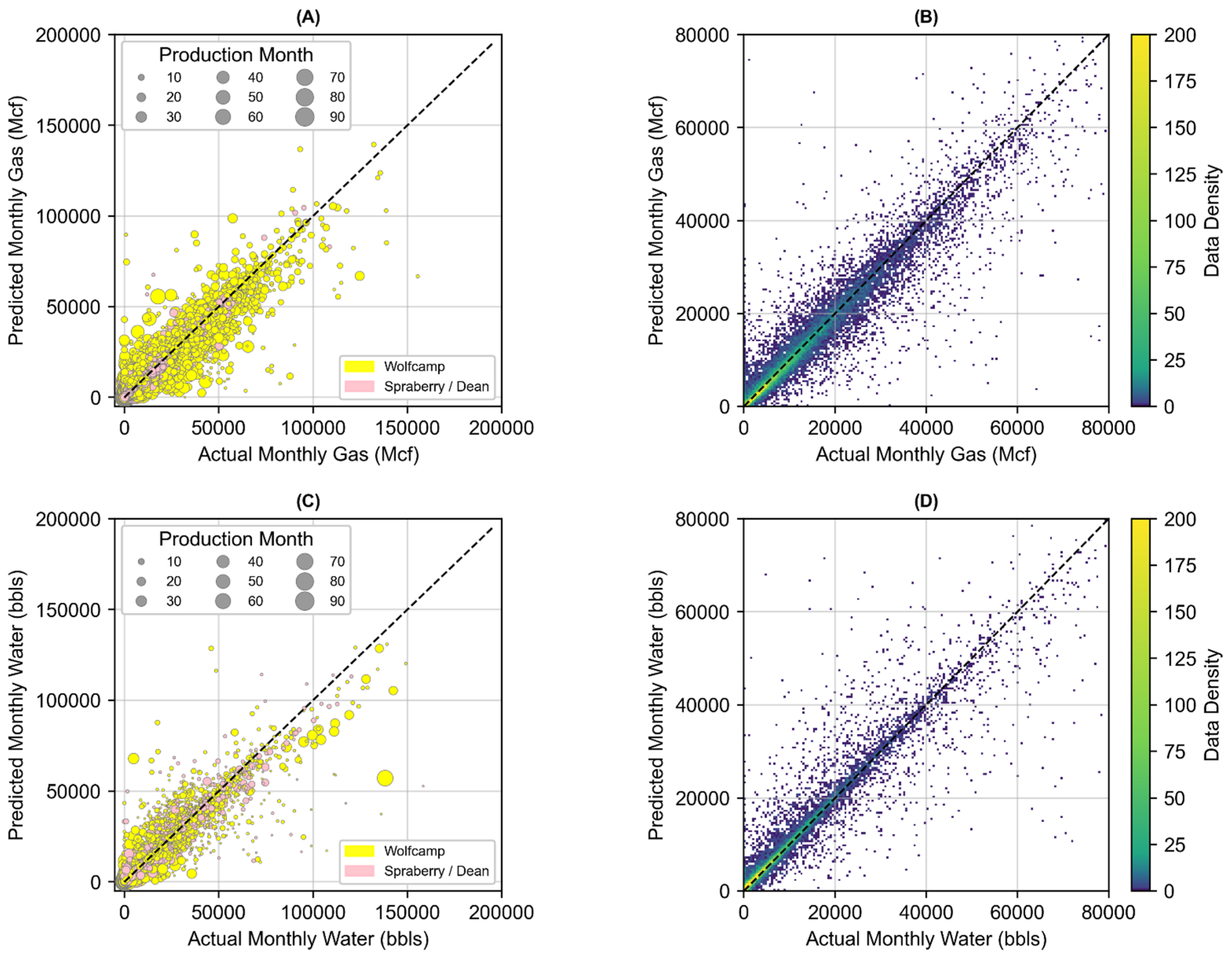
| Monthly Gas (Mcf) | 0.930 | 7.63 × 10⁶ | 2762 | 0.931 | 7.54 × 10⁶ | 2746 |
| Monthly Water (bbls) | 0.914 | 6.72 × 10⁶ | 2593 | 0.899 | 7.35 × 10⁶ | 2710 |
| Joint Prediction (Monthly Water and Gas) | 0.922 | 7.17 × 10⁶ | 2679 | 0.915 | 7.44 × 10⁶ | 2728 |
| Response Feature | Outlook Year | Midland Basin Well Cluster Number: 0 through 8 | ||||||||
| 0 | 1 | 2 | 3 | 4 | 5 | 6 | 7 | 8 | ||
| Cumulative Oil (Mbbls) | 1st year | 77 | 111 | 147 | 100 | 38 | 181 | 86 | 82 | 73 |
| 5-years | 154 | 282 | 275 | 183 | 74 | 346 | 156 | 169 | 145 | |
| Cumulative Gas (Bcf) | 1st year | 0.16 | 0.20 | 0.25 | 0.15 | 0.12 | 0.27 | 0.25 | 0.13 | 0.22 |
| 5-years | 0.29 | 0.58 | 0.62 | 0.23 | 0.23 | 0.60 | 0.76 | 0.21 | 0.79 | |
| Cumulative Water (Mbbls) | 1st year | 154 | 230 | 268 | 181 | 102 | 304 | 200 | 162 | 182 |
| 5-years | 289 | 587 | 545 | 347 | 175 | 659 | 358 | 324 | 328 | |
| Response Feature | Outlook Year | Midland Basin Well Cluster Number: 9 through 17 | ||||||||
| 9 | 10 | 11 | 12 | 13 | 14 | 15 | 16 | 17 | ||
| Cumulative Oil (Mbbls) | 1st year | 141 | 89 | 80 | 87 | 160 | 135 | 129 | 237 | 50 |
| 5-years | 281 | 173 | 168 | 167 | 328 | 265 | 279 | 465 | 91 | |
| Cumulative Gas (Bcf) | 1st year | 0.26 | 0.14 | 0.12 | 0.15 | 0.31 | 0.22 | 0.22 | 0.34 | 0.12 |
| 5-years | 0.57 | 0.19 | 0.16 | 0.27 | 0.91 | 0.50 | 0.45 | 0.85 | 0.27 | |
| Cumulative Water (Mbbls) | 1st year | 271 | 185 | 170 | 171 | 306 | 249 | 265 | 373 | 111 |
| 5-years | 574 | 364 | 287 | 332 | 684 | 515 | 621 | 879 | 178 | |
| Metric | Oil Production | Natural Gas Production | Water Production | Gas-to-Oil | Water-to-Oil | |||||
|---|---|---|---|---|---|---|---|---|---|---|
| Mbbls | Cluster | Bcf | Cluster | Mbbls | Cluster | Bcf/Mbbl | Cluster | Mbbl/Mbbl | Cluster | |
| Highest 1st year | 237 | 16 | 0.34 | 16 | 377 | 16 | 0.0014 | 16 | 1.59 | 16 |
| Highest 5 years | 465 | 16 | 0.91 | 13 | 879 | 16 | 0.0020 | 11 | 1.89 | 11 |
| Lowest 1st year | 38 | 4 | 0.12 | 4 and 11 | 102 | 4 | 0.0032 | 4 | 2.68 | 4 |
| Lowest 5 years | 74 | 4 | 0.16 | 11 | 175 | 4 | 0.0022 | 8 | 2.36 | 4 |
Publisher’s Note: MDPI stays neutral with regard to jurisdictional claims in published maps and institutional affiliations. |
© 2022 by the authors. Licensee MDPI, Basel, Switzerland. This article is an open access article distributed under the terms and conditions of the Creative Commons Attribution (CC BY) license (https://creativecommons.org/licenses/by/4.0/).
Share and Cite
Vikara, D.; Khanna, V. Application of a Deep Learning Network for Joint Prediction of Associated Fluid Production in Unconventional Hydrocarbon Development. Processes 2022, 10, 740. https://doi.org/10.3390/pr10040740
Vikara D, Khanna V. Application of a Deep Learning Network for Joint Prediction of Associated Fluid Production in Unconventional Hydrocarbon Development. Processes. 2022; 10(4):740. https://doi.org/10.3390/pr10040740
Chicago/Turabian StyleVikara, Derek, and Vikas Khanna. 2022. "Application of a Deep Learning Network for Joint Prediction of Associated Fluid Production in Unconventional Hydrocarbon Development" Processes 10, no. 4: 740. https://doi.org/10.3390/pr10040740
APA StyleVikara, D., & Khanna, V. (2022). Application of a Deep Learning Network for Joint Prediction of Associated Fluid Production in Unconventional Hydrocarbon Development. Processes, 10(4), 740. https://doi.org/10.3390/pr10040740