Article

Application of a Deep Learning Network for Joint Prediction of Associated Fluid Production in Unconventional Hydrocarbon Development

1
Department of Civil and Environmental Engineering, University of Pittsburgh, Pittsburgh, PA 15261, USA
2
Department of Chemical and Petroleum Engineering, University of Pittsburgh, Pittsburgh, PA 15261, USA
*
Author to whom correspondence should be addressed.
Processes 2022, 10(4), 740; https://doi.org/10.3390/pr10040740
Submission received: 6 March 2022 / Revised: 30 March 2022 / Accepted: 8 April 2022 / Published: 11 April 2022
(This article belongs to the Special Issue Oil and Gas Well Engineering Measurement and Control)

Abstract

:
Machine learning (ML) approaches have risen in popularity for use in many oil and gas (O&G) applications. Time series-based predictive forecasting of hydrocarbon production using deep learning ML strategies that can generalize temporal or sequence-based information within data is fast gaining traction. The recent emphasis on hydrocarbon production provides opportunities to explore the use of deep learning ML to other facets of O&G development where dynamic, temporal dependencies exist and that also hold implications to production forecasting. This study proposes a combination of supervised and unsupervised ML approaches as part of a framework for the joint prediction of produced water and natural gas volumes associated with oil production from unconventional reservoirs in a time series fashion. The study focuses on the pay zones within the Spraberry and Wolfcamp Formations of the Midland Basin in the U.S. The joint prediction model is based on a deep neural network architecture leveraging long short-term memory (LSTM) layers. Our model has the capability to both reproduce and forecast produced water and natural gas volumes for wells at monthly resolution and has demonstrated 91 percent joint prediction accuracy to held out testing data with little disparity noted in prediction performance between the training and test datasets. Additionally, model predictions replicate water and gas production profiles to wells in the test dataset, even for circumstances that include irregularities in production trends. We apply the model in tandem with an Arps decline model to generate cumulative first and five-year estimates for oil, gas, and water production outlooks at the well and basin-levels. Production outlook totals are influenced by well completion, decline curve, and spatial and reservoir attributes. These types of model-derived outlooks can aid operators in formulating management or remedial solutions for the volumes of fluids expected from unconventional O&G development.

1. Introduction

The continued pursuit for reliable, affordable, and secure supplies of energy accentuates the necessity for continued research into ways to economically and efficiently access the vast amount of unconventional natural gas and oil resources that exist. Over the last decade and a half, the application of horizontal drilling techniques coupled with advanced, multi-stage hydraulic fracturing technologies has facilitated the widespread development of unconventional oil and gas (O&G) reservoirs (such as shale and tight oil reserves) [1], resulting in a revolution in the energy landscape [2,3,4], particularly in the United States (U.S.).
Hydraulic fracturing methods make use of injected liquids under high pressure to generate breakages in subsurface formations and are usually implemented where low permeability conditions exist. The fracturing fluid is composed of a base fluid, typically water, constituting >98 percent of the total fluid volume [5] with the remaining contribution coming from proppant and chemical additives. The goal of the hydraulic fracturing process is to promote the generation of new fractures in the tight hydrocarbon-bearing rock formations inherently low in both permeability and porosity while simultaneously augmenting the size, magnitude, and connectivity of existing fractures to stimulate oil and/or gas flow to wells [6,7,8]. Once the hydraulic fracturing process is completed, the high in situ pressures within the reservoir as compared to the lower bottomhole pressure in the wellbore (which can be managed via artificial lifting) prompts fluids to migrate towards the well and be produced at the surface. The fluid that returns to the surface may contain a combination of hydrocarbons (oil and/or gas) and water, in addition to injected chemical additives from the hydraulic fracturing process, as well as naturally occurring materials such as brines, metals, and radioactive materials [9]. Each constituent requires some form of management, depending heavily on the intended endues of each, which may include sale to market as a commodity, reuse as part of site operations, or treatment and disposal.
Horizontal wells drilled and completed in shale gas and tight oil formations make up the preponderance of hydrocarbon production in the United States. Specifically, crude oil production from tight formations alone reached 6.5 million barrels per day in the U.S. through 2018, accounting for 61 percent of the total oil produced in the U.S. The U.S. Energy Information Administration (EIA) indicates that use of horizontal wells accounted for 96 percent of the overall U.S. crude oil production from tight formations by the end of 2018 [10]. A recent surge in the development of tight oil reserves located in the Permian Basin in western Texas and eastern New Mexico (41 percent of total tight oil production in the U.S. in 2018) has led to considerable growth in overall U.S. crude oil production [11].
While unconventional oil (and gas) resources remain critically important in the pursuit towards energy security, challenges persist in effectively forecasting their production potential. For instance, productivity in unconventional reservoirs is known to be responsive to the nature and effectiveness of the interactions between wellbore design, completion and stimulation processes, and the inherent irregularities in reservoir conditions. As a result, fluid production responses can be highly disparate across: (1) An entire O&G play [12]; (2) wells on a given pad targeting the same formation; or even (3) the different perforation stages of single well’s lateral component [13]. Production forecasts hold implications on the strategic decisions made by the O&G sector. For instance, resulting production outlooks, depending on the long-term trajectories of fluid volumes produced, can prompt macro-scale consequences such as potential fluctuations in oil and/or gas market prices and associated impacts on the environment [14]. Additionally, forecasts can influence micro-scale outcomes that ultimately shape a wide range of operating and maintenance scenarios for field operators or even affect company profit margins. Reservoir modeling and simulation are commonly used to inform decision makers regarding the potential production response and long-term performance of hydraulically fractured horizontal wells in unconventional reservoirs. These approaches can be costly in terms of the time and computational resources needed to execute effectively [15,16]. Furthermore, difficulties exist in attaining sufficient levels of geological data at the well level [17] to sufficiently reflect the diversity in reservoir conditions needed to model fluid flow. This challenge intensifies when the interest spans to multi-well performance evaluation at the field-scale or larger.
Given the computational resources that are typically widely available and the emergence of O&G digital datasets that include features associated with well completion, stimulation, and production, many have taken to machine learning (ML) and data analytics as a compliment to existing approaches for O&G production analysis [18,19,20]. ML-based tactics can provide additional analytical functionality to traditional reservoir simulation methods. They have proven effective in accurately and reliably modeling circumstances involving highly complex systems where variable conditions are known to be prominent, not uncommon to wellbore/reservoir relationship interactions in unconventional O&G development. Additionally, they offer expeditious predictive capability, allowing practitioners to quickly generate multiple realizations thereby enabling greater insight into the systems modeled [21].
A number of potential use cases exist where ML has been applied as part evaluating the effects of hydraulic fracturing designs on hydrocarbon production in unconventional reservoirs. As an example, several studies utilize static productivity indicators that reflects cumulative production under a fixed time duration (i.e., six months or one year) as response variables [22,23,24,25,26] to evaluate potential well response to various hydrofracking completion designs. The use of static response variables enabled straightforward evaluation of input feature impact rating and ranking, as well as sensitivity evaluation. The findings from these studies have proven insightful in identifying key production drivers representative to the study areas evaluated, as well as effective in approximating well productivity potential given the associated completion design and placement choices. However, the findings are not directly translatable to applications in the oil and gas space requiring more dynamic, temporal-dependent considerations. Well history matching, hydrocarbon production forecasting, and facilitating data-driven production outlook scenarios are examples that come to mind [27,28,29,30].
Many studies are taking focus on using ML for dynamic reservoir analysis by evaluating time series-based topics, such as oil or gas production over the life of producing wells. These studies are leveraging empirical data that includes daily or monthly cumulative hydrocarbon production values over all or a portion of each well’s productive life. Many of the relevant studies apply deep learning ML strategies in order to capture and generalize the intrinsic temporal or time sequence-based properties within the data. Findings from recent studies indicate that the deep learning approaches applied have been exceedingly effective at predicting dynamic production trends accurately on holdout data. The results of which suggests that these approaches hold substantial implications and potential viability in production forecasting.
To gain further comprehension on O&G-related time series analysis using ML, we provide a short review of relevant studies works that have focused on this topic. A study by Jie et al. developed two deep learning models to predict daily gas production from a single well completed in the Sichuan basin in China [31]. The researchers developed artificial neural network- (ANN) based models using: (1) A fully-connected multilayer perceptron (MLP)-based ANN with a single hidden layer and (2) a long-short term memory- (LSTM) based ANN with stacked LSTM layer architecture. Empirical data for daily gas production over a three-year period was used for analysis. The first 900 dataset observations were used for model training and the last 100 observations were used for holdout model performance testing. Input data included the data features (assumed at daily resolution) of oil pressure, casing pressure, daily water production, cumulative gas production, cumulative water production, and water-gas ratio. Results indicated prediction error of 1.56 percent for the LSTM-based model and upwards of 9.66 percent for the MLP-ANN. Sagheer and Kotb implemented deep LSTM architectures to estimate monthly oil production for two oil fields; one was the Tarapur Block of Cambay Basin to the west of Cambay Gas Field in India and the other in the Huabei oilfield in China [32]. They demonstrated the predictive effectiveness in stacking LSTM layers as part of network architecture when long interval temporal dependencies may exist as compared to model performance when shallow neural network architectures are used. Additionally, the researchers noted that their LSTM-based model outperformed counterpart formulations explored that were based on deep recurrent neural networks (RNN) and Deep Gated Recurrent Unit models. The work performed by Liu et al. included the development of an ensemble empirical mode decomposition (EEMD) based LSTM learning network capable of time series forecasting of oil production. Case studies were performed using empirical field data from the SL and JD oilfields, China [33]. Their proposed EEMD-LSTM configuration outperformed other model types developed under ensembles between EEMD and MLP-based artificial neural networks and EEMD with support vector machine.
Collectively, these studies demonstrate the utility and capability of deep learning-based ML (with noted effectiveness of LSTM) for time series hydrocarbon production prediction. The knowledge gained through these works provides both a foundation as well as an opportunity to extend these approaches to other aspects critical to O&G development where: (1) Dynamic, temporal dependencies exist; (2) said aspects possess significant connotations to production forecasting; and (3) that have not been extensively explored in previous research. An obvious need that meets these criteria would be to possess the ability for assessing the potential volumes of the associated water and natural gas produced in tandem with crude oil. Many operators targeting oil-rich unconventional reservoirs are faced with the challenge of managing large volumes of water and natural gas that are often co-produced. Limited natural gas processing and pipeline takeaway capacity can force operators to resort to venting or flaring produced natural gas.
Venting is the direct release of natural gas produced from O&G operations to the atmosphere. Flaring involves the controlled combustion of produced natural gas at the wellhead, converting methane to carbon dioxide and water vapor. From an environmental standpoint, flaring is less detrimental than venting given that carbon dioxide is 25 to 28 times less potent as a greenhouse gas than methane over a 100-year period [34,35]. According to the EIA, the quantities of natural gas vented or flared from O&G wells in the U.S. reached record levels in 2019 averaging 1.48 billion cubic feet per day (Bcf/day) (1.3 percent of the total natural gas volume produced) [36]. Texas and North Dakota contributed nearly 85% (1.3 Bcf/day) of all reported flaring and/or venting (only Texas contributed to gas venting) of produced natural gas. Produced water is often managed via disposal through deep well underground injection.
The injection of large volumes of waste water from O&G operations has been strongly correlated to the increased frequency of occurrence of induced seismic events including magnitude 2+ earthquakes, particularly in Oklahoma, Ohio, Arkansas, West Virginia, and Texas [37]. Literature suggests that many are working to generate solutions and reuse options for associated gas and water production [38,39,40,41,42]—but a need exists to be able to effectively quantify and forecast produced volumes of both natural gas and water to best inform the development of management or remedial solutions as well as grasp the potential environmental implications for planned O&G development [43].
We propose a combination of supervised and unsupervised ML approaches as part of a framework that can reliably estimate both produced water volumes and natural gas associated with oil production in a time series fashion. This type of predictive modeling capability is expected to be useful towards (1) informing well operators as part of developing strategies to ensure the effective management, treatment, or potential reuse based on the volumes and quantities of produced fluids, and (2) supplementing hydrocarbon production outlooks with additional fluid volumes in time series fashion. Additionally, this work offers a novel complement to other noted O&G machine learning-based predictive models from literature; largely achieved through its joint prediction functionality, capability to either reproduce or forecast cumulative volumes of natural gas and water produced alongside oil at the well level, and its applicability centered towards a major oil and gas producing play. In addition, the ensemble of the supervised and unsupervised elements of this work enables a means to rapidly forecast oil, water, and natural gas production at the well level as influenced by operational development considerations.
The focus of this study is on the Permian Basin region of the U.S. The region holds enormous consequence regarding domestic oil and gas production. According to a report by the Texas Independent Producers & Royalty Owners Association, yearly crude oil production in the Permian Basin has grown by 1.2 billion barrels since 2009, resulting in a 371% increase in oil output over the last ten years [44]. This overall growth has enabled the Permian to become the world’s top-producing oil field [45]. While the region itself is a major producer of both oil and gas, the basin currently faces several challenges. These include: (1) Steeper well decline rates and lower initial production (IP) values as development is moving to non-core regions; (2) associated natural gas production has outpaced pipeline takeaway capacity, which has led to an increase in flaring and venting practices; and (3) produced water volumes and associated management costs are both on the rise [43,46,47]. Combined, these impacts threaten to potentially lower the Permian’s overall production potential while consequently increasing the environmental burden associated with O&G operations. Therefore, an opportunity exists to propose research targeted towards these specific challenges and would provide beneficial outcomes to both potentially improving recovery and estimation of the types and volumes of fluids produced at the well level—each of which require specific management strategies and bear potential environmental implications.

2. Data and Methods

The focus of this study is to generate a ML-based prediction model capable of time series joint prediction of associated natural gas and water that are produced alongside oil as part of unconventional hydrocarbon development (three-stream production example presented in Figure 1). Secondarily, this study aims to demonstrate the utility of such a model as a compliment to existing O&G operational management strategies.
The model is based on a deep neural network architecture leveraging LSTM layers in order to accommodate time-dependent conditions in the data and be proficient towards multi-output prediction. The model development workflow, described throughout the following subsections, is interconnected with several data preprocessing steps that includes data sub-division, engineering of new features, outlier removal, data standardization, and feature selection. The model would have the functionality to not only replicate well production history (the primary focus of many existing time series O&G analyses), but also enable forward-based fluid production forecasts for existing wells throughout their remaining productive lives, as well as be used to predict fluid volumes in time series fashion at new (i.e., theoretical) well sites where no historic production data exists. Additionally, the ML-based model proposed here is intended to be applicable across multiple producing reservoirs, focusing on the “Wolfberry” pay zones (highlighted in Upper Spraberry through Cisco/Cline [Wolfcamp D] reservoirs in Table 1). Such a model will help provide a data-driven approach for a more holistic evaluation towards field development where multiple producing reservoir options are co-located. The volatility that exists in oil and gas market prices and supply and demand encourages operators to remain informed to the best extent possible of potential risks and opportunities they may face over both the short and long term [49]. The inherent challenges facing the Permian suggests that field development decision making is complex. Overall, this study proposes a modeling tool that works towards helping inform complex field decision choices by scaling up model outputs via a single predictive model.

2.1. Study Area

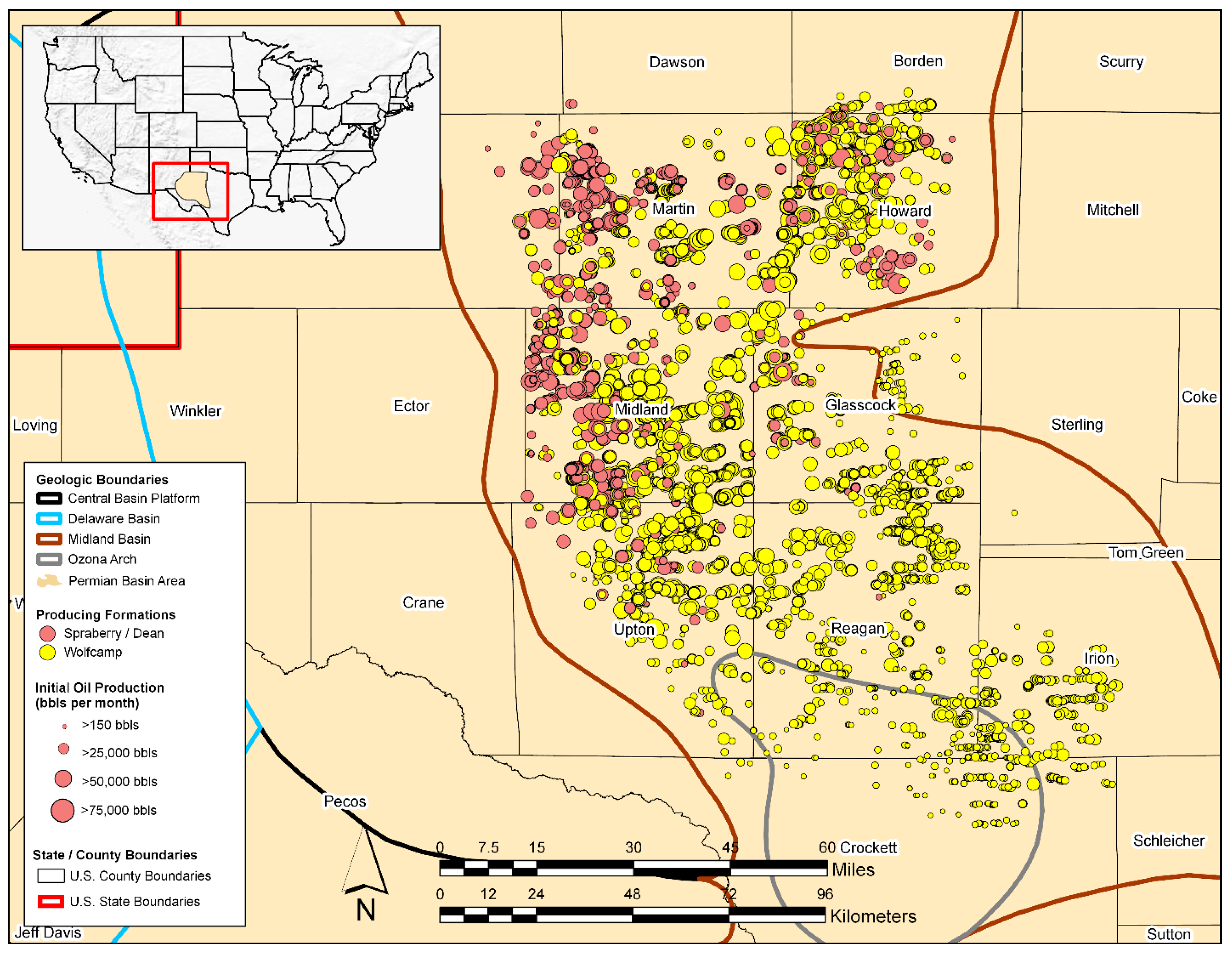
The study area for this work focuses on the Midland Basin, one of the major sub-basins of the larger Permian Basin. The Permian Basin (Permian) is an extensive sedimentary basin and major O&G-producing region geographically located in West Texas and the neighboring areas of southeastern New Mexico. The Permian spans roughly 75,000 square miles and comprises greater than 7000 fields in West Texas alone [50]. The Permian has been important in the U.S. energy economy for nearly a century. According to the EIA, the Permian has produced hydrocarbons for approximately 100 years and has supplied more than 35.6 billion barrels of oil and roughly 125 trillion cubic feet of natural gas (data as of January 2020). The Permian accounted for approximately 35 percent of the total U.S. crude oil production and over 13% of the total U.S. natural gas production in 2019 [51]. It is expected to remain one of the largest hydrocarbon-producing regions in the world with remaining reserves on the order of 46 trillion cubic feet of natural gas and over 11 billion barrels of oil [52]. The Permian contains several sub-basins and platforms that include the westernmost Delaware Basin, Central Basin Platform, and the easternmost Midland Basin [53]. The extent of the Central Platform and Midland sub-basins as well as the eastern edge of the Delaware Basin is shown in Figure 2.
The Midland Basin is the eastern subbasin of the larger Permian Basin and is bordered by carbonate platforms such as the Central Basin Platform, Eastern shelf, and Northern shelf. The basin is at its deepest on its western edge and shallows to the east. Towards its southernmost portion, basin’s formations start to thin towards the Ozona Arch—an extension of the Central Basin Platform [53]. The stratigraphy within the Midland Basin is characterized as containing several stacked geologic sequences that offer hydrocarbon producing potential. Two stratigraphic sections within portions of the Leonardian and Wolfcampian epochs that have been a focus of substantial O&G development are the Spraberry (along with the Dean) and the Wolfcamp formations; collectively referred as the “Wolfberry” [54] (Table 1). The stratigraphic groupings that make up the Wolfberry series of reservoirs serve as the primary producing pay zones of interest evaluated in this study.
Table 1. Stratigraphic description for a subset of the Midland Basin, Texas. The producing reservoirs of interest to this study are highlighted (Spraberry in pink and Wolfcamp in yellow). This figure was generated from collective content compiled from lithostratigraphic interpretations of the Permian Basin from several literature sources [51,53,55,56,57,58,59,60].
EraPeriodEpochLocal
Series
Stratigraphic/Formation NameReservoir Operational Name
PaleozoicPermianGuadalupianWardSan AndreasSan Andreas
San Angelo/GlorietaSan Angelo/
Glorieta
LeonardianClearforkUpper Leonard
WichitaUpper SpraberrySpraberry
Lower Spraberry
Dean
Lower LeonardWolfcampWolfcamp A
WolfcampianWolfcampWolfcamp B
Wolfcamp C
PennsylvanianVirgilianCisco/ClineWolfcamp D
MissourianCanyonCanyon
Des MoinesianStrawnStrawn
AtokanAtoka/BendAtoka/Bend
The Lower Permian aged (Leonardian epoch) Spraberry and Dean formations are made up of interbedded turbidite sands, laminated siltstone, carbonate, and organic-rich shales [57]. The Spraberry consists of upper- and lower-unit intervals [61,62] (certain interpretations include a middle Sprayberry and Jo Mill as well [63,64])—the Dean formation is located stratigraphically beneath the Lower Spraberry. Each stratigraphic unit is distinguished by its lithologic composition. For instance, each of the three formations consists of thick sequences of fine-grained sandstones and siltstones that lie on top of an equally thick lower unit made up of black shales and dark carbonates [65]. The formations are known to be generally under-pressured (averaging 800–900 psi [5.4–6.1 MPa]) with matrix porosity ranging from 6 to 15 percent, matrix permeability below 10 md, and are highly naturally fractured [54,66,67]. The average true vertical depth to the top of the Upper Spraberry unit is roughly 6800 feet across the Midland Basin. The complete section from the top of the Upper Spraberry to the base of the Dean ranges in thickness between 1200 and 1870 feet [54]. Similar to other unconventional hydrocarbon plays, productivity in the Spraberry fluctuates across the basin [68].
The early Permian aged (Wolfcampian-Leonardian epoch) Wolfcamp is described as a mixed siliciclastic-carbonate succession with stacked stratigraphic units comprising of cyclic gravity flow deposits—each separated by mudstone and siltstone [51]. The Wolfcamp is described by Sutton [54] as a dual-lithology system consisting of organic-rich shale with interbedded limestone. Lower reservoir quality portions of the Wolfcamp are associated with the presence of grainy carbonate facies, whereas higher reservoir quality portions have been tied to the occurrence of siliceous mudstones [69]. The entire section of the Wolfcamp ranges in porosity between 2 and 12 percent with average permeability near 10 millidarcies (mD) [51]. The formation varies substantially across the Midland Basin in terms of depth, thickness, and lithologic composition. The Wolfcamp is at its deepest near the center of the Midland Basin, measuring approximately 12,000 feet deep. It shallows substantially towards the edges of the basin, varying in depth from 4000 to 7000 feet [54]. The thickness of the entire section of the Wolfcamp averages around 1800 feet. The Wolfcamp is extensive throughout the Permian Basin and is considered one of the most abundant unconventional O&G plays worldwide. The Wolfcamp formation has been appealing to O&G operators given its stacked configuration, in which multiple thick hydrocarbon-producing zones exist in sequence [70]. The stacked intervals of the Wolfcamp formation are called benches—from shallow to deep they are referred to as A, B, C, and D. Each bench has shown to be different in terms of its overall lithology, fossil content, total organic carbon content, and thermal maturity [71]. Saller et al. (1994), Blomquist (2016), and Peng et al. (2020) provide detail on the geologic composition of the Wolfcamp and various benches within and therefore the differentiation is not described at length here [72,73,74]. Recent development efforts in the Midland Basin are preferentially targeting the more oil-rich Wolfcamp A and B (roughly 95 percent of total Wolfcamp production) opposed to the more gas-rich Wolfcamp benches C and D [71,75].
Figure 2. Map of the study area in the Midland Basin, Texas. Well data used for the study was acquired from DrillingInfo/Enverus [76]. The geographic information system (GIS) layers applied to support the generation of this figure were acquired from the University of Texas at Austin [77] and United States Geological Survey [78].
Processes 10 00740 g002
The Permian region and associated sub-basins have been known to produce large volumes of natural gas and water that are co-produced with oil. A study by Kondash et al. has noted that Permian Basin wells have increased the water used per well as part of hydraulic fracturing operations from 30,800 barrels per well in 2011 up to 267,325 barrels per well in 2016—a 770 percent increase [79]. The flowback and produced water volumes during that same timespan had increased over 400 percent; averaging 56,610 barrels per well in 2011 to over 232,700 barrels per well in 2016. Specifically, in the Midland Basin, waste water disposal volumes derived from O&G operations have steadily increased since 2011, reaching approximately 4.5 billion barrels per day in 2017 [80].
In 2017, flaring and venting of natural gas in the Permian basin in Texas and New Mexico was estimated at nearly 300 million cubic feet per day (MMcfd), roughly 4.4 percent of the total gas produced that year. In that same year, the Midland Basin produced approximately 1019 billion cubic feet (Bcf) of natural gas, and flared 24 Bcf of that total (2.35 percent of all gas produced) [81]. In 2019, flaring and venting of natural gas in the Permian reached an all-time record high based on the year’s third quarter estimates, averaging 752 MMcfd (275 Bcf total) [82]. The Midland Basin portion of 2019 flaring ranged from approximately 150 to 290 MMcfd [83].
Well data leveraged for this study (described further in Section 2.2) are grouped based on the associated targeted producing reservoirs listed in Table 1. Wells are tabbed as either “Spraberry/Dean” or “Wolfcamp” dependent upon their associated Stratigraphic/Formation Name. The wells used as part of this study are plotted in Figure 2; they are colored based on their associated producing formation and sized based on each well’s initial oil production (in barrels [bbls]/month).

2.2. Study Data Overview and Data Processing

Much of the well completion and production-related data used for this study is acquired from the O&G data vendor DrillingInfo/Enverus [76]. Other features were derived through feature engineering to further supplement the available feature dataset. The dataset contains features related to well production performance attributes, Arps decline curve attributes [84], well completion attributes, and spatial and reservoir attributes—all specific to horizontal production wells spanning the Spraberry/Dean and Wolfcamp producing intervals (highlighted in Table 1) in the Midland Basin with drilling initiation dates within the 1 January 2010 to 30 June 2020 timeframe. The dataset includes a combination of static (well data that does not change over the well’s productive lifetime) and dynamic features (well data with temporal dependencies—mostly three-stream production data) for the wells meeting these screening criteria. This database query yields data for approximately 6480 wells in total in which each well has data reported for all features of interest (both static and dynamic features) and duplicate entries are omitted. No attempts at data interpolation with respect to missing values occurs in this study.
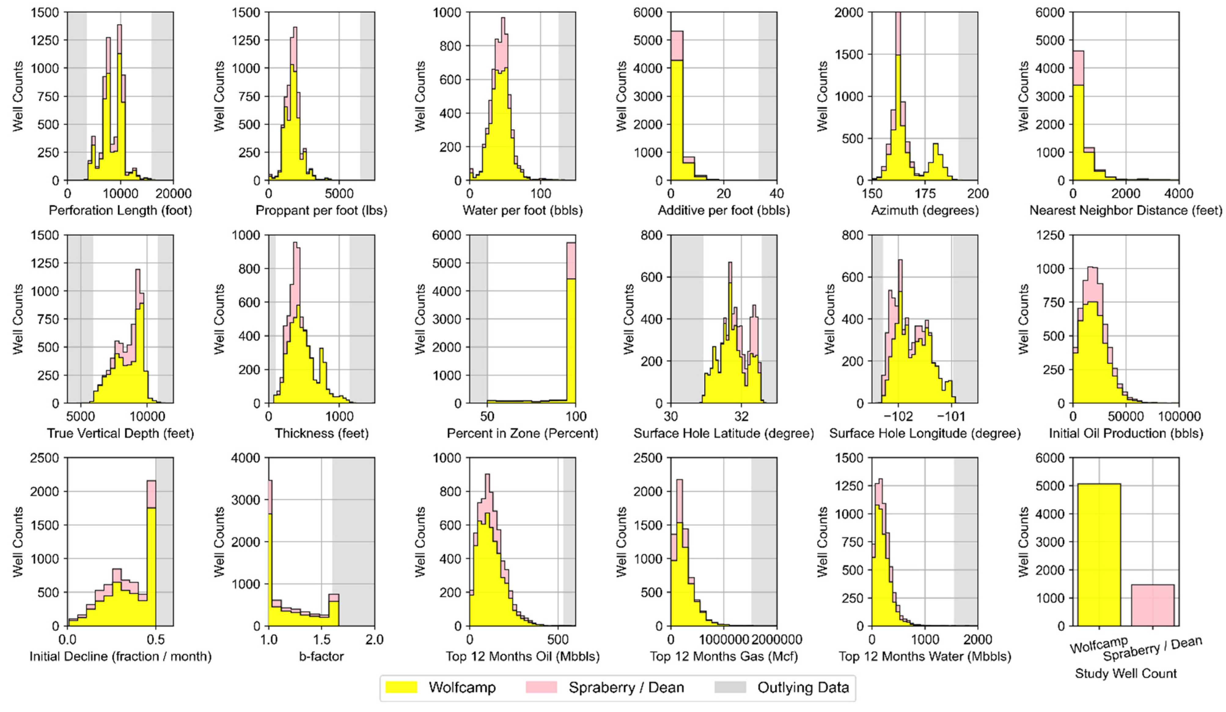
The distributions of the static study features of interest are evaluated to screen and remove potential outlying well data and refine the overall dataset. Their distributions are presented in Figure 3. Data outside of +/− 3 standard deviations from a given feature’s mean value (grey margins within subplots in Figure 3) are considered outlying and possibly highly influential on ML model response [85,86]; even if distributions are not explicitly gaussian. All outlying data is removed from the static and dynamic contributions to the dataset (approximately 270 wells had features meeting outlying criteria). The resulting dataset consists of 6210 wells in total extending across 12 Texas counties, the extent of which is plotted in Figure 2 and the descriptive statistics for features from these wells are summarized in Table 2.
The features within each data group from Table 2 have a specific role as part of the hydraulic fracturing and oil/gas production process. The breadth of data features available within the study dataset affords the opportunity to explore a multitude of aspects related to unconventional oil and gas production in the Midland Basin. Data groupings and their associated features are briefly described next.
  • Well Performance Attributes: These features relate to fluid production for wells in the study dataset. The dynamic features within the data group represent summation of the three-stream (oil, gas, and water) empirically-derived monthly values at the well level provided by DrillingInfo/Enverus. Data for these dynamic features is available for each month in a given well’s productive lifetime. Therefore, the volume of this data varies across wells depending on when they began production and how long wells are kept online. The “Top 12-months” static features for oil, gas, and water were derived via summation of the 12 largest observed values for each well based on monthly dynamic feature data. This approach has been implemented in our prior work [12,23] and has proven to effectively represent productivity potential for unconventional wells that may or may not have been subject to disruptions to their production time series profiles. Both the Top 12-months Oil and Gas features correlate strongly to well level estimated ultimate recover (EUR) as indicated in Figure 4. The static EUR features represent an estimation of the technically recoverable reserves at the well level. They are calculated by DrillingInfo/Enverus [87] using a combination of historic production data and a combination of Arps decline curve models [84].
  • Decline Curve Attributes: These features are inherent to decline curve analyses based on the Arps decline curve model [84]. The Arps model can be used to evaluate oil and/or gas declining production rates over time. Time-dependent reduction in hydrocarbon production can be attributed to reduced reservoir pressure as well as the relative change in the volumes of the produced fluids. The approach can also be used to forecast hydrocarbon production into the future. The Arps approach is based on fitting a mathematical decline model (either exponential, hyperbolic, or harmonic) to empirical observations of an asset’s (i.e., well) performance history [88]. Well features related to initial (oil) production, the initial decline, and degree of curvature (b-factor) are the parameters related to the Arps model. Values for these features for each well in the study dataset have been determined by Drillinginfo/Enverus [87]. The DrillingInfo/Enverus approach solves for the most appropriate Arps model parameters that minimize the sum of squared errors based on empirical production values for a given well [87]. DrillingInfo/Enverus restricts b-factors between 0 and 2. The b-factor is typically greater than 1 in unconventional shale plays given the inherent low permeability rock matrix and resulting extended duration of transient flow [89]; potentially a derivative of the bulk of empirical observations with shorter producing timeframes [90].
  • Well Completion Attributes: These features pertain to each well’s design and completion attributes as it relates to well placement, orientation, and hydraulic fracturing design. The major hydraulic fracturing design features include the length of the perforated interval contacting the reservoir and the volume of proppant, water, and additive used for hydraulic fracturing normalized to a per foot of perforated interval basis. Proppant includes solids that may vary in size, shape or material type. They typically consist of sand or engineered materials (i.e., resin-coated sand or high-strength ceramic materials such as sintered bauxite) and are used to keep reservoir fractures open and conductive following hydraulic fracturing [91]. Additives may serve a variety of functions, with examples including the assurance of effective transport of water and proppant downhole and throughout the reservoir, as well as to ensure sustained hydrocarbon recovery after hydraulic fracturing. Specific components can tend to vary from one well to another and from operator to operator. However, example constituents include acids, friction reducers, biocides, pH adjusters, scale inhibitors, iron stabilizers, corrosion reducers, gelling agents, and cross-linking agents [92,93]. Other important well design characteristics captured in the dataset relate to the wellbore lateral orientation, spacing distance to nearby wells, and the portion of the horizontal perforated length within the targeted producing reservoir zone of interest. The directional alignment (reflected by azimuth) is often a design choice by field operators; one that is driven by the natural orientation of in situ stresses in targeted reservoir producing zones. Horizontal segments of wells that are drilled along the minimum horizontal stress often produce transverse fractures following horizontal fracturing. This form of fracturing may improve drainage efficiency. As a result, well laterals oriented properly on azimuth given natural in situ stress regimes may experience higher productivity [5,92]. Well azimuth was approximated based on the geographic orientation between each well’s surface hole latitude and longitude and lateral toe latitude and longitude. Well spacing may provide insight into the field operator’s anticipated drainage area based on the applied water and proppant intensity. Additionally, spacing-related data can be helpful in determining if closely-spaced wells suffer from possible interference from hydraulic fracturing operations (i.e., frack hits) or effects from parent/child well interactions [94,95] from nearby wells. We approximated the nearest well distance for each well in the dataset using the haversine formula and bottom hole latitude and longitude coordinates to its closest well neighbor prior to any dataset reduction. Percentage in zone is a metric which provides an indication of the wellbore geo-steering efficiency of the horizontal lateral component. DrillingInfo/Enverus provides this data readily for each well. Wells with a high portion of their perforated segment in the targeted producing zone are more likely to be better producers than those wells expected to deviate substantially off target. Each feature in this data group is treated as static. In actuality, many of these features, such as proppant, water, and additive per foot, could essentially vary over the life of any given well due to refracturing campaigns.
  • Spatial and Reservoir Attributes: The features included attempt to best approximate the variability that may exist in the geologic conditions which influence hydrocarbon prominence and producibility that span the reservoirs of interest across the study domain. True vertical depth and thickness (i.e., reservoir thickness) are provided from DillingInfo/Enverus for each well. However, other relevant geologic characteristics that are known to influence hydrocarbon production, such as total organic carbon, porosity, hydrocarbon and/or water saturation, thermal maturity, reservoir pressure, existence of fracture networks, and capacity of the reservoir(s) to be hydraulically fractured [96,97,98,99], are not directly or readily available in bulk. Additionally, many of these features are dynamic in nature and change over the duration of hydrocarbon production (such as fluid saturation and pressure in the reservoir), while others essentially remain static (such as porosity and thermal maturity) [100]. Each well’s locational data (surface latitude and longitude) is used as a contingency means to approximate geologic conditional variability known to vary spatially across the study area—an approach widely used in other ML-based model development efforts occurring over large spatial horizons [22,26,27,101].
Figure 4. Pearson correlation matrix for the static dataset features evaluated.
Processes 10 00740 g004
A correlation matrix using Pearson’s Product-Moment Correlation is presented in Figure 4 which provides quantitative indication of the linear relationship between each of the various static features of interest. The analysis represented in Figure 4 is informative specifically due to the fact that: (1) it suggests how attributes correspond to other attributes, as well as with potential model outputs; and (2) it serves as a diagnostic check on data quality to ensure data features are related in a fashion that is intuitive and confirmatory based on heuristic understanding of the Midland Basin.
The Pearson correlations alone highlight a number of noteworthy trends. For instance, Figure 4 shows several positive relationships between many of the well performance attributes representing fluid production with well completion attributes specific to hydraulic fracturing design. The attributes of top 12-month oil, water, and gas, as well as the estimated EUR per well for both oil and gas are all positively correlated with increasing values of perforation length, proppant, and water per foot. These relationships suggest greater production results from well completion and hydraulic fracturing design upscaling; a concept noted by others [22,23,24]. Additionally, the decline curve attributes show correlation to both the well performance and well completion attribute features. Initial oil production is mostly positively correlated to these attributes, while initial decline (for oil), as expected is negatively correlated. The b-factor component is mostly uncorrelated to all features in the dataset with the exception of a positive correlation to oil EUR, and therefore holds influence over a well’s longer-term productive profile. Finally, worth noting are the correlations associated with reservoir thickness and true vertical depth based on well location in the basin. Moving west to east in the basin (based on surface hole latitude), Figure 4 suggests the reservoirs become both shallower and thinner. In contrast, reservoirs trend thicker and deeper when moving south to north (based on surface hole longitude). These correlations are as expected based on interpretations of Midland Basin reservoir depth and thickness isopaches and interpretations generated by the EIA [53,102], Hamlin and Baumgardner [61], and Blomquist [74]. Based on this analysis, the dataset following outliers removed appears representative and suitable for use in ML model development.

2.3. Data Preprocessing Prior to Model Training and Testing

An important data preprocessing step is applied that scales attribute data to consistent ranges in order to (1) afford equal consideration to all attributes, (2) improve training efficiency and, (3) increase numerical stability of the resulting models [103]. The data scaling approach was implemented to both the static and time series parameters prior to use in the following feature selection and ML model development steps (described in Section 2.4 and Section 2.5). For the feature selection and clustering, input and response features were standardized to Z-values (Z) per Equation (1). For model training regarding the time series joint associated fluid production model, all features were scaled (i.e., normalized in this case) between 0 and 1 using linear mapping via Equation (2):
Z = x μ σ
x n o r m a l i z e d = x m i n x m a x x m i n x
where x represents feature values, μ is the feature mean value, σ is the feature standard deviation, and minx and maxx represent the respective minimum and maximum values for each dataset feature. The Z-score standardization step in Equation (1) rescales data for each parameter to a standard normal distribution with a mean of 0 and a standard deviation of 1. The data transformation from Equation (2) is used as a variant to the zero mean, unit variance standardization from Equation (1). The authors have gleaned from recent experience the effectiveness of 0 to 1 scaling in deep learning ML applications [104,105,106,107] and are therefore applied it here. Predictions using finalized ML models are rescaled to their normal unit ranges.
Following data standardization and/or normalization, project dataset features were apportioned and merged into distinct dataset aggregates for use dependent upon the machine learning model workflow they would be applied against. The workflows include feature selection (Section 2.4), clustering (Section 2.5.1), or joint time series prediction (Section 2.5.2). Each workflow utilized a distinct aggregate of the full project dataset. However, the data features that were carried forward to each framework were largely dependent on the results from the feature selection, described in Section 2.4.

2.4. Feature Selection Approach

Features (i.e., variables) that are strongly correlated are therefore linearly dependent and may have almost correspondingly similar (if positively correlated) or opposing (if negatively correlated) effects on dependent variables of interest. The Pearson correlation metric (presented in Figure 4) is limited to assessing linear relationships concerning two features. However, important functional relationships between two or more features may exist which may not be linear in nature. This can be true even if Pearson correlation coefficients are close or equal to 0 [108].
Feature selection involves a systematic process to down-select a subset of the most relevant features within the study dataset that strongly contribute to the ML model prediction response. Utilizing fewer features (and eliminating redundant or non-informative features) enables ML algorithms to train faster and more efficiently as well as decreases the likelihood of ML algorithms overfitting to irrelevant input features [109]. This study utilized recursive feature elimination with cross validation (RFECV) as a feature selection approach. The objective was to establish a final set of input features from the variety available per Table 2 that would be commonly applied as part of both the clustering evaluation and the development of the time series joint associated fluid production model.
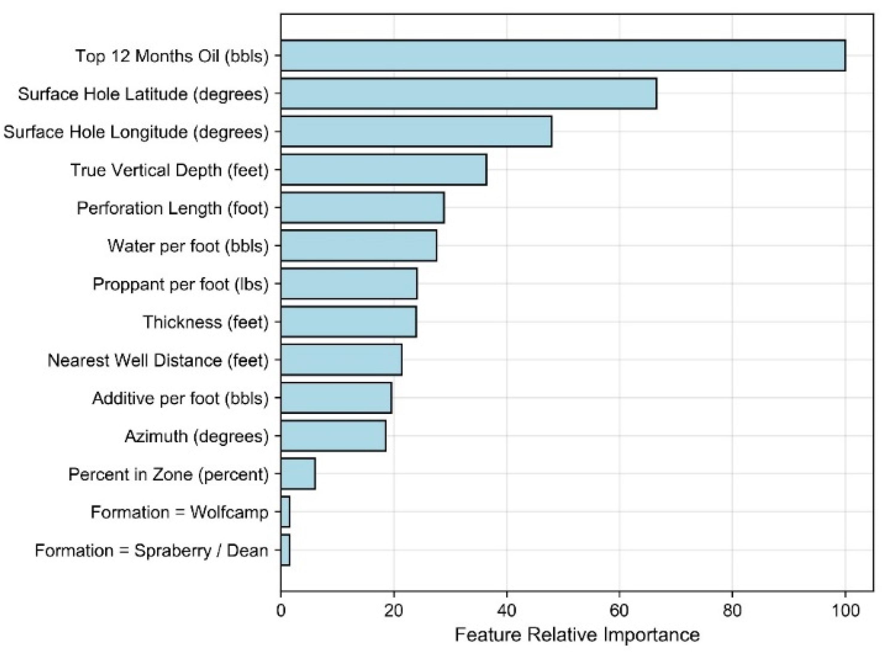
The feature elimination component of the RFECV process searches for a subset of features by starting with all features in the training dataset and fitting a ML algorithm which is used as the estimator [109,110]. The estimator is trained on the original set of features considered. A total of 14 input features (i.e., x data) are included in this study which comprise variables associated with the “Well Completion Attributes”, the “Spatial and Reservoir Attributes”, and the Top 12-months Oil listed in Table 2, as well as two categorical variables that label the production wells evaluated based on their producing reservoir group—either the Wolfcamp or Spraberry/Dean formations. Two features were used as responses (i.e., y data) which comprise of the Top 12-month Water and Top 12-Month Gas. Static data (e.g., Top 12-month Water or Gas) was used exclusively as part of the RFECV instead of dynamic time series data (e.g., Monthly Water) in order to enable more efficient training of the estimator model. The importance of each feature is acquired following model training. The feature(s) with the lowest importance are then pruned from original set of features [111,112]. The procedure is recursively repeated on the pruned set and resulting model accuracy is calculated for each iteration—the process continues until a single feature remains. The desired number of features can then be established [112,113]; typically set at the number of features that maximizes model performance, or where the inclusion of additional features does not substantially improve model performance.
Random forest (RF) was used as the estimator in the RFECV process for this study. RF-based models are considered advantageous in RFECV [114], most notably since they possess the ability to measure the importance of each feature [115] based on mean decrease impurity (described effectively by Hur et al. [116]). Prior to use in RFECV, the RF estimator’s hyperparameters were tuned via k-fold cross-validation using five folds. In this process, four folds of the training dataset are amassed to train models, and the remaining fifth fold was used to test (i.e., validate) the performance of resulting prediction models. The step was repeated so that each fold was ultimately used once for model validation while the other k − 1 folds constitute the training set [117]. An exhaustive grid search occurs as part of the cross-validation loop to tune hyperparameters. The RF estimator formulated on all 14 input data features is built on four folds training data for distinctive hyperparameter combinations evaluated [118] as part of the grid search. Trained models were then used to make predictions against held out fifth fold validation data. The process is repeated for each combination of hyperparameters evaluated. The RF-specific hyperparameters tuned as part of cross-validation includes (1) the number of trees in each forest ensemble and (2) the minimum number of samples needed to split an internal node. The maximum depth corresponding to each tree (i.e., limits the number of nodes in each tree) was unbounded. The RF hyperparameter combination that provided for the best prediction accuracy while avoiding over or underfitting was used for RFECV.
The RFECV process also involved k-fold cross-validation using five folds. For each of the five RFECV fold iterations, 14 RF models were generated with the feature subset size decreasing from 14 to 1. Resulting prediction model performance was evaluated by explained variance per Equation (3) which can effectively evaluate the multi-output response nature of the RF estimator.
explained_ variance ( y , y ^ ) = 1 V a r { y y ^ } V a r { y }
where y ^ is the predicted value, y is the observed value, and Var is the variance (or square of the standard deviation). The selected feature set from this process was then utilized as the input features for performing the clustering analysis as well as for the time series-based joint associated fluid production model. The results from RFECV is then used to inform the feature sets used for both the clustering and time series machine learning steps of this study (described in Section 2.5.1 and Section 2.5.2 respectively).

2.5. Machine Learning Model Development and Evaluation

This section describes the various ML approaches implemented as part of this study, the contribution of each towards the study objectives, and how their performance accuracy was quantified. The ML approaches utilized included both supervised and unsupervised methods, as well as the use of deep learning. Static data features that remained following RFECV step were incorporated in ML-based workflows. Python (version 3) and packages within the scikit-learn library [119] and Keras [120] were leveraged as part of the ML workflow implementation.

2.5.1. Clustering Evaluation

The majority of the static features within the study dataset underwent evaluation via k-means clustering [121], an unsupervised ML approach, prior to the development of the joint associated fluid production model. This step was intended to identify congregations of closely related wells based on their well completion, decline, well performance, and spatial and reservoir attributes (Table 2). The goal of this step was to be able to harvest Arps Decline properties (b-factor, initial production, and initial decline discussed previously) and well completion attributes representative of given clusters; from which oil production forecasts can be generated at the well level.
The k-means clustering process determines an optimal number of clusters based on the input dataset features incorporated. Assuming dataset A of V-dimensional entities aiA, for i = 1, 2, …, N, with N being the number of data entities in the dataset, k-means creates K number non-empty separate clusters S = {S1, S2, …, SK} proximal to centroids C = {c1, c2, …, cK}, by iteratively minimizing the sum of the within-cluster sum of squared distances (WK, show in Equation (4)) between each centroid and the data entities associated [122].
W K = W ( S , C ) = k = 1 K i S k d ( a i , c k )
The term d(ai, ck) in (4) is the distance between data entity ai and the associated centroid location ck. In this study, k-means analysis was performed over a wide arbitrary range of values set to K = 1 through 30 to ensure sufficient volumes of clusters are evaluated to determine an optimal.
Two heuristic algorithms were applied to determine the optimal number of clusters—the Elbow method [123] and Hartigan’s Rule [124]. The Elbow method can be used to visually evaluate Wk as a function of the number of clusters. The optimal number of clusters occurs at the point in which adding another cluster does not result in a substantial improvement to Wk. However, determining the optimal number of clusters through a visual determination approach such as the Elbow Method can be highly subjective to the evaluator’s judgement. Hartigan’s Rule provides an alternative cluster determination approach and is based on comparing the resulting Hartigan’s Index, which is a ratio between the Euclidean within-cluster sum of squared error based on k number of clusters (i.e., Wk) to that based on k + 1 clusters (Wk+1). The rule utilizes the notion that when clusters are effectively separated, Hartigan’s Index (H(K)) becomes ≤10 and is taken as k to be the optimal number of clusters.
The optimal number of clusters was determined based on the resulting H(K) for each K = 1 through 30 evaluated. The Elbow Method was applied in tandem to provide a visual heuristic complement to the resulting optimal K derived from Hartigan’s Rule.

2.5.2. Time Series Joint Associated Fluid Production Model

For forecasting under time series circumstances, a deep learning neural network based on Long Short-Term Memory was developed for the joint prediction of associated water and natural gas production as part of oil production operations (referred to as the joint associated fluid production model [model]). The model objective is to provide the capability to reproduce as well as forecast water and natural gas volumes produced at a given well at monthly resolution based on the well’s: (1) Monthly oil production volume; (2) explicit spatial and reservoir attributes (limited to the Spraberry/Dean and Wolfcamp Formations) in the Midland Basin; (3) specific well completion attributes; (4) producing month number (i.e., Timestep Cumulative data per Table 2), and (5) prior three-stream (oil, gas, and water) production volumes relative to current time (t) = montht−1, montht−2, montht−3, and montht−4.
LSTM are variants of Recurrent Neural Networks (RNN) which include memory functions that enable networks to learn long-term dependencies. The conceptual basis behind RNN is to utilize information where sequential dependencies exist so that output response is influenced by prior, yet relevant elements in sequence. The inherent RNN “memory” feedback component provides differentiation from “feedforward” neural networks (e.g., multilayer perceptron) where input data are independent from one another and strictly flow from input to output [125]. As a result, RNNs are effective in evaluating sequences of data, but are subject to gradient vanishing and struggle to handle longer-term sequential dependencies [126]. LSTM is a choice RNN-based architecture for dealing with noted shortcomings under circumstances where temporal dependencies exist that span over several time steps. Additionally, LSTMs have been shown to outperform and be advantageous to traditional-based algorithms for time series forecasting such as autoregressive integrated moving average (ARIMA) models [127,128].
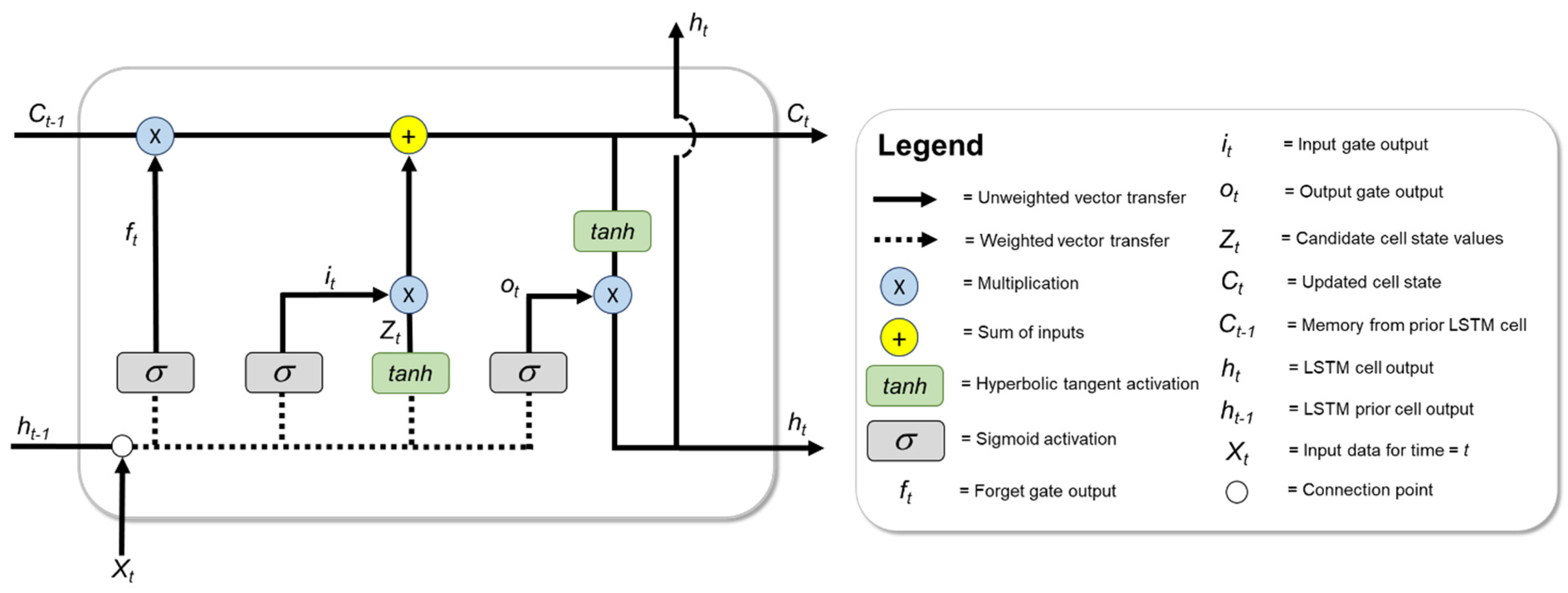
The LSTM concept was first introduced by Hochreiter and Schmidhuber in 1997 [129] and subsequently expanded and adapted by other since. LSTMs utilize a memory cell structure (Figure 5) to handle both shorter and long-term dependencies in time series datasets [130]. Short-term memory is captured as input from previous timestep cell output (ht−1). The long-term memory component is reflected in the cell state (Ct−1). LSTM memory cells have the ability to add or omit information to the cell state (i.e., Ct−1Ct), but only does so through carefully regulated structures called gates. Network gates consist of either sigmoid or hyperbolic tangent (tanh) activation coupled with pointwise multiplication operations.
Given the input data vector at time step t (Xt) and the previous time step LSTM cell output (ht−1) instituted, the hidden state output for current LSTM cell (ht) is calculated per the sequence discussed in the following bullets [129,134]:
  • First, the forget game (ft) is utilized to determine information that becomes omitted away from the cell state. New information introduced to the LSTM memory cell via ht−1 and Xt undergoes sigmoid transformation, the result of which is output between 0 (becomes fully omitted) and 1 (becomes fully included) for each number in the cell state Ct−1 per Equation (5).
    f t = σ ( U f X t + W f h t 1 + b f )
  • The second step involves determining new information to be stored in the cell state; this step occurs through two separate parts. The input gate (it) applies sigmoid activation to ht−1 and Xt and is used to inform values that will be updated in the cell state per Equation (6). Additionally, tanh activation generates a vector of new candidate values (Zt), which could be included in the cell state per Equation (7).
    i t = σ ( U i X t + W i h t 1 + b i )
    Z t = t a n h ( U z X t + W z h t 1 + b z )
  • The prior cell state Ct−1 is updated with new information to a new cell state Ct, via Equation (8):
    C t = f t C t 1 + i t Z t
  • The final step generates output (ht) that leverages memory from the cell. The output is a function of the new cell state Ct that undergoes some filtering via tanh activation as well as from output from the output gate (ot). The mathematical expressions for these steps are presented in Equations (9) and (10).
    o t = σ ( U o X t + W o h t 1 + b o )
    h t = o t × tan h   ( C t )
The equation variables pertaining to U and W include, respectively, the weights to the input data (Xt) and recurrent (ht−1) vectors. The b term is the bias for each gate.
Model architecture (Table 3) and hyperparameter settings were ultimately determined via trial and error opposed to a more systematic approach such as cross-validation (CV) with grid-search. The deep learning-based model requires a fairly extensive training duration (trained on a personal computer requiring approximately five seconds to train per epoch), therefore a holistic grid-search approach with CV to refine hyperparameter settings was not considered practical. Ultimately, the model network consists of four hidden units comprised of two stacked LSTM layers in a recurrent network fashion and two dense layers. All hidden layers utilize sigmoid activation. The stacked LSTM architecture was used given the noted successes demonstrated from comparable studies such as Sagheer and Kotb, Utgoff and Stracuzzi, and Jie et al. that found improved modeling generalization with deep, stacked structures over shallower architectures [31,32,135]. The hidden layer sizes were set to vary as a function of the input size (input shape = 24 features) by 2×, 4×, 4×, and 2× accordingly. A masking layer was used as the network input layer. The masking layer facilitates the omission of timesteps as part of sequence processing where input data are noted as missing. Prior to model training, well-level input data time series sequences are encoded via zero padding (post) into consistent sequence lengths [136]. Setting consistent sequence lengths for each well enables contiguous batch sizes as part of model training and resetting of LSTM cell states following each batch. The masking layer informs the network to skip timesteps where all input data = 0. The output layer enables regression-based prediction and is a dense layer with linear activation consisting of two neurons; one handling the predicted response for natural gas production and the other handling the predicted response for water production. All neurons are fully connected (no dropout applied) between model layers.
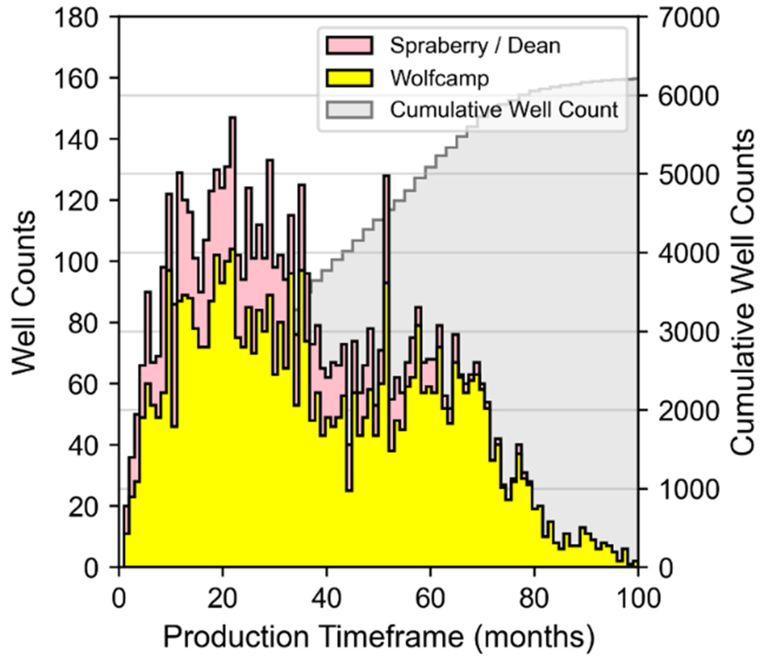
The inclusion of the dynamic well performance attributes of monthly oil, gas, and water production results in a dataset size with 561,661 observations (224,421 of which are not subject to zero padding) spanning 5561 wells at monthly resolution. Wells with less than 12 months of production data were omitted from model training. The portion of the project dataset used as part of the joint associated fluid production model development was randomly segmented into training, validation, and testing datasets through an 80/10/10 percentage-based split. This approach implements a training, validation, and testing split that maintains the temporal order of observations from the project dataset by keeping the entire productive timeframe for a given well intact. For instance, 10 percent of the dataset wells (based on American Petroleum Institute well ID number) were selected at random to isolate a test dataset. All associated static and dynamic data was appropriately cross-referenced to each well for use in model development. The same process was conducted on the remainder of the dataset to isolate an additional 10 percent to serve as a validation dataset. The data from the remaining 80 percent of the wells was used for training as part of model training.
Early stopping was applied as an additional regularization step to combat overfitting. This approach monitors the predictive performance of the model for every epoch during training against predictions on the held-out validation set (56,156 observations; 21,732 of which are not subject to zero padding) as a proxy for generalizing error. Model training was discontinued when validation error was minimized conditional to the use of a patience tolerance of 25 epochs. Model weight optimization was determined under mini-batch gradient descent using the “Adam” adaptive learning rate optimization algorithm [137], a batch size = 101 which is equal to the sequence length for each well with zero padding applied, and epochs = 1000. The learning rate was set at 0.0001. Keras default settings for first and second-momentum estimate decay rates as well as epsilon were used as part of Adam implementation. Once trained, model performance accuracy was evaluated on the 10 percent subset holdout test data (56,156 observations; 23,044 of which are not subject to zero masking). This step also provided additional confirmation that models were not over or underfit. The performance metrics used as part of model training, early stopping, and testing evaluation are discussed in Section 2.5.3.
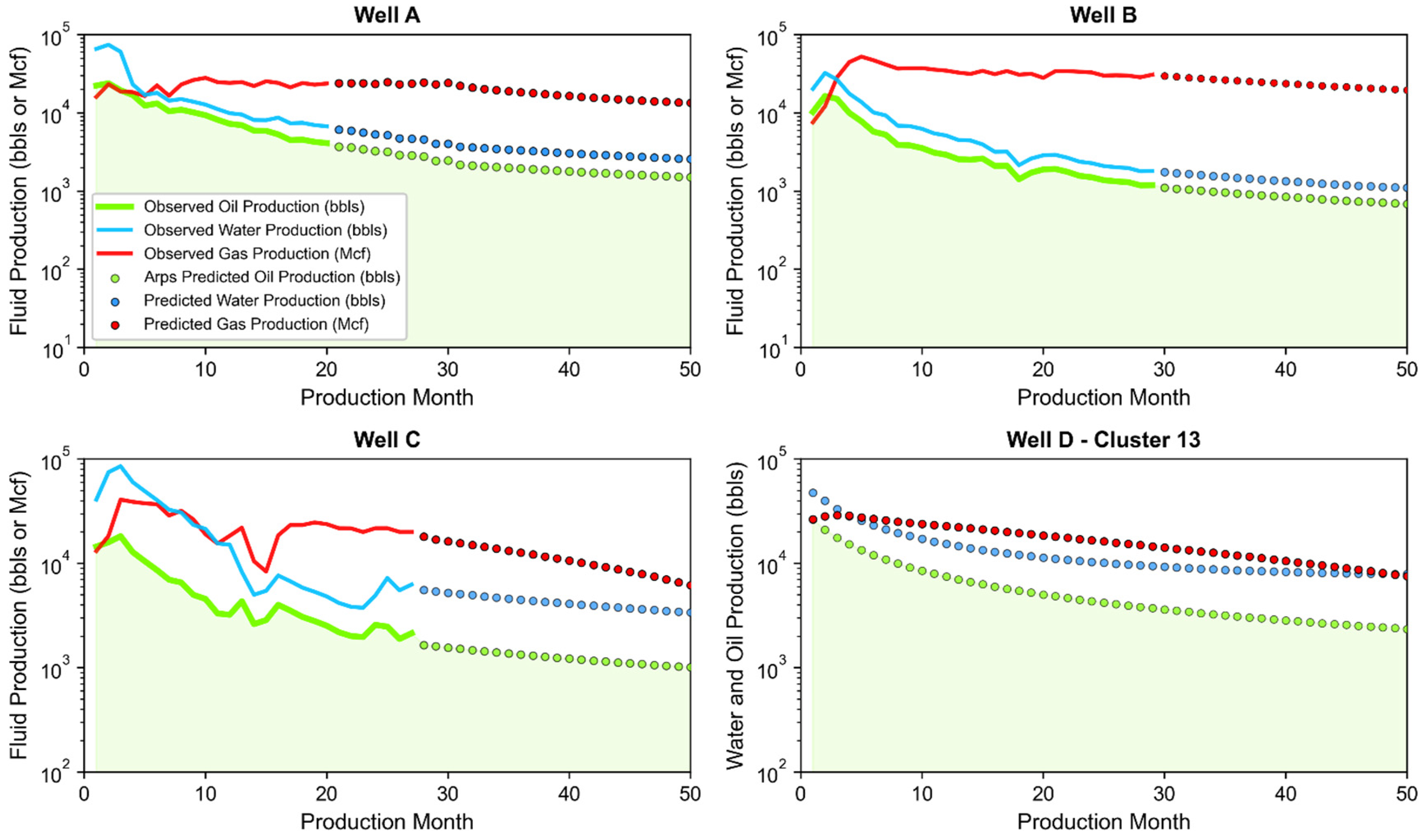
The model is easily employed to replicate a given well’s historic water and gas production with the use of required input data for the given month of interest. To generate prediction forecasts for future time instances, we employed a recursive prediction approach as explained by Ji et al. [138]. This strategy involves implementing the model in a t + 1 one step ahead prediction functionality under multiple iterations through the desired prediction horizon (t + h); where the prediction for the prior month (t) is used as an input for making a prediction for the following month (t + 1). Assuming well completion attributes do not change over time, these input features can be simply carried forward for all timesteps predicted. However, oil production is a dynamic, time-dependent input and required for forecasting water and gas volumes. Therefore, oil production forecasts that serve as inputs to the model must be derived from another means; potentially reservoir simulation output, a separate ML oil production predictive model, or even though analytical methods proposed by the likes of Fetkovich [88] and Arps [84].

2.5.3. Model Performance Evaluation

Our model performance was evaluated for the supervised learning-based joint associated fluid production model in two specific instances; (1) during model training against both the training and validation data sets and (2) through analysis of goodness-of-fit for simulated predictions against the test dataset. During model training, mean squared error (MSE) is used as the loss function. Performance of the model is quantified by MSE at each epoch against both the training and validation datasets; the latter provides an overall generalization error estimate as well as an indication to potential overfitting if training and validation MSEs begin to diverge substantially [139]. MSE is mathematically represented in Equation (11):
M S E = N 1 i = 1 N ( y i y ^ i ) 2
where N represents the length of the dataset, yi is the observed value, and y ^ i is the simulated or predicted response value.
The finalized joint associated fluid production model prediction performance was evaluated by making predictions against the test dataset. A combination of MSE, root mean squared error (RMSE), and R2 are used to evaluate model performance accuracy. RMSE corresponds to the mean error between predicted and observed values and reflects the variance of errors independent of sample size. As with MSE, smaller RMSE values are associated with reduced mean error between predicted and ground-truth data compared to model predictions where higher RMSE values occur [115]. RMSE provides a compliment to MSE and R2, one expressed in the units of the response variable(s) of interest. The R2 metric signifies the degree of correlation between simulated and observed values and is defined as the regression sum of squares (SSRegression) divided by the total sum of squares (SSTotal). R2 values are proportional to the data being evaluated and range between 0 and 1—higher values represent smaller variations between the ground truth data and predicted values and lower values may suggest little to no correlation exists. RMSE and R2 are described mathematically in Equation (12) and Equation (13) respectively:
R M S E = N 1 i = 1 N ( y i y ^ i ) 2
R 2 = S S R e g r e s s i o n S S T o t a l = 1 i = 0 N 1 ( y i y ^ i ) 2 i = 0 N 1 ( y i y ¯ ) 2
The overbar above variables per Equation (13) indicates the mean value for the complete dataset of ground truth observations considered.

2.6. Oil Forecasting

Monthly oil production estimates are needed in order to predict the associated gas and water production for wells in the study area using the LSTM-based deep learning time series joint associated fluid production model. We utilized the Arps decline curve model [84] to enable oil forecasts, either for (1) new (theoretical) wells where no historic production exists or (2) to extend historical production for existing wells. The Arps hyperbolic decline model, common for lower permeability shale production [140], is applied per Equation (14) to forecast oil production at the well level:
q = q i ( 1 + b D i t ) 1 b
where q is the monthly oil production (bbls/month), qi is the initial oil flow rate (bbls/month), b is the decline component which is dimensionless, Di is the initial decline constant (fraction/month), and t is the production month (month). The Arps models have shown to provide for reliable hydrocarbon history matches (even in cases with b > 1) and affords simplicity in their use [141]. However, the hyperbolic model can tend to over approximate reserves when extrapolated without constraints to long-term transient flow considerations [140,142]. Therefore, in this study, Equation (14) is only applied to forecast oil in short durations (limited to 60 months).

3. Results and Discussion

The following subsections outline key results as part of model development, evaluation, and application associated with the various machine learning workflows applied throughout the study to enable joint associated fluid production time series prediction capability.

3.1. Feature Selection Results

The feature selection step using RFECV and feature importance evaluation helps establish final sets of input features that can be applied as part of both the clustering evaluation and the development of the time series joint associated fluid production model. Results from this analytical step are described here, but can be found in detail in Appendix A. Informed from the findings from RFECV and importance evaluation, two distinct dataset aggregates (in addition to the set used for feature selection) are created; one for clustering and another for the time series-based joint associated fluid production model training and testing (Table 4).
Table 4 highlights the specific dataset features that make up each dataset aggregate. Based on findings from RFECV, 11 static features were selected and three omitted from the feature selection dataset for consideration in analysis moving forward. The down-selection includes omission of the features with the three lowest values of feature importance; which include percent in zone and the two categorical variables demarcating wells completed in either the “Spraberry/Dean” or “Wolfcamp” formations. The remaining data features are used for each of the following associated subsequent project tasks described in Section 3.2 (clustering) and Section 3.3 (the joint time series associated fluid production model).

3.2. Cluster Analysis

The results from the k-means clustering analysis are exhibited in Figure 6. Clustering results are presented in the context of both the Elbow method and Hartigan’s rule; both of which are used in tandem to select a representative number of well clusters from the study dataset where adding another cluster does not result in any substantial improvement to within-cluster sum of squared error. The visual heuristic results for the Elbow method suggest an appropriate cluster count falls somewhere between roughly 17 and 21 clusters (Figure 6A). The Hartigan Solution in Figure 6B explicitly identifies 18 clusters as optimal, and that adding the 19th cluster (where 19 is the k + 1 cluster where the Hartigan Index ratio between k and k + 1 is ≤10) results in negligible reductions to within-cluster sum of squared error.
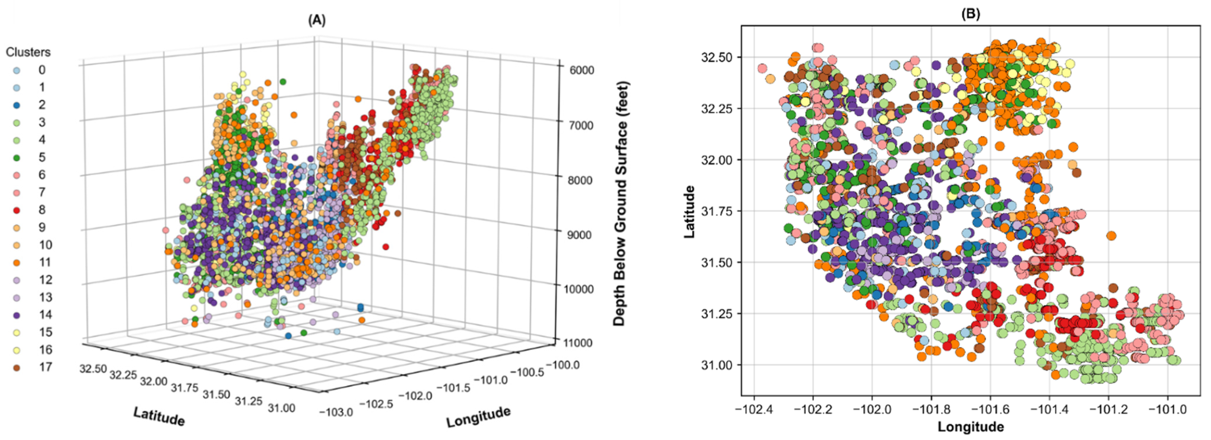
Wells within the study dataset were mapped to their corresponding cluster and then plotted to inspect clustering distribution across the study area (Figure 7). An initial observation is that the resulting distribution of well clusters appears influenced by more so than just three-dimensional placement characteristics. For instance, clusters five and 14 (dark green and dark purple respectively) span a large area and occur over a variety of burial depths. Although the specific reasoning for cluster assignment is not analyzed in detail as part of this study, it is likely that non-spatial features related to well completion design, well performance, and reservoir thickness were influential for the commonalities of wells in these clusters. However, in certain cases, wells within certain clusters are in close spatial proximity. This seems true for cluster eight (red) in the southern portion of the basin as well as cluster 15 (light yellow) in the northeast portion of the basin. Table A2, presented in Appendix C in this study, provides a summary of descriptive statistics for wells making up each cluster.
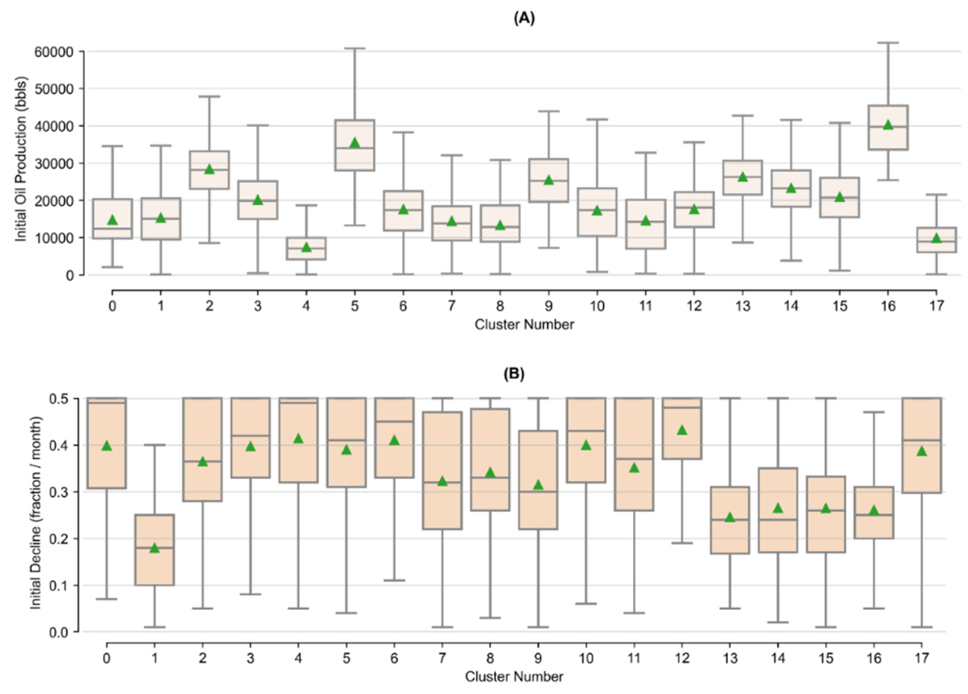
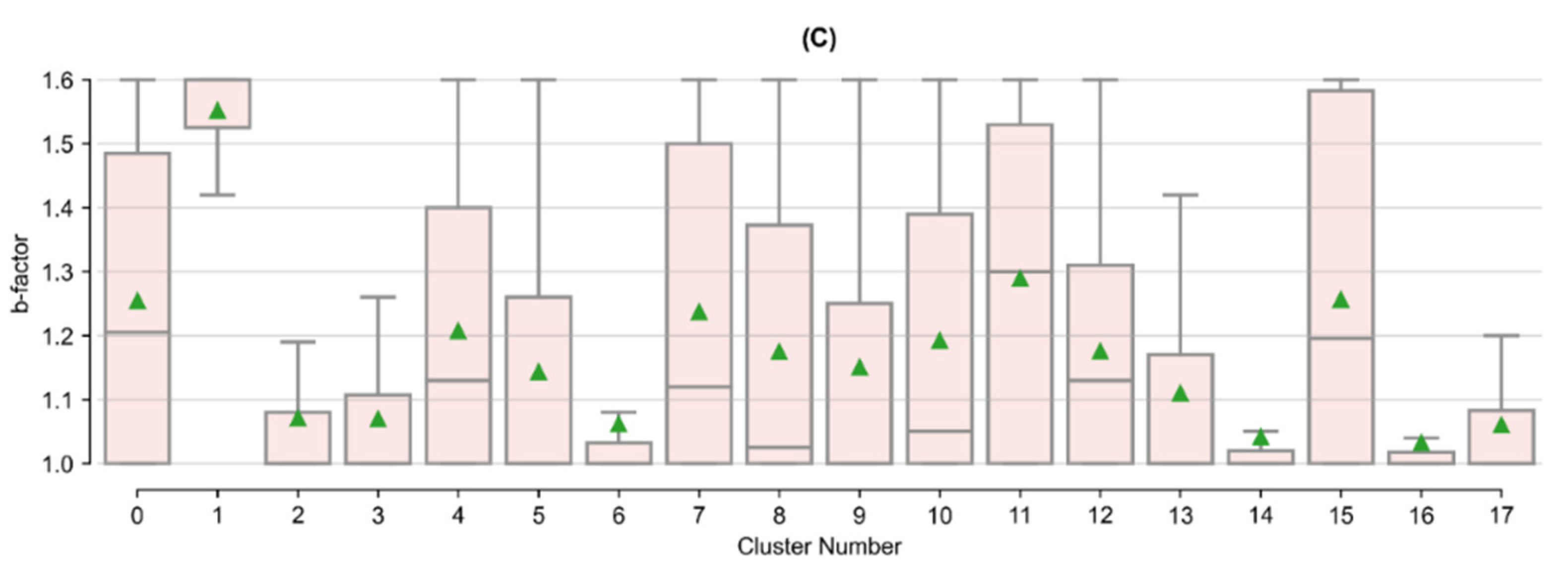
Arps decline properties can be extracted that are representative of the wells common to each cluster. These properties can then be used to forecast oil production at the well level using the Arps model per Equation (14). Figure 8 shows the distribution of the Arps decline properties for each cluster. Based on the distribution of these properties across clusters, oil production trends, and therefore associated gas and water, are expected to vary across clusters as well.
Multiple one-way Analysis of Variance (ANOVA) were conducted to evaluate the similarity or disparity of the Arps decline properties within and across each cluster as a way to statistically infer and differentiate variability in oil production trends across clusters. ANOVA is a parametric statistical technique used to compare different datasets—specifically equality associated with their means and the relative variance between them [143,144,145]. In this case, the independent variable evaluated was the cluster number, which included 18 levels [0 through 17]. The dependent variables included initial oil production, initial decline, and b-factor. Null hypotheses are rejected at a significance level of α = 0.05. ANOVA can provide insights into the overall significance of the well clusters and corresponding Arps decline properties, but the test cannot inform exactly where differences lie. Following ANOVA, Tukey’s Test [143,146] are used post-hoc to compare pairs of means for Arps decline attributes for which null hypotheses are rejected across each of 18 well clusters. The overall significance level is assumed α = 0.05 for testing pairwise mean comparisons. ANOVA results yielded significant variation for all Arps attributes among well cluster as a condition, p < 0.05. No Arps attribute was determined to be insignificant based on well cluster groupings. Therefore, a Tukey’s test was performed for each of the three Arps attributes across the 18 well clusters. The post hoc Tukey’s test (Table A1—shown in Appenix B) highlights which clusters, and therefore Arps decline attributes, differed significantly from cluster to cluster at α = 0.05. Clusters in Table A1 (shown in Appendix B) that do not share a Tukey’s Group are considered significantly different from each other. The Tukey’s Group lettering [A through L] are order based on the cluster with the highest mean value for the given attribute of interest relative to the other Tukey’s Groups. Tukey’s test results indicate that out of 18 different clusters, there are 12 statistically different cluster given initial oil production groupings (A–L), only eight statistically different cluster exist regarding initial decline (A–H), and 10 statistically different clusters in regard to b-factor (A–J). From an Arps model perspective, higher oil productivity is tied to larger values of initial oil production and b-factor and smaller values of initial decline. The analysis of variance and Tukey’s pairwise comparison tests are performed using Minitab 18 Statistical Software.

3.3. Joint Associated Fluid Production Model Training and Performance

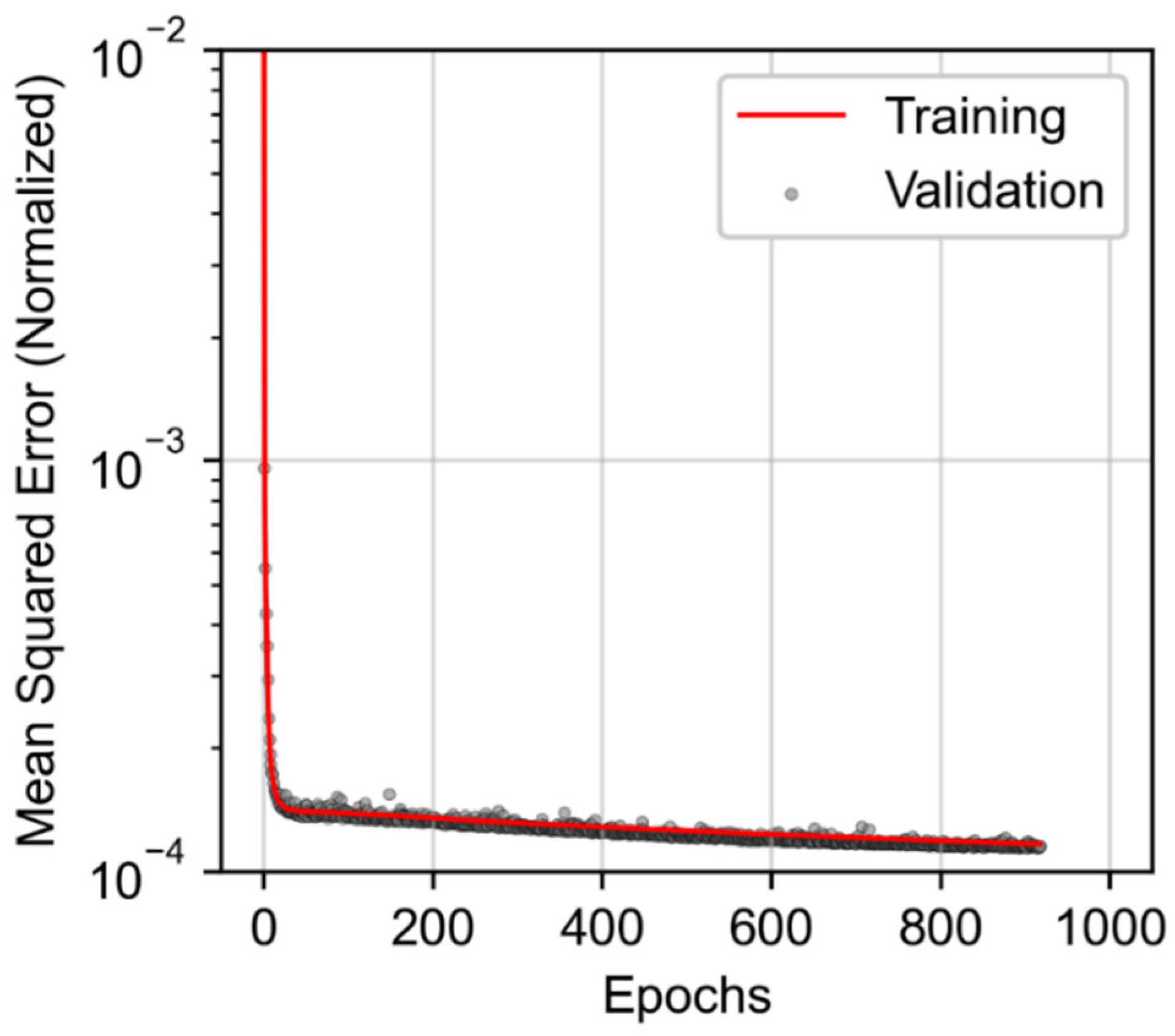
The predictive performance of the model as a function of training epoch is presented in Figure 9. The figure depicts the associated model loss (as MSE where model predictions, training data, and validation data values are in normalized form between 0 and 1) following the update of network weights prompted by new estimates of the error gradient following each training epoch. Given the consistency of the trends in validation and training loss, the model appears to demonstrate a suitable fit to the training data with no suggestion of over or underfitting, indicating the model’s overall effectiveness at generalizing associated fluid production. The application of early stopping ended model training after 918 epochs, resulting in a minimal generalization gap between training (1.16 × 10⁻⁴ MSE) and validation (1.15 × 10⁻⁴ MSE) performance.
The model’s predictive performance summary against both the training and test dataset set is compared in Table 5. Performance metrics presented in Table 5 are based on the response data transformed from normalized states per Equation (2) back into original units (Mcf and bbls) relative to each fluid stream. Overall, there is little disparity for model performance between the training and held-out test data, as well as marginal difference in the model’s ability to predict either water or gas.
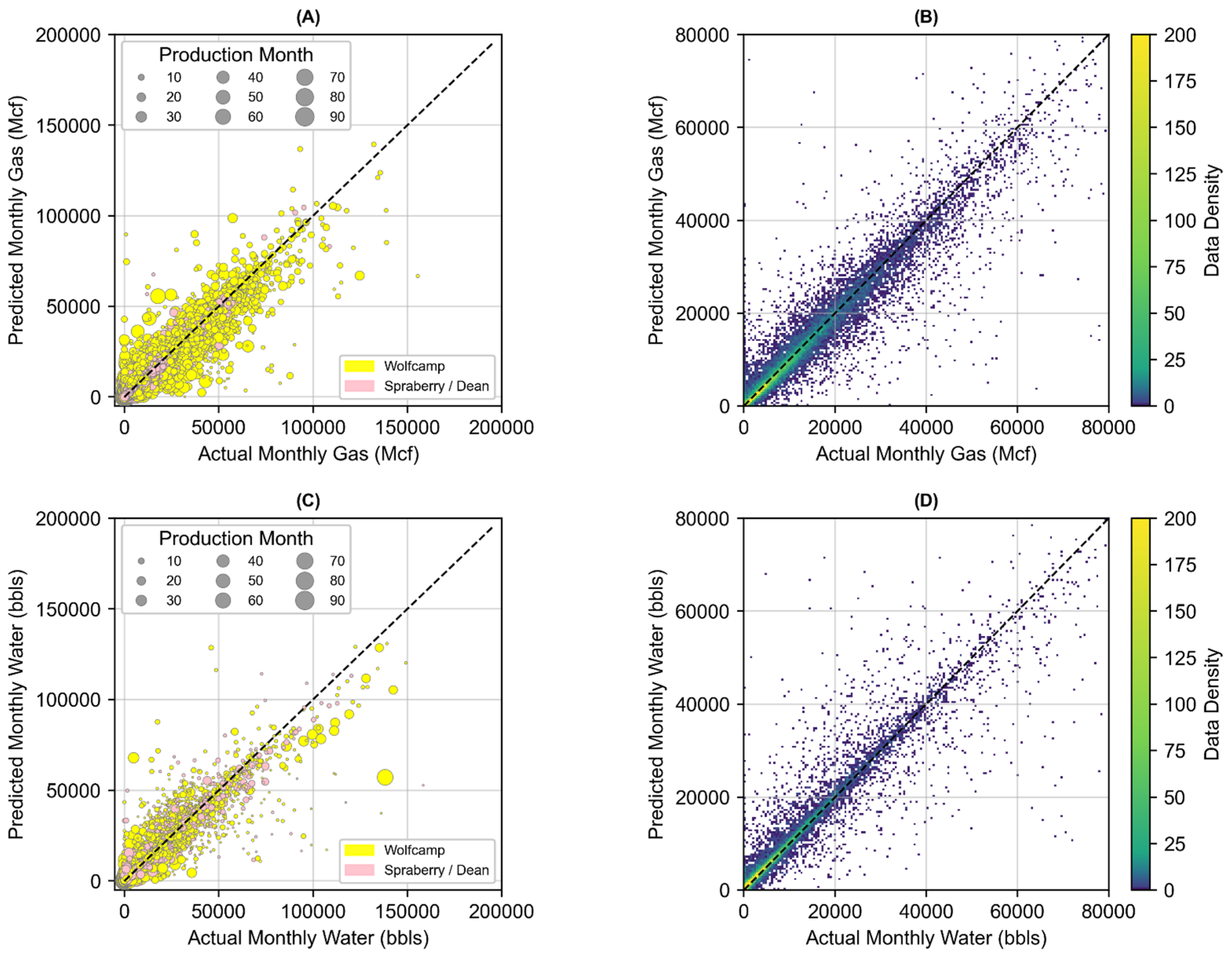
The prediction performance is visually compared with observed data from the test dataset in Figure 10. The parity plots (Figure 10A,C) provide a visual depiction of the model’s prediction to actual observed water or gas production on a monthly basis. The R2 metric (listed in Table 5) is used to quantify the correlation of actual to predicted monthly production data as part of the comparison in Figure 10. Model performance that would perfectly generalize production trends would have an R2 of one, and all data would fall exactly along the black dotted lines (i.e., 1-to-1 match) provided for reference. The model’s joint predictive capability is fairly strong overall; however, the model is slightly more accurate at predicting monthly gas on holdout data compared to water. Data is color coded by producing formation and sized by the production month to provide visual indicators for potential glaring trends in residual patterns. Fortunately, none seem to exist given that no irregularities in model residuals for either formation occur based upon visual inspection of the Figure 10 parity plots.
Figure 10B,D also features visual depictions of the density of data within each pixel of the x and y plotting area. Pixel coloration is based on the amount of data at a given x and y pixel. Viewed in isolation, the parity plots can be a bit challenging to assess the distribution of data around the 1-to-1 line given the large volume of data presented within and the spread throughout the plotting space. The density plots emphasize where higher aggregations of data fall and where model residual (variation from the 1-to-1 line) are most prominent. The majority of monthly gas and water predictions compared to test data actuals fall along the 1-to-1 line and residuals appear evenly distributed at all fluid production volumes. Density plots are zoomed in to focus on the 0 to 80,000 bbls or Mcf fluid volume range where the majority of test data occurs.
Figure 11 shows replication of the production history for water and gas for four different randomly selected wells within the test dataset. Predictions using the joint associated fluid production model stop when known production observations end. Solid lines in Figure 11 depict actual production data for oil (green), water (blue), and gas (red) from each of the four wells. Red and blue dots indicate prediction responses for LSTM-based joint associated fluid production model. For reference, a brief review of each well evaluated in Figure 11 is provided in the bullets below:
  • Well 1: Located in central Martin County producing from the Lower Spraberry with an 8409-foot perforated length, and placed at a total vertical depth of 9334 feet below ground surface.
  • Well 2: Located in northern central Midland County producing from the Wolfcamp B with a 7142-foot perforated length, and placed at a total vertical depth of 9673 feet below ground surface.
  • Well 3: Located in southeastern Midland County producing from the Wolfcamp B with a 6722-foot perforated length, and placed at a total vertical depth of 9383 feet below ground surface.
  • Well 4: Located in western Martin County producing from the Wolfcamp C with a 4855-foot perforated length, and placed at a total vertical depth of 10,031 feet below ground surface.
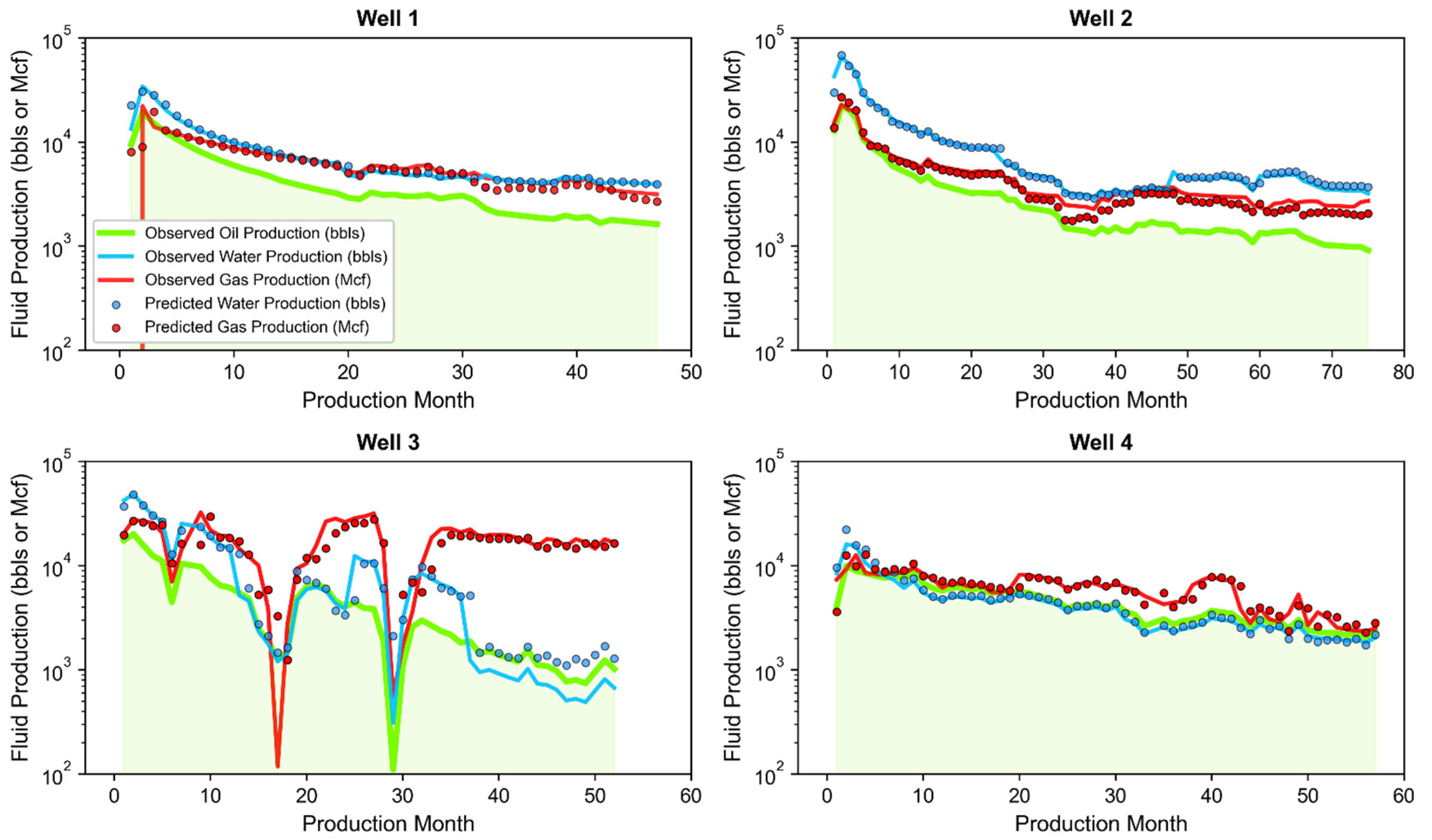
Figure 11. Replication of production history using the joint associated fluid production model for four test dataset wells.
Processes 10 00740 g011
Prediction results in Figure 11 are encouraging given the favorable replications of water and gas production profiles, even under circumstances that include irregular production trends. Worth noting is that the actual production trends for oil, water, and gas for each of the four wells evaluated are dissimilar in nature, yet the model is effective in replicating production profiles. Noted discrepancies in predictions to actual monthly flows seem to most commonly occur when highly transient (i.e., spikes or rapid falloffs) events transpire. However, given that the model input features are heavily dependent on prior timestep flows for oil, water, and gas, the model appears to adjust to transient events in making next timestep predictions.
Results to this point have been based on comparison of model prediction to replicate known production flows from wells within the test dataset. However, one of the functionalities of a time series-based model lies in the ability to forecast into the future where no observations exist. We implement the model under a recursive multi-step forecasting strategy as a way to predict gas and water production trends past existing wells’ known producing timeframes, as well as for generating production outlooks for new, theoretical well sites. Under this strategy, the model is used to make a prediction at time t, then the predicted values are appended to the input dataset to serve as prior month flow input data for predicting at time t + 1. Oil predictions via the Arps model are incorporated as part of the input dataset to enable prediction at time t, t + 1, through t + h where h = the total producing months prediction horizon. This process is repeated in a recursive manner until the t + h is reached. A simple exponential forecast smoothing function [147] is applied at t > 24 months where the t + 1 prediction is a sum of model’s t + 1 estimate plus the prior t value in a weighted 90/10 percentage contribution. Past the t > 24 months producing timeframe, observed monthly water and gas values for wells in the study dataset are frequently at the scale (or lower) of the model prediction error (roughly 2500 to 2600 RMSE in Mcf or bbls per month as per Table 5). The smoothing approach ensures stability in the forward predictions as part of the recursive implementation of forecasts.
Since the joint associated fluid production model is a purely data driven model, it may be limited at making sound predictions for: (1) circumstances where low quantities of data to train models exists; and (2) timeframes that extend far beyond the extent of the production durations for wells in the training data. Over 80 percent of the wells in the study dataset have well production timeframes less than 60 months (Figure 12). After 60 months, the volume of well data becomes sparse, especially for Spraberry/Dean wells. Additionally, as discussed in Section 2.6, the application of the Arps model over the long-term with high b-factors using the hyperbolic model may overestimate hydrocarbon production. Plus, the recursive prediction strategy can suffer from error accumulation and propagation, particularly when the forecasting horizons increase [148,149]. These potential limitations serve as the basis for setting our constraint to limit forecasts to shorter-term predictions.
Results in Figure 13 show forecasted production for oil, water, and gas for four different wells; three of which (Wells A, B, and C) are existing wells selected from the test dataset and the fourth (Well D) is a theoretical well based on the dataset mean values for input features common to Cluster 13 (see Table A2 in Appendix C). Cluster 13 was selected as an example for analysis here since it contains a realitvely large mean initial oil production and encompases a substantial portion of the well count from the study dataset; the majority of which are Wolfcamp wells. Forecasts using the joint associated fluid production model intentionally stop at 50 months under all cases regardless of well production history. Solid lines in Figure 13 depict actual production data for oil (green), water (blue), and gas (red). Red, green, and blue dots represent the montly forecasts for the Arps (oil) and joint associated fluid production model (water and gas).
For reference, a brief review of each well evaluated in Figure 13 is provided in the bullets below:
  • Well A: Located in northern Upton County producing from the Wolfcamp A with a 7745-foot perforated length, and placed at a total vertical depth of 9476 feet below ground surface.
  • Well B: Located in western Irion County producing from the Wolfcamp B with a 10,114-foot perforated length, and placed at a total vertical depth of 6709 feet below ground surface.
  • Well C: Located in southern Glasscock County producing from the Wolfcamp A with a 10,261-foot perforated length, and placed at a total vertical depth of 7976 feet below ground surface.
  • Well D: Theoretical well representative of Cluster 13 (see Table A2 in Appendix C for specifics) based on a 9870-foot perforated length, an initial monthly oil production of 26,324 bbls, and placed at a total vertical depth of 9128 feet below ground surface.

4. Oil, Gas, and Water Production Outlook

The joint associated fluid production model has been applied in combination with the Arps model to generate oil, gas, and water production outlooks for each of the 18 clusters identified in Section 3.2 (Table 6). The outlooks were generated at the well level for a single hypothetical well representing each cluster. The hypothetical wells that represent each cluster are attributed well completion, decline curve, and spatial and reservoir attributes set to the cluster’s mean value for each. Outlooks include the cumulative first and five-year estimates for production totals (Table 7). The suite of data presented in Table A2 in the Appendix C is a digest of attribute statistics (most notably mean, standard deviation, and interquartile range [IQR]) as well as cumulative production outlook estimates from the combination of the Arps and joint associated fluid production models for each cluster. Additionally, this collection of data is intended to serve as a guiding resource for assessing the potential volumes of produced fluids associated with oil production in the Midland Basin based on well completion design considerations and placement within the basin.
The predictions for each cluster appear aligned to typical volumes of in-field production trends for wells in the Midland Basin. For instance, our predicted production totals in Table 7 when compared in the context of water-to-oil and gas-to-oil ratios appear in range with those reported in literature [49,150,151,152]. For instance, the ratios from estimated production throughout the first producing year from Table 7 values range from approximately 1.57 to 2.68 bbls/bbls for water-to-oil across clusters (with a mean of 2.03]) and 1.43 to 3.15 thousand cubic feet (Mcf)/bbl for gas-to-oil across clusters (with a mean of 1.94). Cumulative produced water and gas (to-oil) estimates after 5-years or production are in the ranges reported by Rassenfross [49] and Kondash et al. [79] respectively. Additionally, the predictions capture increasing gas-to-oil ratio trends as wells becomes older [153]; not uncommon to unconventional plays, particularly when production causes reservoir pressures to fall below the bubble-point [154].
Table 7 highlights several major takeaways from the digest presented in Table 7; particularly the cluster groups estimated to have the highest or lowest totals for (1) oil, gas, and water production per well, as well as (2) associated fluids normalized to a barrel of oil produced. The results indicate that Cluster 16 is the best oil producer for the first producing year and through five years of production. Cluster 16 also is noted to be comparatively efficient versus other clusters based on the ratio of associated fluids volumes produced with oil; particularly for the first year of production. Cluster 4 is the lowest oil producing cluster and highly inefficient regarding the associated fluids volumes produced with oil. Cluster 1 produces some of the largest volumes of associated water and gas, but only produces oil near the average for all clusters. As a result, Cluster 1 is one of the most inefficient clusters in terms of oil to gas and oil to water production ratios in addition to Cluster 4. Clusters 3, 5, 11, and 16 are noted as relatively more “efficient” clusters than others based on their higher oil to gas and oil to water producing ratios for both the first producing year and through 5 years. Overall, clusters 1, 4, 6, 8, and 17 appear to be the least efficient regarding associated fluid production normalized to oil.
We performed one last analytical case study using the data in Table 7 to generate production volume outlooks in regards to associated fluid production in the Midland Basin. Specifically, first and five-year production outlooks are generated at the basin-level under three development scenarios that comprise of a new fleet of wells built on different contributions of wells common to certain cluster groups. The scenarios include:
  • Scenario 1: high efficiency development—25 percent contribution of wells from clusters 3, 5, 11, and 16
  • Scenario 2: low efficiency development—20 percent contribution of wells from clusters 1, 4, 6, 8, and 17
  • Scenario 3: diversified development—contribution of wells from each cluster randomly assigned under equal probability per cluster
An average of 1842 wells have been spud per year in Spraberry/Dean and Wolfcamp formations in the Midland Basin from 2017 to 2019 based on the study dataset. The generated outlooks under each of the three scenarios evaluated are therefore based on a theoretical new well fleet of 1842 wells in each scenario. Production outlooks for oil, water, and gas volumes produced from the new well fleet in the first year and through five years of production are shown in Figure 14.
First year production volumes range from approximately 132,000 to 275,000 Mbbls oil, 304,000 to 473,000 Mbbls water, and 335 to 405 Bcf of gas across the three scenarios constructed. Production volumes through five years extend from 276,000 to 535,000 Mbbls oil, 599,000 to 1,000,000 Mbbls of water, and 847 to 969 Bcf of gas. Results emphasize the notion that development choices regarding well design and placement (varied here by clusters implemented) have considerable implications on resulting fluid production outlooks. Worth noting is that under Scenario 1, where well deployment is limited to the clusters with the highest oil to associated fluid efficiencies, the largest volumes of associated water are produced compared to other scenarios. Associated gas, however, is the lowest out of all three scenarios. On the other hand, well development under Scenario 2 results in the lowest comparative volume of oil produced, but also generates the highest 5-year volumes of associated gas compared to other scenarios. Additionally, produced fluid volumes are likely to scale accordingly based on the number of wells that come online. Additional deployment scenario analyses could be explored using data in Table A2 to evaluate the influence of coupled well design, placement, and volume on produced fluid outlooks. Based on the approximate percentage of gas flared to gas produced in the Midland Basin per Leyden (2.35 percent of total), roughly 20 to 23 Bcf of gas would be flared over the five-years of production based on the results presented in Figure 14.
While this is a relatively straightforward example, it is nonetheless effective for quantifying produced volumes of both natural gas and water based on potential O&G development considerations. The outlooks can aid operators when formulating management or remedial solutions for the volumes of fluids expected. However, this analysis only includes production outlooks for the new wells considered and does not incorporate legacy production from wells producing prior to the installation of the new well fleet or those wells that come online afterwards. Production outlooks for natural gas or oil are highly dependent on a multitude of factors, including the typical production profiles of individual wells over time, the cost of drilling and operating those wells, the prospective economic return generated by those wells, the prevailing economic conditions related to O&G supply and demand, the intensity in which new wells are drilled, completed, and turned online, and the available prospective area remaining for a given play [29,155,156,157]. Forecasting associated water and gas would also be subject to similar factors. Therefore, alternative scenario formulations could be used to reflect different basin development outlooks than the one’s analyzed here.

5. Conclusions

In this paper, we have introduced a data-driven modeling framework that combines supervised and unsupervised ML approaches. The findings from this study suggest that the approach and combination of machine learning strategies provides for a capable time series predictive model that can be used to either reproduce or forecast cumulative volumes of natural gas and water produced alongside oil at the well level. The intent of the supervised learning component was to produce a deep learning-based model with the capability to generate reliable estimates of produced water and natural gas in a time series manner based on well completion and placement decisions. The unsupervised learning aspect established groupings of related wells, enabling a straightforward method to deduce Arps Decline, well completion, and reservoir and spatial attributes characteristic of each cluster group. The ensemble of the supervised and unsupervised elements of this work facilitates a means to forecast oil, water, and natural gas production at the well level as influenced by specific development considerations. Well level three-stream production volumes can be used to scale up outlooks at the pad, field, or basin-level (as demonstrated in Section 4). The framework has been applied to the producing extent of the “Wolfberry” within the Midland Basin. However, since the overall analytical approach is based on readily available datasets common to public sources, it could be easily modified for use in other mature unconventional O&G producing regions.
Major environmental concerns regarding shale O&G development are associated to water usage, induced seismicity via wastewater disposal, and flaring (and possible venting) of produced natural gas. The framework presented in this study can be leveraged to help support the formulation of management and/or remedial strategies based on the volumes of fluids expected from unconventional O&G development operational conditions. Study results have highlighted the variability in noted water and gas volumes produced depending on wellbore design and placement considerations—a finding which suggests that forecasting is a nontrivial task. Table 6, Table 7, and Table A2 provide quantitative insight that can reduce the burden in estimating associated fluid production for future wells. Data compiled in Table A2 summarizes the potential volumes of produced fluids associated with oil production across the study area given well completion design considerations and placement within the basin. These data can be used to build out three-stream fluid production outlooks for the Midland Basin. Forward-looking production outlooks for oil, water, and natural gas as highlighted in Figure 14 are highly dependent on the nature of well design and placement considerations of the subsequent fleet of wells (as well as legacy production from existing wells). However, many of these design choices that would determine the composition of the out-year fleet of wells can be strongly influenced by external economic or market-driven factors.
Potential follow-on work could be beneficial in addressing possible limitations and imposed constraints in the research presented here; as well as build off of the opportunities this study creates. For instance, the within-cluster variation in decline curve, well completion, and spatial and reservoir attribute data noted in Table A2 affords the opportunity towards a more stochastic analytic approach as a complement to the deterministic strategy using mean values presented in this study. A potential area for improvement to the study in regards to the model development pertains to limited access to geologic data which could be used as inputs. Readily available geologic data at the well level in large volumes is uncommon. Nevertheless, the inclusion of additional geologic characteristics that are known controlling factors to unconventional oil and gas recovery [158] may provide added utility in data-driven ML modeling. Additionally, our study was without access to key time series data pertaining to how wells were operated (i.e., choke, bottom-hole pressure, lift type), the result of which presents a challenge in integrating the human element as part of the forecasting component. In regards to forecasting oil production, gradual or abrupt changes in the producing rate of a well due to reservoir depletion, fluctuation in bottom-hole producing pressure, and changes in conditions in or immediately adjacent to the wellbore are not directly considered when using the Arps models alone. Lastly, potential model performance improvement gains might be realized thorough the development of separate models for predicting monthly water and gas individually instead of in joint fashion.

Author Contributions

Conceptualization, D.V.; methodology, D.V. and V.K.; validation, D.V. and V.K.; formal analysis, D.V.; investigation, D.V. and V.K.; resources, D.V. and V.K.; data curation, D.V.; writing—original draft preparation, D.V.; writing—review and editing, V.K.; visualization, D.V.; supervision, V.K. All authors have read and agreed to the published version of the manuscript.

Funding

This research received no external funding.

Institutional Review Board Statement

Not applicable.

Informed Consent Statement

Not applicable.

Data Availability Statement

The study well data utilized for this study was obtained from the O&G data vendor DrillingInfo/Enverus through a subscription service. Therefore, the study dataset cannot be made publicly available.

Acknowledgments

The authors would like to thank Enverus and DrillingInfo for their generosity in providing access to the data used as part of this study. Additionally, the authors would like to thank William Harbert of the University of Pittsburgh’s Department of Geology and Environmental Science and Carla Ng of the University of Pittsburgh’s Civil & Environmental Engineering Department for the constructive reviews which greatly improved the quality of manuscript.

Conflicts of Interest

The authors declare no conflict of interest associated with this research.

Unit Conversions

The units used in this manuscript are commonly used industry standards for the oil and gas sector in the United States. Conversion factors to the international system of units are as follows: 1 barrel = 0.159 cubic meters; 1 foot = 0.3048 m; 1 cubic foot = 0.0283 cubic meters; 1 square mile = 2.589 square kilometers.

Appendix A. Feature Selection Results Overview
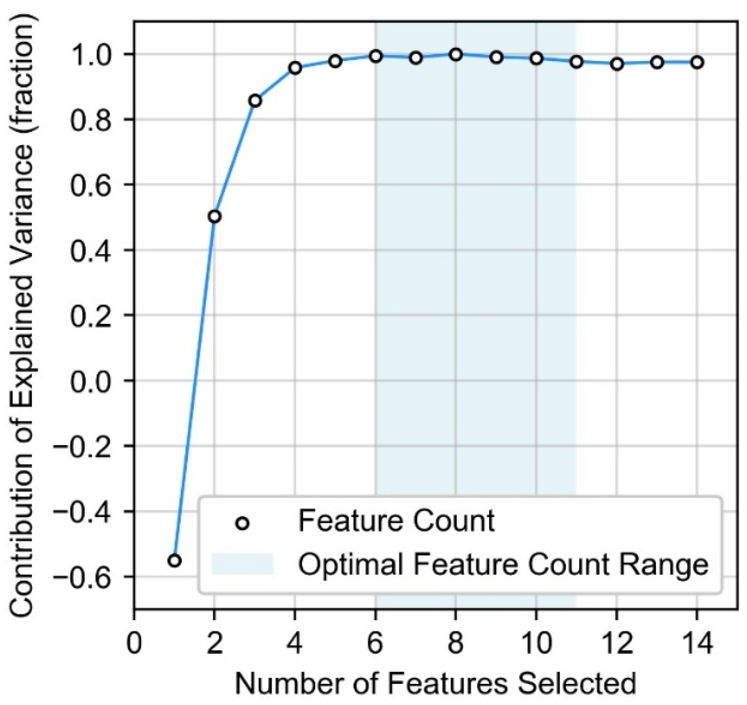
The hyperparameter combination selected via grid search cross-validation for the RF estimator used as part of RFECV included a formulation of 5050 trees and a minimum of two samples to split an internal node.
Figure A1 depicts the predictive performance of the RF estimator based on the number of features employed as part of training and cross-validation testing. For this study, explained variance for each model iteration across the range of features selected are normalized relative to the number of features included resulting in the highest explained variance. As a result, the number of features resulting in the estimator with the highest explained variance has value equal to 1, and all others less than 1. Once the number of features is reduced below six, the estimator’s predictive performance begins to diminish as more features are omitted as part of estimator training. In contrast, estimator performance gains are marginal at best when the number of features included in training are greater than six; with an optimal range between six and eleven features.
Figure A1. Effect of feature inclusion relative to the highest feature count score.
Processes 10 00740 g0a1
The ranking importance of each feature based on the estimator formulation with all 14 features included as part of training is presented in Figure A2. The ranking is based on the “relative” importance of each feature to that of the feature with the highest importance. The values for importance for each feature are normalized relative to the most import feature then scaled by 100. As a result, the feature with the highest importance has a value equal to 100, and all others less than 100. Examination of the feature importance ranking and magnitude indicates that oil production (reflected as Top 12 Months Oil) is the most important estimator feature for joint prediction of Top 12 Months Water and Top 12 Months Gas (static proxies for Monthly Gas and Monthly Water dynamic data features). The Top 12 Months Oil static data feature serves as a proxy for Monthly Oil, which is a dynamic feature that changes with time. The following three features (latitude, longitude, and true vertical depth) specify the three-dimensional coordinates for well horizontal placement within the basin. This finding suggests that the associated geological characteristics of the producing reservoirs which vary spatially and with burial depth are important contributors to the associated fluid response. Feature ranks five through seven (perforation length, water per foot, and proppant per foot) are notable well completion design attributes.
Figure A2. Summary of feature importance for the RF estimator used as part of RFECV.
Processes 10 00740 g0a2
The feature importance values in Figure A2 are used in concert with RFECV results from Figure A1 to inform the feature selection process. As a result, 11 static features are selected and three omitted from feature selection dataset for consideration in the clustering and time series analysis. This down-selection includes omission of the features with the three lowest values of importance; which include percent in zone and the two categorical variables demarcating wells completed in either the “Spraberry/Dean” or “Wolfcamp” formations. The removal of three features and inclusion of the remaining 11 coincide with the RFECV upper bound feature range count presented in Figure A1 where explained variance remains high.
As mentioned in Section 3.1, the feature selection step helps to systematically finalize sets of input features that can be applied as part of both the clustering evaluation (Section 3.2) and the development of the time series joint associated fluid production model (Section 3.3).

Appendix B. Tukey’s Test Results on Arps Attributes by Cluster

The results from the Tukey’s test performed one each of the three Arps attributes across the 18 well clusters is presented in Table A1. The post hoc Tukey’s test highlights which clusters, and therefore Arps decline attributes, differed significantly from cluster to cluster at α = 0.05.
Table A1. Descriptive statistics and results from Tukey’s test on decline curve attributes across well clusters.
Cluster NumberInitial Oil Production (bbls)Initial Decline
(Fraction/Month)
b-Factor
CountMeanStdev.Tukey’s GroupMeanStdev.Tukey’s
Group
MeanStdev.Tukey’s
Group
08414,8167459H, I, J, K0.400.12A, B, C, D1.250.24B, C, D, E
125915,3647653J, K0.180.09H1.550.08A
224628,3827826C0.360.12D, E1.070.14I, J
359420,1487935G0.400.11B1.070.13I, J
446074814835M0.410.12A, B1.210.22C, D, E, F
557435,57710,694B0.390.11B, C, D1.140.20G, H
632817,6257588H, I0.410.10A, B1.060.13I, J
760914,4427392K0.320.14F1.240.25B, C
823013,4087594K0.340.12E, F1.170.22D, E, F, G
917325,5068124D, E0.320.13F1.150.23F, G, H
1051517,3538606H, I, J0.400.11B1.190.23E, F
1110114,6308813I, J, K0.350.13C, D, E, F1.290.24B
1248517,6666449H0.430.08A1.180.18F, G
1330426,3246777C, D0.250.11G1.110.18H, I
1455423,3467579E, F0.270.13G1.040.09J
1516020,9718156F, G0.260.12G1.260.25B, C
1634640,3428293A0.260.10G1.030.08J
1718899595386L0.390.11B, C, D1.060.11I, J

Appendix C. Well Cluster Statics and Production Outlooks

Table A2. Inventory of descriptive statics, 1st year, and cumulative 5-year production estimates for a hypothetical representative well within each Midland Basin Well Cluster.
Data GroupDataset FeatureStatisticMidland Basin Well Cluster Number: 0 through 8
012345678
Well Completion AttributesPerforation Length (foot)Mean6782879195937928771910,061917771399663
Stdev.199017701319166515631502185615651763
IQR29852704113223781065756258115451756
Proppant per foot (lbs)Mean181816981764165913031845193814772283
Stdev.570391331349413389428395394
IQR487468319430495367459517546
Water per foot (bbls)Mean46.845.650.740.628.247.849.637.251.4
Stdev.15.310.39.012.28.310.110.910.69.3
IQR9.812.411.615.59.113.013.113.28.7
Additive per foot (bbls)Mean12.12.82.94.11.82.63.53.22.1
Stdev.3.91.81.53.11.31.63.31.81.2
IQR3.92.52.04.92.12.32.52.61.3
Azimuth (degrees)Mean165.1162.4162.6162.6180.3162.6178.9162.6180.8
Stdev.7.03.73.73.63.43.35.93.33.1
IQR3.24.23.44.14.34.05.12.34.1
Nearest Well Distance (feet)Mean844288254261550259523382388
Stdev.1013384307324473269441556428
IQR1185307277267519295413390453
Decline Curve AttributesInitial Oil Production (bbls)Mean14,81615,36428,38220,148748135,57717,62514,44213,408
Stdev.7459765378267935483510,694758873927594
IQR10,63511,15510,17310,197589513,45510,74892339916
Initial Decline (fraction/month)Mean0.400.180.360.400.410.390.410.320.34
Stdev.0.120.090.120.110.120.110.100.140.12
IQR0.200.150.220.170.180.190.170.260.22
b-factorMean1.251.551.071.071.211.141.061.241.17
Stdev.0.240.080.140.130.220.200.130.250.22
IQR0.500.080.080.110.400.260.040.500.39
Spatial and Reservoir AttributesTrue Vertical Depth (feet)Mean892489648947931071128811715090207460
Stdev.752630626470741785620771577
IQR798848884563963129610181174686
Thickness (feet)Mean443398471320774375633374553
Stdev.15713711596146108207134191
IQR20914813714859136338185361
Surface Hole Latitude (degrees)Mean31.6431.9231.7032.0831.1532.0831.3831.9831.32
Stdev.0.320.280.170.260.120.280.230.290.14
IQR0.440.450.190.470.190.470.380.560.19
Surface Hole Longitude (degrees)Mean−101.93−101.93−101.81−102.08−101.33−101.87−101.26−101.90−101.58
Stdev.0.280.190.220.140.230.240.180.290.16
IQR0.320.290.320.210.260.420.300.530.15
WolfcampCount68168223315456419326445230
S.berry/DeanCount169123280415521640
Production Forecast per WellCumulative Oil (Mbbls)1st year7711114710038181868273
5-years15428227518374346156169145
Cumulative Gas (Bcf)1st year0.160.200.250.150.120.270.250.130.22
5-years0.290.580.620.230.230.600.760.210.79
Cumulative Water (Mbbls)1st year154230268181102304200162182
5-years289587545347175659358324328
Data GroupDataset FeatureStatisticMidland Basin Well Cluster Number: 9 through 17
91011121314151617
Well Completion AttributesPerforation Length (foot)Mean830776777253722598708762944899727417
Stdev.181419702103179411551469189213331605
IQR2711293342122361563231326127401549
Proppant per foot (lbs)Mean328117281609144117521812178718281342
Stdev.775464535547336359412490394
IQR872677759687305413507407532
Water per foot (bbls)Mean71.439.440.636.649.448.844.948.032.8
Stdev.19.711.214.914.08.010.712.510.28.6
IQR23.213.817.318.98.79.615.510.67.8
Additive per foot (bbls)Mean4.92.14.22.12.22.32.12.91.9
Stdev.2.91.53.41.31.41.51.51.71.2
IQR3.01.83.81.62.02.32.01.92.0
Azimuth (degrees)Mean163.2162.6168.0162.2162.9162.4163.3162.8180.8
Stdev.5.52.98.83.33.73.43.33.62.1
IQR4.62.517.63.63.53.83.24.42.2
Nearest Well Distance (feet)Mean3953925658303328243486278343
Stdev.5424731942354308306764270438
IQR4194042770285386259511316438
Decline Curve AttributesInitial Oil Production (bbls)Mean25,50617,35314,63017,66626,32423,34620,97140,3429959
Stdev.812486068813644967777579815682935386
IQR11,76212,79913,55593249246978510,74411,7956533
Initial Decline (fraction/month)Mean0.320.400.350.430.250.270.260.260.39
Stdev.0.130.110.130.080.110.130.120.100.11
IQR0.210.180.250.130.150.180.170.110.21
b-factorMean1.151.191.291.181.111.041.261.031.06
Stdev.0.230.230.240.180.180.090.250.080.11
IQR0.260.390.540.310.170.020.590.020.09
Spatial and Reservoir AttributesTrue Vertical Depth (feet)Mean907878838340923891289123775189637523
Stdev.6095681101465424511727587723
IQR7845271950555540673956962961
Thickness (feet)Mean503384463541653380369356477
Stdev.20910318314517610311186151
IQR244132224168289119110115254
Surface Hole Latitude (degrees)Mean31.8332.2331.8031.6831.6031.9132.3332.0931.39
Stdev.0.330.300.480.160.160.270.240.240.18
IQR0.560.470.870.240.260.430.210.390.27
Surface Hole Longitude (degrees)Mean−101.90−101.58−101.70−101.89−101.82−102.01−101.62−101.94−101.38
Stdev.0.200.140.320.150.120.160.220.190.17
IQR0.250.120.560.180.150.190.270.370.17
WolfcampCount1373568945930132188227188
S.berry/DeanCount3615912263223721190
Production Forecast per WellCumulative Oil (Mbbls)1st year14189808716013512923750
5-years28117316816732826527946591
Cumulative Gas (Bcf)1st year0.260.140.120.150.310.220.220.340.12
5-years0.570.190.160.270.910.500.450.850.27
Cumulative Water (Mbbls)1st year271185170171306249265373111
5-years574364287332684515621879178

References

  1. U.S. Department of Energy. Ethane Storage and Distribution Hub in the United States; U.S. DOE: Washington, DC, USA, 2018.
  2. Pirog, R.; Ratner, M. Natural Gas in the U.S. Economy: Opportunities for Growth; Congressional Research Service: Washington, DC, USA, 2012.
  3. U.S. Energy Information Administration. Today in Energy: Both Natural Gas Supply and Demand Have Increased from Year-Ago Levels. U.S. Department of Energy. 4 October 2018. Available online: https://www.eia.gov/todayinenergy/detail.php?id=37193 (accessed on 31 March 2019).
  4. Clemente, J.U.S. Natural Gas Demand for Electricity Can Only Grow. Forbes. 15 January 2019. Available online: https://www.forbes.com/sites/judeclemente/2019/01/15/u-s-natural-gas-demand-for-electricity-can-only-grow/#27b0ba844c74 (accessed on 31 March 2019).
  5. Aadnøy, B.; Looyeh, R. Petroleum Rock Mechanics, 2nd ed.; Gulf Professional Publishing: Oxford, UK, 2019. [Google Scholar]
  6. United States Geological Survey, U.S. Department of the Interior. What Is Hydraulic Fracturing? Available online: https://www.usgs.gov/faqs/what-hydraulic-fracturing?qt-news_science_products=0#qt-news_science_products (accessed on 21 November 2020).
  7. Hyman, J.; Jiménez-Martínez, J.; Viswanathan, H.; Carey, J.P.M.; Rougier, E.; Karra, S.; Kang, Q.; Frash, L.; Chen, L.; Lei, Z.; et al. Understanding hydraulic fracturing: Amulti-scale problem. Philos. Trans. Ser. A Math. Phys. Eng. Sci. 2016, 374, 20150426. [Google Scholar] [CrossRef] [PubMed]
  8. Aminzadeh, F. Hydraulic Fracturing, An Overview. J. Sustain. Energy Eng. 2019, 6, 204–228. [Google Scholar] [CrossRef]
  9. U.S. Environmental Protection Agency. The Process of Unconventional Natural Gas Production. 22 January 2020. Available online: https://www.epa.gov/uog/process-unconventional-natural-gas-production (accessed on 21 November 2020).
  10. Perrin, J. Horizontally Drilled Wells Dominate U.S. Tight Formation Production. U.S. Energy Information Administration. 6 June 2019. Available online: https://www.eia.gov/todayinenergy/detail.php?id=39752 (accessed on 12 December 2020).
  11. van Wagener, D.; Aloulou, F. Tight Oil Development Will Continue to Drive Future U.S. Crude Oil Production. U.S. Energy Information Administration, 28 March 2019. Available online: https://www.eia.gov/todayinenergy/detail.php?id=38852 (accessed on 12 December 2020).
  12. Vikara, D.; Remson, D.; Khanna, V. Machine learning-informed ensemble framework for evaluating shale gas production potential: Case study in the Marcellus Shale. J. Nat. Gas Sci. Eng. 2020, 84, 103679. [Google Scholar] [CrossRef]
  13. U.S. Department of Energy. Quadrennial Technology Review 2015—Chapter 7: Advancing Systems and Technologies to Produce Clearner Fuels; U.S. Department of Energy: Washington, DC, USA, 2015.
  14. Mehrotra, R.; Gopalan, R. Factors Influencing Strategic Decision-Making Process for the Oil/Gas Industris of UAE—A study. Int. J. Mark. Financ. Manag. 2017, 5, 62–69. [Google Scholar]
  15. Mo, S.; Zhu, Y.; Zabaras, N.; Shi, X.; Wu, J. Deep convolutional encoder-decoder networks for uncertainty quantification of dynamic multiphase flow in heterogeneous media. Water Resour. Res. 2019, 55, 703–728. [Google Scholar] [CrossRef]
  16. Esmaili, S.; Mohaghegh, S. Full field reservoir modeling of shale assets using advanced data-driven analytics. Geosci. Front. 2016, 7, 11–20. [Google Scholar] [CrossRef] [Green Version]
  17. McGlade, C.; Speirs, J.; Sorrell, S. Methods of estimating shale gas resources—Comparison, evaluation and implications. Energy 2013, 59, 116–125. [Google Scholar] [CrossRef] [Green Version]
  18. Baaziz, A.; Quoniam, L. How to use Big Data technologies to optimize operations in Upstream Petroleum Industry. In Proceedings of the 21st World Petroleum Congress, Moscow, Russia, 15–19 June 2014. [Google Scholar]
  19. Bettin, G.; Bromhal, G.; Brudzinski, M.; Cohen, A.; Guthrie, G.; Johnson, P.; Matthew, L.; Mishra, S.; Vikara, D. Real-Time Decision Making for the Subsurface Report; Carnegie Mellon University Wilson E. Scott Institute for Energy Innovation: Pittsburgh, PA, USA, 2019. [Google Scholar]
  20. Mishra, S.; Lin, L. Application of Data Analytics for Production Optimization in Unconventional Reservoirs: A Critical Review. In Proceedings of the Unconventional Resources Technology Conference, Austin, TX, USA, 24–26 July 2017. [Google Scholar]
  21. Abubakar, A. Potential and Challenges of Applying Artificial Intelligence and Machine-Learning Methods for Geoscience; Society of Exploration Geophysicists: Houston, TX, USA, 2020. [Google Scholar]
  22. Wang, S.; Chen, S. Insights to fracture stimulation design in unconventional reservoirs based on machine learning modeling. J. Pet. Sci. Eng. 2019, 174, 682–695. [Google Scholar] [CrossRef]
  23. Vikara, D.; Remson, D.; Khanna, V. Gaining Perspective on Unconventional Well Design Choices through Play-level Application of Machine Learning Modeling. Upstream Oil Gas Technol. 2020, 4, 100007. [Google Scholar] [CrossRef]
  24. Shih, C.; Vikara, D.; Venkatesh, A.; Wendt, A.; Lin, S.; Remson, D. Evaluation of Shale Gas Production Drivers by Predictive Modeling on Well Completion, Production, and Geologic Data; National Energy Technology Laboratory: Pittsburgh, PA, USA, 2018.
  25. Wang, S.; Chen, Z.; Chen, S. Applicability of deep neural networks on production forecasting in Bakken shale reservoirs. J. Pet. Sci. Eng. 2019, 179, 112–125. [Google Scholar] [CrossRef]
  26. LaFollette, R.; Izadi, G.; Zhong, M. Application of Multivariate Analysis and Geographic Information Systems Pattern-Recognition Analysis to Produce Results in the Bakken Light Oil Play. In Proceedings of the SPE Hydraulic Fracturing Technology Conference, The Woodlands, TX, USA, 2 February 2013. [Google Scholar]
  27. Montgomery, J.; O’Sullivan, F. Spatial variability of tight oil well productivity and the impact of technology. Appl. Energy 2017, 195, 334–355. [Google Scholar] [CrossRef]
  28. Browning, J.; Tinker, S.; Ikonnikova, S.; Gulen, G.; Potter, E.; Fu, Q.; Horvath, S.; Patzek, T.; Male, F.; Fisher, W.; et al. Barnett study determines full-field reserves, production forecast. Oil Gas J. 2013, 111, 88–95. [Google Scholar]
  29. Ikonnikova, S.; Browning, J.; Gulen, G.; Smye, K.; Tinker, S. Factors influencing shale gas production forecasting: Empirical studies of Barnett, Fayetteville, Haynesville, and Marcellus Shale plays. Econ. Energy Environ. Policy 2015, 4, 19–35. [Google Scholar] [CrossRef]
  30. U.S. Energy Information Administration. Annual Energy Outlook 2020; U.S. Department of Energy: Washington, DC, USA, 2020.
  31. Jie, L.; Junxing, C.; Jiachun, Y. Prediction on daily gas production of single well based on LSTM. In Proceedings of the SEG 2019 Workshop: Mathematical Geophysics: Traditional vs. Learning, Beijing, China, 5–7 November 2019. [Google Scholar]
  32. Sagheer, A.; Kotb, M. Time series forecasting of petroleum production using deep LSTM recurrent networks. Neurocomputing 2019, 323, 203–213. [Google Scholar] [CrossRef]
  33. Liu, W.; Liu, W.; Gu, J. Forecasting oil production using ensemble empirical model decomposition based Long Short-Term Memory neural network. J. Pet. Sci. Eng. 2020, 189, 107013. [Google Scholar] [CrossRef]
  34. U.S. Department of Energy. Natural Gas Flaring and Venting: State and Federal Regulatory Overview, Trends, and Impacts; Office of Fossil Energy—Office of Oil and Natural Gas: Washington, DC, USA, 2019.
  35. Myhre, G.; Shindell, D.; Bréon, F.; Collins, W.F.J.; Huang, J.; Koch, D.; Lamarque, J.; Lee, D.; Mendoza, B. Anthropogenic and Natural Radiative Forcing. In Climate Change 2013: The Physical Science Basis. Contribution of Working Group I to the Fifth Assessment Report of the Intergovernmental Panel on Climate Change; Cambridge University Press: Cambridge, UK; New York, NY, USA, 2013. [Google Scholar]
  36. U.S. Energy Information Administration. Natural Gas Annual. U.S. Department of Energy, 30 September 2020. Available online: https://www.eia.gov/naturalgas/annual/ (accessed on 10 December 2020).
  37. United States Geological Survey, U.S. Department of the Interior. ANSS Comprehensive Earthquake Catalog (ComCat) Documentation. Available online: https://earthquake.usgs.gov/data/comcat/ (accessed on 11 December 2020).
  38. Scanlon, B.; Reedy, R.; Xu, P.; Engle, M.; Nicot, J.; Yoxtheimer, D.; Yang, Q.; Ikonnikova, S. Can we beneficially reuse produced water from oil and gas extraction in the U.S.? Sci. Total Environ. 2020, 717, 137085. [Google Scholar] [CrossRef]
  39. Kah, M. Columbia Global Energy Dialogue: Natural Gas Flaring Workshop Summary. Columbia Center on Global Energy Policy, 30 April 2020. Available online: https://www.energypolicy.columbia.edu/research/global-energy-dialogue/columbia-global-energy-dialogue-natural-gas-flaring-workshop-summary (accessed on 12 December 2020).
  40. van Bedolla, L.; Cai, W.; Martin, Z.; Yu, F. Technology and Policy Solutions to Reduce Harmful Natural Gas Flaring; Columbia University School of International and Public Affairs: New York, NY, USA, 2020. [Google Scholar]
  41. Tavakkoli, S.; Lokare, O.; Vidic, R.; Khanna, V. Shale gas produced water management using membrane distillation: An optimization-based approach. Resour. Conserv. Recycl. 2020, 158, 104803. [Google Scholar] [CrossRef]
  42. Shamlou, E.; Vidic, R.; Khanna, V. Optimization-based modeling and economic comparison of membrane distillation configurations for application in shale gas produced water treatment. Desalination 2022, 526, 115513. [Google Scholar] [CrossRef]
  43. Oil & Gas Journal. Permian Gas Flaring, Venting Reaches Record High. 4 June 2019. Available online: https://www.ogj.com/general-interest/hse/article/17279037/permian-gas-flaring-venting-reaches-record-high (accessed on 31 July 2020).
  44. Texas Independent Producers and Royalty Owners Association; A Decade of the Permian Basin; Texas Independent Producers & Royalty Owners Association: Austin, TX, USA, 2020.
  45. The American Oil & Gas Reporter. Importance of Permian Basin Is Delineated in TIPRO Report. February 2020. Available online: https://www.aogr.com/magazine/markets-analytics/importance-of-permian-basin-is-delineated-in-tipro-report (accessed on 26 July 2020).
  46. McEwen, M. Wood Mackenzie Analysts: Permian Faces Multiple Challenges. MRT.com, 28 July 2019. Available online: https://www.mrt.com/business/oil/article/Wood-Mackenzie-analysts-Permian-faces-multiple-14149600.php#photo-17926034 (accessed on 31 July 2020).
  47. Vaucher, D. No Free Lunch—The Water Challenges Facing Operating Companies in the Permian Basin. IHS Markit, 4 November 2019. Available online: https://ihsmarkit.com/research-analysis/no-free-lunch-the-water-challenges-facing-companies-permian.html (accessed on 31 July 2020).
  48. DrillingInfo/Enverus. DI Research Products Glossary. Enverus. Available online: http://help.drillinginfo.com/robohelp/robohelp/server/general/projects/DI%20Desktop%20Online%20Manual/DI_Analytics/Other_Resources/DI_Research_Products_Glossary.htm (accessed on 15 November 2020).
  49. Rassenfoss, S. Rising Tide of Produced Water Could Pinch Permian Growth. J. Pet. Technol. 2018. Available online: https://pubs.spe.org/en/jpt/jpt-article-detail/?art=4273 (accessed on 29 November 2020).
  50. Railroad Commission of Texas. Permian Basin Information. 11 November 2020. Available online: https://www.rrc.state.tx.us/oil-gas/major-oil-and-gas-formations/permian-basin-information/ (accessed on 25 November 2020).
  51. U.S. Energy Information Administration. Permian Basin Part 2: Wolfcamp Shale Play of the Midland Basin—Geology Review; U.S. Department of Energy: Washington, DC, USA, 2020.
  52. U.S. Energy Information Administration. U.S. Crude Oil and Natural Gas Proved Reserves, Year End-2018. U.S. Department of Energy: Washington, DC, USA, 13 December 2019. Available online: https://www.eia.gov/naturalgas/crudeoilreserves/ (accessed on 25 November 2020).
  53. U.S. Energy Information Administration. Permian Basin Wolfcamp Shale Play: Geology Review; U.S. Department of Energy: Washington, DC, USA, 2018.
  54. Sutton, L. Permian Basin Geology: The Midland Basin vs. the Delaware Basin Part 2. Enverus, 23 December 2014. Available online: https://www.enverus.com/blog/permian-basin-geology-midland-vs-delaware-basins/ (accessed on 11 November 2020).
  55. Yang, K.; Dorobeck, S. The Permian Basin of West Texas and New Mexico: Tectonic History of a “Composite” Foreland Basin and its Effects on Stratigraphic Development. In Stratigraphic Evolution of Foreland Basins; SEPM Society for Sedimentary Geology: Tulsa, OK, USA, 1995; Volume 52. [Google Scholar]
  56. Roberts, J. GDS Geological Column: Geological Data Service; Geological Data Service: Dallas, TX, USA, 1989. [Google Scholar]
  57. University of Texas at Austin. Wolfberry and Spraberry Play of the Midland Basin; Bureau of Economic Geology: Austin, TX, USA. Available online: http://www.beg.utexas.edu/research/programs/starr/unconventional-resources/wolfberry-spraberry (accessed on 2 September 2020).
  58. Wilson, G. Midland Basin Wolfcamp Horizontal Development. In Proceedings of the AAPG DPA Forum Midland Playmaker, Midland, TX, USA, 14 January 2015. [Google Scholar]
  59. R. King & Co. Permian Basin Strategraphic Charts & Province MaUndated. Available online: https://rkingco.com/wp-content/uploads/2014/12/PermianBasinStratChart.jpg (accessed on 2 September 2020).
  60. Vikara, D.; Khanna, V. Machine learning classification approach for formation delineation at the basin-scale. Pet. Res. 2021. [Google Scholar] [CrossRef]
  61. Hamlin, H.; Baumgardner, R. Wolfberry (Wolfcampian-Leonardian) Deep-Water Depositional Systems in the Midland Basin: Stratigraphy, Lithofacies, Reservoirs, and Source Rocks; Part Number RI0277; University of Texas Bureau of Economic Geology: Austin, TX, USA, 2012. [Google Scholar]
  62. Schmitt, G. Genesis and Depositional History of Spraberry Formation, Midland Basin, Texas. AAPG Bull. 1954, 38, 1957–1978. [Google Scholar]
  63. Hunter, G.; Šegvić, B.; Zanoni, G.; Omodeo-Salé, S.; Adatte, T. Evaluation of Shale Source Rocks and Clay Mineral Diagenesis in the Permian Basin, USA: Inferences on Basin Thermal Maturity and Source Rock Potential. Geosciences 2020, 10, 381. [Google Scholar]
  64. James, A. Evaluating and Hy-Grading Wolfcamp Shale Opportunities in the Midland Basin. AAPG Search and Discovery Article #110213. In Proceedings of the AAPG DPA Forum Midland Playmaker, Midland, TX, USA, 14 January 2015. [Google Scholar]
  65. Handford, C. Sedimentology and Genetic Stratigraphy of Dean and Spraberry Formations (Permian), Midland Basin, Texas. AAPG Bull. 1981, 65, 1602–1616. [Google Scholar]
  66. Lorenz, J.; Sterling, J.; Schechter, D.; Whigham, C.; Jensen, J. Natural fractures in the Spraberry Formation, Midland basin, Texas: The effects of mechanical stratigraphy on fracture variability and reservoir behavior. AAPG Bull. 2002, 86, 505–524. [Google Scholar]
  67. Marshall, J. Spraberry Reservoir of West Texas1: GEOLOGICAL NOTES. AAPG Bull. 1952, 36, 2189–2191. [Google Scholar]
  68. Shattuck, B. Spraberry Fields Forever. Forbes, 8 September 2017. Available online: https://www.forbes.com/sites/woodmackenzie/2017/09/08/spraberry-fields-forever/?sh=245b4309655a (accessed on 26 November 2020).
  69. Murphy, R. Depositional Systems Interpretation of Early Permian mixed Siliciclastics and Carbonates, Midland Basin, Texas. Master’s Thesis, University of Indiana, Bloomington, Indiana, 2015. [Google Scholar]
  70. Gaswirth, S. Assessment of Undiscovered Continuous Oil and Gas Resources in the Wolfcamp Shale of the Midland Basin, West Texas. In Proceedings of the AAPG Annual Convention and Exhibition, Houston, TX, USA, 2–5 April 2017. [Google Scholar]
  71. U.S. Energy Information Administration. EIA Updates Geological Maps of Midland Basin’s Wolfcamp Formation; U.S. Department of Energy: Washington, DC, USA, 24 November 2020. Available online: https://www.eia.gov/todayinenergy/detail.php?id=46016 (accessed on 25 November 2020).
  72. Saller, A.; Dickson, A.; Boyd, S. Cycle Stratigraphy and Porosity in Pennsylvanian and Lower Permian Shelf Limestones, Easten Central Basin Platform, Texas. AAPG Bull. 1994, 78, 1820–1842. [Google Scholar]
  73. Peng, J.; Milliken, K.; Fu, Q.; Janson, X.; Hamlin, S. Grain assemblages and diagenesis in organic-rich mudrocks, Upper Pennsylvanian Cline shale (Wolfcamp D), Midland Basin, Texas. AAPG Bull. 2020, 104, 1593–1624. [Google Scholar] [CrossRef]
  74. Blomquist, P. Wolfcamp Horizontal Play Midland Basin, West Texas; IHS Markit, IHS Geoscience Webinar Series; HIS: London, UK, 2016. [Google Scholar]
  75. U.S. Energy Information Administration. The Wolfcamp Play Has Been Key to Permian Basin Oil and Natural Gas Production Growth; U.S. Department of Energy: Washington, DC, USA, 16 November 2018. Available online: https://www.eia.gov/todayinenergy/detail.php?id=37532 (accessed on 25 November 2020).
  76. Enverus. DrillingInfo Web A2020. Available online: https://www.enverus.com/products/di-web-app/ (accessed on 1 November 2020).
  77. University of Texas at Austin—Bureau of Economic Geology. Integrated Synthesis of the Permian Basin: Data and Models for Recovering Existing and Undiscovered Oil Resources from the Largest OIl-Bearing Basin in the U.S. Jackson School of Geosciences. 2008. Available online: http://www.beg.utexas.edu/resprog/permianbasin/gis.htm (accessed on 9 September 2020).
  78. United States Geological Survery. How to Use the National Map Services—Large Scale Base Map Dynamic Services. Available online: https://viewer.nationalmap.gov/help/HowTo.htm (accessed on 2 September 2020).
  79. Kondash, A.; Lauer, N.; Vengosh, A. The intensification of the water footprint of hydraulic fracturing. Sci. Adv. 2018, 4, eaar5982. [Google Scholar] [CrossRef] [Green Version]
  80. Bruant, R. Permian Water Outlook. B3 Insight. 26 February 2019. Available online: http://www.gwpc.org/sites/default/files/event-sessions/Produced%20Water%20-%20Rob%20Bruant_0.pdf (accessed on 12 December 2020).
  81. Leyden, C. Satellite Data Confirms Permian Gas Flaring Is Double What Companies Report. Environmental Defense Fund, 24 January 2019. Available online: http://blogs.edf.org/energyexchange/2019/01/24/satellite-data-confirms-permian-gas-flaring-is-double-what-companies-report/ (accessed on 13 December 2020).
  82. Abramov, A.; Bertelsen, M. Permian Gas Flaring Reaches yet Another High. Rystad Energy, 5 November 2019. Available online: https://www.rystadenergy.com/newsevents/news/press-releases/permian-gas-flaring-reaches-yet-another-high/ (accessed on 24 December 2020).
  83. Agerton, M.; Gilbert, B.; Upton, G. The Economics of Natural Gas Flaring in U.S. Shale: An Agenda for Research and Policy; Rice University’s Baker Institute for Public Policy: Houston, TX, USA, 2020. [Google Scholar]
  84. Arps, J. Analysis of Decline Curves. Trans. AIME 1945, 160, 228–247. [Google Scholar] [CrossRef]
  85. Miller, J. Short Report: Reaction Time Analysis with Outlier Exclusion: Bias Varies with Sample Size. Q. J. Exp. Psychol. Sect. A 1991, 43, 907–912. [Google Scholar] [CrossRef]
  86. Ilyas, I.; Chu, X. Data Cleaning; Association for Computing Machinery: New York, NY, USA, 2019. [Google Scholar]
  87. DrillingInfo. Pre-Calculated, Proprietary EUR Database from DrillingInfo—White Paper. May 2016. Available online: https://www.enverus.com/wp-content/uploads/2017/11/WP_EUR_Customer-print.pdf (accessed on 22 November 2020).
  88. Fetkovich, M.; Fetkovich, E.; Fetkovich, M. Useful Concepts for Decline Curve Forecasting, Reserve Estimation, and Analysis. SPE Reserv. Eng. 1996, 11, 13–22. [Google Scholar] [CrossRef]
  89. Martin, E. Behaviour of Arps Equation in Shale Plays. LinkedIn, 29 March 2015. Available online: https://www.linkedin.com/pulse/behavior-arps-Equation-shale-plays-emanuel-mart%C3%ADn/ (accessed on 22 November 2020).
  90. Jimenez, R. Using Decline Curve Analysis, Volumetric Analysis, and Baysian Methodology to Quantify Uncertainty in Shale Gas Reserves Estimates. Master’s Thesis, Texas A&M University, College Station, TX, USA, 2012. [Google Scholar]
  91. U.S. Environmental Protection Agency. Analysis of Hydraulic Fracturing Fluid Data from the FracFocus Chemical Disclosure Registry 1.0; U.S. EPA Office of Research and Development: Washington, DC, USA, 2015.
  92. Arthur, J.; Bohm, B.; Coughlin, B.; Layne, M. Evaluating Implications of Hydraulic Fracturing in Shale Gas Reservoirs. In Proceedings of the 2009 SPE Americas E&P Environmental & Safety Conference, San Antonio, TX, USA, 23–25 March 2009. [Google Scholar]
  93. Saba, T.; Mohsen, F.; Garry, M.; Murphy, B.; Hilbert, B. White Paper Methanol Use in Hydraulic Fracturing; Exponent: Maynard, MA, USA, 2012. [Google Scholar]
  94. Manchanda, R.; Bhardwaj, P.; Hwang, J.; Sharma, M. Parent-Child Fracture Interference: Explanation and Mitigation of Child Well Underperformance. In Proceedings of the Society of Petroleum Engineering Hydraulic Fracturing Technology Conference and Exhibition, The Woodlands, TX, USA, 23–25 January 2018. [Google Scholar]
  95. Kumar, A.; Shrivastava, K.; Elliott, B.; Sharma, M. Effect of Parent Well Production on Child Well Stimulation and Productivity. In Proceedings of the Society of Petroleum Engineers Hydraulic Fracturing Technology Conference and Exhibition, The Woodlands, TX, USA, 27–29 October 2020. [Google Scholar]
  96. Wang, H. What Factors Control Shale-Gas Production and Production-Decline Trend in Fractured Systems: A Comprehensive Analysis and Investigation (SPE-179967-PA). SPE J. 2017, 22, 562–581. [Google Scholar] [CrossRef] [Green Version]
  97. Kurison, C.; Kuleli, H.S.; Mubarak, M. Unlocking well productivity drivers in Eagle Ford and Utica unconventional resources through data analytics. J. Nat. Gas Sci. Eng. 2019, 71, 102976. [Google Scholar] [CrossRef]
  98. Zobak, M.; Arent, D. Shale Gas: Development Opportunities. Bridge Emerg. Issues Earth Resour. Eng. 2014, 44, 16–23. [Google Scholar]
  99. Liu, W.; Zhang, G.; Cao, J.; Zhang, J.; Yu, G. Combined petrophysics and 3D seismic attributes to predict shale reservoirs favorable areas. J. Geophys. Eng. 2019, 16, 974–991. [Google Scholar] [CrossRef]
  100. Chakra, N.C.; Song, K.; Gupta, M.; Saraf, D. An innovative neural forecast of cumulative oil production from a petroleum reservoir employing higher-order neural networks (HONNs). J. Pet. Sci. Eng. 2013, 106, 18–33. [Google Scholar] [CrossRef]
  101. Schuetter, J.; Mishra, S.; Zhong, M.; LaFollette, R. Data Analytics for Production Optimization in Unconventional Reservoirs. In Proceedings of the Unconventional Resources Technology Conference, San Antonio, TX, USA, 20–22 July 2015. [Google Scholar]
  102. U.S. Energy Information Administration. Maps: Oil and Gas Exploration, Resources, and Production; U.S. Department of Energy: Washington, DC, USA, 23 April 2020. Available online: https://www.eia.gov/maps/maps.htm#permian (accessed on 25 November 2020).
  103. Shanker, M.; Hu, M.; Hung, M. Effect of data standardization on neural network training. Omega 1996, 24, 385–397. [Google Scholar] [CrossRef]
  104. Kumar, Y.; Bello, K.; Sharma, S.; Vikara, D.; Remson, D.; Morgan, D.; Cunha, L. Neural Network-Based Surrogate Models for Joint Prediction of Reservoir Pressure and CO2 Saturation. In Proceedings of the 2020 SMART Annual Review Meeting—Virtual Poster Sessions, Pittsburgh, PA, USA, 27–31 March 2020. [Google Scholar]
  105. Bacon, D. Fast Forward Model Development Using Image-to-Image Translation. In Proceedings of the 2020 SMART Annual Review Meeting—Virtual Poster Sessions, Pittsburgh, PA, USA, 27–31 March 2020. [Google Scholar]
  106. Cao, X.H.; Stojkovic, I.; Obradovic, Z. A robust data scaling algorithm to improve classification accuracies in biomedical data. BCM Bioinform. 2016, 17, 359. [Google Scholar] [CrossRef] [Green Version]
  107. Liu, J. Potential for Evaluation of Interwell Connectivity under the Effect of Intraformational Bed in Reservoirs Utilizing Machine Learning Methods. Geofluids 2020, 2020, 1651549. [Google Scholar] [CrossRef]
  108. Aggarwal, R. Ranganathan, Common pitfalls in statistical analysis: The use of correlation techniques. Perspect Clin. Res. 2016, 7, 187–190. [Google Scholar]
  109. Brownlee, J. Recursive Feature Elimination (RFE) for Feature Selection in Python. Machine Learning Mastery, 25 May 2020. Available online: https://machinelearningmastery.com/rfe-feature-selection-in-python/ (accessed on 9 October 2020).
  110. Darst, B.; Malecki, K.; Engelman, C. Using recursive feature elimination in random forest to account for correlated variables in high dimensional data. BMC Genet. 2018, 19, 65. [Google Scholar] [CrossRef] [PubMed] [Green Version]
  111. Guyon, I.; Weston, J.; Barnhill, S.; Vapnik, V. Gene Selection for Cancer Classification Using Support Vector Machines. Mach. Learn. 2002, 46, 389–422. [Google Scholar] [CrossRef]
  112. Kuhn, M.; Johnson, K. Feature Engineering and Selection: A Practical Approach for Predictive Models; CRC Press, Taylor & Francis Group: Boca Raton, FL, USA, 2020. [Google Scholar]
  113. Scikit Learn. sklearn.feature_selection_RFE. Available online: https://scikit-learn.org/stable/modules/generated/sklearn.feature_selection.RFE.html (accessed on 9 October 2020).
  114. Svetnik, V.; Liaw, A.; Tong, C.; Culberson, C.; Sheridan, R.; Feuston, B. Random Forest: A Classification and Regression Tool for Compound Classification and QSAR Modeling. J. Chem. Inf. Comput. Sci. 2003, 43, 1947–1958. [Google Scholar] [CrossRef] [PubMed]
  115. Breiman, L. Random Forests. Mach. Learn. 2001, 45, 5–32. [Google Scholar] [CrossRef] [Green Version]
  116. Hur, J.; Ihm, S.; Park, Y. A Variable Impacts Measurement in Random Forest for Mobile Cloud Computing. Wirel. Commun. Mob. Comput. 2017, 2017, 6817627. [Google Scholar] [CrossRef] [Green Version]
  117. Refaeilzadeh, P.; Tang, L.; Liu, H. Cross-Validation. In Encyclopedia of Database Systems; Liu, L., Özsu, M.T., Eds.; Springer: Boston, MA, USA, 2009. [Google Scholar]
  118. Hutter, F.; Hoos, H.; Leyton-Brown, K. An Efficient Approach for Assessing Hyperparameter Importance. In Proceedings of the 31st International Conference on Machine Learning, Beijing, China, 21–26 June 2014. [Google Scholar]
  119. Pedregosa, F.; Varoquaux, G.; Gramfort, A.; Michel, V.; Thirion, B.; Grisel, O.; Blondel, M.; Prettenhofer, P.; Weiss, R.; Dubourg, V.; et al. Scikit-learn: Machine Learning in Python. J. Mach. Learn. Res. 2011, 12, 2825–2830. [Google Scholar]
  120. Chollet, F.; Keras. 2015. Available online: https://github.com//fchollet/keras (accessed on 15 January 2021).
  121. MacQueen, J. Some Methods for Classification and Analysis of Multivariate Observations. In Proceedings of the Fifth Berkeley Symposium on Mathematical Statistics and Probability, Volume 1: Statistics, no., Berkeley, CA, USA, 1 January 1967; University of California Press: Berkeley, CA, USA, 1967; pp. 281–297. [Google Scholar]
  122. de Amorim, R.; Henning, C. Recovering the number of clusters in data sets with noise features using feature rescaling. Inf. Sci. 2015, 324, 126–145. [Google Scholar] [CrossRef] [Green Version]
  123. Bholowalia, P.; Kumar, A. EBK-Means: A Clustering Technique based on Elbow Method and K-Means in WSN. Int. J. Comput. Appl. 2014, 105, 17–24. [Google Scholar]
  124. Hartigan, J. Clustering Algorithms; J. Wiley & Sons: New York, NY, USA, 1975. [Google Scholar]
  125. Dematos, G.; Boyd, M.; Kermanshahi, B.; Kohzadi, N.; Kaastra, I. Feedforward versus recurrent neural networks for forecasting monthly japanese yen exchange rates. Financ. Eng. Jpn. Mark. 1996, 3, 59–75. [Google Scholar] [CrossRef]
  126. Hochreiter, S. The Vanishing Gradient Problem during Learning Recurrent Neural Nets and Problem Solutions. Int. J. Uncertain. Fuzziness Knowl. Based Syst. 1998, 6, 107–116. [Google Scholar] [CrossRef] [Green Version]
  127. Siami-Namini, S.; Tavakoli, N.; Namin, A. A Comparison of ARIMA and LSTM in Forecasting Time Series. In Proceedings of the 2018 17th IEEE International Conference on Machine Learning and Applications (ICMLA), Orlando, FL, USA, 17–20 December 2018; pp. 1394–1401. [Google Scholar]
  128. Elsaraiti, M.; Merabet, A. A Comparative Analysis of the ARIMA and LSTM Predictive Models and Their Effectiveness for Predicting Wind Speed. Energies 2021, 14, 6782. [Google Scholar] [CrossRef]
  129. Hochreiter, S.; Schmidhuber, J. Long Short-Term Memory. Neural Comput. 1997, 9, 1735–1780. [Google Scholar] [CrossRef] [PubMed]
  130. Greff, K.; Srivastava, R.; Koutnik, J.; Steunebrink, B.; Schmidhuber, J. LSTM: A Search Space Odyssey. IEEE Trans. Neural Netw. Learn. Syst. 2017, 28, 2222–2232. [Google Scholar] [CrossRef] [PubMed] [Green Version]
  131. Kwak, H.; Hui, P. Deep Health: Deep Learning for Heath Informatics reviews, challenges, and opportunities on medical imaging, electronic health records, genomics, sensing, and online communication health. arXiv 2019, arXiv:1909.00384. [Google Scholar]
  132. Olah, C. Understanding LSTM Networks. Colah’s Blog. 27 August 2015. Available online: http://colah.github.io/posts/2015-08-Understanding-LSTMs/ (accessed on 6 December 2020).
  133. Poornima, S.; Pushpalatha, M. Prediction of Rainfall Using Intensified LSTM Based Recurrent Neural Network with Weighted Linear Units. Atmosphere 2019, 10, 668. [Google Scholar] [CrossRef] [Green Version]
  134. Gers, F.; Schmidhuber, J.; Cummins, F. Learning to Forget: Continual Prediction with LSTM. Neural Comput. 1999, 12, 2451–2471. [Google Scholar] [CrossRef]
  135. Utgoff, P.; Stracuzzi, D. Many-Layered Learning. Neural Comput. 2002, 14, 2497–2529. [Google Scholar] [CrossRef]
  136. Rio, A.L.; Nonell-Canals, A.; Vidal, D.; Perera-Lluna, A. Evaluation of Cross-Validation Strategies in Sequence-Based Binding Prediction Using Deep Learning. J. Chem. Inf. Modeling 2019, 59, 1645–1657. [Google Scholar]
  137. Kingma, D.; Ba, J. Adam: A Method for Stochastic Optimization. In Proceedings of the 3rd International Conference for Learning Representations, San Diego, CA, USA, 12 November 2014. [Google Scholar]
  138. Ji, Y.; Hao, J.; Reyhani, N.; Lendasse, A. Direct and Recursive Prediction of Time Series Using Mutual Information Selection; IWANN 2005, LNCS 3512; Springer: Berlin/Heidelberg, Germany, 2005; pp. 1010–1017. [Google Scholar]
  139. Carney, J. Cunningham, The Epoch Interpretation of Learning. IEEE Trans. Neural Netw. 1998, 8, 111–116. [Google Scholar]
  140. Manda, P.; Nkazi, D.B. The Evaluation and Sensitivity of Decline Curve Modeling. Energies 2020, 13, 2765. [Google Scholar] [CrossRef]
  141. Paryani, M.; Ahmadi, M.; Awoleke, O.; Hanks, L. Decline Curve Analysis: A Comparative Study of Proposed Models Using Improved Residual Functions. J. Pet. Environ. Biotechnol. 2018, 9, 1–8. [Google Scholar]
  142. Okouma, V.; Symmons, D. Practical Considerations for Decline Curve Analysis in Unconventional Reservoirs—Application of Recently Developed Time-Rate Relations. In Proceedings of the Society of Petroleum Engineers Hydrocarbon, Economics, and Evaluation Symposium, Calgary, AB, Canada, 9–24 September 2012. [Google Scholar]
  143. Montgomery, D. Design and Analysis of Experiments, 9th ed.; John Wiley & Sons, Inc.: Hoboken, NJ, USA, 2017. [Google Scholar]
  144. Armstrong, R.; Eperjesi, F.; Gilmartin, B. The application of analysis of variance (ANOVA) to different experimental designs in optometry. Ophathalmic Physiol. Opt. 2002, 22, 248–256. [Google Scholar] [CrossRef] [PubMed] [Green Version]
  145. Sawyer, S. Analysis of Variance: The Fundamental Concepts. J. Man. Manip. Ther. 2009, 17, 27E–38E. [Google Scholar] [CrossRef]
  146. Tukey, J. The Collected Works of John W. Tukey Volume III; Multiple Compairsons: 1948–1983; Chapman and Hall: New York, NY, USA, 1983. [Google Scholar]
  147. Brown, R. Exponential Smoothing for Predicting Demand; Arthur D. Little Inc.: Cambridge, MA, USA, 1956. [Google Scholar]
  148. Taieb, S.B.; Bontempi, G. Recursive Multi-step Time Series Forecasting by Perturbing Data. In Proceedings of the 11th IEEE International Conference on Data Mining, Vancouver, BC, Canada, 11–14 December 2011. [Google Scholar]
  149. Fox, I.; Ang, L.; Jaiswal, M.; Pop-Busui, R.; Wiens, J. Deep Multi-Output Forecasting: Learning to Accurately Predict Blood Glucose Trajectories. In Proceedings of the 24th ACM SIGKDD International Conference on Knowledge Discovery & Data Mining, London, UK, 19–23 August 2018; pp. 1387–1395. [Google Scholar]
  150. Scanlon, B.; Reedy, R.; Male, F.; Walsh, M. Water Issues Related to Transitioning from Conventional to Unconventional Oil Production in the Permian Basin. Environ. Sci. Technol. 2017, 51, 10903–10912. [Google Scholar] [CrossRef] [PubMed]
  151. Laurentian Research. Understanding GOR in Unconventional Play: Permian and Beyond. Seeking Alpha, 9 August 2017. Available online: https://seekingalpha.com/article/4096835-understanding-gor-in-unconventional-play-permian-and-beyond (accessed on 26 December 2020).
  152. Flumerfelt, R. The Wolfcamp Shale: Technical Learnings to Date and Challenges Going Forward. In Proceedings of the 10th Annual Ryder Scott Reserves Conference, Houston, TX, USA, 17 September 2014. [Google Scholar]
  153. Shale Newsletter. Is the Permian Getting Gassier? Not Necessarily in 2020. Rystad Energy: Oslo, Norway, February 2020. Available online: https://www.rystadenergy.com/newsevents/news/newsletters/UsArchive/shale-newsletter-feb-2020/ (accessed on 26 December 2020).
  154. Lee, J. Death by Bubble Point: Fact or Fantasy? In Proceedings of the 2018 Ryder Scott Reserves Conference, Calgary, AB, Canada, 1 July 2018. [Google Scholar]
  155. U.S. Energy Information Administration. Assumptions to AEO2020; U.S. Department of Energy: Washington, DC, USA, 29 January 2020. Available online: https://www.eia.gov/outlooks/aeo/assumptions/ (accessed on 27 December 2020).
  156. Persaud, A.J.; Kumar, U. An eclectic approach in energy forecasting: A case of Natural Resources Canada’s (NRCan’s) oil and gas outlook. Energy Policy 2001, 29, 303–313. [Google Scholar] [CrossRef]
  157. Browning, J.; Ikonnikova, S.; Male, F.; Gulen, G.; Smye, K.; Horvath, S.; Grote, C.; Patzek, T.; Potter, E.; Tinker, S. Study forecasts gradual Haynesville production recovery before final decline. Oil Gas J. 2015, 113, 64–71. [Google Scholar]
  158. Qian, K.; He, Z.; Liu, X.; Chen, Y. Intelligent prediction and integral analysis of shale oil and gas sweet spots. Pet. Sci. 2018, 15, 744–755. [Google Scholar] [CrossRef] [Green Version]
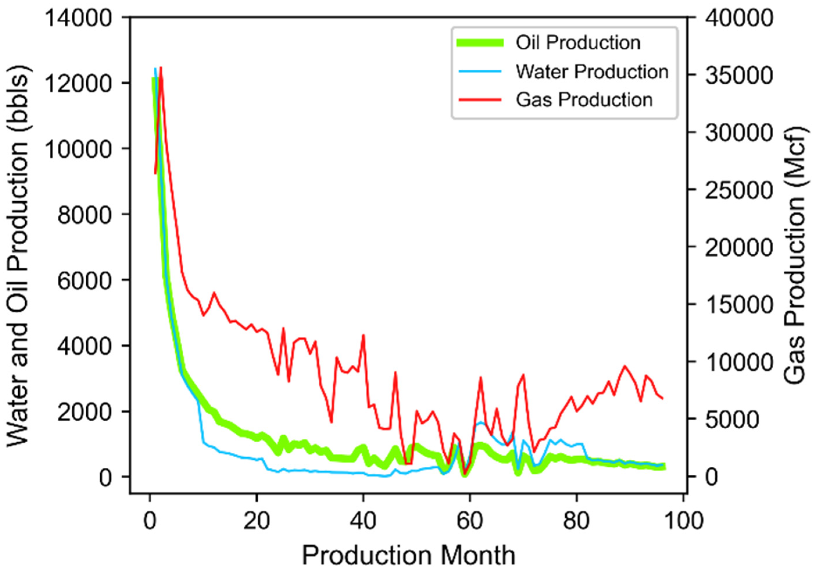
Figure 1. Example of oil, water, and natural gas production data for a horizontal well in northern Reagan County, Texas producing from Wolfcamp A and placed at a total vertical depth of 7713 feet below ground surface. Timeseries fluid data was acquired from vendor Drilling/Enverus [48].
Processes 10 00740 g001
Figure 3. Distribution of static features for each well in the study dataset.
Processes 10 00740 g003
Figure 5. Example schematic of an LSTM cell. Figure concept compiled from concepts presented in Kwak & Hui [131], Olah [132], and Poornima & Pushpalatha [133].
Processes 10 00740 g005
Figure 6. Elbow diagrams from k-means clustering analysis. The top figure (A) represents the total within-cluster sum of squared errors based on the number of clusters evaluated. The lower figure (B) shows the resulting Hartigan’s Index as a function of the numbers of clusters evaluated.
Processes 10 00740 g006
Figure 7. Well data demarcated by color corresponding to one of the 18 clusters (labeled 0–17 based on Python’s zero-based indexing). The top (A) is a three-dimensional representation of well data location which features placement along burial depth. The bottom (B) is a top-down depiction featuring well location by latitude and longitude coordinates only.
Processes 10 00740 g007
Figure 8. Box-and-whisker plots of Arps decline curve attributes calculated for wells within each cluster; including (A) initial oil production, (B) initial decline, and (C) b-factor. Boxes extends from the 25th to 75th quantile values of the data. A line occurs at the median (50th quantile). Green triangles occur at the mean value. Whiskers extend to the minimum and maximum values of the data absent outliers.
Processes 10 00740 g008aProcesses 10 00740 g008b
Figure 9. Learning curves for the joint associated fluid production model over training epochs.
Processes 10 00740 g009
Figure 10. Parity plots of model performance comparing predicted values for monthly gas (A) or water (C) against actual values (i.e., observations) for wells in the test dataset. Additionally, the density of data within plot area pixels is provided for gas (B) and water (D). Density plots zoom to focus on the 0 to 80,000 bbls or Mcf fluid volume range where the majority of test data occurs.
Processes 10 00740 g010
Figure 12. Stacked (left y-axis) and cumulative (right y-axis) histograms of well counts within the study dataset based on the production timeframe for each well.
Processes 10 00740 g012
Figure 13. Gas and water prediction forecast using the joint associated fluid production model leveraging oil forecast outlooks generated from the Arps model.
Processes 10 00740 g013
Figure 14. Oil, water, and gas production volumes under three different development scenarios for the Midland Basin. Each scenario assumes 1842 new wells drilled and completed.
Processes 10 00740 g014
Table 2. Statistical summary of the study dataset features evaluated.
Dataset FeaturesData GroupStaticDynamicMeanMedianStandard Deviation
Monthly Oil (bbls)Well Performance Attributes X486324296448
Monthly Gas (Mcf) 1 X12,500790613,846
Monthly Water (bbls) X8510357213,496
Top 12 Months Gas (Mcf)X 251,286207,532182,648
Top 12 Months Oil (bbls)X 124,320114,31470,210
Top 12 Months Water (bbls)X 226,856197,664157,721
EUR Gas (MMcf)X 1,732,4701,171,6821,722,215
EUR Oil (bbls)X 449,302380,333326,663
Initial Oil Production (bbls) 2Decline Curve AttributesX 20,80719,67511,593
Initial Decline (fraction/month)X 0.350.360.13
b-factorX 1.21.00.2
Timestep Cumulative (months) X25.32118.8
Perforation Length (foot)Well Completion AttributesX 848083021959
Proppant per foot (lbs)X 17321718548
Water per foot (bbls)X 434414
Additive per foot (bbls)X 2.92.42.4
Azimuth (degrees) 3X 1661638
Nearest Well Distance (feet)X 438231838
Percent in Zone (percent)X 9710010
True Vertical Depth (feet)Spatial and
Reservoir
Attributes
X 85718828993
Thickness (feet)X 460415188
Surface Hole Latitude (degrees)X 31.825331.79710.4093
Surface Hole Longitude (degrees)X −101.7740−101.83460.3204
1 Mcf = thousand cubic feet. 2 DrillingInfo/Enverus quantifies initial oil production as the cumulative production volume observed during a given well’s first full month of production [48]. 3 All wellbore azimuth trajectories based on true north = 0 degrees.
Table 3. Summary of network architecture for the joint associated fluid production model.
Layer TypeActivationOutput ShapeTrainable Parameters
MaskingNot Applicable(None, 1, 24)0
LSTMSigmoid(None, 1, 48)14,016
LSTMSigmoid(None, 1, 96)55,680
DenseSigmoid(None, 1, 96)9312
DenseSigmoid(None, 1, 48)4656
DenseLinear(None, 1, 2)194
Table 4. Summary of feature inclusion for the various dataset aggregates. Each feature is demarcated for inclusion into the associated dataset aggregates as an input feature (x) or a response feature (y).
Dataset FeaturesData GroupFeature SelectionClusteringJoint
Time Series Prediction
Monthly Oil (bbls) (t through t − 4)Well Performance
Attributes
x
Monthly Gas (Mcf) (t through t − 4) y
Monthly Water (bbls) (t through t − 4) y
Top 12 Months Gas (Mcf)yx
Top 12 Months Oil (bbls)xx
Top 12 Months Water (bbls)yx
EUR Gas (MMcf)
EUR Oil (bbls)
Initial Oil Production (bbls)Decline Curve
Attributes
x
Initial Decline (fraction/month) x
b-factor x
Timestep Cumulative (months) x
Perforation Length (foot)Well Completion
Attributes
xxx
Proppant per foot (lbs)xxx
Water per foot (bbls)xxx
Additive per foot (bbls)xxx
Azimuth (degrees)xxx
Nearest Well Distance (feet)xxx
Percent in Zone (percent)x
True Vertical Depth (feet)Spatial and Reservoir
Attributes
xxx
Thickness (feet)xxx
Surface Hole Latitude (degrees)xxx
Surface Hole Longitude (degrees)xxx
Wolfcamp (yes/no)x
Spraberry/Dean (yes/no)x
Table 5. Model results for prediction on the training and test dataset.
Predicted ValueTraining DataTest Data
R2MSERMSER2MSERMSE
Monthly Gas (Mcf)0.9307.63 × 10627620.9317.54 × 1062746
Monthly Water (bbls)0.9146.72 × 10625930.8997.35 × 1062710
Joint Prediction (Monthly Water and Gas)0.9227.17 × 10626790.9157.44 × 1062728
Table 6. Inventory of first year and cumulative five-year production estimates for a hypothetical representative well within each Midland Basin Well Cluster.
Response FeatureOutlook YearMidland Basin Well Cluster Number: 0 through 8
012345678
Cumulative Oil (Mbbls)1st year7711114710038181868273
5-years15428227518374346156169145
Cumulative Gas (Bcf)1st year0.160.200.250.150.120.270.250.130.22
5-years0.290.580.620.230.230.600.760.210.79
Cumulative Water (Mbbls)1st year154230268181102304200162182
5-years289587545347175659358324328
Response FeatureOutlook YearMidland Basin Well Cluster Number: 9 through 17
91011121314151617
Cumulative Oil (Mbbls)1st year14189808716013512923750
5-years28117316816732826527946591
Cumulative Gas (Bcf)1st year0.260.140.120.150.310.220.220.340.12
5-years0.570.190.160.270.910.500.450.850.27
Cumulative Water (Mbbls)1st year271185170171306249265373111
5-years574364287332684515621879178
Table 7. Summary of the highest and lowest predicted production totals and associated cluster groups.
MetricOil ProductionNatural Gas
Production
Water ProductionGas-to-OilWater-to-Oil
MbblsClusterBcfClusterMbblsClusterBcf/MbblClusterMbbl/MbblCluster
Highest 1st year237160.3416377160.0014161.5916
Highest 5 years465160.9113879160.0020111.8911
Lowest 1st year3840.124 and 1110240.003242.684
Lowest 5 years7440.161117540.002282.364
Publisher’s Note: MDPI stays neutral with regard to jurisdictional claims in published maps and institutional affiliations.