Hot-Wire Investigation of Turbulence Topology behind Blades at Different Shape Qualities

Abstract

The scope of this paper is to perform a detailed experimental investigation of the shape error effect on the turbulence evolution behind NACA 64-618 airfoil. This airfoil is 3D-printed with predefined typical shape inaccuracies. A high-precision optical 3D scanner was used to assess the shape and surface quality of the manufactured models. The turbulent flow was studied using hot-wire anemometry. The developed force balance device was provided to measure the aerodynamic characteristics of the airfoil. Experimental studies were carried out for three angles of attack, $+{10}^{\circ }$, $0^{\circ }$, $-{10}^{\circ }$, and different chord-based Reynolds numbers from $5.3\times {10}^4$ to $2.1\times {10}^5$. The obtained results show that the blunt trailing edge and rough surface decline the aerodynamic performance of the blades. In addition, the experimental results revealed a strong sensitivity of the Taylor microscale Reynolds number to the type of shape inaccuracy, especially at $Re\approx 1.7\times {10}^5$. We also discuss the evolution of the Reynolds stress components, the degree of flow anisotropy, and the power spectrum distributions depending on the airfoil inaccuracies.

1. Introduction

The behavior of the flow around a bluff body is a nonlinear problem. One of the consequences of the nonlinearity is an unpredictable sensitivity on boundary conditions deviations, however small they may be. The scale of possible reactions to some small geometric perturbations ranges from almost zero effect to a complex change of the flow structure. That makes it difficult to predict the turbulence evolution. The situation could be characterized as one of passive low control, however unwanted. Even small variations of the boundary conditions—shape and roughness of the airfoil—could cause important changes in aerodynamic characteristics.

In recent years, a large number of papers were devoted to aerodynamic characteristics of an airfoil. The researchers focused on the spatial and spectral investigation of turbulence parameters. Some of them, based on experiments, were studying in detail the physical aspects of the turbulence formation behind the bladed rotor. Others explored the structure of flow around an isolated airfoil. However, nearly ideal shape of the airfoil is considered for the experimental research with sharp trailing edge and smooth surface, which is far from real application. The airfoil profiles are designed with “absolutely sharp” trailing edge very often, this means that the thickness of the trailing edge approximates zero. This condition could be relatively well approximated in the case of laboratory model, but definitely not in the case of a real machine. The reasons could be technology of manufacturing, strength design or erosion, to mention the most important. The effect of the resulting geometry modifications on an airfoil aerodynamic characteristics was not studied systematically in the available literature. The presented paper is a contribution towards filling this gap.

The flow behind blades has been studied extensively in past. For example, the papers in [1,2] show experimental results related to the investigation of turbulence and secondary flows at the outlet of an axial turbomachine. The obtained results contain valuable information about the transport of turbulent structures in unstable, deterministic flow patterns. The authors suggest that turbulence generated at the shear layers is anisotropic. Moreover, they established links between the blade pitch angle and the turbulent intensity.

Meanwhile, other papers [3,4] show that higher turbulence intensity or Reynolds number significantly improve the aerodynamic performance of the airfoil. This effect can be observed for all angles of attack. In addition, the intensity of turbulence strongly affects the boundary layer characteristics [5]. This plays an important role in the formation of flow behind a streamlined body, therefore, many researchers have focused on this issue. Moreover, the formation of a boundary layer is nontrivial and depends on the surface quality and geometry of a body [6]. The profile of an airfoil can be either symmetrical or asymmetrical. The work in [7], presents an investigation of turbulence quantities in the boundary layer and near-wake of the symmetric airfoil at different angles of attack. The authors demonstrated how a modification of the boundary layer affects the development of the wake. Some similar studies, but for the asymmetric airfoil, are performed in [8]. The authors describe the structure of the turbulent flow in the wake and boundary layer regions in detail. In addition, they define the transition range between instability and free stream zone based on spectral and anisotropy analyses. Generally, the pressure gradients are different across asymmetric and symmetric airfoils. Accordingly, under increasing turbulence intensity, for asymmetric profile, the maximum lift is reduced by 30%. Whereas, this characteristic for a symmetrical profile, on the contrary, increases by 5% [9].

Nowadays, many researchers also pay attention to the quality of an airfoil surface. Since even a slight roughness of the streamlined body significantly changes the structure of the wake flow [10], it shifts the transition to turbulence and the separation points. The first fundamental result investigations of this phenomenon are presented in the works in [11,12]. The authors discovered that roughness leads to activation of mixing and turbulent transport processes in the boundary layer. The laminar–turbulent transition of the boundary layer could be accelerated, the bypass mechanism could take place. This causes boundary layer thickening and increasing turbulent diffusion in the generated wake [13,14]. On the other hand, the turbulent boundary layer is more resistive to separation, this effect could render the wake thinner. Moreover, there is a strong dependence between the location of transition inception in separation bubbles and the roughness value of the surface [15]. In addition, the roughness has a strong effect on the general turbulence properties, which results in an increase in turbulence intensity and Reynolds shear stress [16]. This behavior in turn leads to an increased heat-transfer coefficient and friction factor [17]. The results of many experimental studies confirm this pattern. For example, in [18,19,20], the authors investigated how the blade cooling process depends on roughness. As a result, they noted that with micro irregularity, the heat-transfer rate grows significantly.

Moreover, the geometry of the streamlined body is one of the fundamental reasons for the appearance of airfoil self-noise. This is a typical effect of the airfoil interaction with the turbulence produced by the boundary layer [21,22]. Many researchers, using different methods, have investigated this phenomenon [23,24]. Their results show that the airfoil self-noise is significantly dependent on the trailing-edge geometry and quality of the streamlined surface [25,26,27,28].

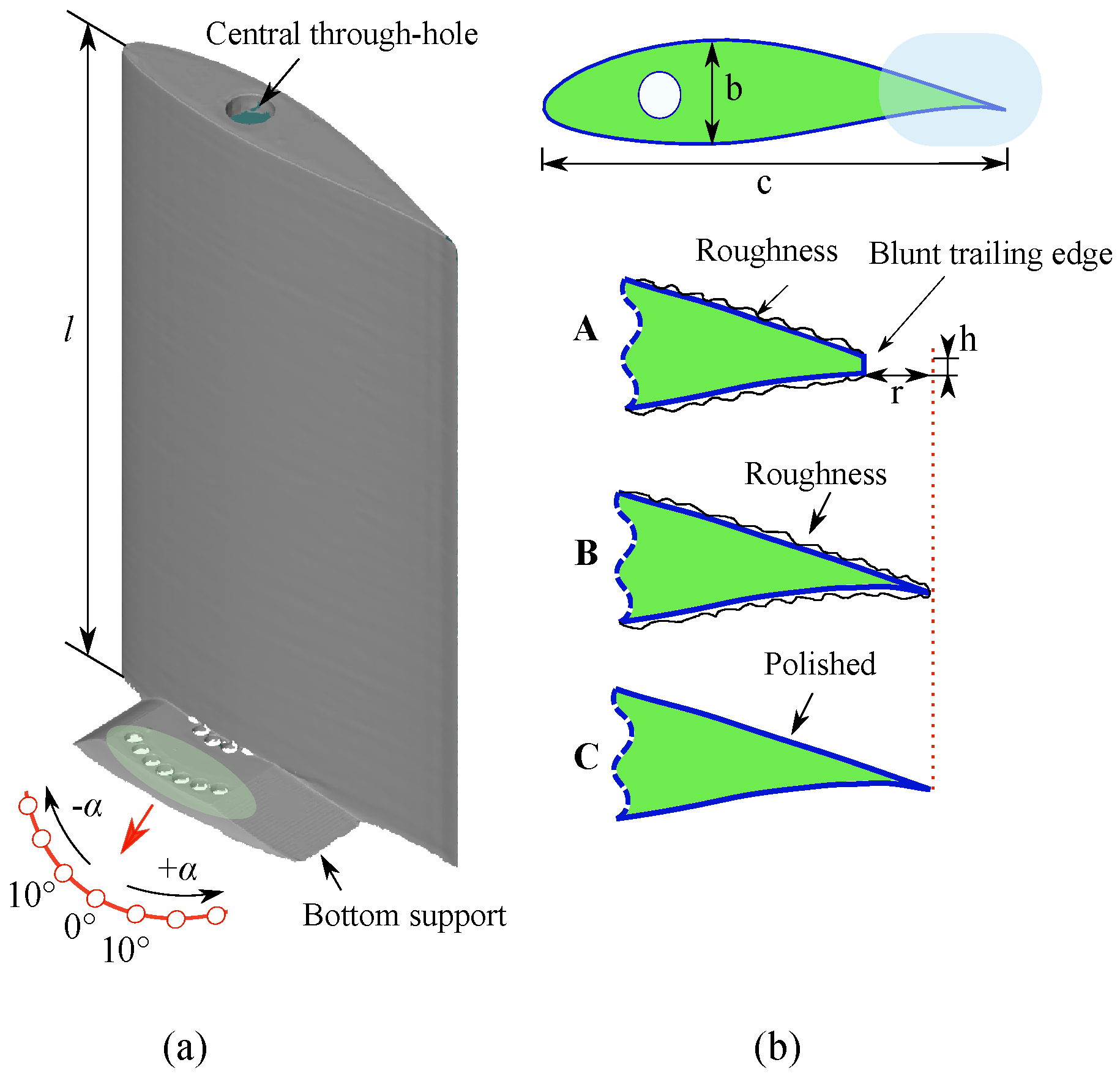
An airfoil is typically defined by its contour by large number of points with exactly defined coordinates. As a rule, the trailing edge is “sharp”, meaning that the thickness of the airfoil at the trailing edge approaches 0. This condition concerns our profile NACA 64-618. The reason for this choice is historical, the Kutta–Joukowski theorem is used for the lift estimate, which requires a sharp trailing edge, see, e.g., ref. [29].

The problem is that the absolutely sharp trailing edge could not be made in practice for technological reasons [30]. Moreover, the size of the airfoil—its chord length—is very different between a real machine and a physical model used during aerodynamic experiments in wind tunnels. The scale could be 1:10, however, the thickness of the trailing edge and roughness of the surface are more or less the same, given by the manufacturing technology. For example, the real thickness of the trailing edge could be about $0.5\mathrm{mm}$, the same for both the model (chord $0.1\mathrm{m}$) and the real application (chord $1\mathrm{m}$). This means that the real chord is shortened by approximately the same factor about $5\mathrm{mm}$ for the model (representing $5\%$ error) and the application (error only $0.5\%$), respectively. This modification definitely has a very different effect on the two cases’ flow-fields around the airfoils. Therefore, the geometry similarity is not maintained in physical modeling very often.

Please note that a rounded trailing edge is not necessarily cost-effective. It is known that the airfoils with blunt trailing edge could show a very good performance [31]. However, the flow-field is completely different, especially in structure and size of the wake, see, e.g., ref. [32,33]. This influences the pressure drag generation directly. This effect will be addressed in our paper in detail for the specific airfoil. However, the conclusions could be considered more general, at least in a qualitative sense.

In general, the flow evolution around an airfoil strongly depends on its geometry. Even the slightest deviation from an original shape leads to different flow quality, which significantly changes the aerodynamic characteristics of blades. Usually, shape inaccuracies can occur during the production or operation of the streamlined body. In the first case, this is due to technological factors in setting up and organizing the production process. Whereas, in the second, it is associated with the corrosion process [34] or depositions on surface. That is especially an issue for offshore wind turbines, where the blades are in a salt fog environment.

As we can see, the general evolution of the flow around an airfoil is strongly dependent on its geometry. Even the slightest deviation from a given shape can lead to different phenomena. The study of this issue is especially important in the production of various streamlined bodies.

That is why, in this paper, we investigate the impact of the most common airfoil shape inaccuracies on the flow structure behind it. The organization of the remaining parts of the paper is as follows. Methodology of experimental investigations and parameters of the measuring devices are given in Section 2. That section describes the procedure of NACA 64-618 airfoil productions and its modifications for the experiment, as well. Then, the results obtained by hot-wire anemometry are presented in Section 3. In particular, we discuss the features of the wake characteristics, Reynolds stress components, and the degree of flow anisotropy according to airfoil shape error, Reynolds number and angle of attack. Moreover, for some measuring points, the power and dissipation spectral distributions are analyzed. Afterwards, the effect of airfoil shape inaccuracies on the structure of turbulence (Section 4) and aerodynamic forces (Section 5) is evaluated. Finally, Section 6 reports the conclusion.

2. Materials and Methods of Research

2.1. Airfoil Configurations

The NACA 64-618 airfoil was chosen for experimental studies. The reason for this is that its geometry demonstrates high-lift, soft-stall characteristics even at low-Reynolds-number flows, in addition to its overall good performance. The original dimensions of the airfoil model are chord length $c=80\mathrm{mm}$, span $l·c^{-1}\approx 1.25$ and thickness $b·c^{-1}\approx 0.18$.

The general view of the airfoil design is presented in Figure 1a. The angle of attack was changed by turning the airfoil relative to its central through-hole. Then, the set position was fixed by mounting holes of the lower support. Each mounting hole changed the value of the angle by ${10}^{\circ }$.

The airfoil was manufactured from polymerized lactic acid (PLA) by 3D-printing technology, using a PRUSA i3 printer. During printing, the nozzle diameter was $0.4\mathrm{mm}$, the height of the printing layer was $0.15\mathrm{mm}$, nozzle temperature and printing speed were 230 ${}^{\circ }$C and $30\mathrm{mm}·{\mathrm{s}}^{-1}$, respectively. Thus, the standard 3D-printing technology was used.

The characteristic of surface roughness is of prime importance for manufacturing an airfoil. It depends on the technology which is used for this purpose. In the case of 3D printing, the surfaces of the formed components have relatively high roughness. Its magnitude strongly depends on the technological parameters of production. Taking into account the results of [35], we can say that the average roughness of the surface at our printing parameters was $Ra\approx 22$ $\mathsf{\mu }$m.

For experimental research, three modifications of the NACA 64-618 airfoil were produced (A, B, C). Each of them simulated certain shape inaccuracies. As shown in Figure 1b, A and B have approximately the same surface roughness of 22 $\mathsf{\mu }$m. The roughness of C was reduced to ≈5 $\mathsf{\mu }$m by P2500 sandpaper. In addition, the chord length of A was ≈3.5% shorter than the others. Whereas, the thickness trailing edge 100 $·h·c^{-1}$ for A, B and C were $0.62\%$, $0.12\%$ and $0.05\%$, respectively.

The 3D noncontact optical scanning system GOM ATOS Core was applied to assess the airfoil shape deviation. Measurement data from this system formed the foundation of three-dimensional quality control of the finished model. Based on them, we calculated the deviation of the actual size of the airfoil profile relative to the original STL file format. As a result, the maximum standard deviation of form for all types of profiles was approximately $\pm 0.15\mathrm{mm}$ (Figure 2). Note a rough error during printing of the product A, fortunately far from the measurement height.

2.2. Wind Tunnels and Auxiliary Equipment

The experimental investigation was conducted in a low-speed open-type wind tunnel at the department of Power System Engineering, University of West Bohemia (Figure 3a) [36]. Its maximum operating velocity is $90\mathrm{m}·{\mathrm{s}}^{-1}$. Additionally, in the entire range of available velocities, the turbulence intensity is less than 0.3%. This feature allows us to accurately estimate turbulence evolution according to the geometry inaccuracies of the airfoil. A radial fan and a $55\mathrm{kW}$ three-phase electric motor are applied to generate the flow. The stable flow is enabled by automated monitoring of the reference pressure of the generated airflow in the tunnel contraction. LabVIEW software was used for experiment control.

The width, height and length of the test section were $0.3\mathrm{m}$, $0.2\mathrm{m}$ and $0.75\mathrm{m}$, respectively. Its bottom and the sides are monoblocks made of extruded transparent polycarbonate. Whereas, the cover of the test section consists of separate segments. That allows the traverse to move along the test section (relative to the x-axis) (Figure 3b). Meanwhile, the traverse rod moves the probe relative to the crosswise y and spanwise z directions (Figure 3c) by using a pair of stepper motors.

2.3. Experimental Setup

The aerodynamic center of the NACA 64-618 airfoil was located at $\Delta z·c^{-1}\approx 1.9$ and $\Delta x·c^{-1}\approx 2.8$. Where $\Delta z$ and $\Delta x$ is the airfoil position relative to the test section. The scheme of the experimental investigation is shown in Figure 4.

Measurements were carried out for three angles of attack $\alpha =+{10}^{\circ }$, $0^{\circ }$, $-{10}^{\circ }$ at different chord-based Reynolds numbers from $5.3\times {10}^4$ to $2.1\times {10}^5$. Accordingly, $\alpha =0^{\circ }$ corresponds to the position when the airfoil chord has the streamwise direction. In this case, the blockage ratio is equal to $2,3\%$, while for the positive and negative angles, it is about $3\%$. According to Pope and Harper [37], for general tests in the wind tunnel, a maximum ratio of model frontal-area to test-section cross-sectional area should not exceed $7.5\%$. At higher values of the blocking effect, a correction method should be used.

The measuring cross-section was located behind the trailing edge at $x·c^{-1}\approx 0.1$, $0.2$, $0.4$, $1.2$ at $y·c^{-1}\approx 1.8$. The width of measuring cross-section ranged from $z·c^{-1}\approx -1.5$ to $1.5$. Note that preliminary investigations indicate that the intensity of turbulence at given coordinates and a whole range of experimental velocities is less than 0.2%. The step $k_z$ between the measuring points at the instability and stability flow region was 3 and $10\mathrm{mm}$, respectively (the methodology of identification can be found in [38]).

3. Results and Discussion

3.1. Measuring Techniques

The constant temperature anemometer was used to study the turbulent structure behind the airfoil. The basic principle of this device is to compensate for the thermal state of the hot wire [39,40]. The Wheatstone Bridge is used to measure the variation of the wire resistance relative to its temperature. In the case of wire cooling, the operating system of the device instantly supplies more energy to the wire. This is necessary to maintain a constant wire temperature. Thus, the power provided to support the system corresponds to the cooling rate and thus to the value of flow velocity passing by the sensor.

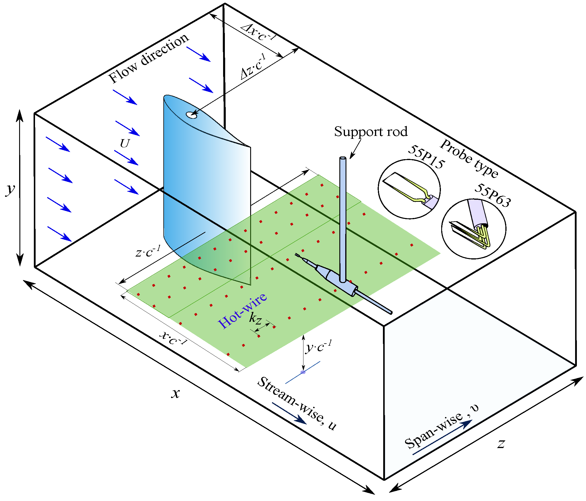
Experimental studies were performed using two types of hot-wire probes. In most cases, we used a miniature wire probe type 55P15. For some measuring points, we also used a miniature X-wire probe 55P63. That allowed us to investigate in more detail the two-dimensional structure of the turbulent flow (u and $\upsilon$ components). The wire probes with tungsten platinum coating have a diameter of 5 $\mathsf{\mu }$m and an active length of $1.25\mathrm{mm}$, while the ends of wire are gilded. The hot-wire signals for all experiments were sampled at $80\mathrm{kHz}$. The filtering of the received signal was applied as well. For the high- and low-pass filter, the frequency was $10\mathrm{Hz}$, and $30\mathrm{kHz}$, respectively. The typical duration of a single point measurement was $10\mathrm{s}$.

The StreamLine system from the company Dantec was applied to calibrate the velocity sensors. This system includes units for generating the flow and supply of dried air. The Collis–Williams law was used to calibrate and estimate the instantaneous flow rate [41,42]. This method is well described in many papers, see, e.g., ref. [43]. The method uses dimensionless description of the sensor cooling law using Reynolds and Nusselt numbers. This approach allows for compensation of pressure and temperature deviations during the experiments.

The precision of measure velocity was determined using the classical methodologies [44,45]. The analysis performed shows that the general uncertainty of the conversion process of the probe electrical signal to the velocity sample is around ±0.5%. This value, in the case of X-wire, is approximately equal for measurements in the streamwise and spanwise directions. Please note that the relative error is related to the maximal velocity, which was in the rage 10–40 m·s${}^{-1}$, depending on the Reynolds number value.

The velocity time series are subjected to statistical data treatment—see, e.g., ref. [46]. LabVIEW and Gnuplot have been used to postprocess the data and produce all the plots presented in the experimental parts of this paper. The Welch method was applied to estimate the power spectral density of a one-dimensional time series. In addition, the solve function was used to determine the calibration constants of the hot-wire probes.

3.2. Wake Topology

A series of experimental studies were performed using the hot-wire probe 55P15. This section presents the analysis of velocity (only the dominant streamwise component u is measured) depending on the airfoil shape inaccuracies ($A,B,C$), angles of attack, Reynolds number and measuring position $x·c^{-1}$.

The experimental program is divided into two measurement campaigns. In the first part, the turbulent flow was investigated close to the trailing edge at different Reynolds numbers. Accordingly, the experiments were conducted at $x·c^{-1}\approx 0.1$ and $Re\approx 5.3\times {10}^4$, $1.07\times {10}^5$, $1.7\times {10}^5$, $2.13\times {10}^5$, what corresponds to 10, 20, 32, $40\mathrm{m}·{\mathrm{s}}^{-1}$. Whereas, the second campaign took place at constant Reynolds number $1.7\times {10}^5\approx 32\mathrm{m}·{\mathrm{s}}^{-1}$ and different measuring positions $x·c^{-1}\approx 0.1$, $0.2$, $0.4$, $1.2$. For better visualization, the obtained data were placed relative to the position of the trailing edge at $\alpha =0^{\circ }$ and normalized by the free-stream velocity U.

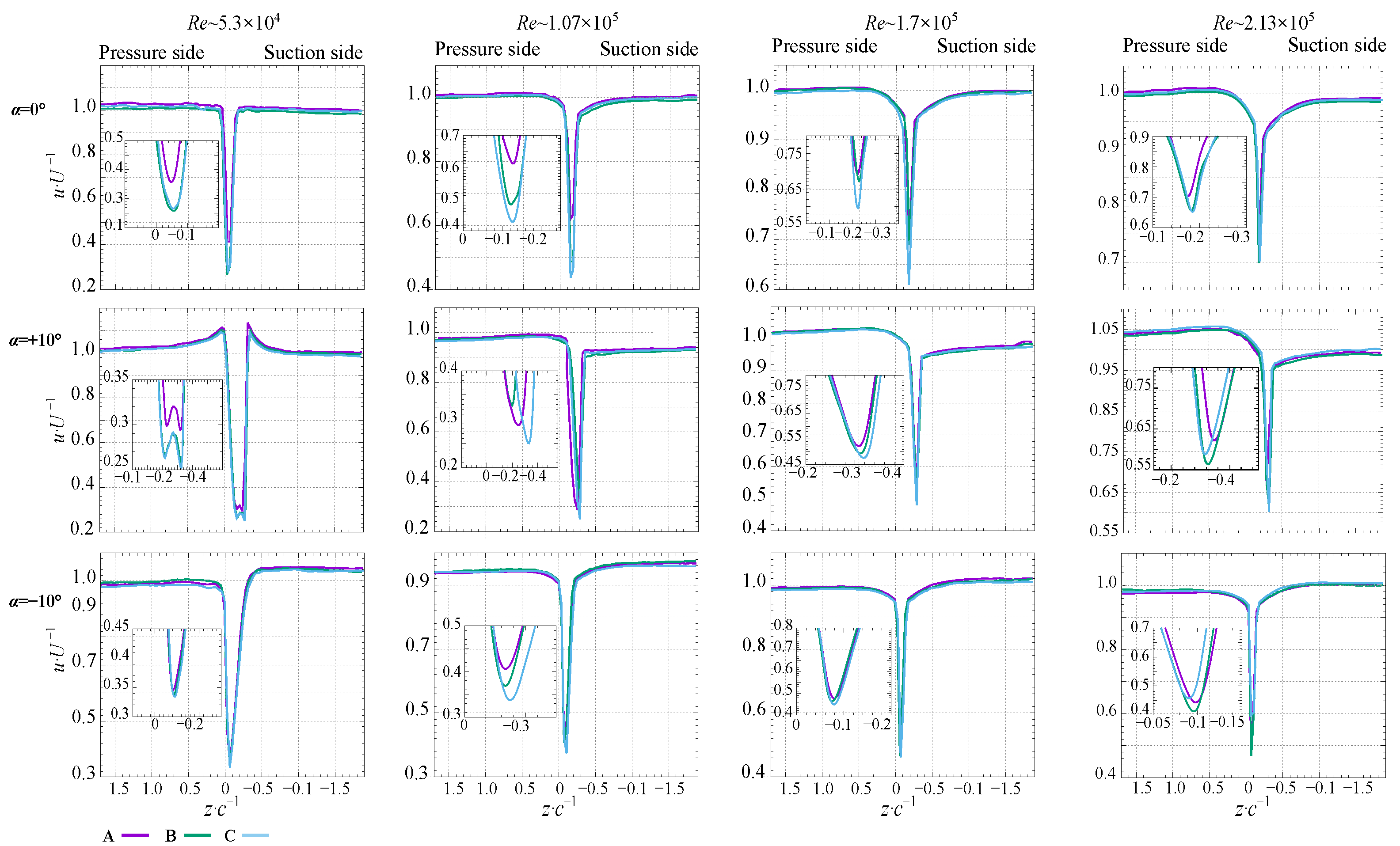
As expected, the obtained results showed a significant effect of the Reynolds number and the angle of attack on the wake characteristics. In particular, as the Reynolds number grows, the depth of the wake increases. The wake width strongly depends on the angle of attack and is the largest at $\alpha =+{10}^{\circ }$. As we can see from Figure 5, the largest and smallest wake velocity deficits are characteristic at the C and A modifications, respectively. Moreover, at zero angle of attack, the difference between them is almost $30\%$. It is caused by that modification A, in contrast to C, has a 4 times greater surface roughness, $1.9\%$ shorter chord length, and $0.62\%$ thicker trailing edge. Thus, according to the experimental data at $\alpha =0^{\circ }$, when the Reynolds number increases to ≈$2.13\times {10}^5$, the wake velocity deficit behind C modification at $\alpha =0^{\circ }$, $-{10}^{\circ }$ and $+{10}^{\circ }$ increases by $2.3$, $2.4$ and $0.8$ times, respectively.

Moreover, at $Re\approx 5.3\times {10}^4$ and the positive angle of attack, the obtained velocity distributions also indicate the presence of a double peak. This phenomenon occurs as a result of the vortices’ interactions with pressure and suction sides of the airfoil [33,47]. Whereas, in other cases, the absence of a double peak means that the flow contains only a single dominant structure. Additionally, the experiments clearly show the displacement of the wake center depending on the angle of attack. This effect occurs due to the difference in flow velocity from different airfoil sides.

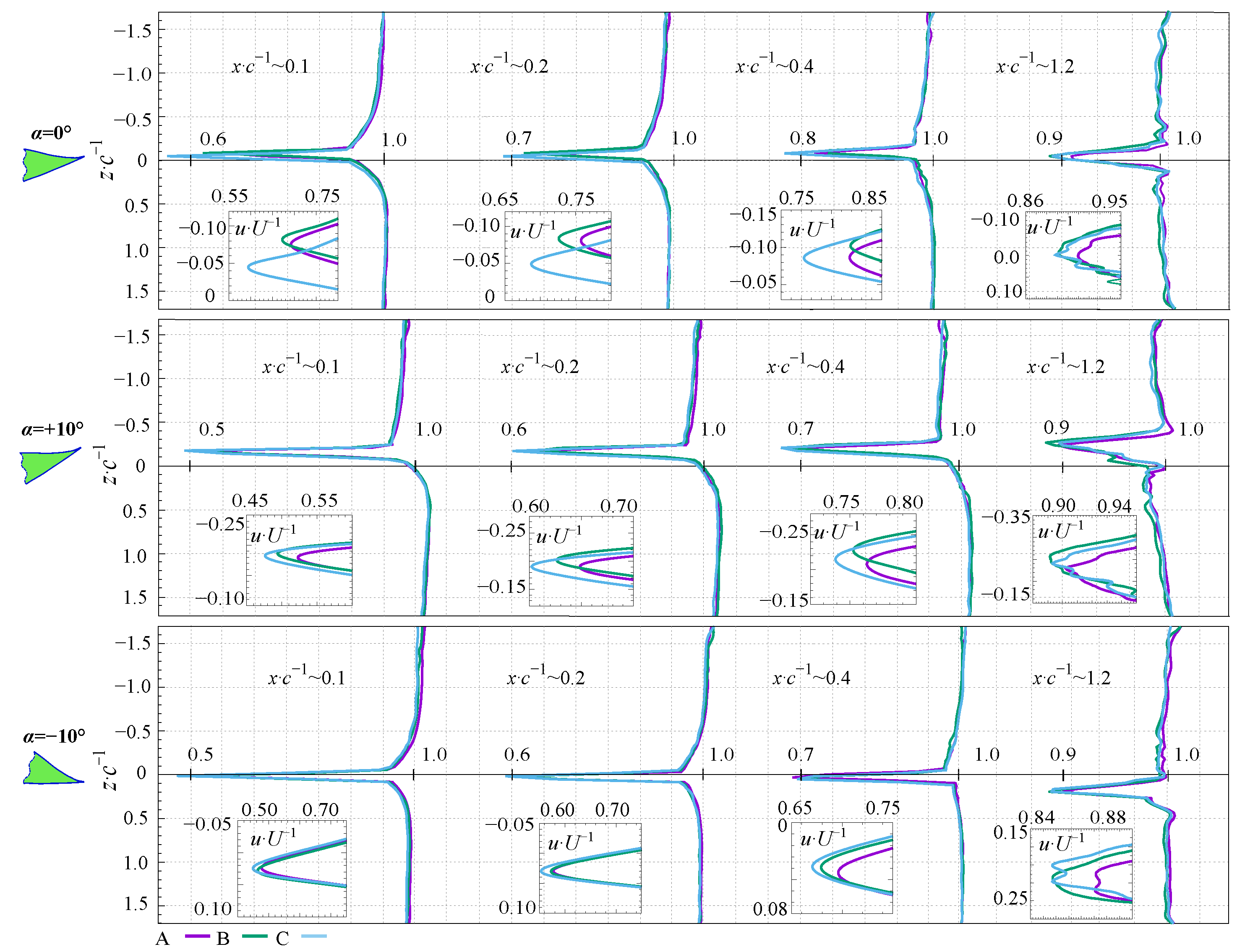
In addition, we investigated the effect of airfoil shape inaccuracies on the wake evolution at increasing distances from the trailing edge. As shown in Figure 6, the wake depth reduces with increasing distance, while the wake width grows as the wake gradually wastes. At the same time, the wake center at $0^{\circ }$ and $+{10}^{\circ }$ shifts to the pressure side while at $-{10}^{\circ }$, it is the contrary. Meanwhile, the absent airfoil shape error leads to a growing velocity deficit. Accordingly, at each measuring cross-section behind the airfoil, the velocity curve for C has a deeper wake than for A and B modifications. In particular, this pattern is clearly visible at zero angle of attack.

3.3. Reynolds Stress Tensor and Degree of Anisotropy

The Reynolds stress tensor was applied to estimate the effect of airfoil inaccuracies on the flow anisotropy. Usually, the Reynolds stress tensor has six independent components that characterize the flow relative to the spatial directions x, z, and y. However, in our case, due to the application of the X-wire probe 55P63, which measures only streamwise and spanwise components, the Reynolds stress tensor was statistically $2D$.

The analysis of flow characteristics took place at two measuring positions $x·c^{-1}\approx 0.2$ and $x·c^{-1}\approx 1.2$ at $Re\approx 1.7\times {10}^5$. For graphical interpretation, the obtained data were normalized by the squared free-stream velocity (Figure 7).

The obtained data indicate that the magnitude and the distribution of the normal stress components strongly depend on the slightest deviations in the airfoil shape. For example, closer to the trailing edge and $\alpha =0^{\circ }$, the value of $\overline{u^{\prime 2}}$ for C modification by $2.3$ and $1.75$ times greater than for A and B, respectively. This explained is due to the variation of the trailing edge and the surface roughness of the airfoil.

With increasing distance to $x·c^{-1}\approx 1.2$, the value of normal stress components decreases significantly. This is especially noticeable at $\alpha =+{10}^{\circ }$, where there is a meaningful dissipation of vortex energy.

In addition, the comparative analysis of the $\overline{u^{\prime 2}}$ and $\overline{{\upsilon }^{\prime 2}}$ distributions reflect the double peaks. This phenomenon is more detail described in papers [7,48,49]. The authors claimed that at a positive angle of attack the double peaks more noticeable. However, in our case, this phenomenon is more visible at the $\alpha =0^{\circ }$ and $\alpha =-{10}^{\circ }$. That is because, for our studies, we used the NACA 64-618 airfoil. This is not only asymmetric but also has some concavity on the pressure side. Thus, the vortices which formed on the pressure and suction sides can propagate in the flow together. Whereas, at $\alpha =+{10}^{\circ }$, the vortices passing from the suction side are increased by vortices from the pressure side. This interaction leads to the formation of a dominant vortex from the suction side in the general flow.

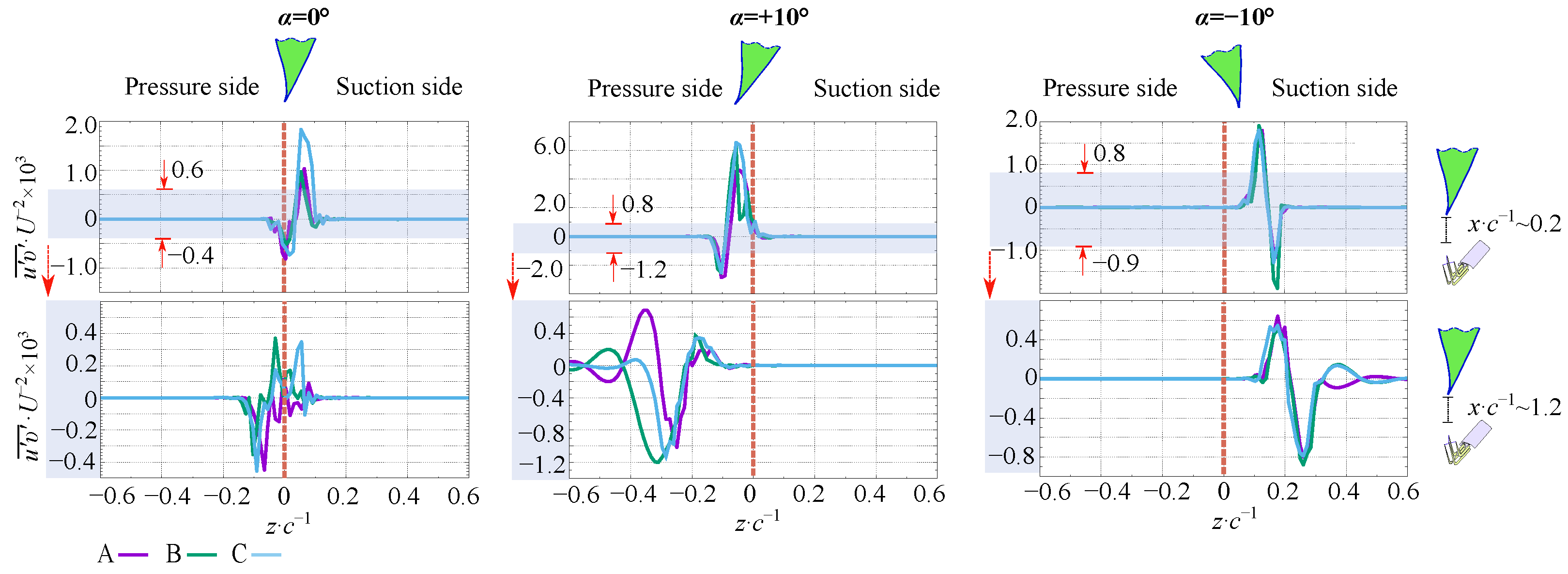
In addition, we also analyzed the effect of airfoil shape inaccuracies on the Reynolds shear stress distributions (Figure 8). Physically, this component is related to the diffusion mechanism for the transport of fluid momentum. Moreover, using the $\overline{{\upsilon }^{\prime }{u}^{\prime }}$ distribution, it is possible to clearly define the region of flow instability where the turbulence structure is anisotropic.

Graphical interpretation of the obtained data shows that, in the perturbation area, a negative value is located directly on the pressure side. This indicates that the turbulence intensity at this location progresses and consequently increases frictional resistance in the mean flow. As a result, turbulence receives energy, while the average flow loses it.

The obtained data show that the largest magnitude of the shear component occurs at the positive angle of attack and closer to the trailing edge. Simultaneously, at $\alpha =0^{\circ }$ and $\alpha =-{10}^{\circ }$ the magnitude of $\overline{{\upsilon }^{\prime }{u}^{\prime }}$ is three times smaller. Note the influence of shape inaccuracies on the obtained distributions observed at $\alpha =0^{\circ }$ and $x·c^{-1}\approx 0.2$. At this angle, the maximum of the shear stress component is $0.5$ times lower for A and B than for C modifications. Whereas, at $\alpha =-{10}^{\circ }$ any effect of inaccuracies almost disappears.

According to the experiments, with increasing distance from the trailing edge, the width of the instability region increases, and its depth declines. This pattern is clearly traced for the A modification. That is due to the presence of additional vortices formed by the blunt trailing edge of the airfoil.

As noted above, the Reynolds stress tensor characterizes the turbulence anisotropy [50,51]. Namely, when the flow fluctuations are statistically uniform in all directions, then the shear stress goes to zero and the normal stresses become equal. Otherwise, at $\overline{u^{\prime 2}}\ne \overline{{\upsilon }^{\prime 2}}$ and $\overline{u^{\prime 2}{\upsilon }^{\prime 2}}\ne 0$, the turbulent flow is anisotropic. To quantify the degree of anisotropy, the Formula (1) could be applied, which represents the ratio of velocity component fluctuations.

$$DA=\overline{u^{\prime 2}}/\overline{{\upsilon }^{\prime 2}},$$

(1)

where $\overline{u^{\prime 2}}$ and $\overline{{\upsilon }^{\prime 2}}$ represent time-averaging value of velocity fluctuations in streamwise and spanwise direction, respectively.

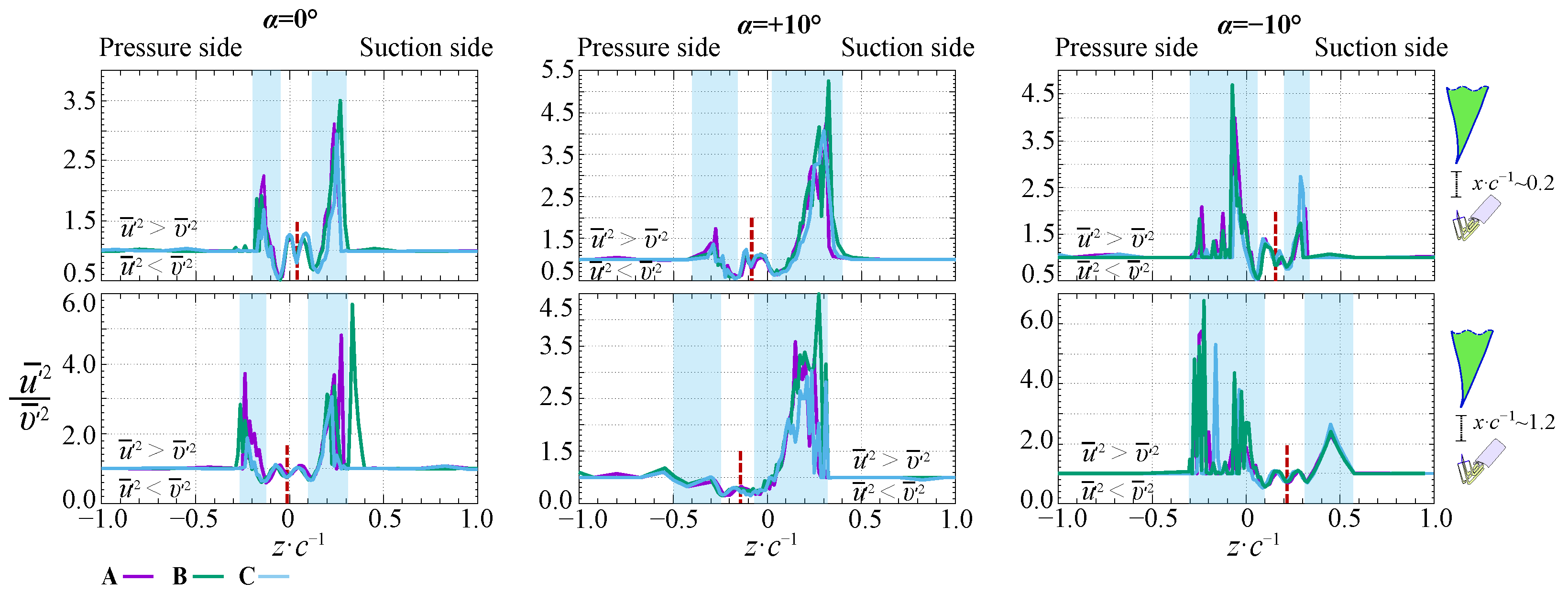
Values of $DA$ greater or smaller than 1 indicate the dominance of the spanwise or streamwise component, respectively. Graphical interpretation of the obtained data at different measuring sections depending on the angle of attack is shown in Figure 9.

As we can see, the width of the anisotropy region is much bigger than the instability region determined by Reynolds stresses components. Comparing these two distributions, we can clearly define the range that characterizes the boundaries of the shear layer (the blue area on Figure 9). In the figure, the instability of the flow is much lower than in the wake. Thus, at some points, even with the smallest difference between the Reynolds stress components, the flow is more anisotropic.

A similar analysis technique is presented in paper [8]. In the study, the authors carefully investigated the flow structure around the FX 63-137 airfoil model. They note that there is some “transit zone” between the free stream and the wake instability region. A feature of this zone is an atypical distribution of power spectral density. Namely, the inertial range has a double slope.

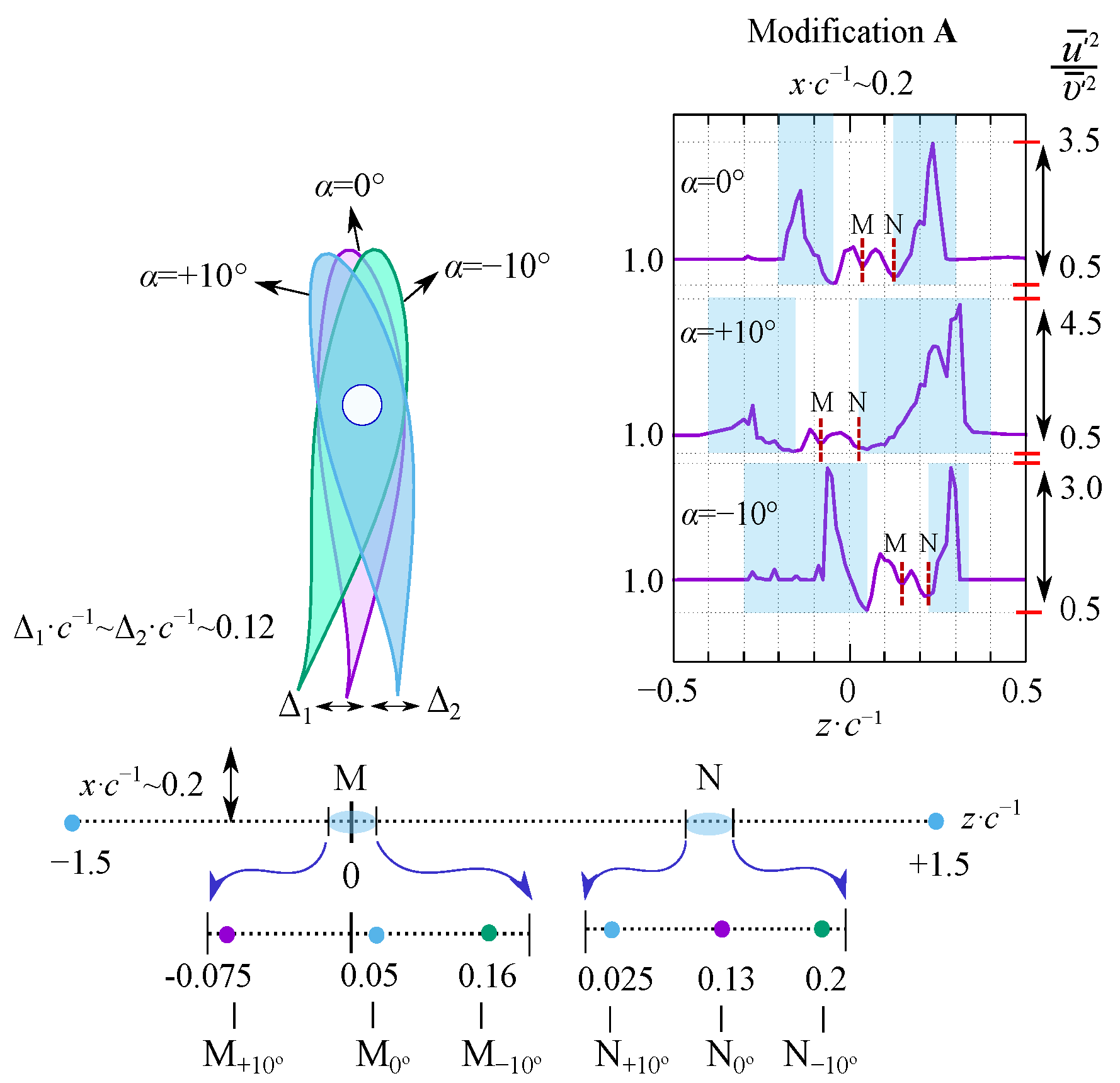
Additionally, as we can see from Figure 9, in the region of Reynolds instability, the DA distribution has a double peak with a local minimum M. This point corresponds to the minimum of the streamwise velocity and the inflection point for the shear stresses distribution. Moreover, the greatest degree of anisotropy observes close to the free stream, where streamwise fluctuations are dominant $\overline{u^{\prime 2}}·\overline{{\upsilon }^{\prime -2}}\approx 3.5$. Whereas, near to the wake, on the contrary, the transverse fluctuation is higher than the longitudinal one $\overline{u^{\prime 2}}·\overline{{\upsilon }^{\prime -2}}\approx 0.5$.

In addition, the areas of the shear layer with the maximum anisotropy values are wider, and their position strongly depends on the angle of attack. For example, at $\alpha =+{10}^{\circ }$ and $\alpha =-{10}^{\circ }$, they are observed from the suction and pressure side, respectively. Additionally, at the negative angle on the pressure side, a significant number of small vortices are generated. These are clearly expressed in the longitudinal direction.

In general, we can conclude that minor manufacturing inaccuracies of the airfoil do not have a significant effect on flow anisotropy. The main factors of this phenomenon are the general geometry of the airfoil and the angle of its attack.

3.4. The Spectral Analysis

The feature of turbulent flow is the presence in its structure of different spatial scales. Power spectral density is widely used to estimate the distribution of energy flux intensity between components of these scales. Physically, it shows the pattern of distribution in the time domain of signal power over the different frequencies.

To spectrally estimate the structure of the turbulent flow, we chose two measurement points, M and N. Accordingly, the first of them is located clearly at the local minimum of the longitudinal velocity component, while the second one is placed on the beginning of the shear layer. The Reynolds number was $Re\approx 1.7\times {10}^5$. It is clear that at different angles of attack, the coordinates of the measuring points M and N will be changed (see Figure 10).

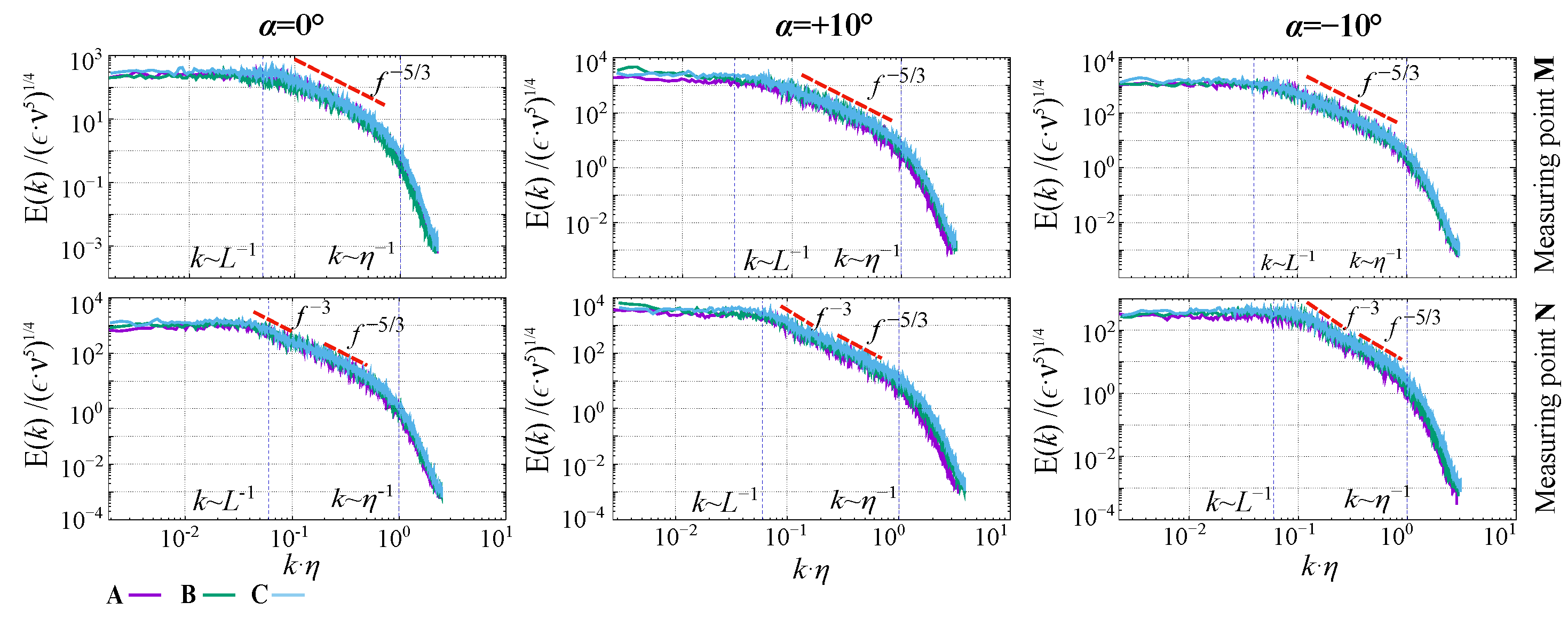
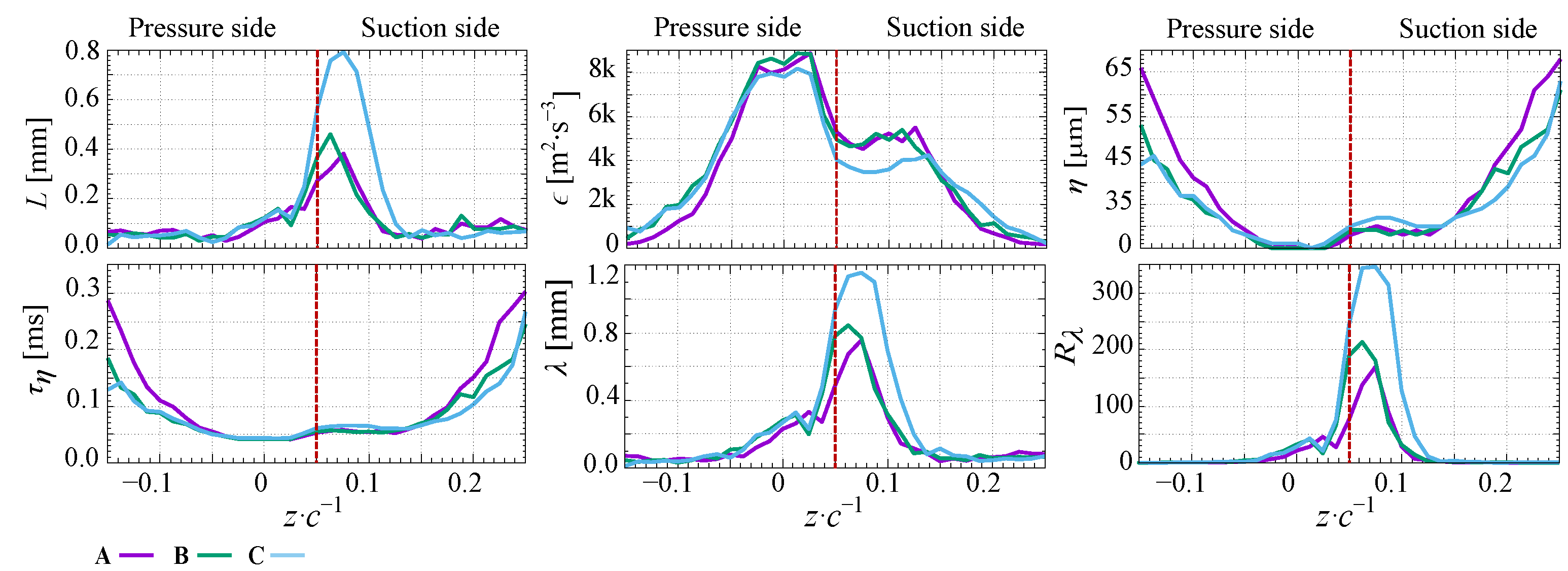
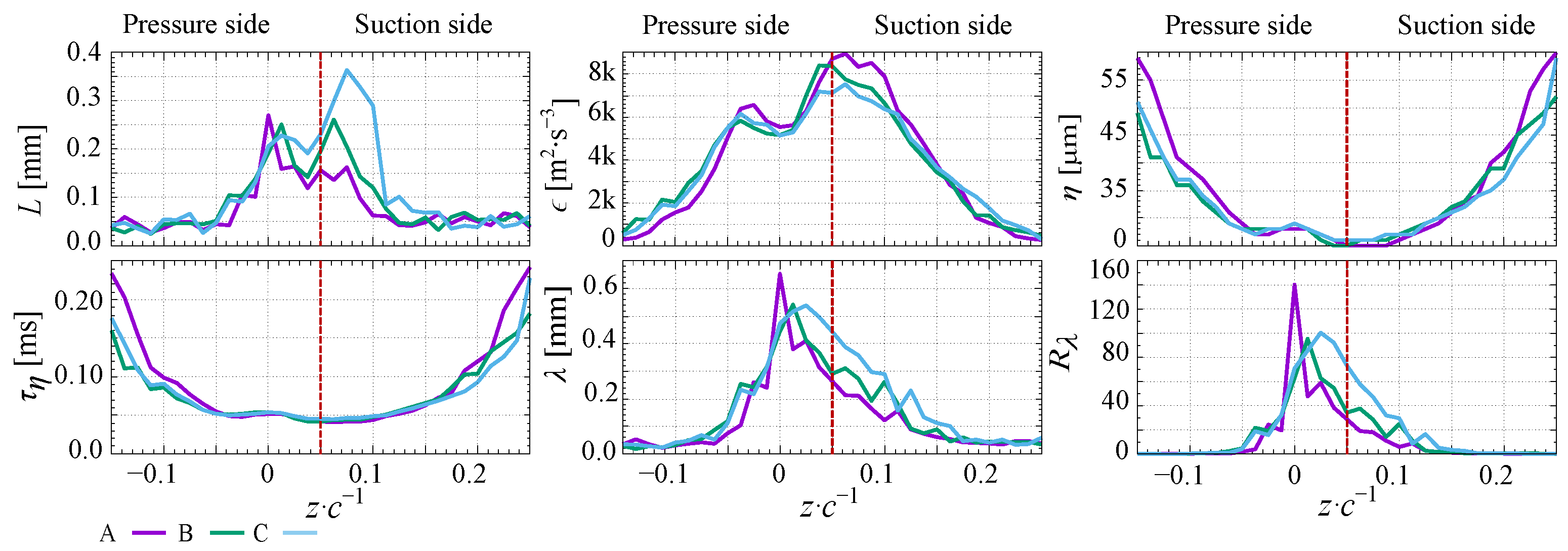
For representing normalized Eulerian power spectral densities of streamwise velocity fluctuations, we used the Kolmogorov nondimensional coordinates (Figure 11). Accordingly, the obtained spectrum was normalized by $E\left(k\right){\left(\eta ·{\nu }^5\right)}^{1/4}$ and the wave number by $\mathit{k}·\eta$, with $\eta$, $ϵ$ and $\nu$ representing dissipation scale, dissipation rate and viscosity, respectively. The method of estimating these parameters is show in Section 4.

As it is known, according to Kolmogorov’s law, the spectral density of turbulence energy decreases with increasing wavenumber. Moreover, in the inertial subrange, the curve has a characteristic slope of $f^{-5/3}$ [52,53]. This pattern is clearly observed for point M, whereby, in longitudinal and transverse directions, the turbulent fluctuations are statistically uniform. Our previous investigations show that at M, the turbulent flow is isotropic. Whereas, the opposite is valid for N in the shear layer. Moreover, this point has a double slope $f^{-3}$ after that of $f^{-5/3}$ in the inertial subrange. This tendency is observed at various airfoil modifications and different angles incidents. Thus, based on the behavior of the energy spectrum, we assume that point N can be determined as the place where the wake instability ends and the shear layer begins.

Additionally, Figure 11 shows that the width of the inertial subrange significantly depends on the angle of attack. Physically, this subrange shows the interval where turbulence kinetic energy is transferred from larger to smaller scales without loss. The largest and smallest width of the inertial subrange is observed at $\alpha =+{10}^{\circ }$ and $\alpha =0^{\circ }$, respectively.

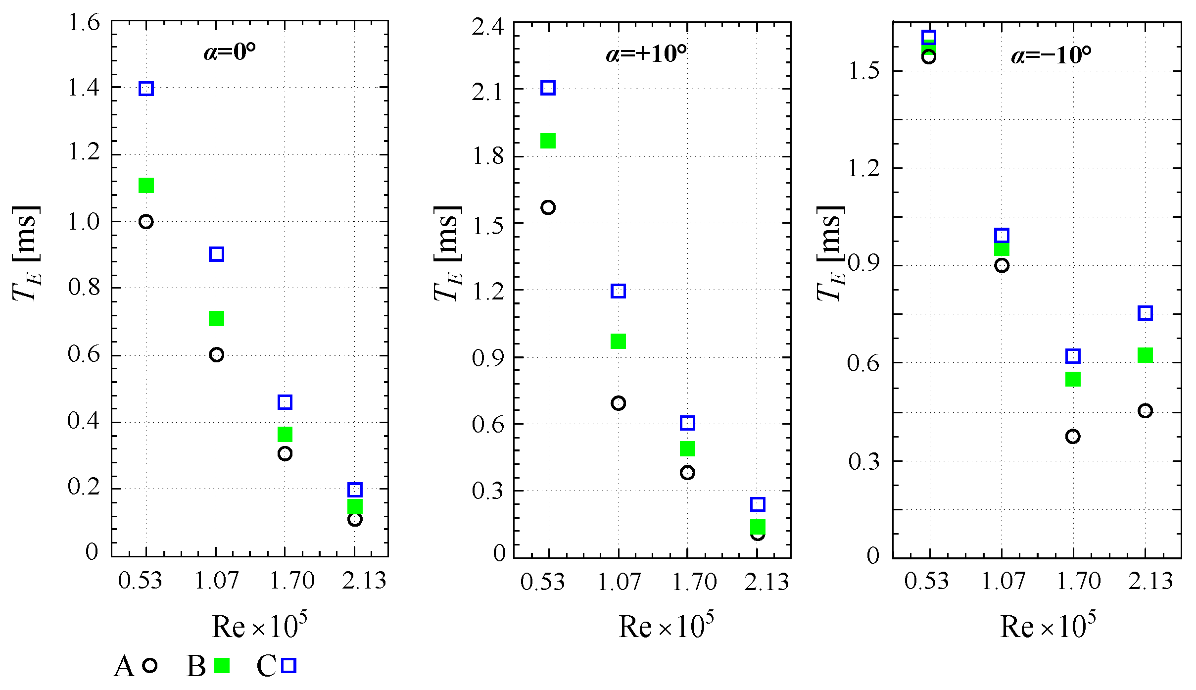
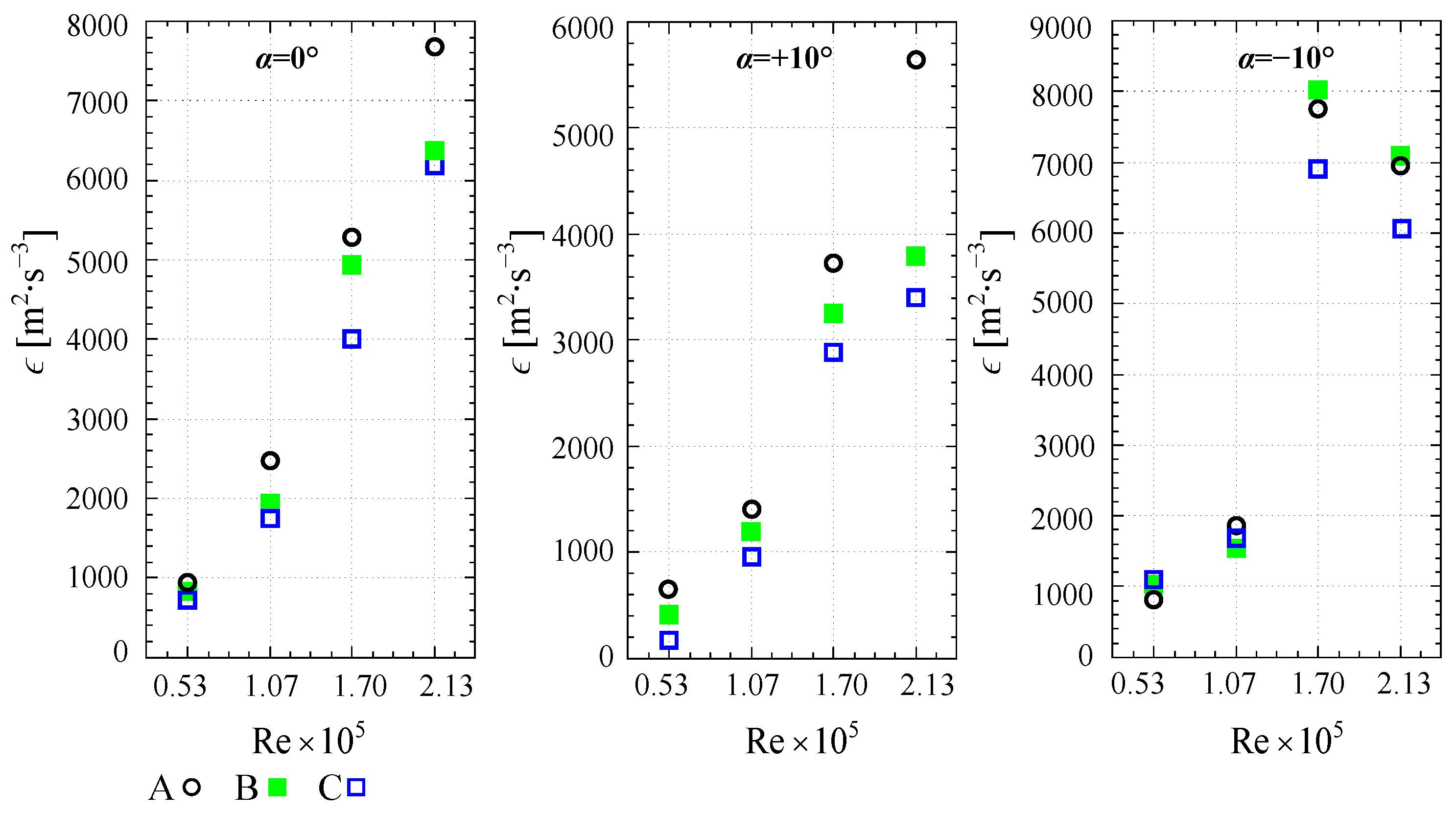
In addition, the dissipation spectrum for the points M and N was evaluated (Figure 12). The dissipation occurs at a high wavenumber, where the smallest vortices dissipate turbulent energy due to viscosity. The magnitude of this phenomenon can be estimated by Formula (2).

$$D\left(k\right)=2\nu k^{2}E\left(k\right)$$

(2)

For non-dimensional coordinates, we used normalization in the form $D\left(k\right)/\eta ·ϵ$ and for wave number $\mathit{k}·\eta$. The data obtained show that at point M, the energy dissipation distribution has a classical form. Namely, the curve in the inertial subrange has a slope of $f^{1/3}$. A similar result for homogeneous isotropic turbulence was obtained by Pope [54]. However, for point N at the beginning of the dissipation range, there is some convexity. After that, the curve has the slope of $f^{1/6}$. This feature is detected only in the place where the shear layer begins. Moreover, the flow characteristic at point N varies greatly depending on the type of shape inaccuracies. In particular, at $\alpha =0^{\circ }$, the value of turbulent kinetic energy for modification C is much greater than A. This pattern is quite logical. In the first case, the airfoil has the best geometry and low surface roughness. That is why the flow receives less resistance. Whereas, for modification A, at turbulence, the flow undergoes a large energy dissipation. However, in any case, we can see that even a small change in the airfoil configuration changes the flow structure.

4. Turbulence Structure Evaluation

Physically, turbulence is an assemblage of discrete perturbations that interact with each other, moving with the flow. Typically, turbulence measurements by hot wire are performed at fixed points, consisting of time history records derived from a sequence of many such perturbations or vortices. The motion inside vortices that are relatively distant from each other (in space or time) usually becomes statistically independent [46,55]. Thus, the measured signal can be considered as random and described in statistical terms. The above-mentioned approach allows finding the time-averaged characteristics of the whole array of vortices. This section presents an analysis of the turbulent structure behind the NACA 64-618 airfoil depending on its shape inaccuracies.

4.1. Turbulence Estimation at the Point

To estimate the structure of turbulence (only in the streamwise direction), we chose the measurement point M. It was located by coordinates $x·c^{-1}\approx 0.2$, $y·c^{-1}\approx 1.8$ and $z·c^{-1}$ from $-0.075$ to $0.16$. For these calculation, $z·c^{-1}$ depended on the angle of attack, according to Figure 10. The experimental Reynolds numbers ranged from $5.3\times {10}^4$ to $2.13\times {10}^5$.

The correlation analysis of time provides a lot of useful information about the mean temporal and spatial scales of turbulent flows [56,57]. Based on the methodology [58], the auto-correlation function $R_{uu}$ can be estimated by

$$R_{uu}=\frac{\overline{u\left(t+\Delta t\right)}·\overline{u\left(t\right)}}{{\sigma }_u^2},$$

(3)

where u is the streamwise velocity component and the overbar is the average value. Additionally, ${\sigma }_u^2$ and $\Delta t$ are the variance of velocity components and the shift time of the measuring signal, respectively.

The obtained distributions of $R_{uu}$ (see Figure 13a) allow us to determine the average lifetime of the largest vortices. Accordingly, the cumulative integral (see Figure 13b) from zero to the point where the value of $R_{uu}$ is equal to zero characterizes the value of the integral time scale $T_E$. This can be represented as follows:

$$T_E={\int }_0^{\infty }{R}_{uu}\left(t^{\prime }\right)d{t}^{\prime }$$

(4)

Graphical interpretation of the integral time scale displayed in Figure 14. The obtained data show the strong dependence of $T_E$ on the Reynolds number and the angle of attack. Accordingly, a quadruple increase in $Re$ leads to a decrease of integral time scale by 10–14 times. Moreover, as the value of $Re$ decreases, the effect of airfoil shape inaccuracy increases. This pattern is valid for zero and positive angles of attack, while at negative angle it has the opposite tendency.

Thus, at $\alpha =0^{\circ }$ and $Re\approx 0.53\times {10}^5$, the presence of a blunt trailing edge and a rough surface (B modification) reduces the value of $T_E$ by 40% compared to the ideal shape of the airfoil (C modification). Whereas, at $\alpha =+{10}^{\circ }$ and the same Reynolds number, this difference is almost 75%. Unexpectedly, the greatest effect of shape error manifested at a negative angle of attack at a high Reynolds number, where inaccuracies in the airfoil geometry reduce the value of $T_E$ almost twice.

It is clear that the integral time scale $T_E$ and integral length scale $L_E$ are interrelated. The last one indicates the average spatial length of the largest vortices and can be determined by the following classical relation:

$$L_E=T_E/{\sigma }_u$$

(5)

where ${\sigma }_u$ is the standard deviation of the streamwise velocity component.

The energy dissipation rate $ϵ$ is one of the most important parameters for assessing the influence of a streamlined body on turbulent flow. It can be estimated from the inertial range dynamics of the turbulence using the second-order longitudinal structure function $S_{uu}^2\left(t\right)$, which, according to Kolmogorov [52] the $S_{uu}^2\left(t\right)$ can be found using the following equation:

$$S_{uu}^2\left(t\right)=2.1{\left(ϵ·t\right)}^{2/3}$$

(6)

where $2.1$ is imperial coefficient [59].

Finally, integrating the plateau of structure function, we can easily determine the value of the dissipation rate $ϵ$ (see Figure 13c). Distributions of dissipation rate depending on the shape inaccuracies in streamwise directions are shown in Figure 15. As expected, the data show a significant effect of the Reynolds number and the angle of attack on the magnitude of the flow dissipation. Meanwhile, the influence of the airfoil shape is also clearly observed. For example, at $\alpha =0^{\circ }$ and $Re\approx 1.7\times {10}^5$ the smallest value $ϵ\approx 4.0\times {10}^3{\mathrm{m}}^2·{\mathrm{s}}^{-3}$ is observed for C modifications, while for B and A, this value is 22% and 30% higher. A similar trend is also present at the positive angle of attack. Moreover, the growing Reynolds number increases the shape impact. Accordingly, at $\alpha =+{10}^{\circ }$ and $Re\approx 2.13\times {10}^5$, for modification A the value of $ϵ$ is 75% higher than for C. However, at $\alpha =-{10}^{\circ }$, there is some difference. Namely, in the range of $Re\approx 1.07\times {10}^5$–$1.7\times {10}^5$, the dissipation rate increases sharply fourfold. Then it begins to decrease slightly.

Once the dissipation rate is known, Taylor microscale $\lambda$, Kolmogorov microscales (length $\eta$ and time ${\tau }_{\eta }$) can be estimated from classical relations:

$$\lambda ={\sigma }_u\sqrt{15\nu /ϵ}$$

(7)

$$\eta ={\left({\nu }^3/ϵ\right)}^{1/4},$$

(8)

$${\tau }_{\eta }={\left(\nu /ϵ\right)}^{1/2}.$$

(9)

Additionally, we evaluated the Reynolds number based on the Taylor microscale by:

$$R_{\lambda }=\left({\sigma }_u·\lambda \right)/\nu ,$$

(10)

As we can see from Figure 16, the value of the Kolmogorov microscale strongly depends on the flow velocity. When the Reynolds number quadruples, the microscale is halved. That is quite logical because with increasing $Re$, the number of small vortices increases significantly. In addition, the effect of shape inaccuracies on the size of the smallest vortices is also clearly visible. That is especially notable at low values of the Reynolds number and positive angle of attack. In these cases, at $Re\approx 0.53\times {10}^5$ , the difference of $\eta$ between A and B cases is almost 22%, while at $Re\approx 2.13\times {10}^5$, it decreases down to 9%.

It should be noted that the Kolmogorov microscale characterizes the size of the smallest vortices which are the source of energy dissipation. This pattern can be observed in the comparative analysis of Figure 15 and Figure 16. Accordingly, as $\eta$ decreases, the value of $ϵ$ increases.

Experimental data also revealed a rather interesting and unexpected distribution of Taylor Reynolds numbers (see Figure 17). Namely, regardless of the angle of attack, at $Re\approx 1.7\times {10}^5$, there is a significant effect of shape errors on the $R_{\lambda }$, while at other velocities, this phenomenon is much smaller. For example, at $\alpha =0^{\circ }$, the presence of a blunt trailing edge and surface roughness in A modification, compared with C, reduces the magnitude of the $R_{\lambda }$ around three times. The effect of shape inaccuracies of modification A is especially evident at $\alpha =+{10}^{\circ }$. In this case, the magnitude of Taylor–Reynolds number for B and C modifications is the same and equal around $R_{\lambda }\approx 470$, while for A, it is three times smaller.

4.2. Characteristics of the Wake Turbulence

The purpose of this subsection is to evaluate the shape effect on the wake turbulence behind airfoil. The methodology of determination of the range of flow instability region is shown in Section 3.1. To estimate the turbulent structure in the streamwise and spanwise directions, we used the methodology described in Section 4.1. Experimental studies were performed at $Re\approx 1.7\times {10}^5$ and $\alpha =0^{\circ }$. The measuring cross-section was located perpendicular to the flow along the z-axis from $-0.15$ to $0.25$ at $x·c^{-1}\approx 0.2$.

Figure 18 and Figure 19 shows the graphical interpretations of turbulence characteristics depending on airfoil shape errors in streamwise and spanwise directions, respectively. According to the results, the greatest shape impact is clearly observed in the wake region. Namely, the values of the integral length scale and Taylor microscale undergo significant changes. This pattern is especially noticeable in the streamwise direction (Figure 18). Thus, the maximum values of the integral length scale are observed at smooth surface and a sharp trailing edge $C-L\approx 0.8\mathrm{mm}$. Whereas, with increasing roughness and the presence of a blunt trailing edge, this value decreases by half. In particular, this occurs for $B-L_E\approx 0.4\mathrm{mm}$ and for $A-L_E\approx 0.32\mathrm{mm}$. Interestingly, the pairwise interaction of these inaccuracies and only the increase in roughness reduces the value of $L_E$ almost equally. This means that surface roughness is the most affected factor which changes the flow structure behind airfoil. Similar trends are present for the Taylor microscale distributions. Accordingly, in the case of B and A, the value of $\lambda$ is the lowest at $0.78\mathrm{mm}$ and $0.75\mathrm{mm}$, respectively. Whereas, for C, this value is almost twice as high.

In addition, the obtained distributions show the logical regularity of the vortex scales location relative to the sides of the airfoil. Namely, the integral length scale $L_E$, in contrast to the Kolmogorov scale $\eta$, is located on the suction side. This is clear because from the pressure side occurs the formation of a significant number of small vortices. That leads to a significant increase in dissipation energy $ϵ$.

Figure 19 shows that in the spanwise direction, the impact of shape errors on turbulence is negligible. However, there is some difference in the distribution of the integral length scale. Namely, this is the presence of a double peak. That indicates dominant vortices, which are formed on both airfoil sides and together propagate along the wake. Moreover, depending on the type of shape errors, their size and location vary. For example, in the presence of a blunt trailing edge and a rough surface, the maximum size of the vortices is observed from the pressure side. Whereas, on the suction side, the dominance vortices can be formed only in the absence of shape inaccuracy.

5. Lift Coefficient Determination

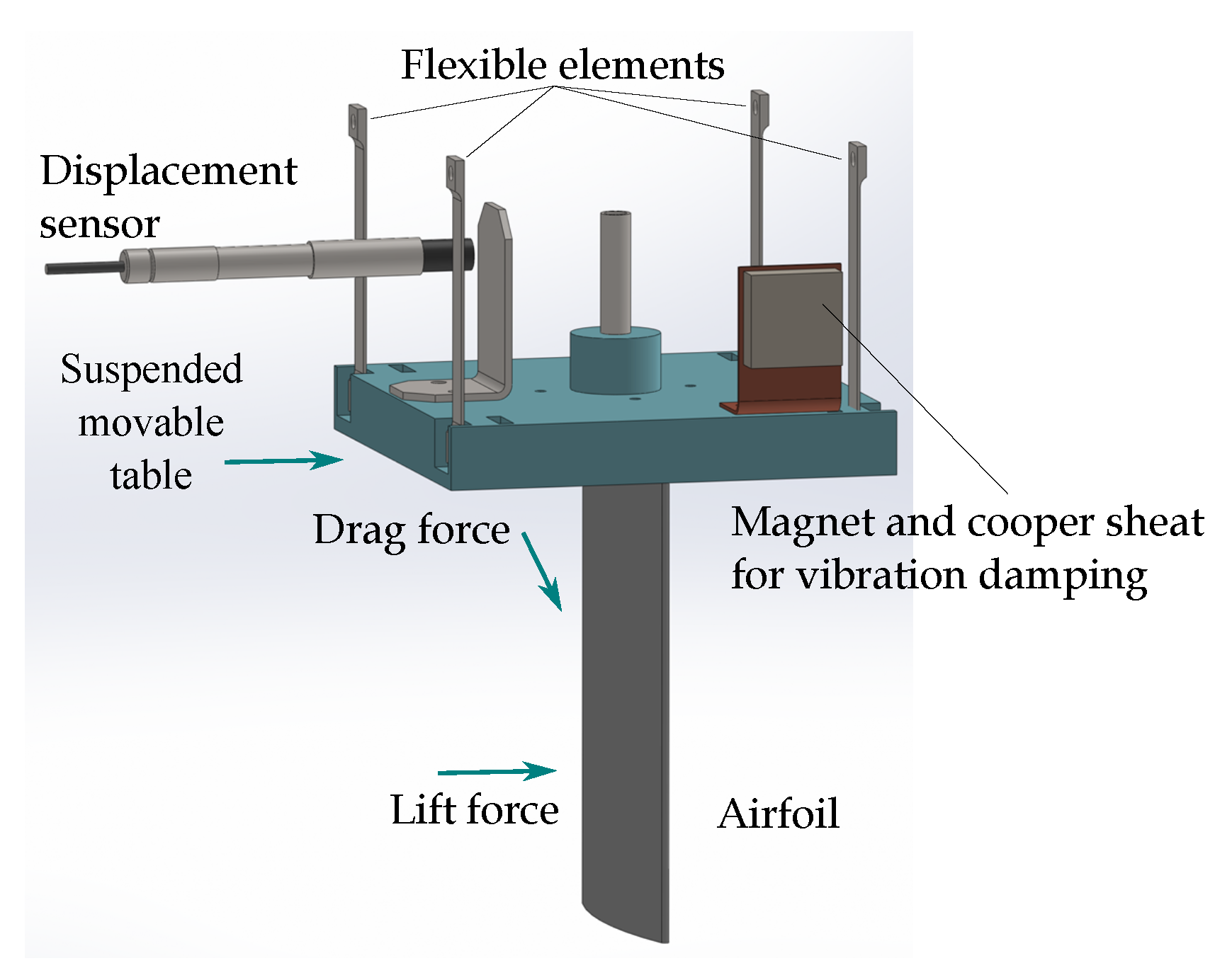
The aerodynamic balance was applied to estimate the effect of shape inaccuracy on the airfoil lift and drag forces [60]. Figure 20 presents a sketch of the developed aerodynamic balance.

The main structural parts of the balance are a resiliently suspended movable table and an eddy current sensor. Meanwhile, the elastic suspension consists of four parallel flexible elements, which have the lowest stiffness in the lift direction of lifting force. The displacement of the table is measured by an eddy current sensor which responds to the distance to the steel target. Unwanted vibrations are dampened by eddy currents in the copper sheet as it moves near to the neodymium super magnet. The sensor output is calibrated by a known force created by using a calibration weight in the lift or drag direction. It should be noted that the measurement error of this device was approximately 1.2%. This error was caused by unwanted airfoil oscillations and to shifting of “zero position” due to low stiffness of the construction parts made of plastic. The uncertainty of the displacement sensor is expected to play a smaller role.

The principle of balance is as follows. The experimental model of the airfoil is fixed to the suspension platform using an aluminum tube and a screw avoiding rotation. The aerodynamic force causes the displacement of the platform, which is recorded using the eddy current sensor. Then, the obtained values of the electric signal using the calibration curves are easily converted into a magnitude of the acting force. 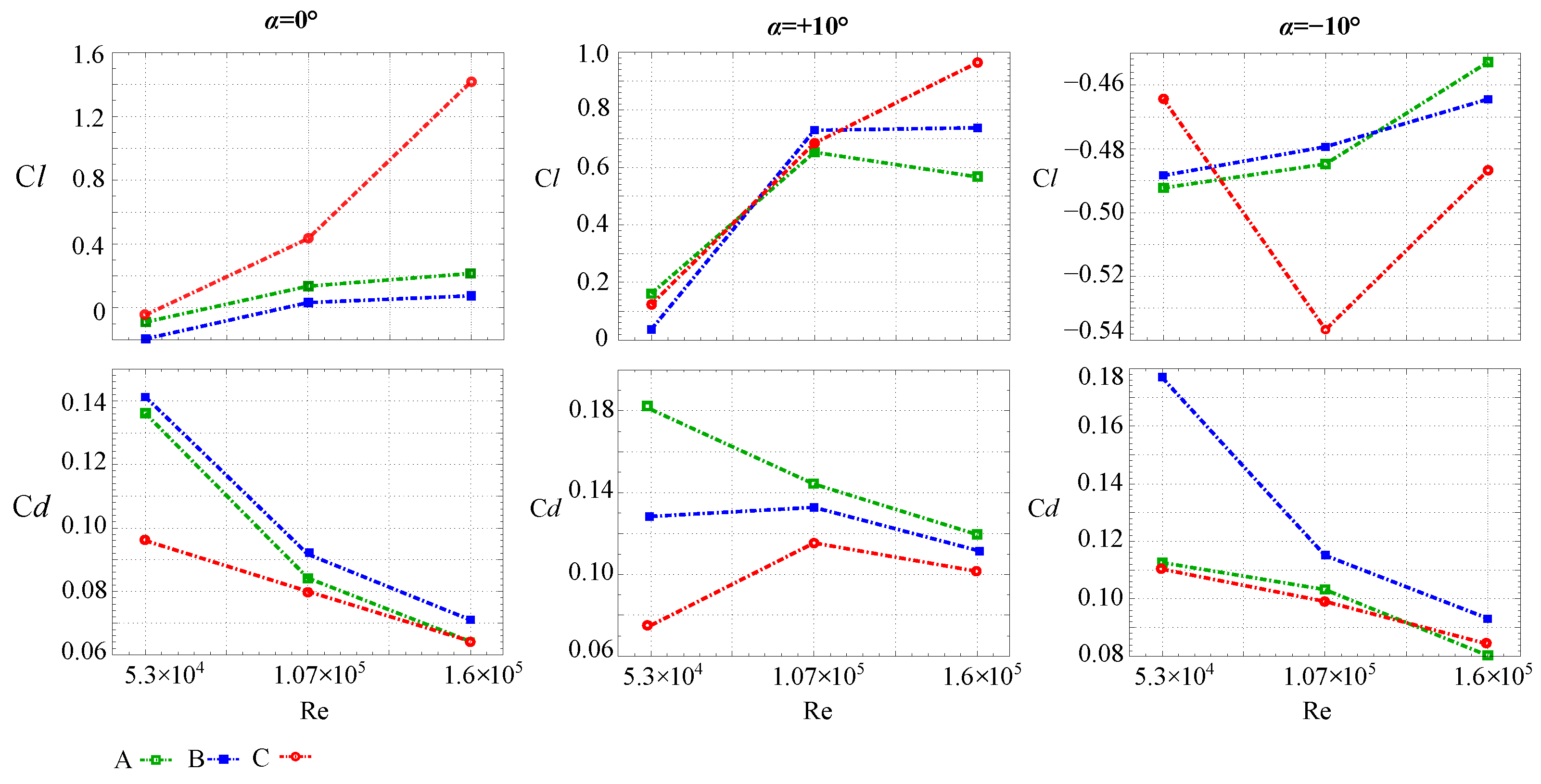Figure 21 presents a graphical interpretation of the lift and drag forces depending on the shape inaccuracy of airfoil and surface roughness.

As expected, the results obtained show that lift characteristics of the airfoil are higher for the best shape configuration. It is especially noticeable at the high Reynolds numbers. For example, at $Re\approx 1.6\times {10}^5$ and $\alpha =0^{\circ }$ the value of $Cl$ for C is 7 times higher than for A and B modifications with rough surface and blunt trailing edge. In addition, the measurements revealed that regardless of the type of airfoil shape error at $\alpha =-{10}^{\circ }$, the values of the lift coefficients are negative. This phenomenon is not new and is typical at low angles of attack [61]. According to the authors of [62], the shape of the separated region, along with the differential growth of boundary layer displacement thickness on the upper and lower surfaces together, introduces an effective negative camber, resulting in a negative circulation around the aerofoil, thereby generating a negative lift.

Additionally, the experimental data suggest that the surface roughness contributes to increasing the drag force compared to the airfoil with a smooth surface. The main cause of this phenomenon is the separation mechanism, which is significantly affected by surface roughness that delays the separation and reduces lift characteristics [63,64].

6. Conclusions

The effect of shape inaccuracies on the flow structure behind NACA 64-618 airfoil was experimentally investigated. According to the data obtained, the roughness has a significant effect on the characteristics of the flow. Thus, at a zero angle of attack, the velocity deficit is $30\%$ higher for a smooth airfoil surface. Generally, the effect of shape error decreases with increasing distance from the trailing edge.

The experimental study also found a large effect of the airfoil shape inaccuracies on the Reynolds stress components. Namely, at zero angle of attack, rough surface and a blunt trailing edge reduce the values of the normal and shear stress components by almost half. However, the analysis of the degree of anisotropy did not detect this effect. In this case, the main impact factors were the general geometry of the airfoil and its angle of attack.

Conducted spectral analysis at the original location of the shear layer detected a double slope of the distribution $f^{-3}$ after that of $f^{-5/3}$. Moreover, at this point, the dissipation spectrum is also characterized by specific behavior displayed by convexity in the inertial range. The obtained distributions indicate that the contribution of wavenumbers to the turbulent kinetic energy is higher for airfoil without shape errors.

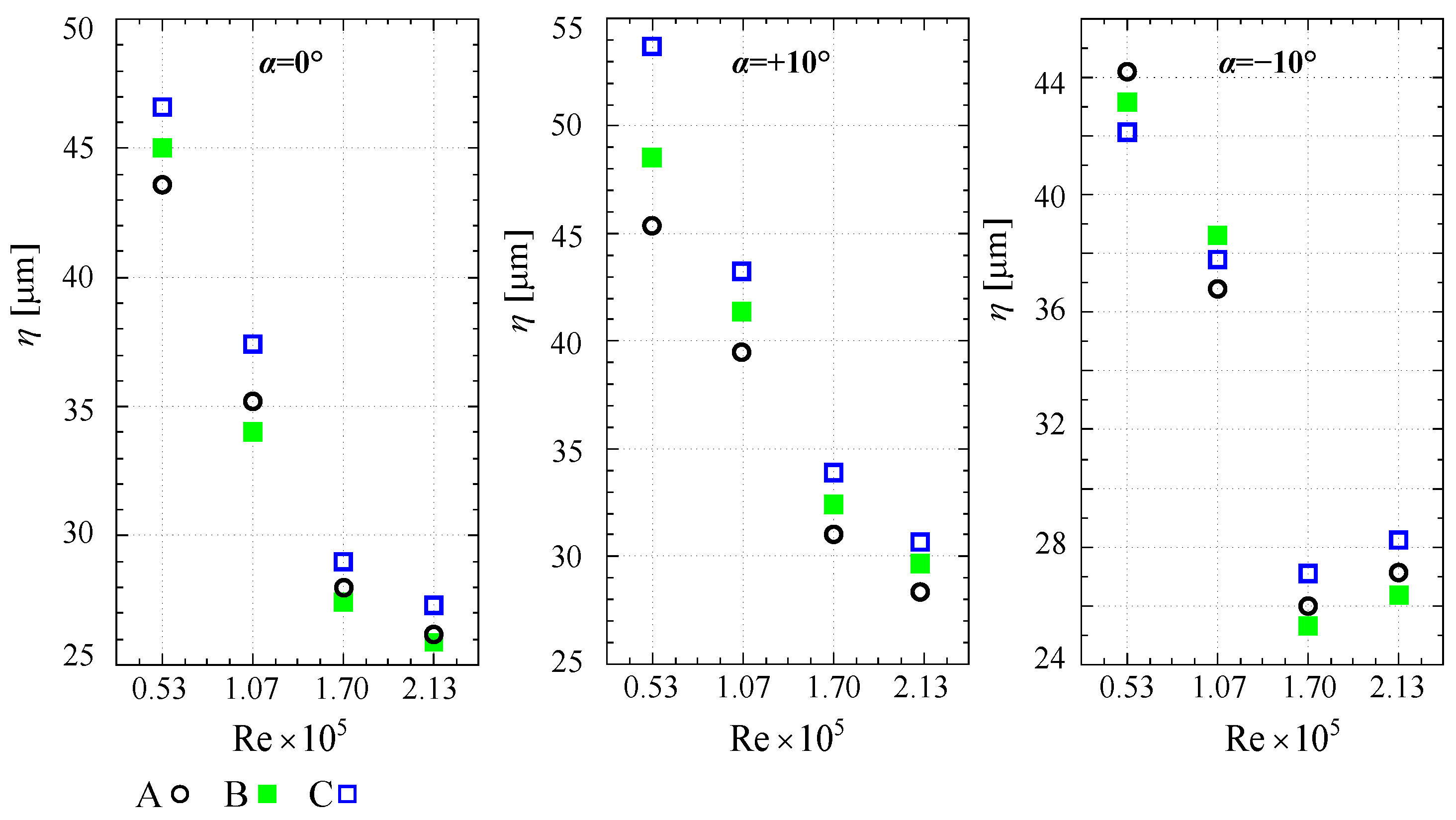
The analysis of turbulent flow structure revealed that the blunt trailing edge and surface roughness increase the value of energy dissipation rate and reduce the Kolmogorov microscale. In particular, the effect of inaccuracies is observed for Taylor microscale Reynolds number at $Re\approx 1.7\times {10}^5$, where it increases almost three times.

Finally, the aerodynamic characteristics of the NACA 64-618 airfoil were estimated. According to the data obtained by aerodynamic balance, the smallest deviation of the airfoil shape leads to an increase in drag and a decrease in lift forces.

The Reynolds and Mach numbers are relatively small in our study, much lower than in any application in a real turbine or a compressor. In future, we intend to extend our study to working with Reynolds numbers at least an order of magnitude higher. The compressibility effect will be considered, as well.

References

1. Oro, J.; Ballesteros-Tajadura, R.; Marigorta, E.; Díaz, K.; Morros, C. Turbulence and secondary flows in an axial flow fan with variable pitch blades. J. Fluids Eng. 2008, 130, 0411011–04110111. [Google Scholar] [CrossRef]
2. Velarde-Suarez, S.; Ballesteros-Tajadura, R.; Santolaria, C.; Blanco-Marigorta, E. Total Unsteadiness Downstream of an Axial Flow Fan With Variable Pitch Blades. J. Fluids Eng. 2002, 124, 280–283. [Google Scholar] [CrossRef]
3. Maldonado, V.; Castillo, L.; Thormann, A.; Meneveau, C. The role of free stream turbulence with large integral scale on the aerodynamic performance of an experimental low Reynolds number S809 wind turbine blade. J. Wind Eng. Ind. Aerodyn. 2015, 142, 246–257. [Google Scholar] [CrossRef]
4. Zhang, Y.; Zhou, Z.; Wang, K.; Li, X. Aerodynamic Characteristics of Different Airfoils under Varied Turbulence Intensities at Low Reynolds Numbers. Appl. Sci. 2020, 10, 1706. [Google Scholar] [CrossRef] [Green Version]
5. Li, S.W.; Wang, S.; Wang, J.P.; Mi, J. Effect of turbulence intensity on airfoil flow: Numerical simulations and experimental measurements. Appl. Math. Mech. 2011, 32, 1029–1038. [Google Scholar] [CrossRef]
6. Winslow, J.; Otsuka, H.; Govindarajan, B.; Chopra, I. Basic Understanding of Airfoil Characteristics at Low Reynolds Numbers (104–105). J. Aircr. 2017, 55, 1–12. [Google Scholar] [CrossRef]
7. Farsimadan, E.; Mokhtarzadeh-Dehghan, M. An experimental study of the turbulence quantities in the boundary layer and near-wake of an airfoil placed at upstream of a 90° bend. Exp. Therm. Fluid Sci. 2010, 34, 979–991. [Google Scholar] [CrossRef]
8. Solís-Gallego, I.; Meana-Fernandez, A.; Oro, J.; Díaz, K.; Velarde-Suarez, S. Turbulence Structure around an Asymmetric High-Lift Airfoil for Different Incidence Angles. J. Appl. Fluid Mech. 2017, 10, 1013–1027. [Google Scholar] [CrossRef]
9. Kay, N.; Richards, P.; Sharma, R. Influence of Turbulence on Cambered and Symmetrical Airfoils at Low Reynolds Numbers. AIAA J. 2019, 58, 1913–1925. [Google Scholar] [CrossRef]
10. Zhang, Q.; Ligrani, P. Wake turbulence structure downstream of a cambered airfoil in transonic flow: Effects of surface roughness and freestream turbulence intensity. Int. J. Rotating Mach. 2006, 2006, 060234. [Google Scholar] [CrossRef] [Green Version]
11. Nikuradse, J. Laws of Flow in Rough Pipes; Tech. Rep. NACA-TM-1292; NACA: Washington, DC, USA, 1933. [Google Scholar]
12. Schlichting, H. Experimental Investigation of the Problem of Surface Roughness; Tech. Rep. NACA-TM-823; NACA: Washington, DC, USA, 1937. [Google Scholar]
13. Zhang, Q.; Lee, S.; Ligrani, P. Effects of Surface Roughness and Turbulence Intensity on the Aerodynamics Losses Produced by a Suction Surface of a Simulated Turbine Airfoil. J. Fluids Eng. 2004, 126, 257–265. [Google Scholar] [CrossRef]
14. Bons, J.; Taylor, R.; McClain, S.; Rivir, R. The Many Faces of Turbine Surface Roughness. J. Turbomach.-Trans. ASME 2001, 123, 739–748. [Google Scholar] [CrossRef]
15. Roberts, S.; Yaras, M. Boundary-Layer Transition Affected by Surface Roughness and Free-Stream Turbulence. J. Fluids Eng. 2005, 127, 449–457. [Google Scholar] [CrossRef]
16. Faruque, A. Roughness Effects on Turbulence Characteristics in an Open Channel Flow; IntechOpen: London, UK, 2019; pp. 1–31. [Google Scholar] [CrossRef] [Green Version]
17. Guo, S.; Lai, C.; Jones, T.; Oldfield, M.; Lock, G.; Rawlinson, A. Influence of Surface Roughness on Heat Transfer and Effectiveness for a Fully Film Cooled Nozzle Guide Vane Measured by Wide Band Liquid Crystals and Direct Heat Flux Gages. J. Turbomach.-Trans. ASME 2000, 122, 709–716. [Google Scholar] [CrossRef]
18. Bogard, D.; Schmidt, D.; Tabbita, M. Characterization and Laboratory Simulation of Turbine Airfoil Surface Roughness and Associated Heat Transfer. J. Turbomach. 1998, 120, 337–342. [Google Scholar] [CrossRef]
19. Bogard, D.; Snook, D.; Kohli, A. Rough Surface Effects on Film Cooling of the Suction Side Surface of a Turbine Vane. In Proceedings of the ASME 2003 International Mechanical Engineering Congress and Exposition, Rome, Italy, 8–13 June 2003; pp. 89–97. [Google Scholar] [CrossRef]
20. Rao, N.; Gumusel, B.; Kavurmacioglu, L. Influence of Casing Roughness on the Aerodynamic Structure of Tip Vortices in an Axial Flow Turbine. In Proceedings of the 51st ASME Turbo Expo Barcelona, Barcelona, Spain, 6–11 May 2006; pp. 1–11. [Google Scholar] [CrossRef] [Green Version]
21. Hardin, J. Airframe Self-Noise: Four Years of Research; Tech. Rep. NASA-TM-X-73908; NACA: Hampton, VI, USA, 1976. [Google Scholar]
22. Brooks, T.; Pope, D.; Marcolini, M. Airfoil Self-Noise and Prediction; Tech. Rep. NASA-RP-1218; NACA: Washington, DC, USA, 1989. [Google Scholar]
23. Williams, J.; Hall, L. Aerodynamic sound generation by turbulent flow in the vicinity of a scattering half plane. J. Fluid Mech. 1970, 40, 657–670. [Google Scholar] [CrossRef]
24. Howe, M. Noise produced by a sawtooth trailing edge. J. Acoust. Soc. Am. 1991, 90, 482–487. [Google Scholar] [CrossRef]
25. Kunze, C. Acoustic and Velocity Measurements in the Flow Past an Airfoil Trailing Edge. Ph.D. Thesis, University of Notre Dame, Notre Dame, IN, USA, 2004. [Google Scholar]
26. Liu, X.; Kamliya Jawahar, H.; Azarpeyvand, M.; Theunissen, R. Wake Development of Airfoils with Serrated Trailing Edges. In Proceedings of the 22nd AIAA/CEAS Aeroacoustics Conference, Lyon, France, 30 May–1 June 2016; pp. 1–21. [Google Scholar] [CrossRef] [Green Version]
27. Jones, L.; Sandberg, R. Acoustic and hydrodynamic analysis of the flow around an aerofoil with trailing-edge serrations. J. Fluid Mech. 2012, 706, 295–322. [Google Scholar] [CrossRef]
28. Vathylakis, A.; Chong, T.; Joseph, P. Poro-Serrated Trailing-Edge Devices for Airfoil Self-Noise Reduction. AIAA J. 2015, 53, 3379–3394. [Google Scholar] [CrossRef] [Green Version]
29. John, D.; Anderson, J. Fundamentals of Aerodynamics, 6th ed.; McGraw-Hill Education: New York, NY, USA, 2017; p. 1154. [Google Scholar]
30. Gupta, V.; Nesterenko, P.; Paull, B. 3D Printing in Chemical Sciences: Applications across Chemistry, 1st ed.; The Royal Society of Chemistry: Cambridge, UK, 2019; p. 264. [Google Scholar]
31. Lee, S.G.; Park, S.J.; Lee, K.S.; Chung, C. Performance prediction of NREL (National Renewable Energy Laboratory) Phase VI blade adopting blunt trailing edge airfoil. Energy 2012, 47, 47–61. [Google Scholar] [CrossRef]
32. Daniel, D.; Vaclav, U.; Yanovych, V. Wake Width: Discussion of Several Methods How to Estimate It by Using Measured Experimental Data. Energies 2021, 14, 4712. [Google Scholar] [CrossRef]
33. Duda, D. How Manufacturing Inaccuracies Affect Vortices in an Airfoil Wake. Proc. Top. Probl. Fluid Mech. 2021, 48–55. [Google Scholar] [CrossRef]
34. Dong, X.; Yuan, T.; Ma, R. Corrosion Mechanism on Offshore Wind Turbine Blade in Salt Fog Environment. Appl. Mech. Mater. 2013, 432, 258–262. [Google Scholar] [CrossRef]
35. Alsoufi, M.; El-Sayed, A. Surface Roughness Quality and Dimensional Accuracy—A Comprehensive Analysis of 100% Infill Printed Parts Fabricated by a Personal/Desktop Cost-Effective FDM 3D Printer. Mater. Sci. Appl. 2018, 9, 11–40. [Google Scholar] [CrossRef] [Green Version]
36. Yanovych, V.; Duda, D.; Horáček, V.; Uruba, V. Research of a wind tunnel parameters by means of cross-section analysis of air flow profiles. AIP Conf. Proc. 2019, 2189, 020024. [Google Scholar] [CrossRef]
37. Barlow, J.B.; Rae, W.H.; Pope, A. Low Speed Wind Tunnel Testing, 3rd ed.; John Wiley and Sons: Hoboken, NJ, USA, 1999; p. 728. [Google Scholar]
38. Yanovych, V.; Duda, D.; Horáček, V.; Uruba, V. Creation of recombination corrective algorithm for research of a wind tunnel parameters. AIP Conf. Proc. 2019, 2118, 030050. [Google Scholar] [CrossRef]
39. Bruun, H. Interpretation of a hot wire signal using a universal calibration law. J. Phys. E Sci. Instrum. 1971, 4, 225–231. [Google Scholar] [CrossRef]
40. Bruun, H. Hot wire data corrections in low and in high turbulence intensity flows. J. Phys. E Sci. Instrum. 1972, 5, 812–818. [Google Scholar] [CrossRef]
41. Nix, A.; Smith, A.; Diller, T.; Ng, W.; Thole, K. High Intensity, Large Length-Scale Freestream Turbulence Generation in a Transonic Turbine Cascade. Am. Soc. Mech. Eng. Int. Gas Turbine Inst. Turbo Expo (Publ.) IGTI 2002, 3, 961–968. [Google Scholar] [CrossRef] [Green Version]
42. King, L.V.; Barnes, H.T. On the convection of heat from small cylinders in a stream of fluid: Determination of the convection constants of small platinum wires, with applications to hot-wire anemometry. Proc. R. Soc. Lond. Ser. A Contain. Pap. A Math. Phys. Character 1914, 90, 563–570. [Google Scholar] [CrossRef] [Green Version]
43. Jonas, P.; Rehak, V. The disturbing velocity in the hot-wire anemometer surroundings [Poruchova rychlost v okoli zhaveneho dratku anemometru]. Stroj. Cas. 1991, 42, 451–458. [Google Scholar]
44. International, A. Test Uncertainty. In Standard PTC 19.1—2018 (R2018); American Society of Mechanical Engineers: New York, NY, USA, 2018. [Google Scholar]
45. Finn, E. How to Measure Turbulence with Hot-Wire Anemometers—A Practical Guide; Dantec Dynamics A/S: Skovlunde, Denmark, 2002; p. 54. [Google Scholar]
46. Tropea, C.; Yarin, A.; Foss, J.F. Springer Handbook of Experimental Fluid Mechanics; Springer: Heidelberg, Germany, 2007; p. 1557. [Google Scholar]
47. Zobeiri, A.; Ausoni, P.; Avellan, F.; Farhat, M. How oblique trailing edge of a hydrofoil reduces the vortex-induced vibration. J. Fluids Struct. 2012, 32, 78–89. [Google Scholar] [CrossRef] [Green Version]
48. Tulapurkara, E.G.; Ramjee, V.; George, J. Development of wake in presence of both curvature and pressure gradient. Am. Soc. Mech. Eng. Fluids Eng. Div. (Publ.) FED 1994, 184, 195–202. [Google Scholar]
49. Yanovych, V.; Duda, D.; Uruba, V.; Antoš, P. Anisotropy of turbulent flow behind an asymmetric airfoil. SN Appl. Sci. 2021, 3, 885. [Google Scholar] [CrossRef]
50. Porreca, L.; Hollenstein, M.; Kalfas, A.; Abhari, R. Turbulence Measurements and Analysis in a Multistage Axial Turbine. J. Propuls. Power 2007, 23, 227–234. [Google Scholar] [CrossRef]
51. Kundu, P.; Cohen, I.; Dowling, D. Fluid Mechanics, 6th ed.; Cambridge University Press: Cambridge, UK, 2016; p. 928. [Google Scholar]
52. Kolmogorov, A. Dissipation of Energy in Locally Isotropic Turbulence. Proc. R. Soc. Lond. Ser. A Math. Phys. Sci. 1991, 1890, 15–17. [Google Scholar] [CrossRef]
53. Choi, K.S.; Lumley, J. The Return to Isotropy of Homogeneous Turbulence. J. Fluid Mech. 1977, 82, 267–272. [Google Scholar] [CrossRef] [Green Version]
54. Pope, S.B. Turbulent Flows, 1st ed.; Cambridge University Press: Cambridge, UK, 2000; p. 771. [Google Scholar]
55. Davies, P. Structure of turbulence. J. Sound Vib. 1973, 28, 513–526. [Google Scholar] [CrossRef]
56. Choi, K.S.; Lumley, J. The return to isotropy of homogeneous turbulence. J. Fluid Mech. 2001, 436, 59–84. [Google Scholar] [CrossRef]
57. Bourgoin, M.; Baudet, C.; Kharche, S.; Mordant, N.; Vandenberghe, T.; Sumbekova, S.; Stelzenmuller, N.; Aliseda, A.; Gibert, M.; Roche, P.E.; et al. Investigation of the small-scale statistics of turbulence in the Modane S1MA wind tunnel. CEAS Aeronaut. J. 2018, 9, 269–281. [Google Scholar] [CrossRef]
58. Yanovych, V.; Duda, D.; Uruba, V. Structure turbulent flow behind a square cylinder with an angle of incidence. Eur. J. Mech.-B/Fluids 2021, 85, 110–123. [Google Scholar] [CrossRef]
59. Batchelor, G.K. The Theory of Homogeneous Turbulence; Cambridge University Press: New York, NY, USA, 1982; p. 197. [Google Scholar]
60. Duda, D.; Yanovych, V.; Tsymbalyuk, V.; Uruba, V. Effect of Manufacturing Inaccuracies on the Wake Past Asymmetric Airfoil by PIV. Energies 2022, 15, 1227. [Google Scholar] [CrossRef]
61. Aguilar-Cabello, J.; Gutierrez-Castillo, P.; Parras, L.; del Pino, C.; Sanmiguel-Rojas, E. On the onset of negative lift in a symmetric airfoil at very small angles of attack. Phys. Fluids 2020, 32, 055107. [Google Scholar] [CrossRef]
62. Pranesh, C.; Sivapragasam, M.; Deshpande, M.; Narahari, H. Negative lift characteristics of NACA 0012 aerofoil at low Reynolds numbers. Sādhanā 2019, 44, 21. [Google Scholar] [CrossRef] [Green Version]
63. Chakroun, W.; Al-Mesri, I.; Al-Fahad, S. Effect of Surface Roughness on the Aerodynamic Characteristics of a Symmetrical Airfoil. Wind Eng. 2004, 28, 547–564. [Google Scholar] [CrossRef]
64. Abdel-Rahman, A.; Chakroun, W. Surface roughness effects on flow over aerofoils. Wind Eng. 1997, 21, 125–137. [Google Scholar]
Figure 1. Sketch of the NACA 64-618 airfoil employed in the current study. (a) General view of the airfoil design. (b) Simulation of airfoil shape inaccuracies.
Processes 10 00522 g001
Figure 2. Shape deviation of the manufactured airfoils, measured by the ATOS Core system. Where Δ S is the geometry deviation from the ideal profile.
Processes 10 00522 g002
Figure 3. Design of the wind tunnel and auxiliary equipment for measurement. (a) Wind tunnel 3D model. (b) Traverse system and test section. (c) Probe holders for hot-wire sensors 55P15.
Processes 10 00522 g003
Figure 4. Scheme of the experimental investigation. The arrows in blue indicate the direction of air flow. The green plane represents the measuring fields for the hot wire. In the figure, z · c 1 and x · c 1 represent the width and length of the measuring fields, respectively. k z and y · c 1 represent a step between measuring points in the spanwise direction and the height of the location of the measuring field, respectively. Whereas, Δ x · c 1 and Δ z · c 1 are the coordinates of the location of the aerodynamic center of the airfoil. The arrows in blue indicate the direction of air flow. The red dotted lines are a set of measuring points behind the airfoil at different cross-sections.
Processes 10 00522 g004
Figure 5. The normalized streamwise velocity component distribution u · U 1 at x · c 1 0.1 depending on Reynolds numbers and angle of attack. Where A , B , C are the type of airfoil shape inaccuracies. Small panels show the area of minimum values on an enlarged scale.
Processes 10 00522 g005
Figure 6. The normalized streamwise velocity component distribution u · U 1 at R e 1.7 × 10 5 depending on the distance x · c 1 and angle of attack α . A , B , C are the type of airfoil shape inaccuracies. Small panels show the area of minimum values on an enlarged scale.
Processes 10 00522 g006
Figure 7. Effect of airfoil shape inaccuracies on the Reynolds normal stress distribution υ 2 ¯ , u 2 ¯ at different angles of attack and measuring positions x · c 1 . A, B, C are NACA 64-618 airfoil modifications, which characterize a certain type of manufacturing inaccuracy. The flow velocity corresponds to R e 1.7 × 10 5 . The blue area shows the scale ratio of the obtained data. The red dashed line is located relative to the aerodynamic center of the airfoil.
Processes 10 00522 g007
Figure 8. Effect of airfoil shape inaccuracies on the Reynolds shear stress distribution υ u ¯ at different angles of attack and measuring positions x · c 1 . Whereas, A, B, C are NACA 64-618 airfoil modifications, which characterize a certain type of manufacturing inaccuracies. The flow velocity corresponds to R e 1.7 × 10 5 The blue area shows the scale ratio of the obtained data. The red dashed line is located relative to the aerodynamic center of the airfoil.
Processes 10 00522 g008
Figure 9. Distribution of the D A turbulence depending on angle α and airfoil modification. Measurements were performed at R e 1.7 × 10 5 . The blue area indicates the shear layer. The dashed red line shows the local minimum M of the longitudinal velocity component.
Processes 10 00522 g009
Figure 10. Coordinates of measuring points at x · c 1 0.2 depending on the angle α at R e 1.7 × 10 5 . Δ 1 and Δ 2 represent the displacement of the trailing edge at different angle incident. The airfoil position at α = 0 , α = + 10 and α = 10 is marked in dark blue, light blue and green, respectively. The red dashed lines indicate the measuring points M and N.
Processes 10 00522 g010
Figure 11. Normalized Eulerian power spectral densities of streamwise velocity fluctuations depending on the angle incident and airfoil modification. M and N is measuring points at x · c 1 0.2 and R e 1.7 × 10 5 .
Processes 10 00522 g011
Figure 12. The normalized dissipation spectral of streamwise velocity fluctuations depending on the angle incident and airfoil modification. M and N represent the measuring points at x · c 1 0.2 and R e 1.7 × 10 5 .
Processes 10 00522 g012
Figure 13. (a) The Eulerian autocorrelation function R u u of the streamwise velocity. (b) Cumulative integral of R u u , whose asymptotic value provides the estimation of the integral time scale T of the turbulence. (c) Second-order longitudinal structure function S u u 2 , compensated by the Kolmogorov scaling. The plateau provides an estimate of the energy dissipation rate ϵ . Measurements were performed at the M point for R e 1.7 × 10 5 and different angles of attack. A, B, C are NACA 64-618 airfoil modifications, which characterize a certain type of shape inaccuracies.
Processes 10 00522 g013
Figure 14. The distributions of the integral time scale T E in streamwise direction at measuring point M depending on airfoil shape inaccuracies. Measurements were performed for different Reynolds numbers and angles of attack. A, B, C are NACA 64-618 airfoil modifications, which characterize a certain type of manufacturing inaccuracies.
Processes 10 00522 g014
Figure 15. The distributions of the energy dissipation rate ϵ in streamwise direction at measuring point M depending on airfoil shape inaccuracies. Measurements were performed at various Reynolds numbers and angles of attack. A, B, C are NACA 64-618 airfoil modifications, which characterize a certain type of shape error.
Processes 10 00522 g015
Figure 16. The distributions of the Kolmogorov microscale η in the streamwise direction at measuring point M depending on airfoil shape inaccuracies. Measurements were performed for different Reynolds numbers and angles of attack. A, B, C are NACA 64-618 airfoil modifications, which characterize a certain type of shape error.
Processes 10 00522 g016
Figure 17. The distributions of the Taylor–Reynolds number R λ in the streamwise direction at measuring point M depending on airfoil shape inaccuracies. Measurements were performed for different Reynolds numbers and angles of attack. A, B, C are NACA 64-618 airfoil modifications, which characterize a certain type of manufacturing inaccuracies.
Processes 10 00522 g017
Figure 18. Flow structure in streamwise direction at R e 1.7 × 10 5 and α = 0 . Coordinates of the measuring cross-section were x · c 1 0.2 , y · c 1 1.8 and z · c 1 from 0.15 to 0.25 . The red dash-dotted line indicates the position of the measuring point M. A, B, C are NACA 64-618 airfoil modifications, which characterize a certain type of shape error.
Processes 10 00522 g018
Figure 19. Flow structure in spanwise direction at R e 1.7 × 10 5 and α = 0 . Coordinates of the measuring cross-section was x · c 1 0.2 , y · c 1 1.8 and z · c 1 from 0.15 to 0.25 . The red dash-dotted line indicates the position of the measuring point M. A, B, C are NACA 64-618 airfoil modifications, which characterize a certain type of shape error.
Processes 10 00522 g019
Figure 20. Sketch of balance for measuring lift and drag forces [60].
Processes 10 00522 g020
Figure 21. Distribution of lift C l and drag C d coefficients depending on the inaccuracy of the airfoil shape. Measurements were performed at three angles of attack α and different Reynolds numbers R e 5.3 × 10 4 1.6 × 10 5 .
Processes 10 00522 g021
Publisher’s Note: MDPI stays neutral with regard to jurisdictional claims in published maps and institutional affiliations.