
1-D Modeling of Two Phase Flow Process in Concentric Annular Heat Pipe and Experimental Investigation


Abstract
:1. Introduction
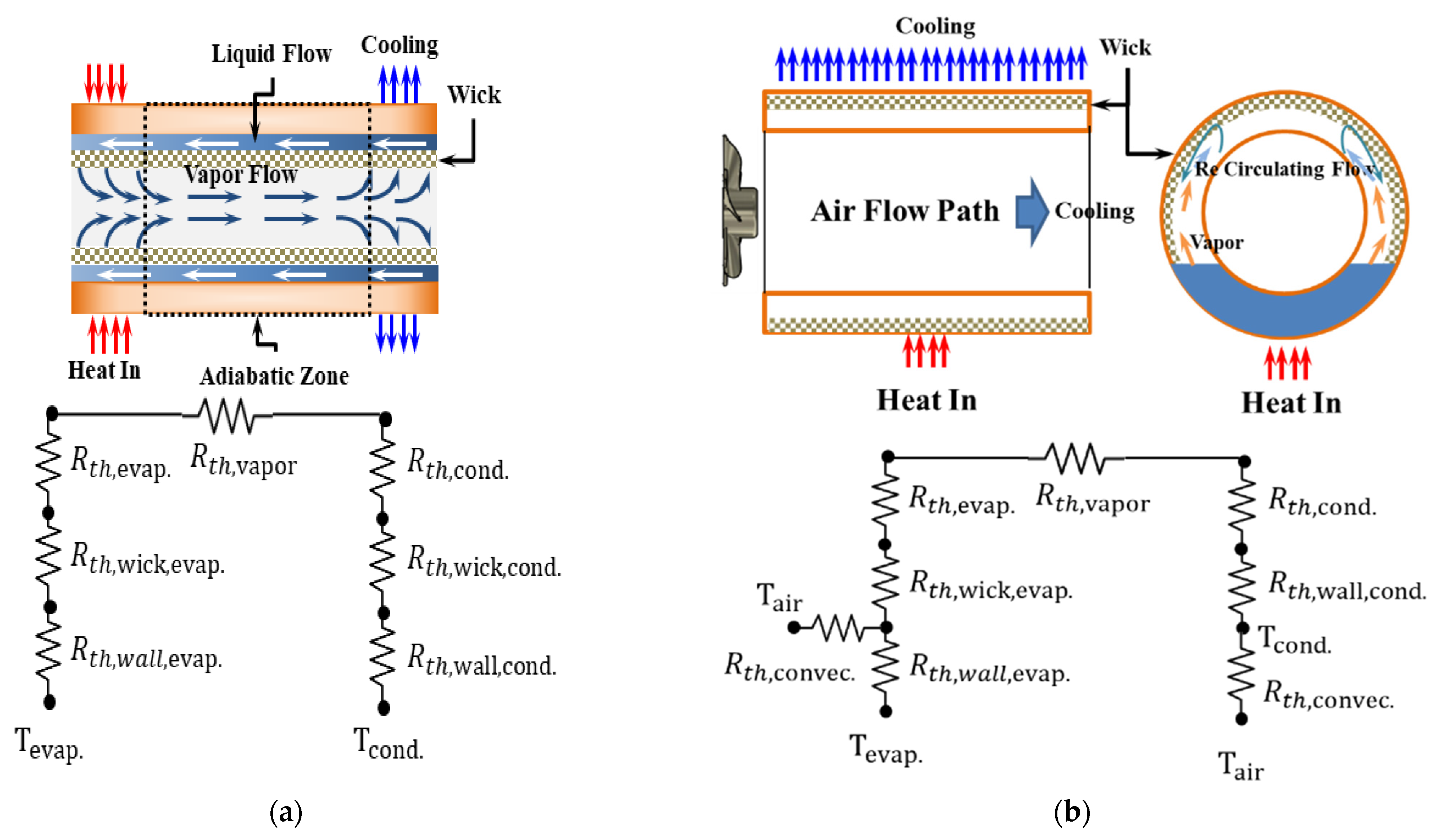
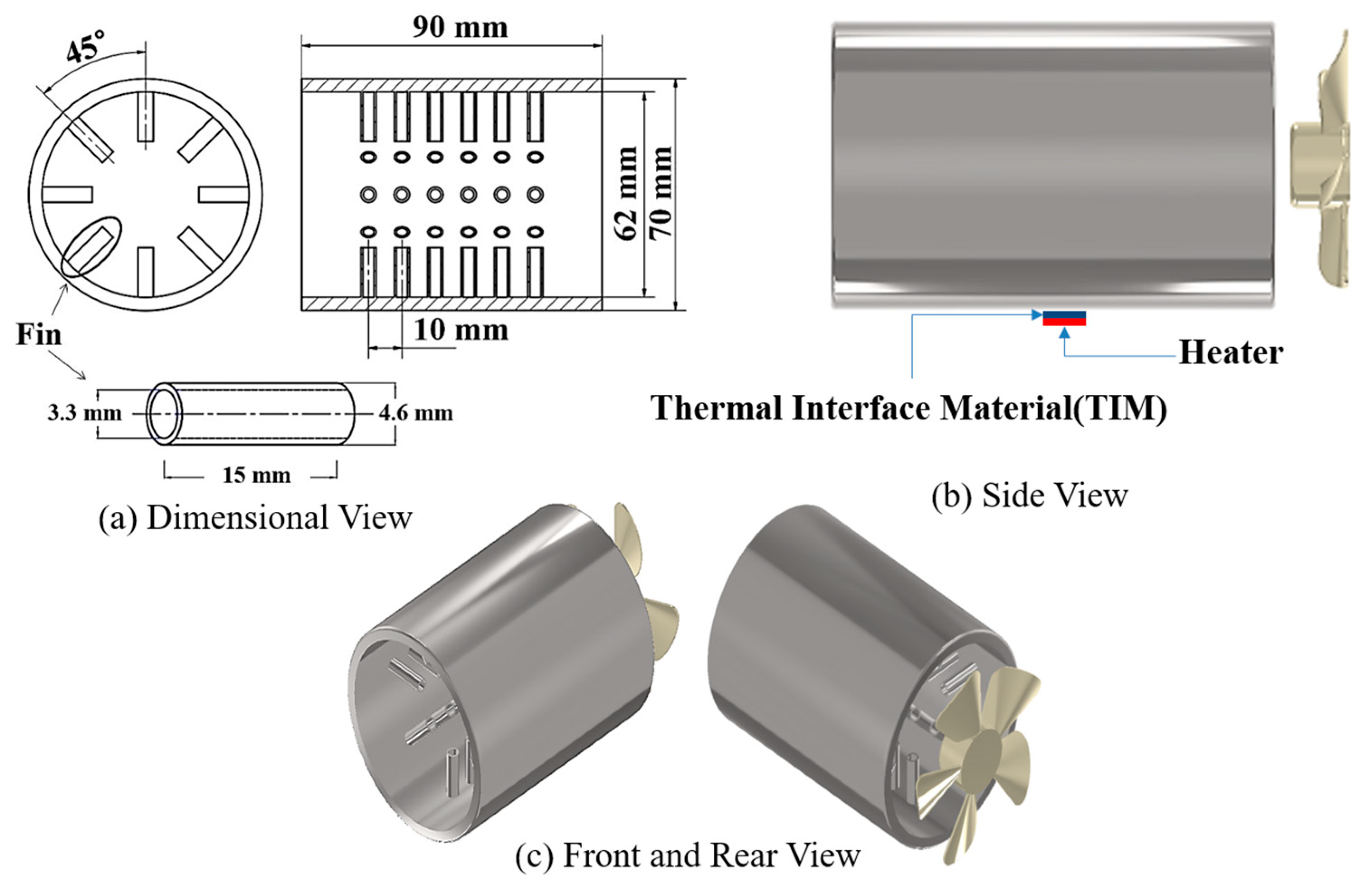
2. Concentric Annular Heat Pipe
3. The Numerical Analysis Method
- -
- The wick structure is completely immersed;
- -
- The flow in the wick is classified as Darcy’s flow;
- -
- If the flow in the wick is Darcy’s flow and completely immersed, effective thermal conductivity can be applied to the wick structure;
- -
- After condensation, the liquid film only occurs at the inner wall and wick;
- -
- The contact resistance of the fin is neglected, and the adiabatic condition is applied to the end of the fin.
3.1. Effective Thermal Conductivity Model
3.2. One-Dimensional Modeling of CAHP and Boundary Conditions
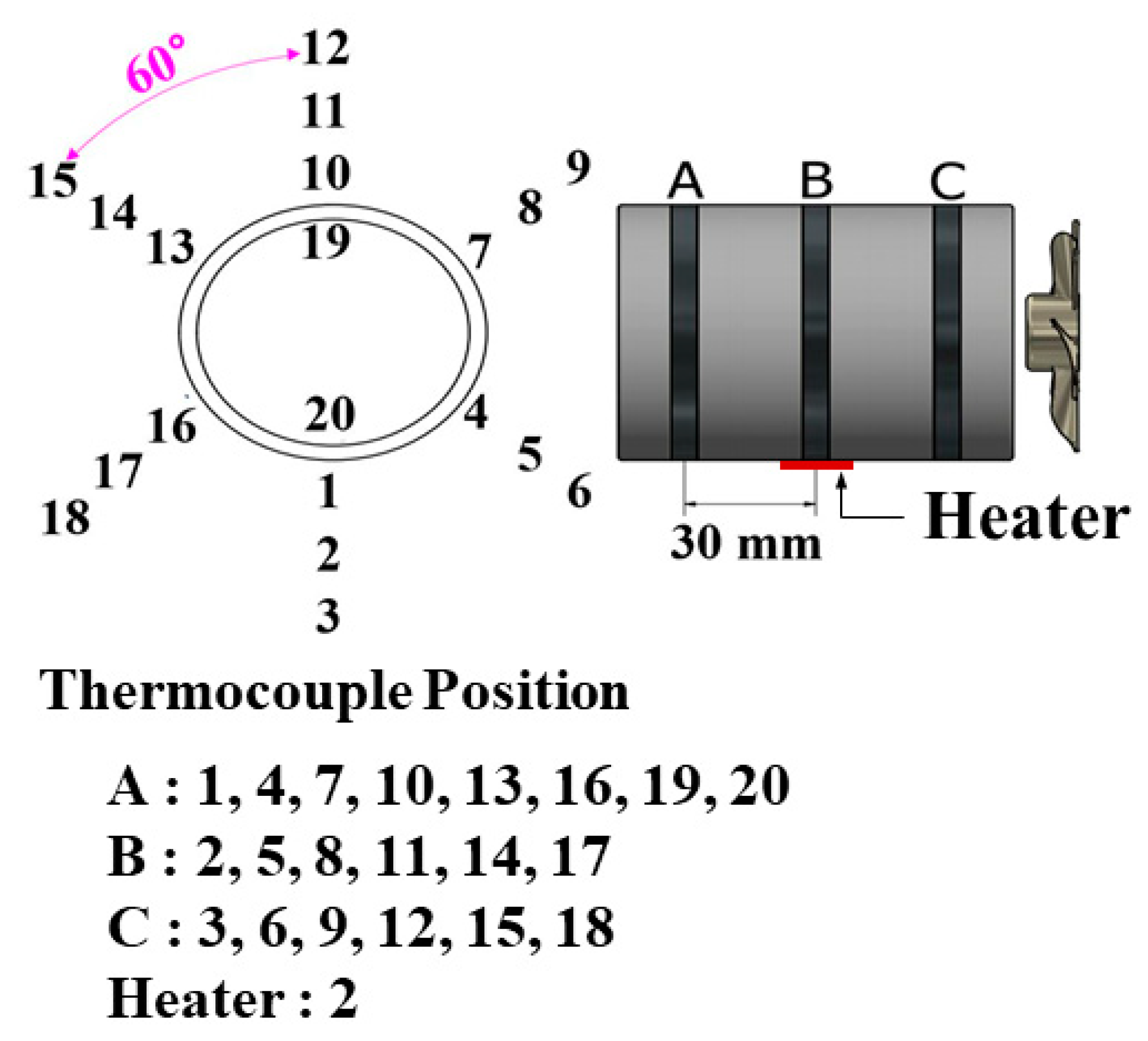
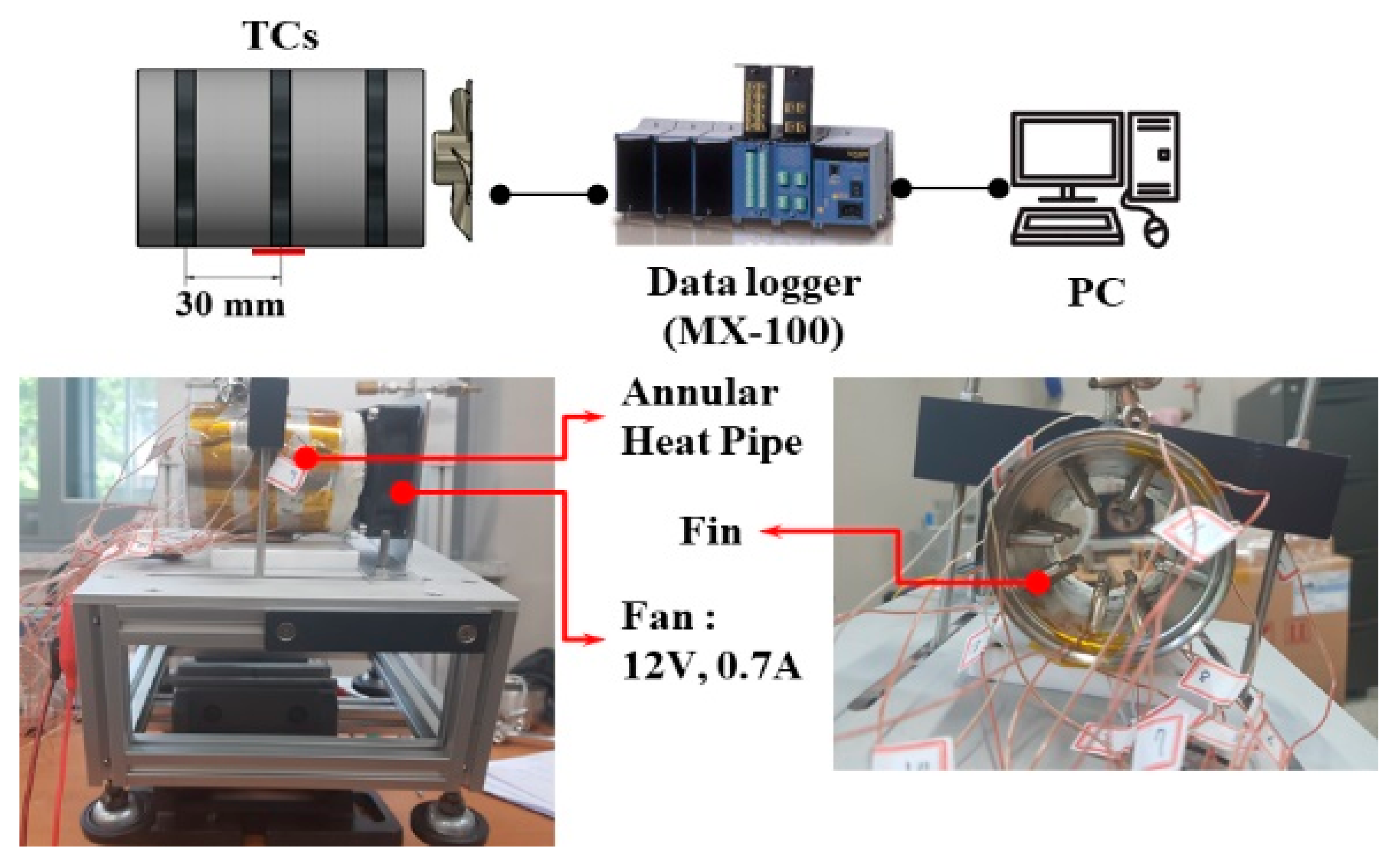
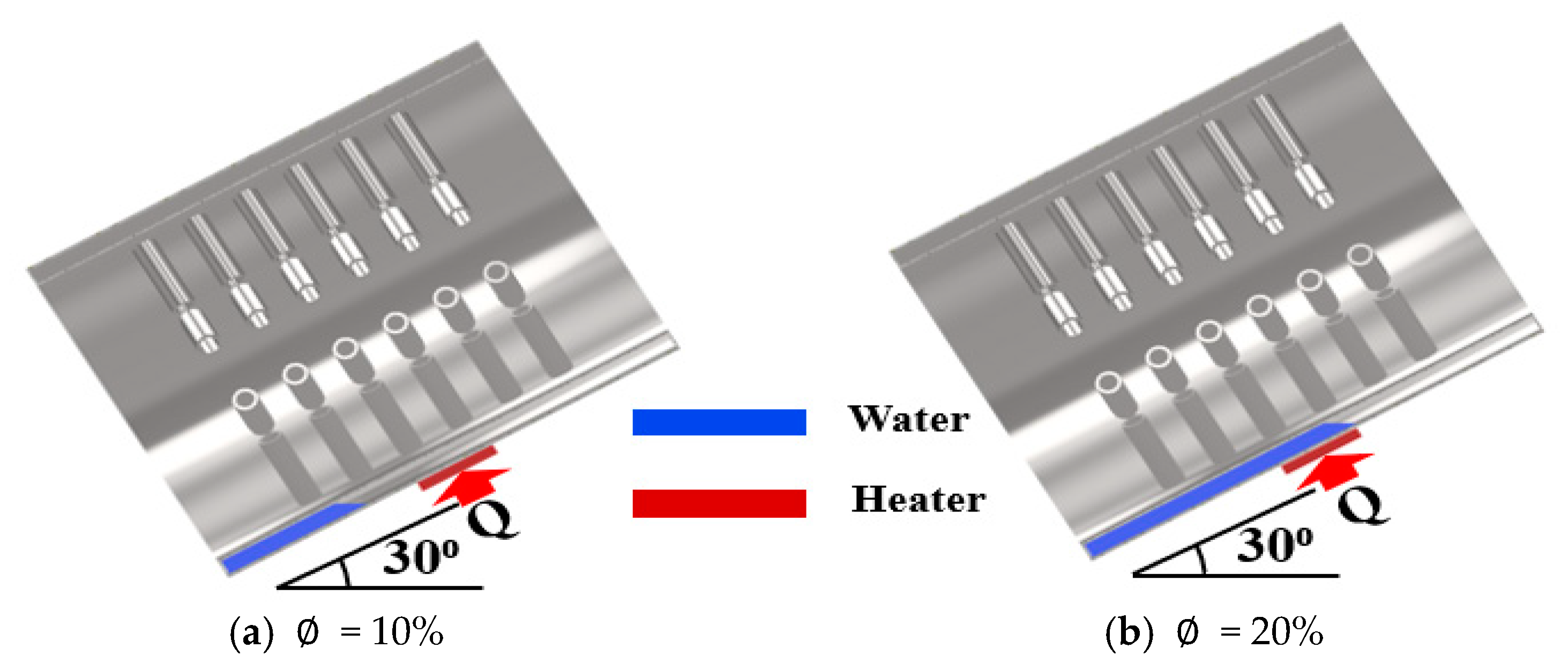
4. Experimental Equipment and Conditions
5. Results and Discussions
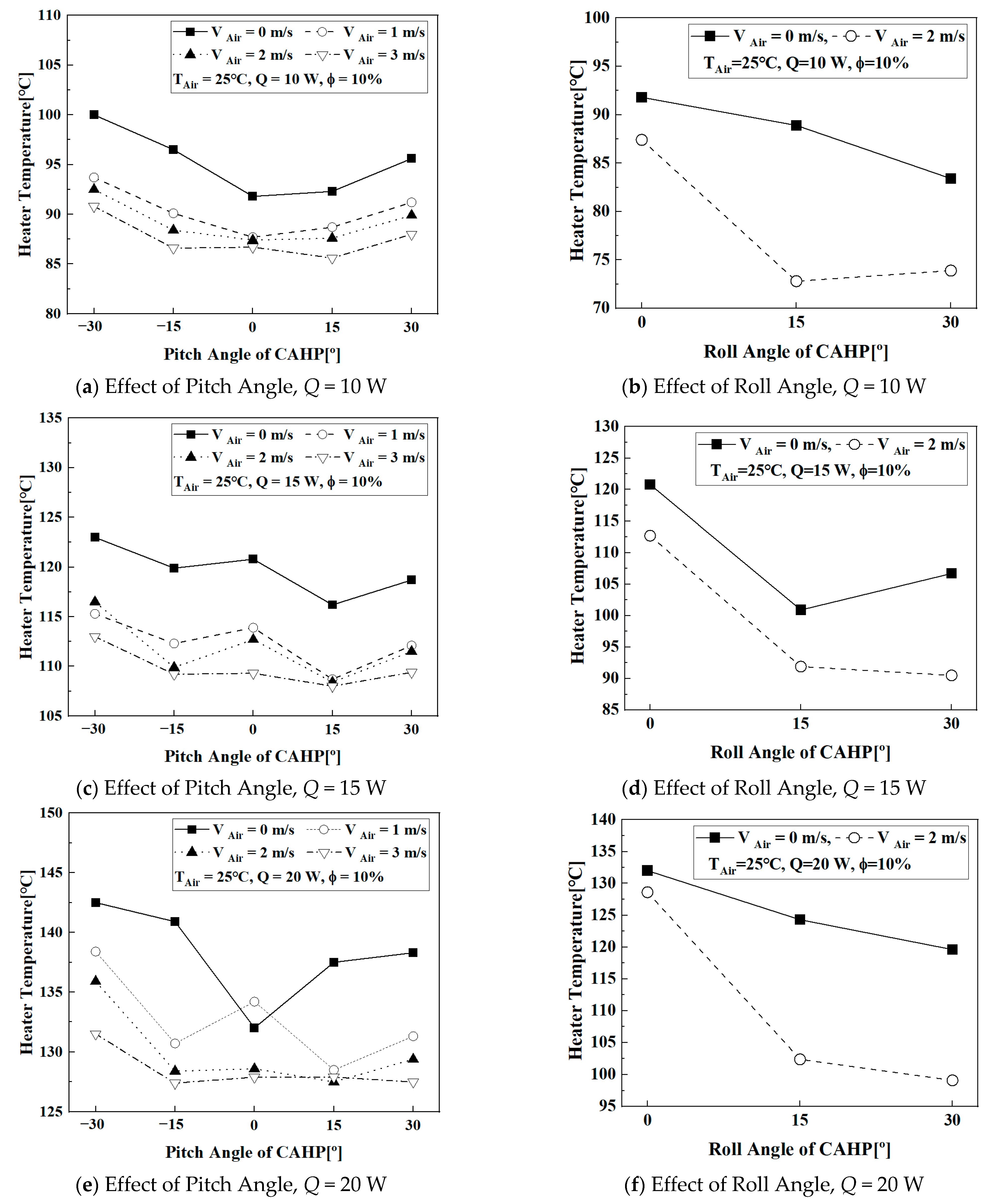
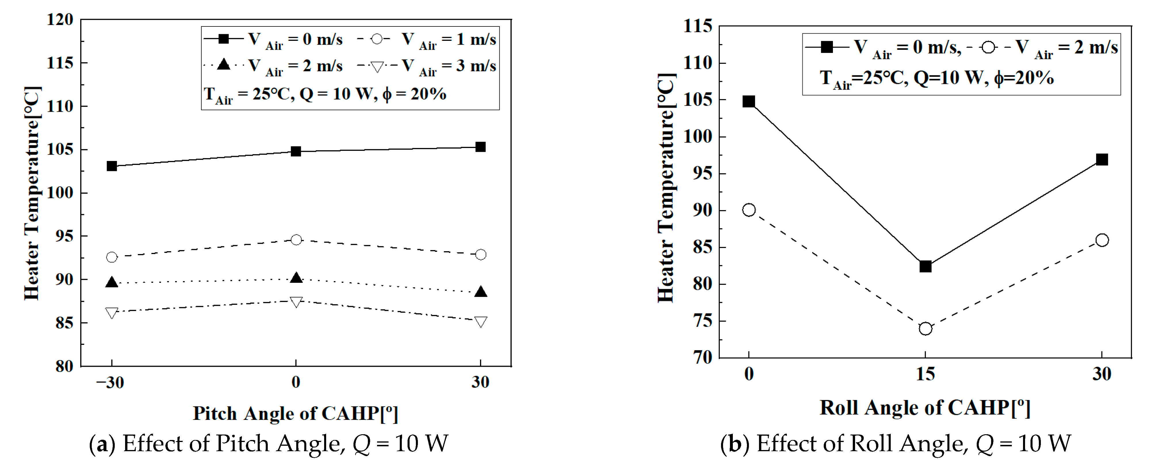
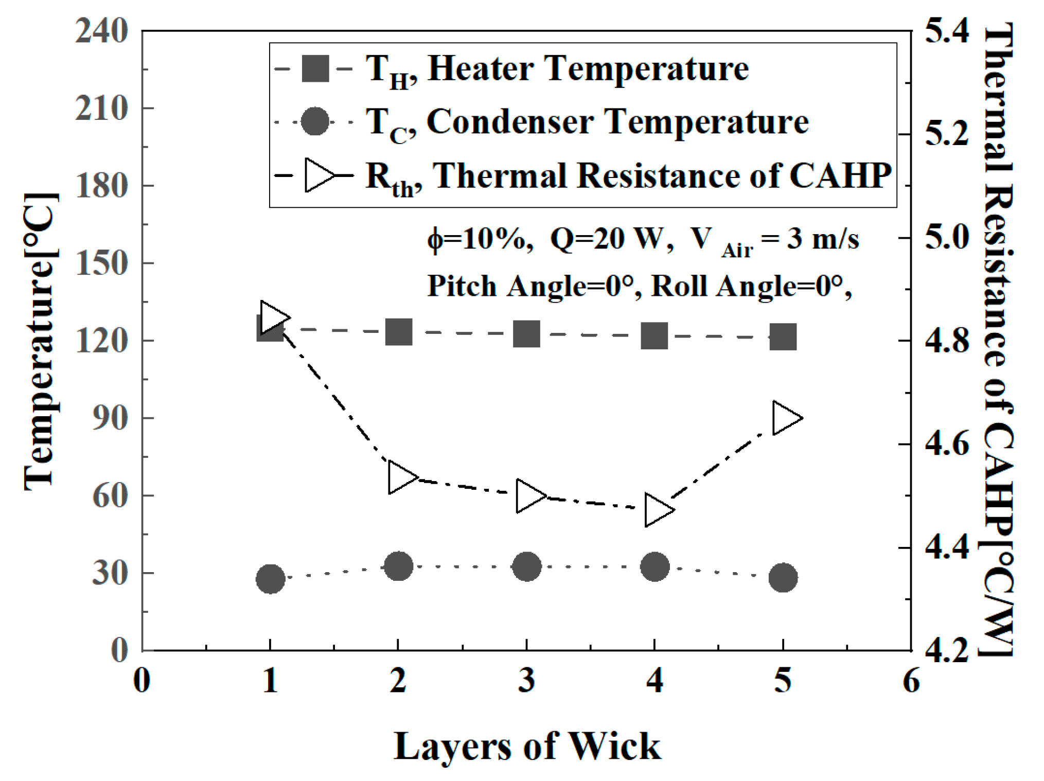
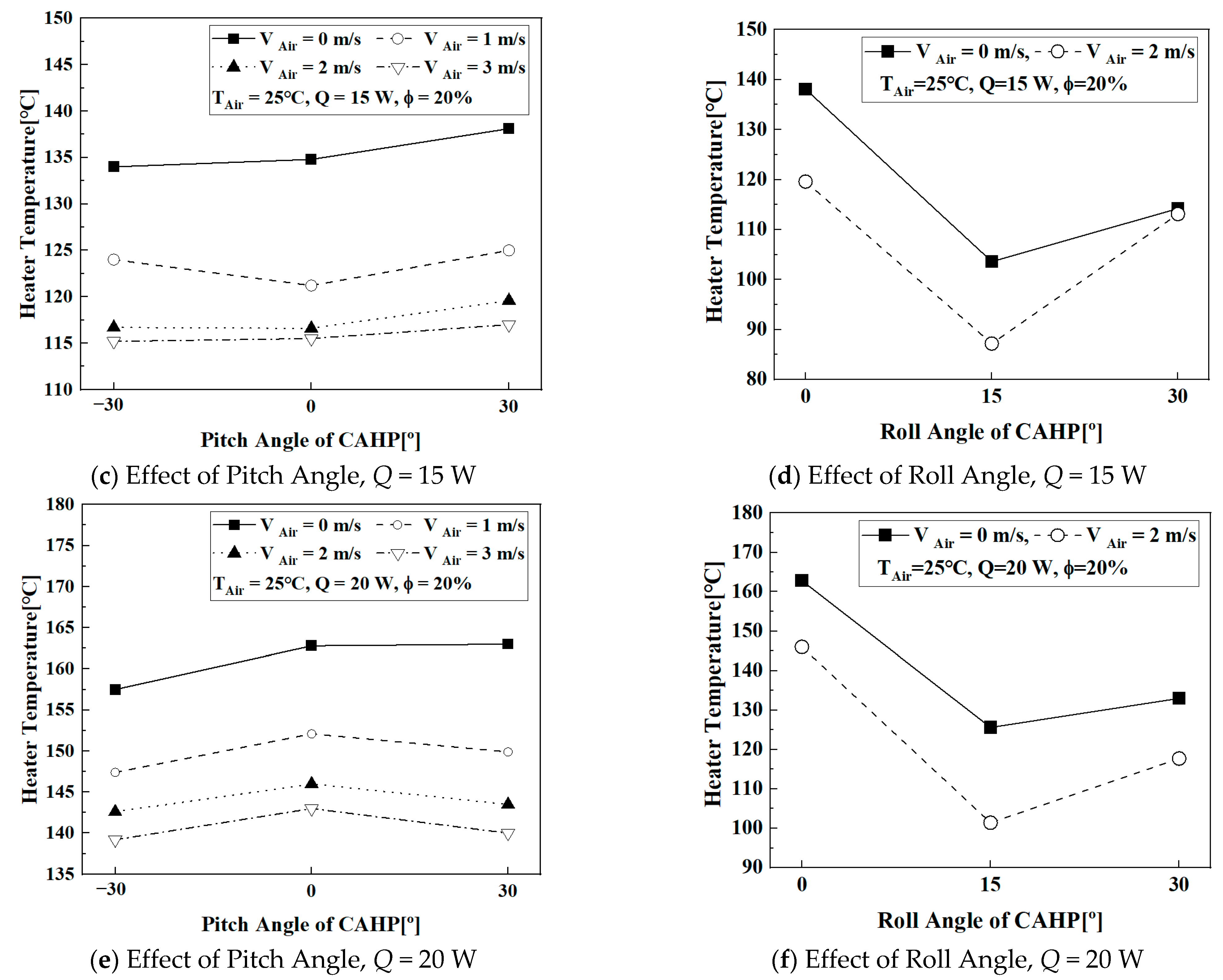
5.1. Experimental Results
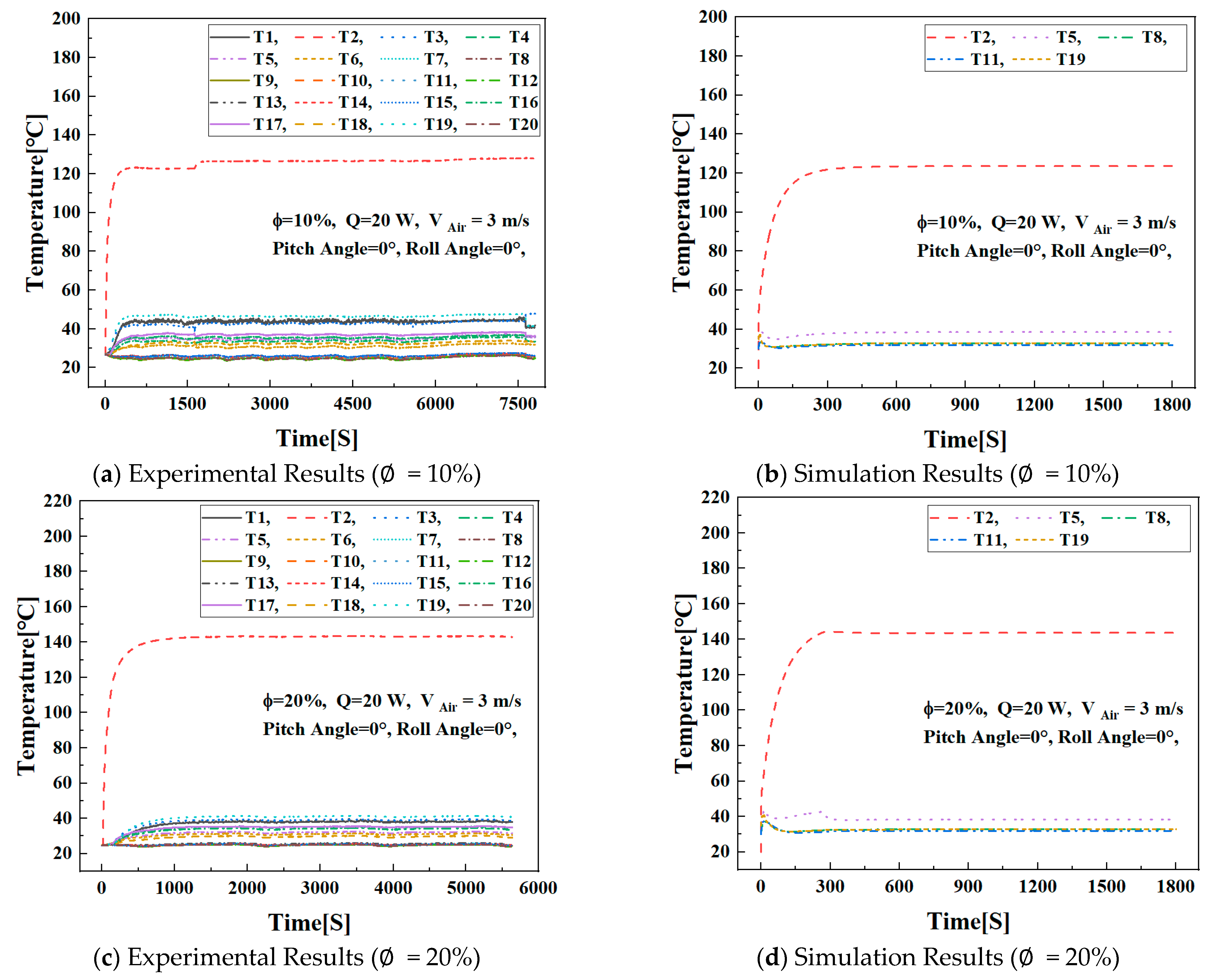
5.2. Comparison between the Experiment and Simulation on Transient Temperature Variation
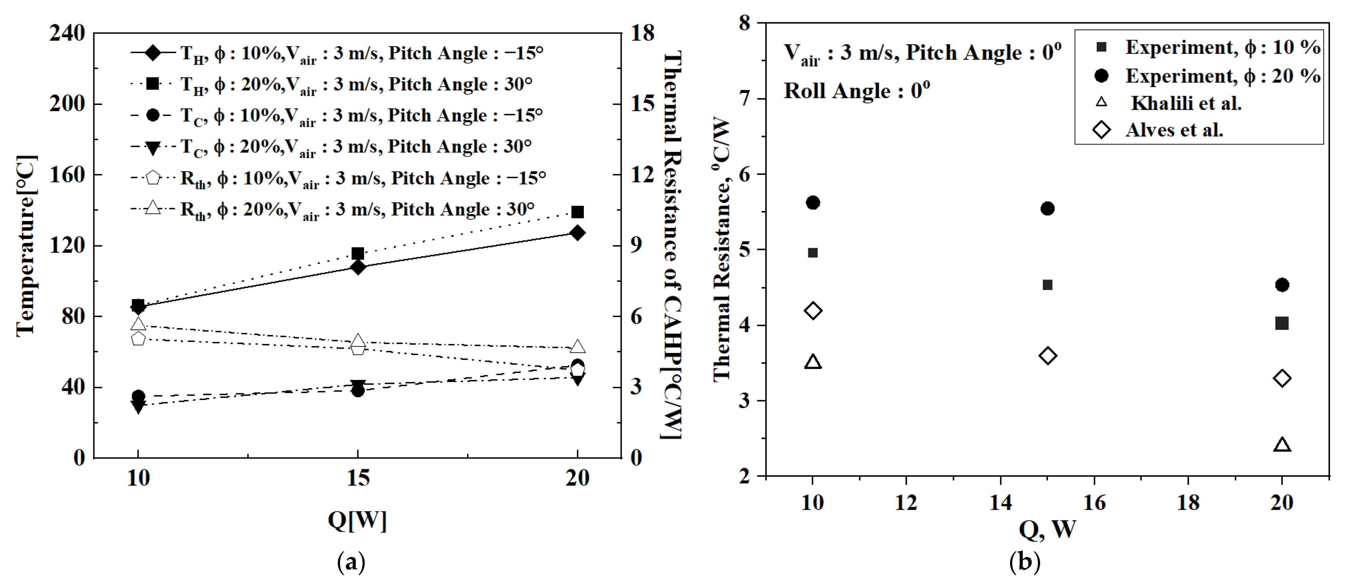
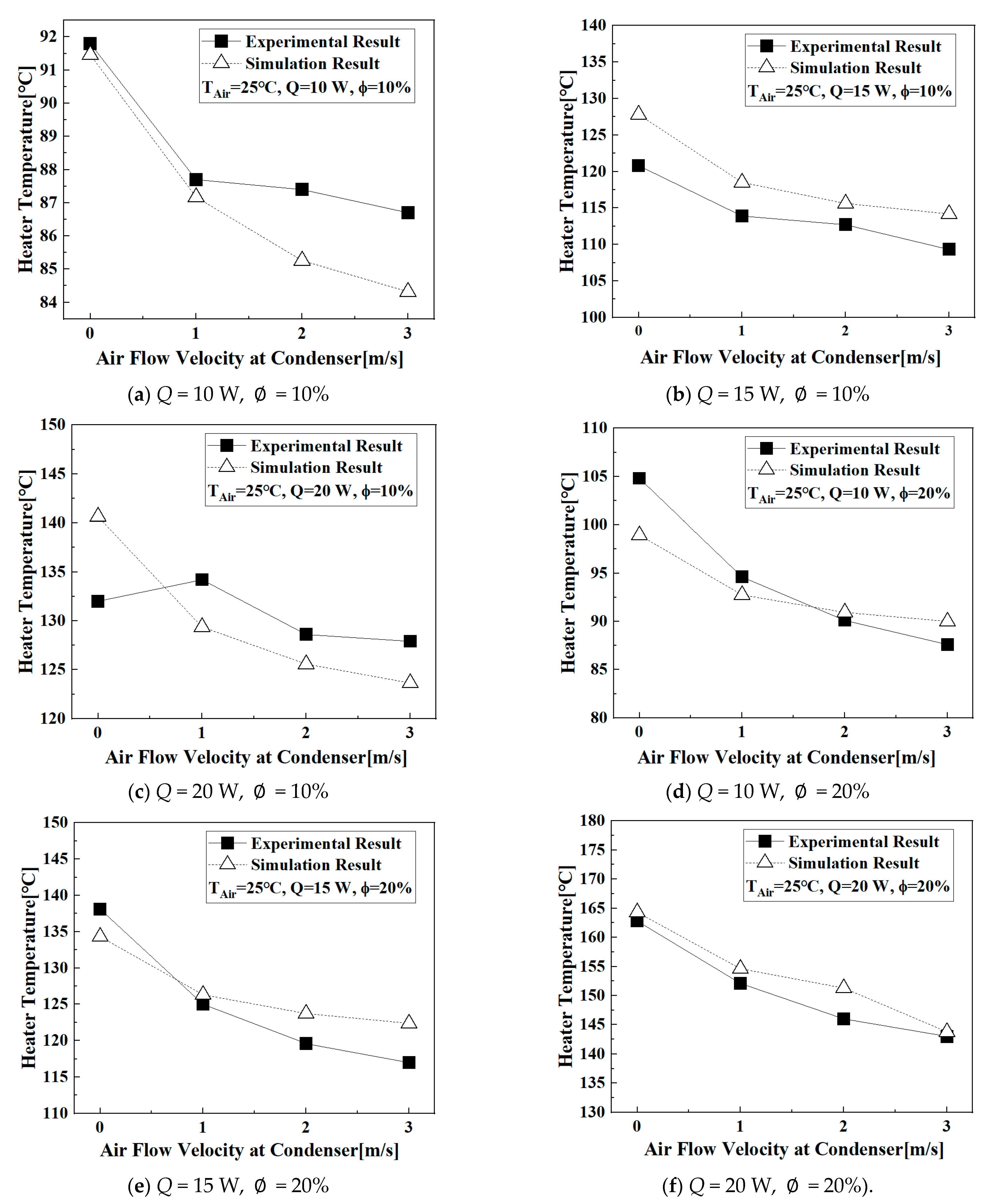
5.3. Comparison between the Experiment and Simulation on Thermal Performance
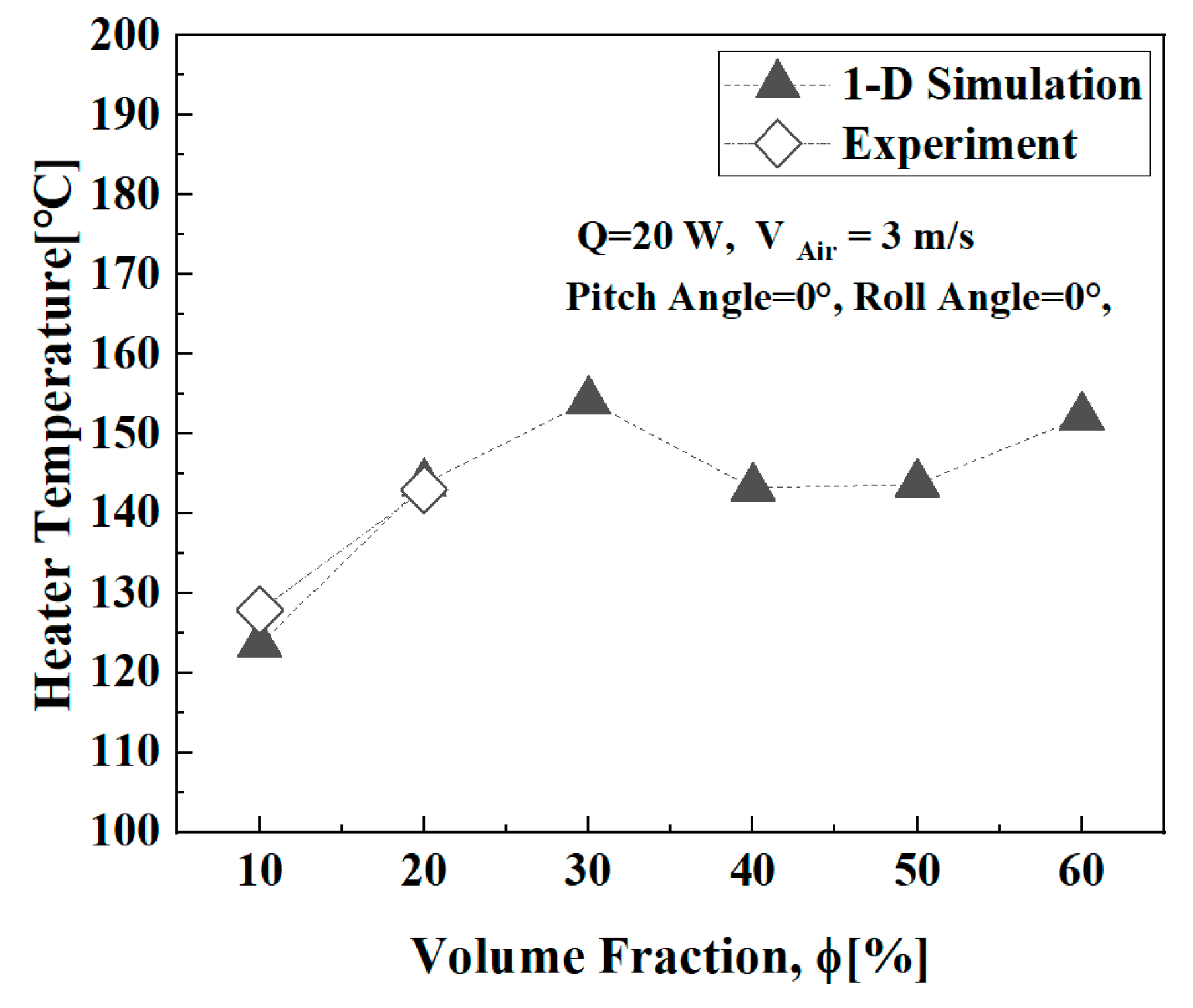
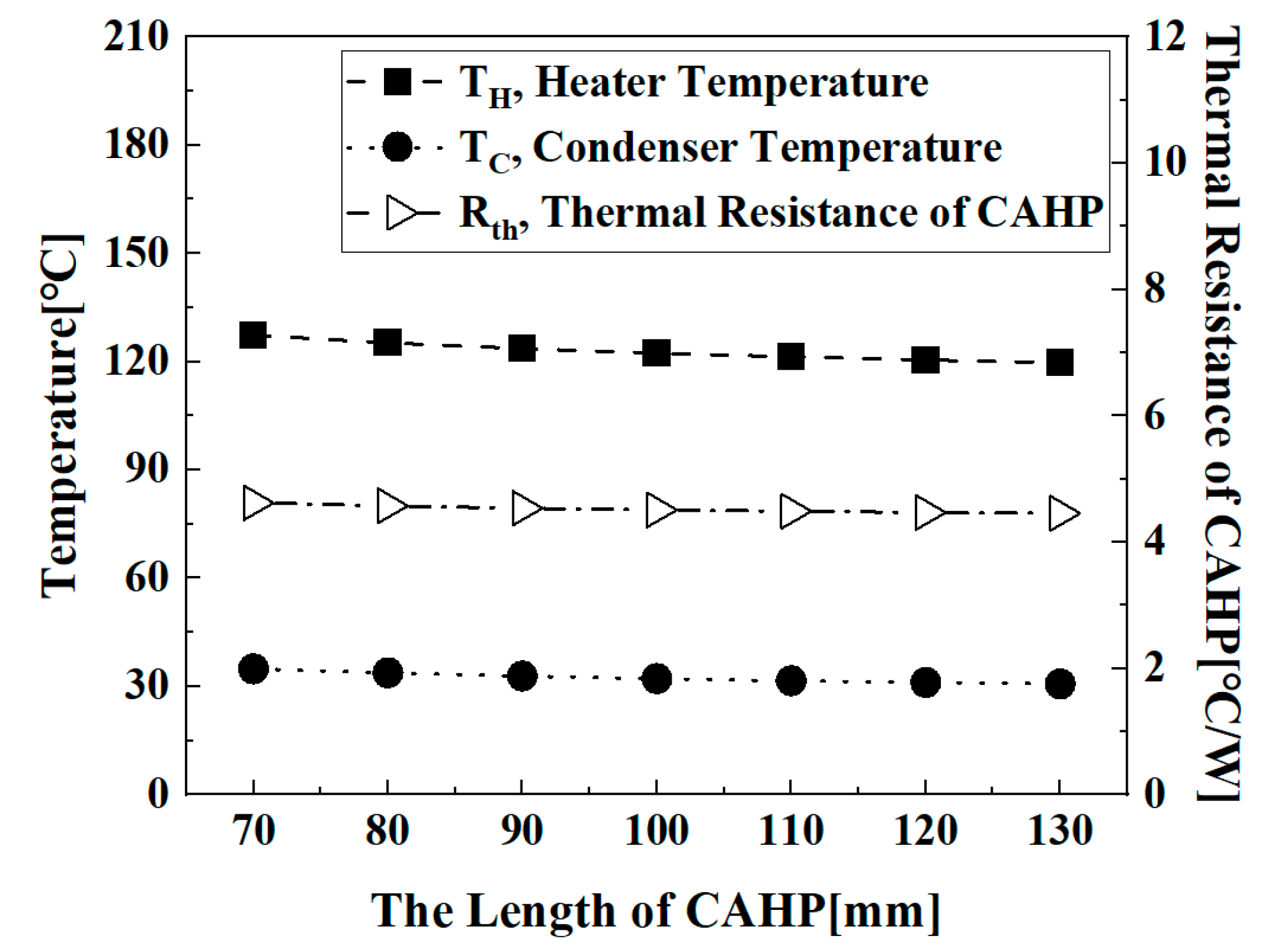
5.4. Investigation for Thermal Characteristics of CAHP Using One-Dimensional Analysis
6. Conclusions
Author Contributions
Funding
Institutional Review Board Statement
Informed Consent Statement
Data Availability Statement
Conflicts of Interest
Nomenclature
| Area, | |
| Specific heat capacity, | |
| F | Correction factor |
| f | Fiction coefficient |
| Grashof number (dimensionless) | |
| Specific enthalpy of vapor, | |
| Specific enthalpy of liquid, | |
| Convective heat transfer coefficient, | |
| Thermal conductivity, | |
| Length, | |
| Length of CAHP, | |
| Latent heat of fluid, | |
| M | Convection variables in fin efficiency equation in Equations (28) and (29) |
| Total mass of the working fluid, | |
| Mass flow rate, kg/s | |
| Nusselt number (dimensionless) | |
| Perimeter of fin, | |
| Static pressure, | |
| Prandtl number (dimensionless) | |
| Heat transfer rate, W | |
| Heat flux, W/m2 | |
| Thermal resistance, °C/W | |
| Rayleigh number (dimensionless) | |
| Reynolds number (dimensionless) | |
| Absolute Roughness, m | |
| Radius of internal outer surface of CAHP, | |
| Radius of internal inner surface of CAHP, | |
| Static temperature, °C | |
| t | thickness, m |
| Volume, | |
| w | Uncertainty of variables. |
| x | Quality |
| Greek | |
| Porosity, | |
| Fin efficiency | |
| Dynamic viscosity, | |
| Density, | |
| Volume fraction of charged working fluid, (VWorking Fluid/VTotal Volume) × 100 | |
| Subscripts | |
| Surrounding air | |
| 0 | Reference |
| a | Adiabatic |
| Air | Cooling air |
| base | Fin base |
| c | Condenser |
| cr | Critical |
| cv | Convective boiling |
| eff | Effective |
| f | Fin, or fluid |
| f,c | Fin cross sectional |
| g | Vapor, or denoted as v |
| l | Liquid |
| lf | Liquid film |
| LO | Liquid only |
| h | Hydraulic |
| HP | Heat pipe |
| NcB | Nucleate boiling |
| Q | Heat load |
| R | Resistance |
| s | Solid |
| surf | Surface |
| red | Reduced |
| TP | Two-Phase |
| VO | Vapor only |
| wick | Wick |
References
- He, Z.; Yan, Y.; Zhang, Z. Thermal management and temperature uniformity enhancement of electronic devices by micro heat sinks: A review. Energy 2021, 216, 119223. [Google Scholar] [CrossRef]
- IEA. World Energy Outlook; OECD; IEA: Paris, France, 2020. [Google Scholar]
- Zhang, X.; Kong, X.; Li, G.; Li, J. Thermodynamic assessment of active cooling/heating methods for lithium-ion batteries of electric vehicles in extreme conditions. Energy 2014, 64, 1092–1101. [Google Scholar] [CrossRef]
- Faghri, A. Heat Pipe Science and Technology; Taylor and Francis: Washington, DC, USA, 1995. [Google Scholar]
- Reay, D.A.; Kew, P.A.; McGlen, R.J. Heat Pipes Theory, Design and Applications, 6th ed.; Butterworth-Heinemann: Oxford, UK, 2014; pp. 207–225. [Google Scholar]
- Zhang, Z.; Wang, X.; Yan, Y. A review of the state-of-the-art in electronic cooling, e-Prime—Advances in Electrical Engineering. Electron. Energy 2021, 1, 100009. [Google Scholar] [CrossRef]
- Yu, T.-P.; Lee, Y.-L.; Li, Y.-W.; Mao, S.-W. The Study of Cooling Mechanism Design for High-Power Communication Module with Experimental Verification. Appl. Sci. 2021, 11, 5188. [Google Scholar] [CrossRef]
- Elnaggar, M.H.A.; Edwan, E. Heat Pipes for Computer Cooling Applications. In Electronics Cooling; Intech Open Science: London, UK, 2016; Chapter 4; pp. 52–73. [Google Scholar]
- Smakulski, P.; Pietrowicz, S. A review of the capabilities of high heat flux removal by porous materials, microchannels and spray cooling techniques. Appl. Therm. Eng. 2016, 104, 636–646. [Google Scholar] [CrossRef]
- Lee, J.H. Thermal Management Technology of TGP for High Heat-generation. Korean Soc. Mech. Eng. 2020, 12, 32–36. [Google Scholar]
- Faghri, A. Review and Advances in Heat Pipe Science and Technology. J. Heat Transf. 2012, 134, 123001. [Google Scholar] [CrossRef]
- Faghri, A.; Chen, M.; Morgan, M. Heat Transfer Characteristics in Two-Phase Closed Conventional and Concentric Annular Thermosyphons. ASME J. Heat Transf. 1989, 111, 611–618. [Google Scholar] [CrossRef]
- Faghri, A.; Thomas, S. Performance Characteristics of a Concentric Annular Heat Pipe: Part I—Experimental Prediction and Analysis of the Capillary Limit. J. Heat Transf. 1989, 111, 844–850. [Google Scholar] [CrossRef]
- Faghri, A.; Thomas, S. Performance Characteristics of a Concentric Annular Heat Pipe: Part II—Vapor Flow Analysis. J. Heat Transf. 1989, 111, 851–857. [Google Scholar] [CrossRef]
- Boo, J.H.; Park, S.Y. An Experimental Study on the Thermal Performance of a Concentric Annular Heat Pipe. J. Med. Sci. Technol. 2005, 19, 1036–1043. [Google Scholar] [CrossRef]
- Yan, X.K.; Duan, Y.N.; Ma, C.F.; Lv, Z.F. Construction of Sodium Heat-Pipe Furnaces and the Isothermal Characteristics of the Furnaces. Int. J. Thermophys. 2011, 32, 494–504. [Google Scholar] [CrossRef]
- Choi, J.H.; Yuan, Y.; Borca-Tasciuc, D.A.; Kang, H.K. Design, construction, and performance testing of an isothermal naphthalene heat pipe furnace. Rev. Sci. Instrum. 2014, 85, 095105. [Google Scholar] [CrossRef] [PubMed]
- Kammuang-lue, N.; Sakulchangsatjatai, P.; Terdtoon, P. Effect of Working Orientations, Mass Flow Rates, and Flow Directions on Thermal Performance of Annular Thermosyphon. In Proceedings of the 8th International Conference on Mechanical and Aerospace Engineering 2017, Prague, Czech Republic, 22–25 July 2017; pp. 171–178. [Google Scholar]
- Mustaffar, A.; Anh, N.P.; Reay, D.; Boodhooa, K. Concentric annular heat pipe characterization analysis for a drying application. Appl. Therm. Eng. 2019, 149, 275–286. [Google Scholar] [CrossRef]
- Song, E.-H.; Lee, K.-B.; Rhi, S.-H.; Kim, K. Thermal and Flow Characteristics in a Concentric Annular Heat Pipe Heat Sink. Energies 2020, 13, 5282. [Google Scholar] [CrossRef]
- Song, E.-H.; Lee, K.-B.; Rhi, S.-H. Thermal and Flow Simulation of Concentric Annular Heat Pipe with Symmetric or Asymmetric Condenser. Energies 2021, 14, 3333. [Google Scholar] [CrossRef]
- Czajkowski, C.; Nowak, A.I.; Pietrowicz, S. Flower Shape Oscillating Heat Pipe—A novel type of oscillating heat pipe in a rotary system of coordinates—An experimental investigation. Appl. Therm. Eng. 2020, 179, 115702. [Google Scholar] [CrossRef]
- Błasiak, P.; Opalski, M.; Parmar, P.; Czajkowski, C.; Pietrowicz, S. The Thermal—Flow Processes and Flow Pattern in a Pulsating Heat Pipe—Numerical Modelling and Experimental Validation. Energies 2021, 14, 5952. [Google Scholar] [CrossRef]
- Khalili, M.; Shafii, M. Investigating thermal performance of a partly sintered-wick heat pipe filled with different working fluids. Sci. Iran. 2016, 23, 2616–2625. [Google Scholar] [CrossRef] [Green Version]
- Alves, T.A.; Krambeck, L.; Santos, P.H.D. Heat Pipe and Thermosyphon for Thermal Management of Thermoelectric Cooling. In Bringing Thermoelectricity into Reality, 1st ed.; Aranguren, P., Ed.; Intech Open: London, UK, 2018; Chapter 17. [Google Scholar]
- Kapekov, A. Development of an Innovative Cooling Concept for Turbofan Engines; KTH School of Industrial Engineering and Management: Stockholm, Sweden, 2018. [Google Scholar]
- Liu, F.; Lan, F.; Chen, J. Dynamic thermal characteristics of heat pipe via segmented thermal resistance model for electric vehicle battery cooling. J. Power Sources 2016, 321, 57–70. [Google Scholar] [CrossRef]
- Lee, Y.Y. An Investigation and Enhancement of Thermal Performance in a Heat Pipe and Its Thermal Modeling Application. Ph.D. Dissertation, Swinburne University of Technology, Kuching, Malaysia, 2018. [Google Scholar]
- Shafieian, A.; Khiadani, M.; Nosrati, A. Theoretical modeling approaches of heat pipe solar collectors in solar systems: A comprehensive review. Sol. Energy 2019, 193, 227–243. [Google Scholar] [CrossRef]
- Ciacci, C. 1D Modelling and Analysis of Thermal Conditioning Systems for Electric Vehicles. Ph.D. Dissertation, University of Windsor, Windsor, ON, Canada, 2019. Available online: https://scholar.uwindsor.ca/etd/7779 (accessed on 19 January 2022).
- Hu, G.; Hu, R.; Kelly, J.M.; Ortensi, J. Multi-Physics Simulations of Heat Pipe Micro Reactor; Report ID ANL-NSE-19/25; Argonne National Laboratory: Lemont, IL, USA, 2019. [Google Scholar]
- Yoo, J.; Qin, S.; Song, M.; Hartvigsen, J.L.; Sellers, Z.D.; Morton, T.J.; Sabharwall, P.; Hansel, J.; Ibarra, L.; Feng, B.; et al. Modeling and Analysis Support for High Temperature Single Heat Pipe Experiment: Current Status and Plan; Report# INL/EXT-21-61961; Idaho National Laboratory: Idaho Falls, ID, USA, 2021. [Google Scholar]
- Dong, Z.; Li, X.; Li, Z.; Hou, Y. Modeling Simulation and Temperature Control on Thermal Characteristics of Airborne Liquid Cooling System. IEEE Access 2020, 8, 113112–113120. [Google Scholar] [CrossRef]
- Tao, X. Design, Modeling and Control of a Thermal Management System for Hybrid Electric Vehicles. Ph.D. Dissertation, Clemson University, Clemson, SC, USA, 2016. [Google Scholar]
- Ayad, M.; Jubori, A.; Jawad, Q.A. Computational evaluation of thermal behavior of a wickless heat pipe under various conditions. Case Stud. Therm. Eng. 2020, 22, 100767. [Google Scholar] [CrossRef]
- Adrian, Ł.; Szufa, S.; Piersa, P.; Mikołajczyk, F. Numerical Model of Heat Pipes as an Optimization Method of Heat Exchangers. Energies 2021, 14, 7647. [Google Scholar] [CrossRef]
- Zhao, Z.; Zhang, Y.; Zhang, Y.; Zhou, Y.; Hu, H. Numerical Study on the Transient Thermal Performance of a Two-Phase Closed Thermosyphon. Energies 2018, 11, 1433. [Google Scholar] [CrossRef] [Green Version]
- Girish, S.; Lavanya, K.; Krishna, P.G. CFD analysis of Pulsating heat pipe using different fluids. Int. J. Mech. Eng. Technol. (IJMET) 2017, 8, 804–812. [Google Scholar]
- Kloczko, S. Experimental Investigation and Numerical Simulation of Loop Thermosyphons. Master’s Thesis, University of Connecticut, Mansfield, CT, USA, 2019. [Google Scholar]
- Rhi, S.H.; Lee, K.B.; Chae, H.I. 3-Dimensional Annular Heat Sink. Korea Patent No. 10-2019-0133835, 25 October 2019. [Google Scholar]
- SIEMENS. Integration Algorithms and Library User Guides Used in Simcenter Amesim; SIEMENS: Munich, Germany, 2020. [Google Scholar]
- Brennan, P.J.; Kroliczek, E.J. Heat Pipe Design Handbook; National Aeronautics and Space Administration: Washington, DA, USA, 1979. [Google Scholar]
- Holman, J.P. Heat Transfer, 10th ed.; McGraw-Hill Book Company: New York, NY, USA, 2010. [Google Scholar]
- Park, Y.Y.; Jeong, Y.S.; Bang, I.C. Design Study of Heat Pipes for Nuclear Spaceship Applications. In Proceedings of the Transactions of the Koran Nuclear Society Spring Meeting, Jeju, Korea, 23–24 May 2019. [Google Scholar]
- National Instruments. Calculating Thermocouple Measurement Error in DMM/Switch Temperature Measurement Systems. In Tutorial of National Instruments; National Instruments: Austin, TX, USA, 2012. [Google Scholar]


| Material | Density [kg/m3] | Thermal Conductivity [W/m2K] | Specific Heat [J/kg-K] |
|---|---|---|---|
| Stainless steel 304 | 8000 | 16.3 | 530 |
| Thermal Interface Material (TIM) | 250 | 0.73 | 0.87 |
| Heater (Si3N4) | 3200 | 20 | 660 |
| Variables | Values |
|---|---|
| Wick (500 mesh, Stainless steel 304) | 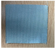 |
| 16.3 | |
| 0.659 | |
| 0.345 | |
| 13.74 | |
| [kg/m3] | 8000 |
| [kg/m3] | 980.49 |
| [kg/m3] | 5576 |
| [J/kg-K] | 530 |
| [J/kg-K] | 4138 |
| [J/kg-K] | 1791 |
| Volume Fraction [%] | Total Mass of Working Fluid [kg] | Thickness of Liquid Film [mm] |
|---|---|---|
| 10 | 0.09 | |
| 20 | 0.43 | |
| 30 | 0.018 | 0.77 |
| 40 | 0.024 | 1.11 |
| 50 | 0.030 | 1.44 |
| 60 | 0.036 | 1.76 |
| 70 | 0.042 | 2.09 |
| 80 | 0.048 | 2.41 |
| Library Component | Component Name | Description | Library Component | Component Name | Description |
|---|---|---|---|---|---|
 | Transformer | thermodynamic state transformer |  | Thermal node | thermal temperature (fixed by port 4) and heat flow node |
 | Fluid properties | refrigerant thermodynamic properties with working fluids |  | Heat source | conversion of signal to a heat flow |
 | Modulated source | modulated mass and enthalpy flow rate source |  | External mixed convection | external mixed convective exchange with various convection models |
 | Fluid property sensor | generic sensor with additional thermodynamic state variable |  | Convective exchange | generic conduction |
 | Two-phase flow pipe volume | pipe with heat exchange with 2 thermal ports (C-R), related to various two-phase flow models |  | Thermal capacitance | thermal capacity |
 | Solid properties | thermal solid properties with various materials |  | Mathematical function | signal function of inputs x and y |
 | Power sensor | power/energy/activity sensor with offset and gain |  | Sign inverter | reverses the sign of the input |
 | Gain | outputs a signal with a constant specified value |  | Generic sensor | calculates additional thermodynamic state variables |
| Variables | Values |
|---|---|
| Q: Heat In [W] | 10, 15, 20 |
| 10, 20 | |
| Vair: Air Flow Rate [m/s] | 0, 1, 2, 3 |
| Pitch Angle [°] | −30, −15, 0, 15, 30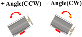 |
| Roll Angle [°] | 0, 15, 30 |
| Definition of Concentric Annular Heat Pipe Orientation | 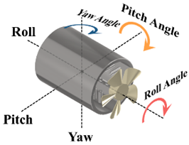 |
Publisher’s Note: MDPI stays neutral with regard to jurisdictional claims in published maps and institutional affiliations. |
© 2022 by the authors. Licensee MDPI, Basel, Switzerland. This article is an open access article distributed under the terms and conditions of the Creative Commons Attribution (CC BY) license (https://creativecommons.org/licenses/by/4.0/).
Share and Cite
Lee, J.-S.; Ahn, J.-H.; Chae, H.-I.; Lee, H.-C.; Rhi, S.-H. 1-D Modeling of Two Phase Flow Process in Concentric Annular Heat Pipe and Experimental Investigation. Processes 2022, 10, 493. https://doi.org/10.3390/pr10030493
Lee J-S, Ahn J-H, Chae H-I, Lee H-C, Rhi S-H. 1-D Modeling of Two Phase Flow Process in Concentric Annular Heat Pipe and Experimental Investigation. Processes. 2022; 10(3):493. https://doi.org/10.3390/pr10030493
Chicago/Turabian StyleLee, Ji-Su, Jae-Hyun Ahn, Heui-Il Chae, Hi-Chan Lee, and Seok-Ho Rhi. 2022. "1-D Modeling of Two Phase Flow Process in Concentric Annular Heat Pipe and Experimental Investigation" Processes 10, no. 3: 493. https://doi.org/10.3390/pr10030493
APA StyleLee, J.-S., Ahn, J.-H., Chae, H.-I., Lee, H.-C., & Rhi, S.-H. (2022). 1-D Modeling of Two Phase Flow Process in Concentric Annular Heat Pipe and Experimental Investigation. Processes, 10(3), 493. https://doi.org/10.3390/pr10030493