Comparative Study between Flatness-Based and Field-Oriented Control Methods of a Grid-Connected Wind Energy Conversion System

Abstract

Wind energy is an alternative to meet the growing energy demand. Control of wind turbines should help the reliability and stable operation of the power grid. Furthermore, they should respect the technical requirements according to the grid codes to inject the wind energy into the grid. In this paper, a well-known field-oriented control (FOC) method and a new control method based on the flatness properties (FBC) are presented and compared. These control methods are applied to a wind energy conversion system (WECS), which connects a variable-speed wind turbine (WT) based on a permanent magnet synchronous generator (PMSG) to the grid via a back-to-back converter. The main aim of both control methods is to extract the maximum power from the wind. For this purpose, the mathematical model of each subsystem, i.e., WT, PMSG, and electrical grid, is presented. To evaluate and to compare the dynamic behavior of the high-power wind energy conversion system, it is modeled and the control strategies are developed using SimPowerSystems Toolbox in MATLAB. The simulation results obtained in the time domain show that the FBC performs better at managing the energy in the studied system. Indeed, the proposed FBC is a high bandwidth control method with only one closed-loop control, which leads to a high dynamic performance. Therefore, that strategy can be used to provide ancillary services such as frequency control and spinning reserves according to the grid codes.

1. Introduction

Wind energy is an alternative to meet the growing energy demand and to protect the environment [1]. The Global Wind Energy Council has reported a global capacity of 651 GW with 60.4 GW of new installations in 2019 and an expectation of growth of more than 100 GW in annual installations over the next decade [2,3]. Research on the wind power industry started to improve in the last century where the variable-speed wind turbine (WT) with a full-scale frequency converter was used in distributed power generation systems [4,5,6,7,8]. The variable-speed WTs, the most common type of wind energy conversion systems (WECSs), are able to extract more power than the fixed-speed WTs can [9]. In this system, the utilization of PMSGs has more advantages in comparison with induction generators such as high efficiency and reliability. Therefore, PMSGs have become a more attractive solution for use in variable-speed wind turbine applications [10,11]. Indeed, the WT with the PMSG is an efficient configuration for variable-speed WTs. Some advantages of this configuration are dc excitation elimination, less maintenance cost, and high power-to-weight ratio. To connect the WT to the network, a full-scale converter is employed, which provides a wide operation range and more produced power [9].

Control strategies have influences on the dynamic stability of WTs [12]. Control of the wind generators is widely carried out with the field-oriented control (FOC) method [5,9,10]. It is the most used method of PMSG control. The main idea is the use of a coordinate system aligned to the rotor flux vector. That leads to a decoupled control of the rotor flux and the machine torque or speed. The transformed system variables are controlled with PI controllers. The control structure commonly consists of inner current control loops and outer speed/torque and flux control loops [5,13]. Due to the inherent nonlinearity of the machine model, control design requires different time constants for the inner and outer loops. In this method, the speed and position of the rotor should be known [13,14]. Some papers have been published to improve the performance and efficiency of this method. In order to minimize power losses in the generator and power converter, the authors of [15] proposed that the generator reactive current component be calculated and imposed on the generator. To improve the efficiency and the reliability of the control, a nonlinear sliding mode control strategy was applied to the wind power generation system under symmetrical and an asymmetrical grid voltage sags in [16,17], respectively. This method was also used to control a doubly fed induction generator-based WT [18]. Authors of [19] presented an output power smoothing method by a simple coordinated control of the DC-link voltage and the pitch angle of the PMSG-based WECS. The power smoothing was similarly realized in [20] by two control strategies that utilize the self-capability of the PMSG. Indeed, these methods are suitable for ensuring system operation security and reliability for islanded systems that have limited power reserves. A control strategy based on the average wind speed and standard deviation of wind speed and pitch angle control was developed, in which a generalized predictive control in all operating regions of a WT was employed. This approach was also used in [6] to reduce the power losses of an offshore wind farm. To improve the regulation performance of variable-speed WTs, a coordinated active power control strategy (PAC) was studied in [21]. It includes the simultaneous activation of the PAC and the rotor speed control. To attenuate the steep and large volatile dynamics during turbine switching between low and high wind speed mode, a modified algorithm was proposed in [22]. This algorithm modifies the generator torque control law in the low wind speed mode to reduce the steep change of turbine power and torque. However, to improve the behavior and dynamics of the system, a flatness-based control (FBC) was developed in this paper with just one control algorithm in all wind speeds. The developed FBC method was used to manage the energy in the WECS shown in Figure 1 and was compared with the FOC method. The main advantage of the FBC method is the ability of predicting behavior of the system in the transient state, as well as the steady state [23,24]. In [25], it was shown that this type of control can improve the performance of a three-phase PWM rectifier in the transient state in comparison with the traditional vector control method. It should be mentioned that increasing the wind energy penetration levels in modern power systems has led to a variety of technical, economic, and regulatory issues, involving the interaction between large wind farms and power systems. Many grid code versions of the transmission system operators express that wind farms must provide ancillary services such as frequency control and spinning reserves as with conventional power stations [26]. Furthermore, wind systems should enhance the capability of low-voltage ride-through (LVRT) [27]. A high dynamics control method such as FBC can be more effective at meeting these issues.

To control the system, it was shown that the system is flat at first, and then the appropriate trajectories should be generated and be planned on the components of the output variable vector of the system. Based on the research in the field of modern control, the FBC is expected to offer some advantages such as rejection of perturbations and robustness in comparison with the other methods [24]. In the next section, the overall structure of the model is presented. The FOC method is explained in Section 3 and the FBC method is presented in Section 4, where the system is divided by two subsystems and the proper outputs are chosen for each subsystem. The time domain simulation results for a 5 MW WT obtained in MATLAB-SimPowerSystems are presented, compared, and analyzed in Section 5.

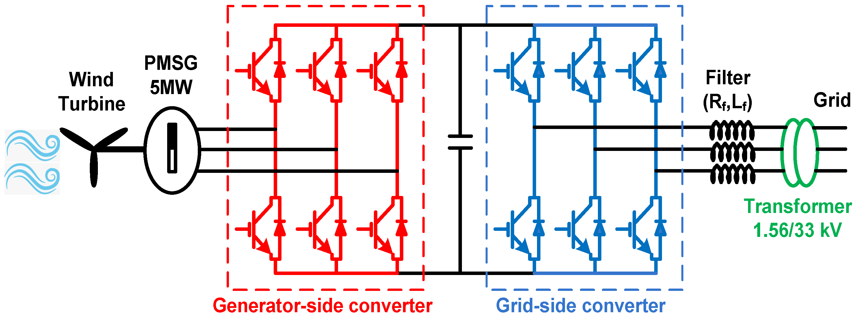
2. Model of the Wind Energy Conversion System

Figure 1 shows the structure of the wind energy conversion system. It consists of a WT and a PMSG, which is connected to the grid via a back-to-back converter. In the following, the model of each part is presented.

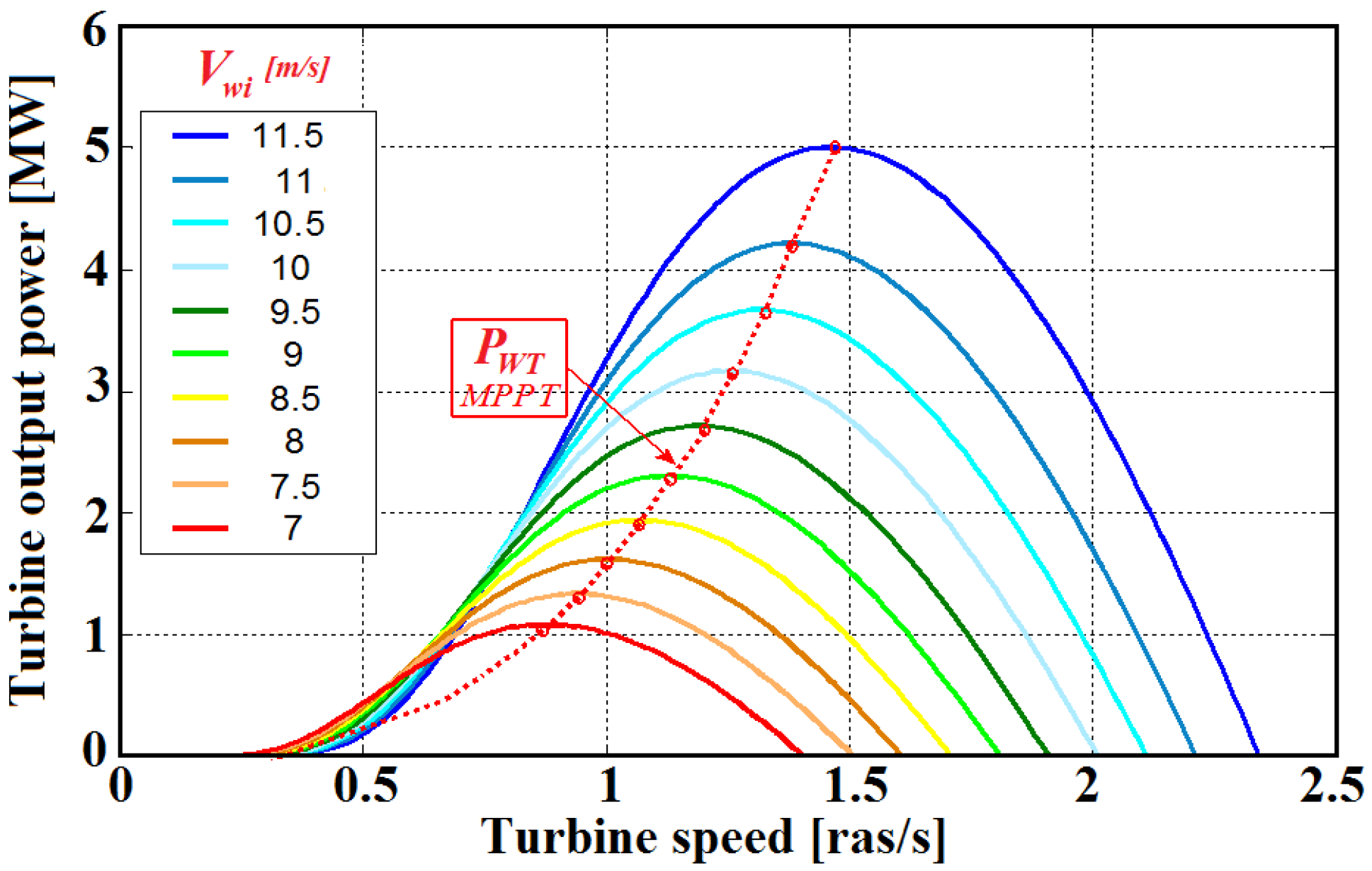
2.1. Wind Turbine Model

Different models have been proposed for wind turbines by researchers. In [28], a nonlinear model for a WT including the dynamics of the drivetrain was developed with emphasis on the modeling of the backlash phenomenon. In this paper, a simple common model is presented for the wind turbine. The aerodynamic power converted by the wind turbine depends on the power coefficient C_p, as presented in Equation (1) [29].

$$P_{WT}=\frac{1}{2}\rho \pi R^2{C}_p\left(\mathsf{\lambda },\mathsf{\beta }\right){V_{wi}}^3$$

(1)

where $\rho$ is the air density (1.225 kg/m³), $R$ stands for the radius of the rotor blade in (m), $V_{wi}$ represents the wind speed in (m/s), $\mathsf{\lambda }$ is the tip speed ratio (TSR) of the rotor blade, and $\mathsf{\beta }$ represents the blade pitch angle in (deg). The TSR is calculated by Equation (2) [30].

$$\mathsf{\lambda }=\frac{R{\Omega }_{gen}}{V_{wi}}$$

(2)

where ${\Omega }_{gen}$ is the angular speed of the wind turbine shaft in (rad/s).

The power coefficient is given by expression (3) [31,32]:

$$C_p\left(\mathsf{\lambda },\mathsf{\beta }\right)=0.5176\left(\frac{116}{{\mathsf{\lambda }}_i}-0.4\mathsf{\beta }-5\right)e^{\frac{-21}{{\mathsf{\lambda }}_i}}+0.0068{\mathsf{\lambda }}_i$$

(3)

In this equation, λ_i is calculated by Equation (4).

$${\mathsf{\lambda }}_i={\left(\frac{1}{\mathsf{\lambda }+0.08\mathsf{\beta }}-0\frac{0.035}{{\mathsf{\beta }}^3+1}\right)}^{-1}$$

(4)

2.2. Model of Permanent Magnet Synchronous Generator (PMSG)

The usual model of the PMSG is obtained by considering only the fundamental harmonic of the flux distribution in the air gap of the machine [5]. To define easily the control strategy of the system, the analytical model of the PMSG related to the rotor reference is given in Equation (5). In this equation, $V_{ds}$ and $V_{qs}$ are d-q axis voltages, $I_{ds}$ and $I_{qs}$ represent d-q axis currents, $L_d$ and $L_q$ stand for d-q axis inductances, $R_s$ is the stator phase resistance, and ${\psi }_f$ represents the magnet flux linkage [5].

$$\left[\begin{array}{c}{V}_{ds}\\ V_{qs}\end{array}\right]=\left[\begin{array}{cc}{R}_s+L_{d}s& -{\omega }_s{L}_q\\ {\omega }_s{L}_d& R_s+L_{q}s\end{array}\right]\left[\begin{array}{c}{I}_{ds}\\ I_{qs}\end{array}\right]+\left[\begin{array}{c}0\\ {\omega }_s{\psi }_f\end{array}\right]$$

(5)

The electromagnetic torque is expressed by Equation (6) [29].

$$T_{em}=\frac{3}{2}p\left[{\psi }_f+\left(L_d-L_q\right)I_{ds}\right]I_{qs}$$

(6)

2.3. Voltage Source Converter (VSC)

As it can be seen in Figure 1, the VSC is composed of two back-to-back three-phase IGBT bridges. Each one contains six switches. Neglecting the power losses in the converters and using the notation of Figure 2, the DC bus is modeled by Equation (7), in which P_WT and P_dc are the WT output active power and the power delivered to the network, respectively.

$$\frac{d{V}_{dc}}{dt}=\frac{1}{C_{dc}{V}_{dc}}\left(P_{WT}-P_{dc}\right)$$

(7)

Therefore, the input current of the grid-side converter, I₂, is calculated by Equation (8).

$$I_2=\frac{P_{WT}}{V_{dc}}-\frac{d{V}_{dc}}{dt}$$

(8)

In the next sections, two methods are explained to control the DC-bus voltage and each bridge.

2.4. Model of the Electrical Grid

The dynamic model of the electrical grid can be expressed by Equation (9), where $L_g$ and $R_g$ are the filter inductance and resistance, respectively, $V_{gd}$ and $V_{gq}$ present the d-q components of the grid voltage, $V_{id}$ and $V_{iq}$ stand for the d-q components of the inverter output voltage, $I_{gd}$ and $I_{gq}$ are the d-q axis components of the current measured on the grid, and $w_g$ is the fundamental frequency [2].

$$\{\begin{array}{c}{V}_{gd}=V_{id}-R_g{I}_{gd}-L_g\frac{d{I}_{gd}}{dt}+{\omega }_g{L}_g{I}_{gq}\\ V_{gq}=V_{iq}-R_g{I}_{gq}-L_g\frac{d{I}_{gq}}{dt}-{\omega }_g{L}_g{I}_{gd}\end{array}$$

(9)

The active and reactive powers injected to the grid are written as follows [17]:

$$\{\begin{array}{c}{P}_g=\frac{3}{2}(V_{gd}{I}_{gd}+V_{gq}{I}_{gq})\\ Q_g=\frac{3}{2}(V_{gq}{I}_{gd}-V_{gd}{I}_{gq})\end{array}$$

(10)

After developing the mathematical model of the system, two different control methods, a field-oriented control (FOC) and a flatness-based control (FBC) method, are explained in the following.

3. Field-Oriented Control Method

The converter connected to the stator of the machine controls the rotation speed of the generator and hence its torque. The used converter in the grid side ensures the DC-bus control and the active and reactive power management between the generator and the grid. This interface provides a nearly complete decoupling between the grid and the generator. To control the active power, the authors of [33] studied a method based on turbine stability-constrained available wind power. However, in this paper, the Maximum Power Point Tracking (MPPT) mode is studied, in which the wind speed is lower than the nominal speed $V_{wi-nom}$, which corresponds to the nominal power of the PMSG. In this operation mode, the angular speed $\Omega$ of the WT axis is controlled to follow the optimum value ${\Omega }_{opt}$ at which the power captured by the WT is maximum (as shown in Figure 3) and the pitch angle is equal to zero [34]. It should be mentioned that in overspeed operation mode, the pitch angle is controlled such that the power extracted from the wind is limited to its nominal value. For this purpose, different techniques have been proposed in the literature such as neuro-estimators, PI-controllers, and independent pitch control [35,36]. In the following, the principle of each power converter (Figure 1) control approach is explained.

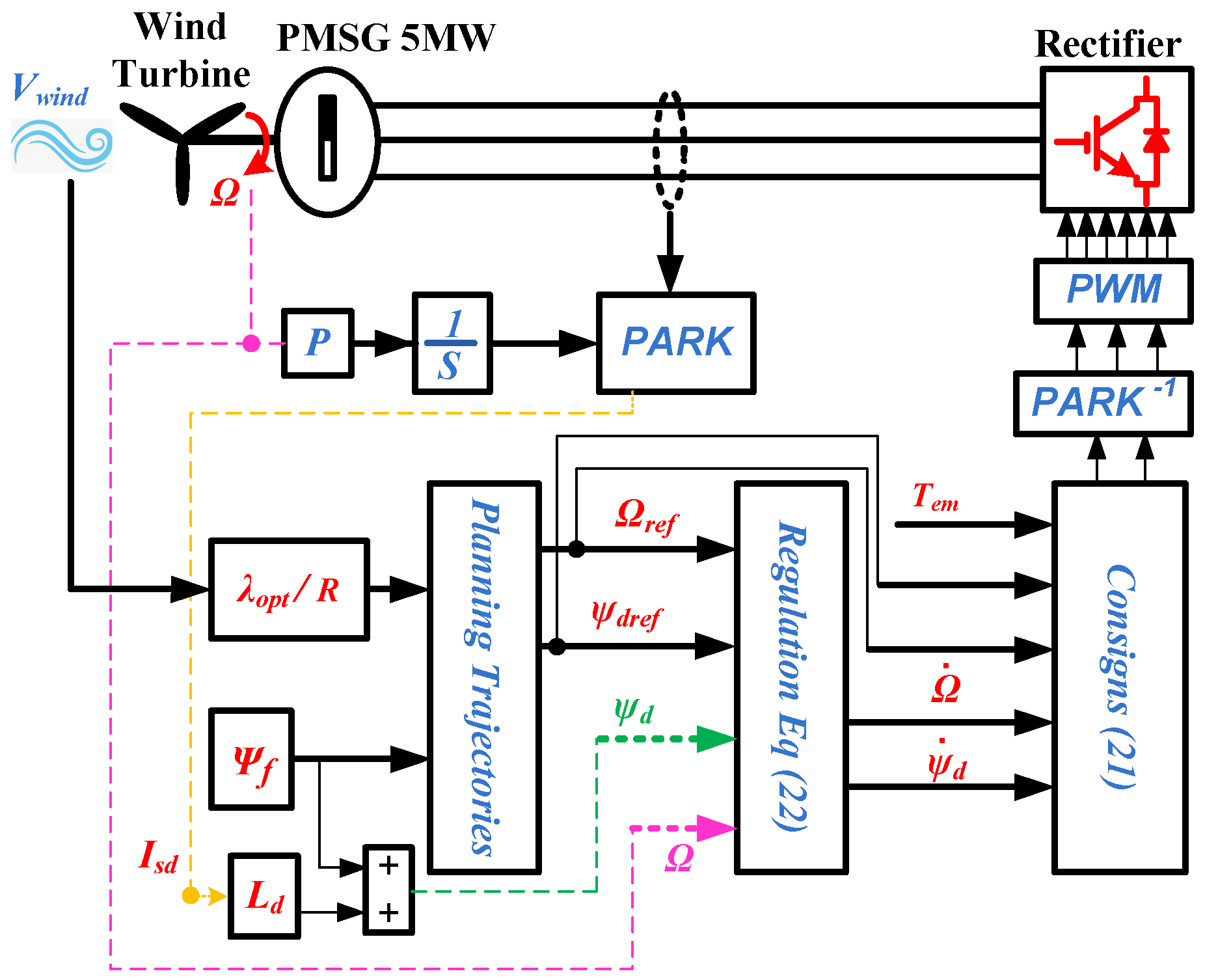
3.1. Wind Generator Control Method

The principle of the field-oriented control method is nowadays a standard way to control wind generators [5,37]. The control structure of the generator-side converter is shown in Figure 4. It consists of rotation speed control and the dq components of the generator stator current, which are explained in detail.

3.1.1. Rotation Speed Control

As mentioned above, the speed rotation is controlled to extract the maximum power existing in the wind turbine. The reference of the speed is obtained by the curves presented in Figure 3. The speed rotation control is carried out by a PI controller, which generates a reference value for the electromagnetic torque.

3.1.2. Stator’s Current Control

To control the dq components of the PMSG current, the reference values should be defined first. For this purpose, the reference value of the d-component of the current, I_sd-ref, is set to zero. This allows the reduction in the ohmic losses. Therefore, the electromagnetic torque expressed in Equation (6) is simplified as Equation (11).

$$T_{em}=\frac{3}{2}p{\Psi }_f{I}_{sq}$$

(11)

It was noted that the output of the speed controller is considered as the reference value for the electromagnetic torque. Therefore, the q-component of the current, I_sq-ref, is obtained using the output of the controller and Equation (11). Equation (12) presents the reference value of the dq components of the current.

$$\{\begin{array}{l}{I}_{sd-ref}=0\hfill \\ I_{sq-ref}=\frac{2}{3p{\Psi }_f}{T}_{em-ref}\hfill \end{array}$$

(12)

PI regulators are employed to control the dq components of the PMSG current, as shown in Equation (13).

$$\{\begin{array}{c}{v}_{sd-ref}=k_{pd}\left(I_{sd-ref}-I_{sd}\right)+k_{id}{\displaystyle \int }\left(I_{sd-ref}-I_{sd}\right)dt\\ v_{sq-ref}=k_{pq}\left(I_{sq-ref}-I_{sq}\right)+k_{iq}{\displaystyle \int }\left(I_{sq-ref}-I_{sq}\right)dt\end{array}$$

(13)

It is clear that the dynamics of the inner control loop (stator current) should be faster than that of the outer speed loop.

Figure 4 shows the block diagram of the explained wind generator control strategy.

3.2. Energy Management between the PMSG and the Grid

Energy management between the PMSG and the Grid includes two separated control loops, and each loop contains an inner current control one. More precisely, the outer loops control the DC-bus voltage and the reactive power, while the concerned inner loops control the d-component and the q-component of the grid current, respectively. The control block diagram is shown in Figure 5.

The active and reactive power can be estimated, as presented in Equation (10), by neglecting the power losses in the converters. To deliver the produced power to the grid, a Phase-Locked Loop (PLL) should be used to synchronize the output voltage of the inverter with the grid’s frequency. Figure 6 presents the PLL block diagram. The PLL imposes the $V_{gq}$ voltage to zero, which allows the decoupling of active and reactive power as written in (14).

$$\{\begin{array}{l}{P}_g=\frac{3}{2}{V}_{gd}{I}_{gd}\hfill \\ Q_g=-\frac{3}{2}{V}_{gd}{I}_{gq}\hfill \end{array}$$

(14)

By neglecting the power losses in the grid-side converter, the relationship between the active power exchanged between the grid and the DC bus is given by Equation (15).

$$V_{dc}·I_2=\frac{3}{2} V_{gd}·I_{gd}$$

(15)

where $I_2$ is the input current of the inverter.

In the following, the control strategy that manages the energy between the PMSG and the Grid is explained in detail.

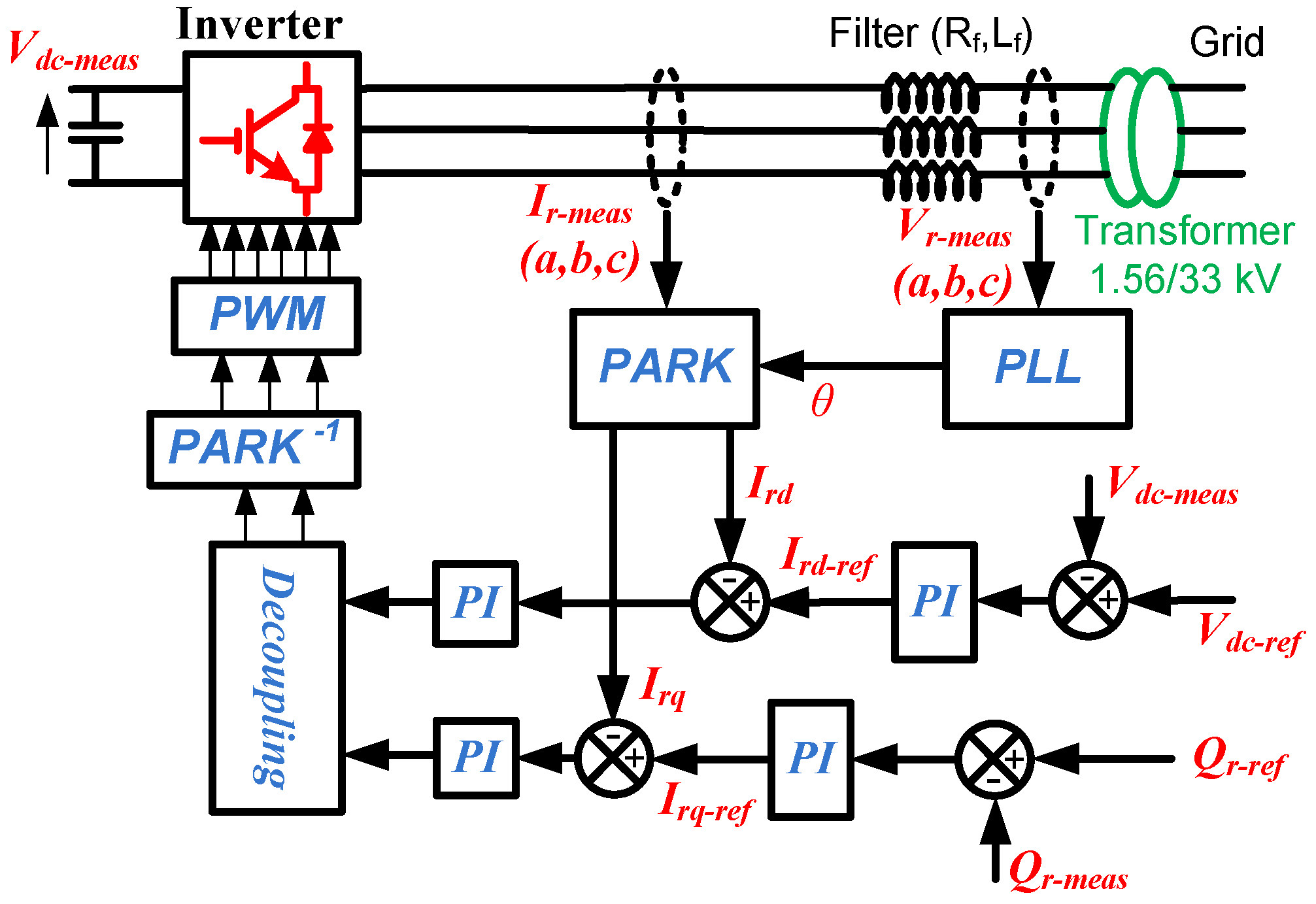
3.2.1. DC-Bus Voltage and Reactive Power Control

In order to ensure that the DC-bus voltage, V_dc, follows its reference, V_dc-ref, which is fixed at 4700 V, a PI controller is used. The same type of regulator is utilized to control the reactive power. The reference value of the reactive power is defined online depending on the grid conditions during the time. Therefore, the reactive power may be injected to the grid or be absorbed from the grid. Therefore, the controllers of the outer loops are presented by Equation (16).

$$\{\begin{array}{l}{I}_{gd-ref}=k_{pDC}\left(V_{dc-ref}-V_{dc}\right)+k_{iDC}{\displaystyle \int }\left(V_{dc-ref}-V_{dc}\right)dt\hfill \\ I_{gq-ref}=k_{pQ}\left(Q_{g-ref}-Q_g\right)+k_{iQ}{\displaystyle \int }\left(Q_{g-ref}-Q_g\right)dt\hfill \end{array}$$

(16)

3.2.2. Grid’s Currents Control

As it is shown in Equation (16), the d-axis current reference $I_{gd-ref}$ is obtained by the output of the DC-bus regulator, and the q-axis current reference $I_{gq-ref}$ is generated by the output of reactive power regulator. Again, a simple PI regulator can control the dq components of the grid’s current. Equation (17) presents outputs of the controllers.

$$\{\begin{array}{c}{V}_{gd-ref}=k_{pdg}\left(I_{gd-ref}-I_{gd}\right)+k_{idg}{\displaystyle \int }\left(I_{gd-ref}-I_{gd}\right)dt\\ V_{gq-ref}=k_{pqg}\left(I_{gq-ref}-I_{gq}\right)+k_{iqg}{\displaystyle \int }\left(I_{gq-ref}-I_{gd}\right)dt\end{array}$$

(17)

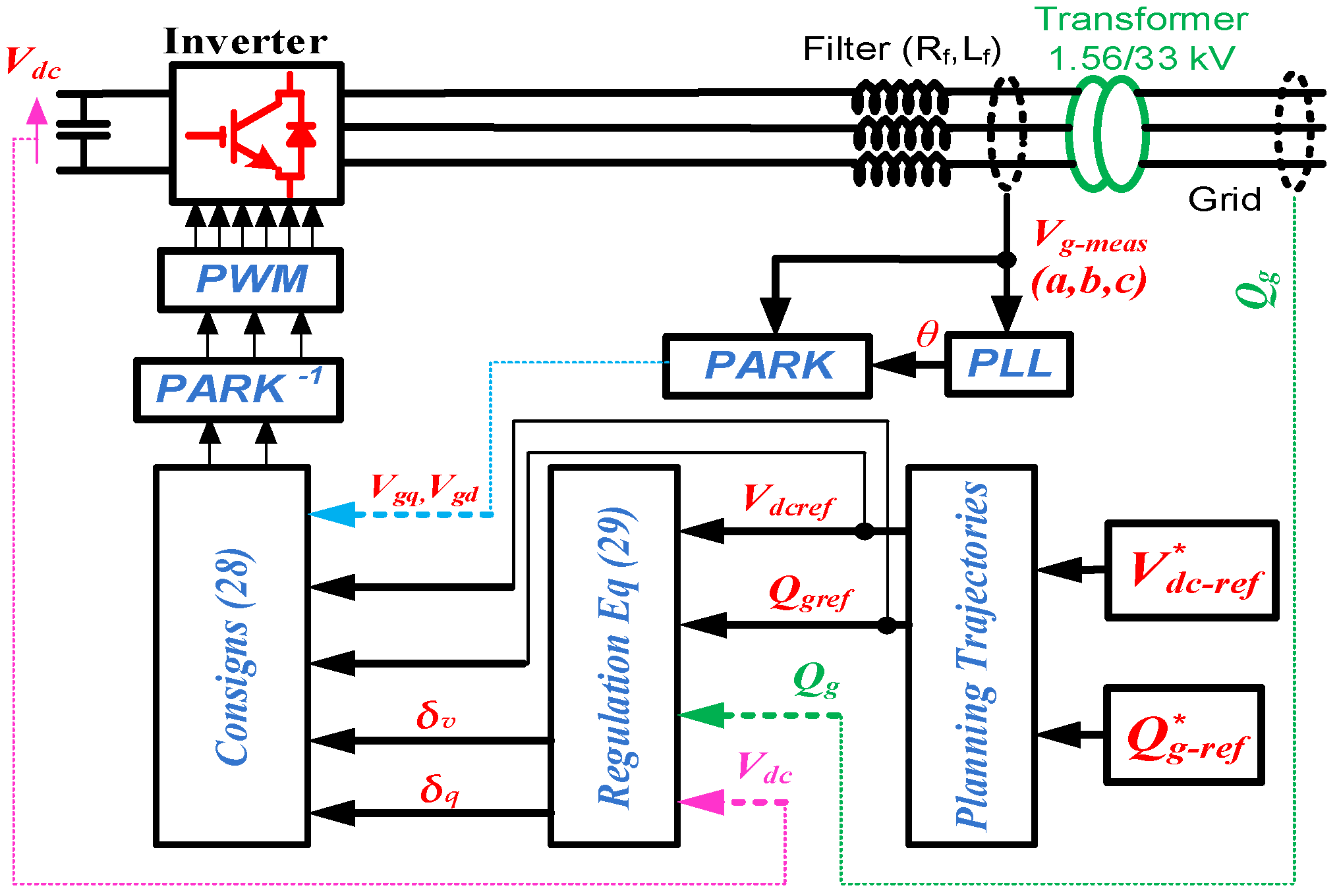
4. Flatness-Based Control

The property of flatness can be used to design control algorithms. A dynamic system is flat if and only if the state and control variables of the system can be written as functions of the flat output and its derivatives [38,39]. Mathematically, a system defined by: ẋ = f(x, u) (x ϵ Rⁿ and u ϵ R^m are state and the input vector, respectively) is considered to be differentially flat if an output y ϵ R^m can be found in the form of (18) such that the state and the input vectors be written like Equation (19) [38,39].

$$y=\phi \left(x,u,\dot{u},\dots ,u^{\left(q\right)}\right)$$

(18)

$$\{\begin{array}{l}x=\varphi \left(y,\dot{y},\dots ,y^{\left(r\right)}\right)\hfill \\ u=\zeta \left(y,\dot{y},\dots ,y^{\left(r+1\right)}\right)\hfill \end{array}$$

(19)

with rank (φ) = m, rank ($\zeta$) = m, and rank (ϕ) = n.

Generally, the control structure consists of a feedforward and a feedback part. As flatness allows for calculating the control inputs as functions of only the flat outputs, it can be used to design the feedforward part even for nonlinear systems. Therefore, to control a system, the appropriate output variables should be chosen first, and then the reference trajectories should be planned on them to calculate the control variable components.

To prove that the system is flat, it is divided by two subsystems, and it is shown that both subsystems are flat.

4.1. Wind Generator Control Method

Choosing the flux ${\psi }_d$ and the rotation speed $\Omega$ as the flat outputs of the first subsystem, the state variables of the system can be obtained from the mechanical and flux equation, as shown in Equation (21).

$$\{\begin{array}{l}{I}_{sd}=\frac{{\psi }_d-{\psi }_f}{L_d}={\varphi }_{I_{sd}}\left({\psi }_d\right)\hfill \\ I_{sq}=\frac{1}{p{\psi }_f}\left(J\dot{\Omega }+T_{em}+f\Omega \right)={\varphi }_{I_{sq}}\left(\Omega ,\dot{\Omega }\right)\hfill \end{array}$$

(20)

The control variables can also be written as Equation (21) using the model of the PMSG.

$$\{\begin{array}{l}{V}_{sd}=R_s{I}_{sd}+L_d\frac{d{I}_{sd}}{dt}-p\Omega L_q{I}_{sq}={\zeta }_{V_{sd}}\left({\psi }_d,\dot{{\psi }_d},\Omega ,\dot{\Omega }\right)\hfill \\ V_{sq}=R_s{I}_{sq}+L_q\frac{d{I}_{sq}}{dt}+p\Omega \left(L_d{I}_{sd}+{\psi }_f\right)={\zeta }_{V_{sq}}\left(\Omega ,\dot{\Omega },\ddot{\Omega },{\psi }_d\right)\hfill \end{array}$$

(21)

Therefore, the first subsystem is flat. To generate the reference trajectories of the system outputs, the optimum speed ${\Omega }_{opt}$ obtained from (2) is used. The optimum speed is calculated by replacing $\mathsf{\lambda }$ by ${\mathsf{\lambda }}_{opt}$, where ${\mathsf{\lambda }}_{opt}$ is the optimum TSR at which the power coefficient is maximum $C_{p-max}$. Therefore, the optimal speed is taken into account to generate the reference trajectory of $\Omega$. To control the dynamics of the output variables, a second-order filter is put on the references’ trajectories.

Concerning the second output variable, the constant flux linkage produced by the permanent magnets ${\psi }_f$ is considered as the reference value of ${\psi }_d$. Therefore, an online and an offline reference trajectory is designed for the system outputs, $\Omega$ and ${\psi }_d$, respectively.

In order to ensure tracking of the system outputs toward their own reference trajectories, ${\psi }_{dref}$ and ${\Omega }_{ref}$, a state feedback controller is used such as Equation (22).

$$\{\begin{array}{l}\left({\ddot{\Omega }}_{ref}-\ddot{\Omega }\right)+k_{\Omega 1}\left({\dot{\Omega }}_{ref}-\dot{\Omega }\right)+k_{\Omega 2}\left({\Omega }_{ref}-\Omega \right)+k_{\Omega 3}{\displaystyle \int }\left({\Omega }_{ref}-\Omega \right)dt=0\hfill \\ \left({\dot{\psi }}_{dref}-{\dot{\psi }}_d\right)+k_{\psi 1}\left({\psi }_{dref}-{\psi }_d\right)+k_{\psi 2}{\displaystyle \int }\left({\psi }_{dref}-{\psi }_d\right)dt=0\hfill \end{array}$$

(22)

The integral components are introduced to ensure a zero static error in the steady state and to compensate effects introduced by modeling errors. Substituting $\ddot{\Omega }$ and $\dot{{\psi }_d}$ obtained by the regulators in Equation (22) leads to the calculation of the control variables. These control variables are used to generate the switching signals of the wind turbine-side AC/DC converter.

To design the controller parameters, it is mentioned that Equation (22) has a cubic (first equation) and a quadratic (second equation) equation form where the variable is the error between the system output variable and their respective references. More precisely, Equation (22) can be written as Equation (23) in which ${\epsilon }_{\Omega }={\Omega }_{ref}-\Omega$ and ${\epsilon }_{{\psi }_d}={\psi }_{dref}-{\psi }_d$.

$$\{\begin{array}{l}{\stackrel{⃛}{\epsilon }}_{\Omega }+k_{\Omega 1}{\ddot{\epsilon }}_{\Omega }+k_{\Omega 2}{\dot{\epsilon }}_{\Omega }+k_{\Omega 3}{\epsilon }_{\Omega }=0\hfill \\ {\ddot{\epsilon }}_{{\psi }_d}+k_{\psi 1}{\dot{\epsilon }}_{{\psi }_d}+k_{\psi 2}{\epsilon }_{{\psi }_d}=0\hfill \end{array}$$

(23)

This contains a third-order and a second-order equation. An optimum choice for the parameters of the first one (third-order equation) is obtained by the factor theorem with pre-specified root locations in order to obtain a behavior close to that of the second-order. Therefore, the characteristic polynomial P(s) deduced from Equation (23) will be:

$$\{\begin{array}{l}P\left(s\right)=\left(s+p_{\Omega }\right)·\left(s^2+2{\xi }_{\Omega }{\omega }_{\Omega }s+{{\omega }_{\Omega }}^2\right)\hfill \\ P\left(s\right)=s^2+2{\xi }_{{\psi }_d}{\omega }_{{\psi }_d}s+{{\omega }_{{\psi }_d}}^2\hfill \end{array}$$

(24)

The equivalent of Equations (23) and (24) leads to the calculation of the controller parameters, which are shown in Equations (25) and (26).

$$\{\begin{array}{l}{k}_{\Omega 1}=2 {\xi }_{\Omega } {\omega }_{\Omega }-p_{\Omega }\hfill \\ k_{\Omega 2}={{\omega }_{\Omega }}^2-2 {\xi }_{\Omega } p_{\Omega } {\omega }_{\Omega }\hfill \\ k_{\Omega 3}=p_{\Omega }{{\omega }_{\Omega }}^2\hfill \end{array}$$

(25)

ξ_Ω and ω_Ω represent the damping ratio and the cut-off pulsations of the speed loop, respectively. These values are chosen to ensure a well-damped response and an appropriate fast transient response. In the same way, the parameters of the flux loop controller (the second relation of Equation (22)) are obtained as:

$$\{\begin{array}{l}{k}_{\psi 1}=2 {\xi }_{{\psi }_d}{\omega }_{{\psi }_d}\hfill \\ k_{\psi 2}={{\omega }_{{\psi }_d}}^2\hfill \end{array}$$

(26)

Again, ${\xi }_{{\psi }_d}$ and ${\omega }_{{\psi }_d}$ represent the damping ratio and the cut-off pulsations of the flux loop, respectively.

Figure 7 shows the block diagram of the explained control method for the wind generator.

4.2. Energy Management between the PMSG and the Grid

As mentioned before, the grid-side converter is controlled such that the DC-bus voltage and the reactive power can be managed. Therefore, these two variables, i.e., the DC-bus voltage $V_{dc}$ and the reactive power $Q_g$, are considered as vector components of the second subsystem output. By substituting I₂ from Equation (8) in Equation (15), and by using Equation (14), the state variables of the second subsystem, I_gd and I_gq, can be written as functions of the subsystem flat outputs, as presented by Equation (27).

$$\{\begin{array}{l}{I}_{gd}=\frac{2}{3·V_{gd}}\left(P_{WT}-C_{dc}{V}_{dc}\frac{d{V}_{dc}}{dt}\right)={\varphi }_{I_{gd}}\left(V_{dc},{\dot{V}}_{dc}\right)\hfill \\ I_{gq}=\frac{-2}{3·V_{gd}}{Q}_g={\varphi }_{I_{gq}}\left(Q_g\right)\hfill \end{array}$$

(27)

In addition, $V_{id}$ and $V_{iq}$, the d-q components of the inverter output voltage, are chosen as the control variables of the second subsystem, which can be written as functions of second subsystem flat outputs and their derivatives. They are expressed by Equation (28).

$$\{\begin{array}{c}{V}_{id}=V_{gd}+R_g{I}_{gd}+L_g\frac{d}{dt}{I}_{gd}-{\omega }_{g }{L}_{g }{I}_{gq}={\zeta }_{V_{id}}\left(V_{dc},{\dot{V}}_{dc},{\ddot{V}}_{dc},Q_g\right)\\ V_{iq}=V_{gq}+R_g{I}_{gq}+L_g\frac{d}{dt}{I}_{gq}+{\omega }_{g }{L}_{g }{I}_{gd}={\zeta }_{V_{iq}}\left(V_{dc},{\dot{V}}_{dc},Q_g,{\dot{Q}}_g\right)\end{array}$$

(28)

Therefore, the second subsystem is also flat.

Before controlling the output variables $V_{dc}$ and $Q_g$, the reference values should be defined. The same values explained in the third section are considered as the reference values to let everyone compare the behavior of the system under the two control methods. It should be mentioned that a filter may be applied to the system outputs to force the system to follow a desired dynamic. Furthermore, this can protect the system against the rapid changes in system variables. A state feedback controller shown in Equation (29) guarantees the output tracking of the defined reference.

$$\{\begin{array}{l}0=\left({\ddot{V}}_{dcref}-{\ddot{V}}_{dc}\right)+k_{d1}·\left({\dot{V}}_{dcref}-{\dot{V}}_{dc}\right)+k_{d2}·\left(V_{dcref}-V_{dc}\right)\hfill \\ +k_{d3}·{{\displaystyle \int }}^{}\left(V_{dcref}-V_{dc}\right)dt\hfill \\ 0=\left({\dot{Q}}_{gref}-{\dot{Q}}_g\right)+k_{q1}·\left(Q_{gref}-Q_g\right)+k_{q2}·{{\displaystyle \int }}^{}\left(Q_{gref}-Q_g\right)dt\hfill \end{array}$$

(29)

The same method explained in Section 4.1 is used to calculate the controllers’ parameters. By substituting the outputs of controllers of Equation (29), δ_v $={\ddot{V}}_{dc}$ and δ_q = ${\dot{Q}}_g$, in Equation (28), the control variables of the second subsystem are calculated. The inverse park transformation and well-known PWM are used to finally generate the switching signals of the inverter.

Figure 8 shows the block diagram of the control method applied to the second subsystem.

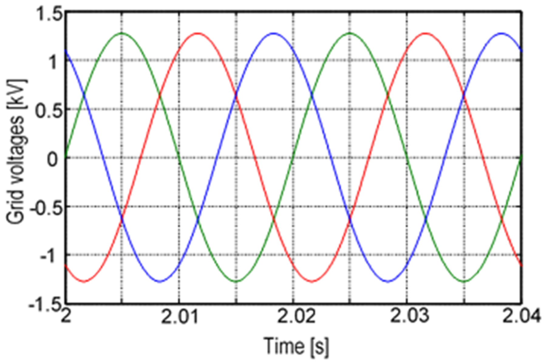
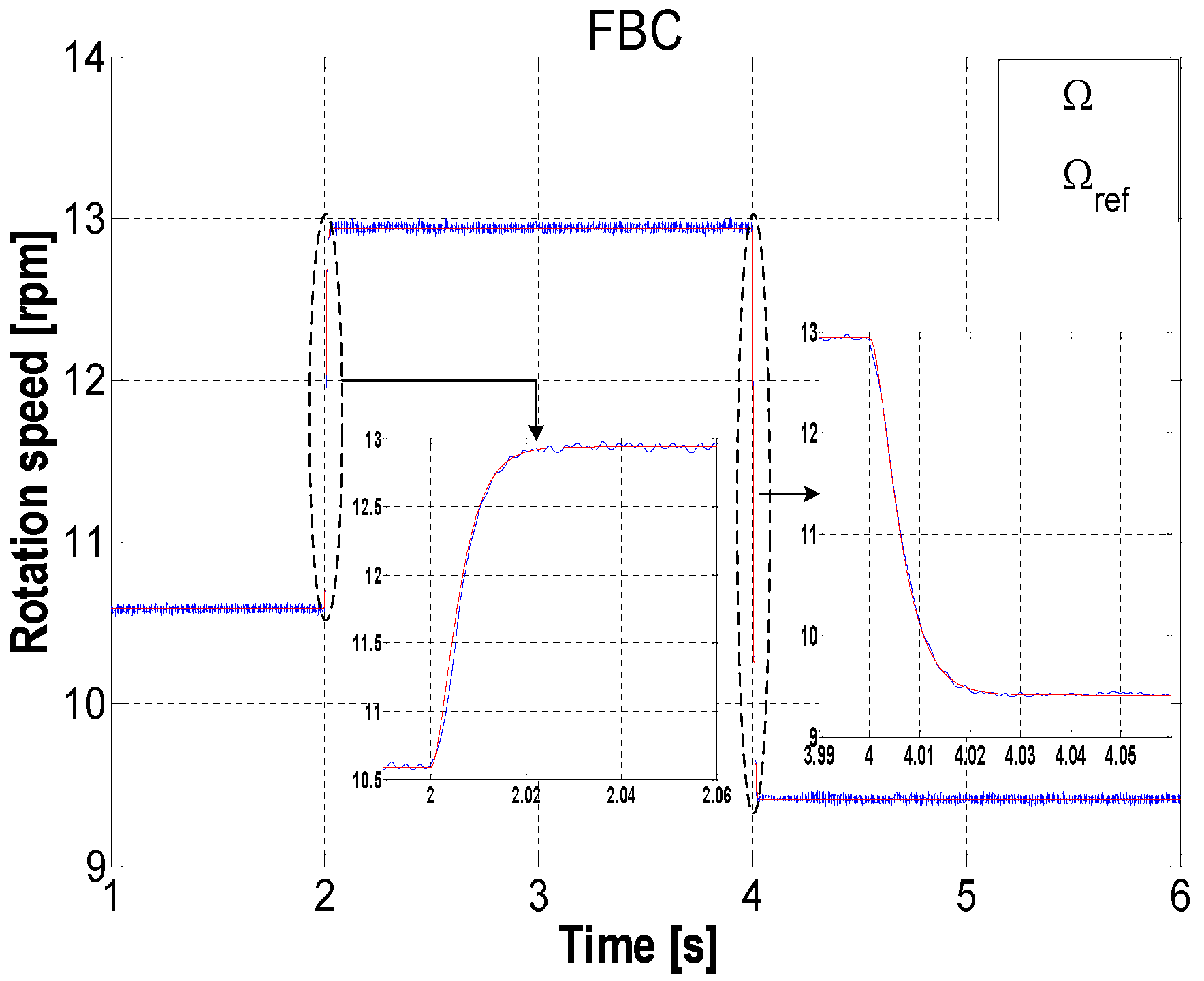
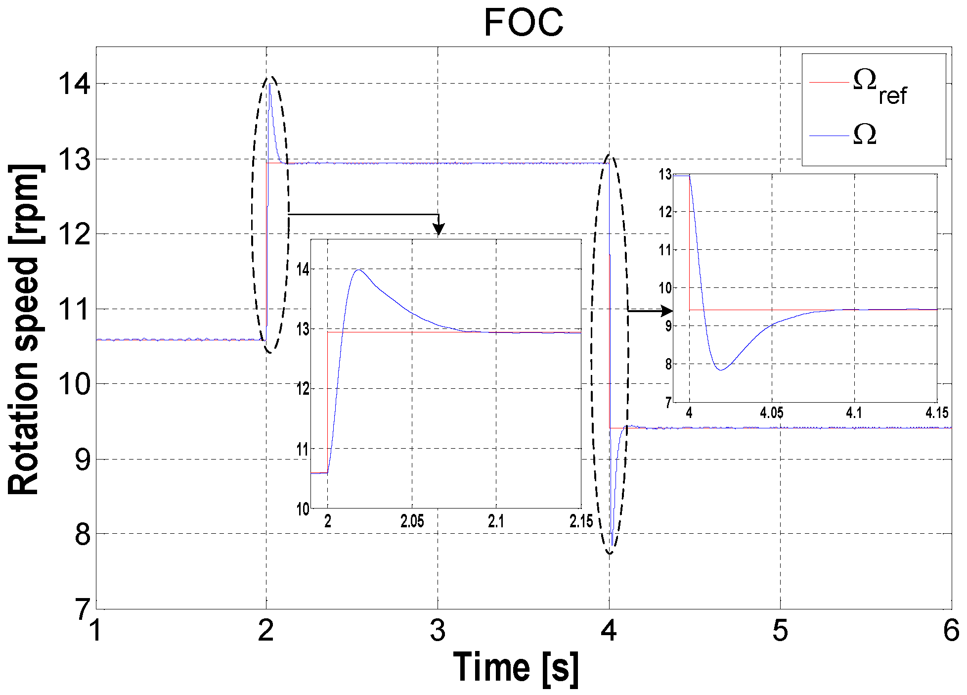
5. Simulation Results and Discussion

To validate the applied control methods, FOC and FBC, and to be able to compare the system performance with the applied control strategies, the system presented in Figure 1 is modeled in a SimPowerSystems environment in Matlab with the parameters listed in

Table 1. System parameters.

Parameter	Value
Pn	5 MW
R	56 M
Rs	6.25 mΩ
J	104 kg·m2
Vdcref	4700 V
Number of blades	3
Ls	4.23 mH
${\psi }_f$	11.15 Nm/A
Cdc	0.04 mF
Lf	0.5 mH

. It presents the wind turbine, the PMSG, the DC bus, and the filter parameters.

As it can be seen from Figure 5 or Figure 8, the energy conversion system is connected to the grid through a 1.56/33 KV transformer. Figure 9 displays a three-phase set of line-to-neutral voltages for the primary side of the transformer. To compare the dynamic performance of the conventional (FOC) and the proposed (FBC) control methods with this connection, a positive wind speed step variation from 9 m/s to 11 m/s and a negative one from 11 m/s to 8 m/s are applied to the system at t = 2 s and t = 4 s, respectively. Two parameters are measured then for the output variables: settling time and overshoot.

Figure 10 and Figure 11 show the rotation speed of the PMSG obtained with FBC and FOC methods, respectively, in which reference values of the DC-bus voltage and reactive power remain constant ($V_{dcref}$ = 4700 V and $Q_{gref}$ = 0 VAR). It should be mentioned that the wind turbine is controlled to extract the maximum power from the wind for both control methods. Therefore, the reference value for the rotation speed is generated by the MPPT strategy by using Figure 3 for each wind speed. In the studied case, this reference value has a positive step change from almost 10.6 RPM to 12.9 RPM and a negative step change from 12.9 RPM to 9.4 RPM. Although the rotation speed is well regulated with both methods, the machine speed controlled by the FOC method has a significant overshoot during the wind speed variations. The overshoot measured for the FOC is more than 40%, while there is not any overshoot by using the FBC method. Furthermore, the second method (FBC) has a lower settling time, which means the system controlled by the flatness-based method is faster than the other one. Indeed, the dynamics of the output variables are managed and controlled by a second-order filter put on the references’ trajectories in the FBC method. This leads to control of the output variables in the transient states, as well as the steady state. Therefore, the overshoot and the settling time can be designed favorably, which is the advantage of the FBC in comparison with the FOC. Furthermore, the system output follows perfectly its planned reference trajectory, which proves that the controller parameters are well calculated.

The active power (and mechanical power) curves of the system during the wind speed variations are presented in Figure 12 and Figure 13 for the system that is controlled by the FBC and FOC method, respectively. The simulation results show again that the system controlled by the FBC method has faster dynamics in comparison with the second one. More precisely, the settling time of the active power is almost 0.18 s with the FBC, while it is almost equal to 0.25 s with the FOC. Furthermore, the overshoot of the response is equal to 5% and 30% for the FBC and FOC, respectively. Indeed, the dynamics of the active power is indirectly controlled in the FBC. Therefore, it is expected that the dynamics of this variable is faster with a lower overshoot. Nevertheless, the efficiency of the system is almost the same for both control methods in steady states. That is because of the effectiveness of the controllers in both systems.

Relating to the second subsystem (grid-side converter that connects the DC bus to the grid), the DC-bus voltage and the reactive power should be controlled.

Figure 14 and Figure 15 show the DC-bus voltage control obtained with FBC and FOC methods, respectively. Although the DC-bus voltage, V_dc, is controlled well with both methods, the effect of wind speed variations on DC-bus voltage is much less with the FBC in comparison with the FOC. This is due to the faster dynamics of the PMSG, which is controlled by the FBC as mentioned above. It is mentioned that the reference value of the DC-bus voltage, V_dcref, is fixed to 4700 V.

For a better evaluation of the control performance of the DC-bus voltage, as well as modeling the DC-bus voltage variation due to the low-voltage ride-through (LVRT), a positive and a negative step variation are applied to the DC-bus voltage reference, V_dcref. Figure 16 and Figure 17 show the DC-bus voltage control obtained with FBC and FOC methods, respectively. As can be seen, although the DC-bus voltage is controlled well with both control strategies, the first one does not contain any overshoot, while utilizing the second one leads to a 25% overshoot. Furthermore, the FBC method results in a faster response. The settling time with FBC is 70 ms, while it is almost 450 ms with FOC. As with the first subsystem (PMSG side), the dynamics of the output variables are managed and controlled by a second-order filter put on the references’ trajectories in the FBC method. Furthermore, the dynamics of the PMSG is faster in the FBC method, which leads to a better control of the DC-bus voltage in both the transient and steady state.

Figure 18 and Figure 19 show the three-phase set of the system current, which is injected to the grid during the mentioned test. The effect of the smaller overshoot and settling time of the DC-bus voltage and the active power in the system controlled by the FBC is clear on the line currents. As it can be seen, the current behavior in the first case (system controlled by FBC) in the transient state is better than that of the second one (system controlled by FOC). Again, this is result of the better control dynamics of the system with the FBC method. The zoomed injected currents into the grid are presented in Figure 20.

Concerning the reactive power, two tests are carried out to show the performance of the control methods. To study the dynamic behavior, the system response to reactive power reference variations from 1 MVAr to 2 MVAr and from 2 MVAr to 0 MVAr obtained by the FBC and FOC method is presented in Figure 21 and Figure 22, respectively. These figures show that the dynamics of the reactive power variation in the system with both control methods are almost the same. These results are predictable as the reactive power is controlled independently. More precisely, the reactive power is injected directly into the electrical network with infinite dynamics.

In Section 3 and Section 4, it is mentioned that the reference value of the reactive power is defined online depending on the grid conditions. Therefore, the reactive power may be injected into the grid or be absorbed from the grid. To display the reactive power control ability in all situations, Figure 23 and Figure 24 show the control of the reactive power where the system is controlled by FBC and FOC, respectively. It can be seen clearly that the reactive power is well controlled by both control methods.

Table 2. Settling time comparison of some variables of the system controlled by FBC and FOC methods.

Variable	Response Time (ms)
	FBC Method	FOC Method
Rotation speed (Ω)	15	60
DC-bus voltage $(V_{dc}$)	70	450
Active power $(P_g$)	180	250
Reactive power $(Q_g$)	0.1	0.1

and

Table 3. Overshoot comparison of some variables of the system controlled by FBC and FOC methods.

Variable	Overshoot (%)
	FBC Method	FOC Method
Rotation speed (Ω)	0	40
DC-bus voltage $(V_{dc}$)	0	25
Active power $(P_g$)	5	30

compare and summarize the settling time and overshoot values measured from the simulation results for the mentioned system variables. It is noted that values measured for the DC-bus voltage are obtained for a direct step variation on its reference.

As a result, although both control strategies are efficient at managing the energy in the studied system, the FBC has better performances, especially in the transient state when the wind speed varies. This is proven by the simulation results for the worst case where the wind varies abruptly.

6. Conclusions

In this paper, a nonlinear control method called flatness-based control (FBC) is proposed for application to a wind energy conversion system based on a permanent magnet synchronous generator (PMSG). This variable-speed PMSG is connected to the grid via a back-to-back converter. The aim of this paper is to compare the system behavior with the conventional field-oriented control (FOC) method in which the maximum power is extracted from the wind. To compare the behavior of the system, the simulation results of the mathematical model of the system obtained by MATLAB/SimPowerSystems are presented. The results prove the effectiveness of both control methods to manage the energy in the studied system. However, the FBC performs better, especially in the transient state when the wind speed varies. More precisely, it is shown that the high bandwidth control method with only one closed-loop control based on the flatness properties results in less settling time and less overshoot in comparison with the FOC for the controlled variables, i.e., rotation speed of the PMSG and DC-bus voltage. In addition, the dynamic performance that is controlled by a filter put on the planned references trajectories in the FBC method can manage the output, control, and state variables in the transient states, as well as the steady states, taking into account the different constraints. Therefore, this method can be used to control the pitch angle of the wind turbine and to enhance the Primary Frequency Control (PFC) capability, as well as Low-Voltage Ride-Through (LVRT) capability, of an offshore wind farm connected to the grid.

References

1. Cordeiro-Costas, M.; Villanueva, D.; Feijóo-Lorenzo, A.; Martínez-Torres, J. Simulation of Wind Speeds with Spatio-Temporal Correlation. Appl. Sci. 2021, 11, 3355. [Google Scholar] [CrossRef]
2. Chavero-Navarrete, E.; Trejo-Perea, M.; Jáuregui-Correa, J.C.; Carrillo-Serrano, R.V.; Ronquillo-Lomeli, G.; Ríos-Moreno, J.G. Pitch Angle Optimization for Small Wind Turbines Based on a Hierarchical Fuzzy-PID Controller and Anticipated Wind Speed Measurement. Appl. Sci. 2021, 11, 1683. [Google Scholar] [CrossRef]
3. Lee, J.; Zhao, F. Global Wind Report 2019; GWEC Global Wind Energy Council: Brussels, Belgium, 2020. [Google Scholar]
4. Sun, M.; Min, Y.; Chen, L.; Hou, K.; Xia, D.; Mao, H. Optimal auxiliary frequency control of wind turbine generators and coordination with synchronous generators. CSEE J. Power Energy Syst. 2021, 7, 78–85. [Google Scholar]
5. Mansour, M.; Mansouri, M.; Mmimouni, M. Study and Control of a Variable-Speed Wind-Energy System Connected to the Grid. Int. J. Renew. Energy Res. 2011, 1, 96–104. [Google Scholar]
6. Guo, Y.; Gao, H.; Wu, Q.; Zhao, H.; Østergaard, J.; Shahidehpour, M. Enhanced Voltage Control of VSC-HVDC-Connected Offshore Wind Farms Based on Model Predictive Control. IEEE Trans. Sustain. Energy 2018, 9, 474–487. [Google Scholar] [CrossRef] [Green Version]
7. Zhang, Z.; Li, Z.; Kazmierkowski, M.; Rodríguez, J.; Kennel, R. Robust Predictive Control of Three-Level NPC Back-to-Back Power Converter PMSG Wind Turbine Systems With Revised Predictions. IEEE Trans. Power Electron. 2018, 33, 9588–9598. [Google Scholar] [CrossRef]
8. Zhao, H.; Wu, Q.; Guo, Q.; Sun, H.; Xue, Y. Distributed Model Predictive Control of a Wind Farm for Optimal Active Power ControlPart II: Implementation With Clustering-Based Piece-Wise Affine Wind Turbine Model. IEEE Trans. Sustain. Energy 2015, 6, 840–849. [Google Scholar] [CrossRef] [Green Version]
9. Shariatpanah, H.; Fadaeinedjad, R.; Rashidinejad, M. A New Model for PMSG-Based Wind Turbine with Yaw Control. IEEE Trans. Energy Convers. 2013, 28, 929–937. [Google Scholar] [CrossRef]
10. Ahmed, A.; Ran, L.; Bumby, J.R. New Constant Electrical Power Soft-Stalling Control for Small-Scale VAWT. IEEE Trans. Energy Convers. 2010, 25, 1152–1161. [Google Scholar] [CrossRef]
11. Soliman, M.; Hasanien, H.; Azazi, H.; El-Kholy, E.; Mahmoud, S. An Adaptive Fuzzy Logic Control Strategy for Performance Enhancement of a Grid-Connected PMSG-Based Wind Turbine. IEEE Trans. Ind. Inform. 2019, 15, 3163–3173. [Google Scholar] [CrossRef]
12. Yin, Y.; Liao, M.; Lyu, P. The dynamic stability analysis of wind turbines under different control strategies. In Proceedings of the 2015 IEEE 5th International Conference on Electric Utility Deregulation and Restructuring and Power Technologies (DRPT), Changsha, China, 26–29 November 2015. [Google Scholar]
13. Ikni, D.; Camara, M.B.; Payman, A.; Dakyo, B. Dynamic Control of Wind Energy Conversion System. In Proceedings of the 8th International Conference and Exhibition on Ecological Vehicles and Renewable Energies (EVER), Monaco, France, 27–30 March 2013. [Google Scholar]
14. González-Longatt, F.M.; Wall, P.; Terzija, V. A Simplified Model for Dynamic Behavior of Permanent Magnet Synchronous Generator for Direct Drive Wind Turbines. In Proceedings of the IEEE PES Trondheim PowerTech, Trondheim, Norway, 19–23 January 2011. [Google Scholar]
15. Chinchilla, M.; Arnaltes, S.; Burgos, J.C. Control of Permanent-Magnet Generators Applied to Variable-Speed Wind-Energy Systems Connected to the Grid. IEEE Trans. Energy Convers. 2006, 21, 130–135. [Google Scholar] [CrossRef] [Green Version]
16. Mahersi, E. The Wind energy Conversion System Using PMSG Controlled by Vector Control and SMC Strategies. Int. J. Renew. Energy Res. 2013, 3, 41–50. [Google Scholar]
17. Thakur, D.; Jiang, J. Control of a PMSG Wind-Turbine under Asymmetrical Voltage Sags Using Sliding Mode Approach. IEEE Power Energy Technol. Syst. J. 2018, 5, 47–55. [Google Scholar] [CrossRef]
18. Wang, C.; Liu, X. Sliding mode control for maximum wind energy capture of DFIG-based wind turbine. In Proceedings of the 2015 IEEE 27th Chinese Control and Decision Conference (CCDC), Qingdao, China, 23–25 May 2015. [Google Scholar]
19. Uehara, A.; Pratap, A.; Goya, T.; Senjyu, T.; Yona, A.; Urasaki, N.; Funabashi, T. A Coordinated Control Method to Smooth Wind Power Fluctuations of a PMSG-Based WECS. IEEE Trans. Energy Convers. 2011, 26, 550–558. [Google Scholar] [CrossRef]
20. Lyu, X.; Zhao, J.; Jia, Y.; Xu, Z.; Wong, K. Coordinated Control Strategies of PMSG-Based Wind Turbine for Smoothing Power Fluctuations. IEEE Trans. Power Syst. 2019, 34, 391–401. [Google Scholar] [CrossRef]
21. Luo, H.; Hu, Z.; Zhang, H.; Chen, H. Coordinated Active Power Control Strategy for Deloaded Wind Turbines to Improve Regulation Performance in AGC. IEEE Trans. Power Syst. 2019, 34, 98–108. [Google Scholar] [CrossRef]
22. Palejiya, D.; Chen, D. Performance Improvements of Switching Control for Wind Turbines. IEEE Trans. Sustain. Energy 2016, 7, 526–534. [Google Scholar] [CrossRef]
23. Payman, A.; Pierfederici, S.; Meibody-Tabar, F.; Davat, B. An Adapted Control Strategy to Minimize DC-Bus Capacitors of a Parallel Fuel Cell/Ultracapacitor Hybrid System. IEEE Trans. Power Electron. 2011, 26, 3843–3852. [Google Scholar] [CrossRef]
24. Battiston1, A.; Martin, J.; Miliani, E.; Nahid-Mobarakeh, B.; Pierfederici, S.; Meibody-Tabar, F. Control of a PMSM Fed by a Quasi Z-Source Inverter Based on Flatness Properties and Saturation Schemes. In Proceedings of the 15th European Conference on Power Electronics and Applications (EPE), Lille, France, 3–5 September 2013; pp. 1–10. [Google Scholar]
25. Delaleau, E.; Stankovic, A.M. Flatness-based hierarchical control of the PM synchronous motor. In Proceedings of the 2004 American Control Conference, Boston, MA, USA, 30 June–2 July 2004. [Google Scholar]
26. Margaris, I.D.; Papathanassiou, S.; Hatziargyriou, N.; Hansen, A.; Sørensen, P. Frequency Control in Autonomous Power Systems With High Wind Power Penetration. IEEE Trans Sustain. Energy 2012, 3, 189–199. [Google Scholar] [CrossRef]
27. Zhao, X.; Meng, L.; Dragicevic, T.; Savaghebi, M.; Guerrero, J.M.; Vasquez, J.C.; Wu, X. Distributed low voltage ride-through operation of power converters in grid-connected microgrids under voltage sags. In Proceedings of the Industrial Electronics Society, IECON 2015—41st Annual Conference of the IEEE, Yokohama, Japan, 9–12 November 2015; pp. 1909–1914. [Google Scholar]
28. Ghasemi, S.; Tabesh, A.; Askari-Marnani, J. Application of Fractional Calculus Theory to Robust Controller Design for Wind Turbine Generators. IEEE Trans. Energy Convers. 2014, 29, 780–787. [Google Scholar] [CrossRef]
29. Chavero-Navarrete, E.; Trejo-Perea, M.; Jáuregui-Correa, J.C.; Carrillo-Serrano, R.V.; Ronquillo-Lomeli, G.; Ríos-Moreno, J.G. Pitch Angle Optimization by Intelligent Adjusting the Gains of a PI Controller for Small Wind Turbines in Areas with Drastic Wind Speed Changes. Sustainability 2019, 11, 6670. [Google Scholar] [CrossRef] [Green Version]
30. Eisa, S.A. Modeling dynamics and control of type-3 DFIG wind turbines: Stability, Q Droop function, control limits and extreme scenarios simulation. Electr. Power Syst. Res. 2019, 166, 29–42. [Google Scholar] [CrossRef]
31. Dekali1, Z.; Baghli1, L.; Boumediene, A.; Djemai, M. Control of a Grid Connected DFIG Based Wind Turbine Emulator. In Proceedings of the 2018 IEEE 5th International Symposium on Environment-Friendly Energies and Applications (EFEA), Rome, Italy, 24–26 September 2018. [Google Scholar]
32. Llano, D.; McMahon, R.; Tatlow, M. Control algorithms for permanent magnet generators evaluated on a wind turbine emulator test-rig. In Proceedings of the 7th IET International Conference on Power Electronics, Machines and Drives (PEMD 2014), Manchester, UK, 8–10 April 2014. [Google Scholar]
33. Yin, M.; Xu, Y.; Shen, C.; Liu, J.; Dong, Z.Y.; Zou, Y. Turbine Stability-Constrained Available Wind Power of Variable Speed Wind Turbines for Active Power Control. IEEE Trans. Power Syst. 2017, 32, 2487–2488. [Google Scholar] [CrossRef]
34. Li, Y.; Xu, Z.; Meng, K. Optimal Power Sharing Control of Wind Turbines. IEEE Trans. Power Syst. 2017, 32, 824–825. [Google Scholar] [CrossRef]
35. Sierra-García, J.; Santos, M. Improving Wind Turbine Pitch Control by Effective Wind Neuro-Estimators. IEEE Access 2021, 9, 10413–10425. [Google Scholar] [CrossRef]
36. Wang, X.; Jiang, Z.; Lu, H.; Wang, X.; Meng, Y.; Li, S. Independent Pitch Control Strategy and Simulation for Reducing Unbalanced Load of Wind Turbine. In Proceedings of the 2020 IEEE 32th Chinese Control and Decision Conference (CCDC), Hefei, China, 22–24 August 2020. [Google Scholar]
37. Furmanik, M.; Gorel, L.; Konvicný, D.; Rafajdus, P. Comparative Study and Overview of Field-Oriented Control Techniques for Six-Phase PMSMs. Appl. Sci. 2021, 11, 7841. [Google Scholar] [CrossRef]
38. Fliess, M.; Lévine, J.; Martin, P.; Rouchon, P. Flatness and defect of non-linear systems: Introductory theory and examples. Int. J. Control 1995, 61, 1327–1361. [Google Scholar] [CrossRef] [Green Version]
39. Veeser, F.; Braun, T.; Kiltz, L.; Reuter, J. Nonlinear Modelling, Flatness-Based Current Control, and Torque Ripple Compensation for Interior Permanent Magnet Synchronous Machines. Energies 2021, 14, 1590. [Google Scholar] [CrossRef]
Figure 1. Structure of the wind energy conversion system.
Processes 10 00378 g001
Figure 2. DC bus in the back-to-back converter.
Processes 10 00378 g002
Figure 3. Maximum power according to the wind speeds.
Processes 10 00378 g003
Figure 4. Wind generator field-oriented control strategy.
Processes 10 00378 g004
Figure 5. Energy management between the PMSG and Grid with FOC method.
Processes 10 00378 g005
Figure 6. PLL block diagram.
Processes 10 00378 g006
Figure 7. Wind generator control method based on flatness property.
Processes 10 00378 g007
Figure 8. Energy management between the PMSG and Grid with FOC method.
Processes 10 00378 g008
Figure 9. The measured voltages of the grid in the primary side of the transformer.
Processes 10 00378 g009
Figure 10. Rotation speed of the PMSG obtained with FBC method.
Processes 10 00378 g010
Figure 11. Rotation speed of the PMSG obtained with FOC method.
Processes 10 00378 g011
Figure 12. Active power response obtained with the FBC method.
Processes 10 00378 g012
Figure 13. Active power response obtained with the FOC method.
Processes 10 00378 g013
Figure 14. DC-bus voltage obtained with FBC method.
Processes 10 00378 g014
Figure 15. DC-bus voltage obtained with FOC method.
Processes 10 00378 g015
Figure 16. Response of DC-bus voltage to step variation obtained with FBC method.
Processes 10 00378 g016
Figure 17. Response of DC-bus voltage to step variation obtained with FOC method.
Processes 10 00378 g017
Figure 18. Injected currents into the grid during the step variation of the wind obtained with FBC.
Processes 10 00378 g018
Figure 19. Injected currents into the grid during the step variation of the wind obtained with FOC.
Processes 10 00378 g019
Figure 20. Zoomed injected currents into the grid obtained with (a) FBC and (b) FOC.
Processes 10 00378 g020
Figure 21. System response to reactive power reference step variations obtained with FBC.
Processes 10 00378 g021
Figure 22. System response to reactive power reference step variations obtained with FOC.
Processes 10 00378 g022
Figure 23. Control of the reactive power obtained with FBC.
Processes 10 00378 g023
Figure 24. Control of the reactive power obtained with FOC.
Processes 10 00378 g024