Quasi-One-Dimensional Flow Modeling for Flight Environment Simulation System of Altitude Ground Test Facilities

Abstract

The Flight Environment Simulation System (FESS) at Altitude Ground Test Facilities (AGTF) is used to test aircraft engines. The FESS model is the basis of research and verification of advanced control algorithms. To further improve the steady and dynamic accuracy of the FESS model, a modeling method based on quasi-one-dimensional flow is proposed. Firstly, based on the unified inlet/outlet boundary specifications, the component models of test equipment, such as the quasi-one-dimensional flow model of pipe, the regulating valve model considering the heat transfer process, the multi-inlet and multi-outlet volume model reflecting the mixing characteristics of air flow, and the air source model and engine model, were established. Secondly, according to the real structure and working mechanism of the FESS, the above component models were used to build the numerical simulation model of the FESS. The simulation results showed that the relative deviation of mass flow and pressure were less than 4.4% and 0.9%, respectively, which verifies the correctness of the modeling method. In addition, the PI controller was designed for the FESS, and the simulation results show that the model is able to support controller development and verification.

1. Introduction

The FESS is an important part of AGTF, which is used for testing of aircraft engines. In the process of a high-altitude simulation test, air conditions of specific temperature and pressure are provided to simulate the flight state of the aircraft engine. In order to realize the continuous simulation of the full mission profile flight trajectory of the engine on the ground test facilities, the FESS needs to have a high precision combined adjustment ability of temperature and pressure of the inlet air flow. The FESS is a complex and safety-critical system, and thus the breakthrough of related technology needs the support of a high-precision simulation model.

The Arnold Engineering Development Complex, AEDC, has the world’s most advanced flight simulation test facilities. From 2000 to 2002, Montgomery [1,2] and Davis et al. [3] carried out a modeling research on the characteristics of test facilities and built a digital simulation software based on MATLAB and Simulink software. In 2004, Sheeley et al. [4] analyzed that the lumped parameter model could not meet the needs of simulation and put forward the necessity of modeling based on neural networks and fuzzy data mapping. In 2014, based on modeling of pipes and regulating valves, Butler et al. [5] developed a simulation system for the Heated Fuel System (HFS) located at the Aerodynamic and Propulsion Test Unit (APTU) and studied the fuel flow and pressure control algorithm. Although the scale of test facilities in Canada and Germany is smaller than that in America, a lot of technical innovation has been carried out on the flight trajectory simulation. In 2006, Boraira et al. [6] established the whole system mathematical model and digital simulation system for the Canadian gas turbine engine test facility and studied a multivariable control system for the intake air temperature and flow of the engine. At Stuttgart University in Germany, Schmidt et al. [7] modeled the control valve and volume at AGTF, and preliminarily established the system simulation model. In 2007, Bierkamp et al. [8] built a digital simulation platform for the FESS at AGTF. In 2013, Weisser et al. [9] conducted the hardware-in-the-loop simulation for the control system and designed a semi-physical simulation platform for the intake and exhaust environment simulation system at AGTF. Through the research on feed-forward control technology of the intake pressure in engine dynamic maneuvers testing, the dynamic regulation performance of the control system is greatly improved. Although a large number of modeling and simulation studies have been carried out in various countries to support the development of relevant control technologies, these modeling studies are still based on the lumped parameter method.

At present, the FESS model at AGTF based on the lumped parameter method has been established [10,11], including pipeline, regulating valve, hydraulic servo system, mixer, and other models. Based on these, a variety of control algorithms have been studied and verified [12,13,14]. However, the lumped parameter model of the FESS regards the whole inlet or exhaust pipeline as a volume, which cannot accurately reflect the dynamic change process of air flow along the pipeline system. This restricts the design, verification, and application of advanced control algorithms, such as multivariable control of the FESS, and intake multivariable decoupling control. Therefore, for the complex test facilities of the FESS, this paper studied the system modeling method based on quasi-one-dimensional flow. Firstly, according to the actual working characteristics of the FESS, the following component models were established: quasi-one-dimensional flow pipe model, regulating valve model considering heat transfer process, volume model reflecting air mixing characteristics, and other related models. Based on the unified standard, the input and output interfaces of all models were designed. Secondly, considering the real physical structure, the working mechanism and technological process of the FESS, a system-level simulation model was established based on the developed component models. Finally, the simulation analysis of the model was carried out, and the simulation results of the established system level simulation model were compared with experimental data of the actual system to verify accuracy and applicability of the model.

2. Component Models of the FESS

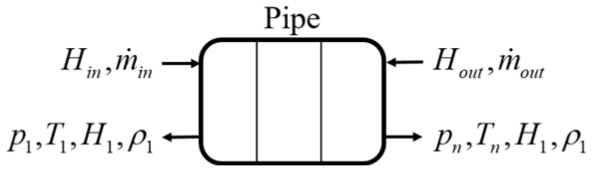
2.1. Pipe Model

The FESS is mainly composed of a pipe and regulating valve. Pipe bending, friction, heat transfer and other factors determine the main stable and dynamic characteristics of the system. The traditional lumped parameter model is difficult to reflect these characteristics, and a high-precision three-dimensional numerical simulation model has a large amount of calculation. Therefore, a quasi-one-dimensional pipe model is established in this paper.

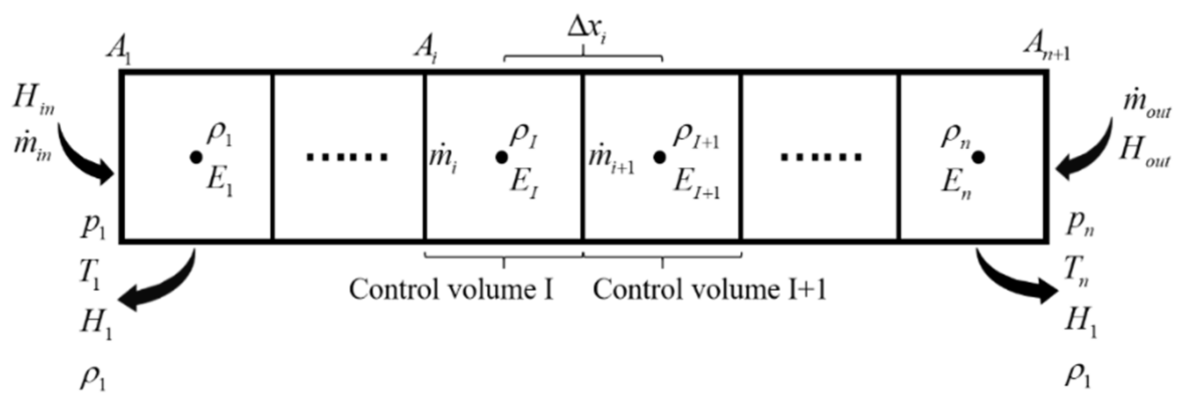
2.1.1. Quasi-One-Dimensional Flow in Pipe

Assumption:

• The fluid in control volume has uniform properties at each streamwise location.
• The axial heat transfer process and gravitational potential energy of the fluid are ignored.

According to the basic theory of fluid mechanics [15], the fluid in control volume satisfies the mass equation, energy equation and momentum equation as follows:

$$\frac{\partial }{\partial t}{\displaystyle {\int }_{\mathrm{CV}}\rho \mathrm{d}}V+{\displaystyle {\int }_{\mathrm{CS}}\rho \overrightarrow{u}\cdot \mathrm{d}\overrightarrow{A}}=0$$

(1)

$$\frac{\partial }{\partial t}{\displaystyle {\int }_{\mathrm{CV}}e\rho \mathrm{d}}V+{\displaystyle {\int }_{\mathrm{CS}}\left(e+\frac{p}{\rho }\right)\rho \overrightarrow{u}\cdot \mathrm{d}\overrightarrow{A}}=-\dot{Q}-\dot{W}$$

(2)

$$\frac{\partial }{\partial t}{\displaystyle {\int }_{\mathrm{CV}}\overrightarrow{u}\rho \mathrm{d}}V+{\displaystyle {\int }_{\mathrm{CS}}\overrightarrow{u}\rho \overrightarrow{u}\cdot \mathrm{d}\overrightarrow{A}}={\displaystyle \sum \overrightarrow{F}}$$

(3)

Based on the above assumptions, the grid with staggered spatial positions is introduced, as shown in Figure 1. Each grid in the pipe constitutes a control volume. The density and energy parameters of fluid are located in the center of the control volume, and the flow parameters of fluid are located at the boundary of the control volume.

According to the parameters of the center and boundary of the control volume, the corresponding derived parameters can be calculated [16] according to Equations (4)–(7). The derived parameters of the control volume’s center include fluid pressure, $p_I$, temperature, $T_I$, and total enthalpy $H_I$. The derived parameters of the control volume boundary include fluid velocity $u_i$. I represents the center of the control body, and i represents the front face of the I-th control volume.

$$u_i=\frac{{\dot{m}}_i}{0.5\left({\rho }_{I-1}+{\rho }_I\right)A_i}$$

(4)

$$T_I=\frac{\gamma -1}{R}\left(\frac{E_I}{m_I}-\frac{1}{8}{\left(u_i+u_{i+1}\right)}^2\right)$$

(5)

$$p_I={\rho }_{I}R{T}_I$$

(6)

$$H_I=\frac{E_I}{{\rho }_I{V}_I}+\frac{p_I}{{\rho }_I}$$

(7)

The quasi-one-dimensional flow model of pipe is established by the finite volume method. Equations (1)–(3) can be approximately equivalent to Equations (8)–(10) after discretization [16]. Equation (10) includes friction and local pressure losses. The unknown parameters of control volume are replaced by the mean value of the known parameters of adjacent control volumes.

$$\frac{\mathrm{d}{\rho }_I}{\mathrm{d}t}=\frac{1}{V_I}\left({\dot{m}}_i-{\dot{m}}_{i+1}\right)$$

(8)

$$\frac{\mathrm{d}{E}_I}{\mathrm{d}t}={\dot{m}}_i{H}_i-{\dot{m}}_{i+1}{H}_{i+1}-{\dot{Q}}_I$$

(9)

$$\frac{\mathrm{d}{\dot{m}}_i}{\mathrm{d}t}=\frac{{\dot{m}}_{I-1}\left|u_{I-1}\right|-{\dot{m}}_I\left|u_I\right|}{\Delta x_{i-1}}+\frac{A_i\left(p_{I-1}-p_I\right)}{\Delta x_{i-1}}-\frac{f{\rho }_i{u}_i\left|u_i\right|A_i}{2D}-\frac{K{\rho }_i{u}_i\left|u_i\right|A_i}{2\Delta x_{i-1}}$$

(10)

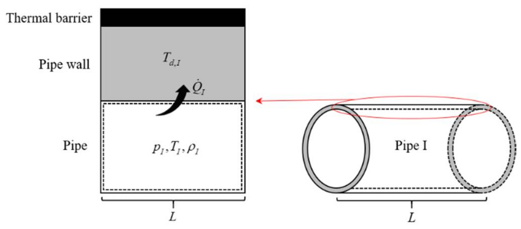
2.1.2. Heat Transfer Model of Pipe

The outside surface of the thin-walled pipe is wrapped with a thermal barrier and is segmented along the axial direction. Therefore, the radial heat conduction inside the metal pipe can be ignored. Only the heat convection process between the air flow and the metal pipe can be considered. The pipe is insulated from the external environment. The heat transfer process of the I-th control volume is shown in Figure 2.

Therefore, the pipe wall can be equivalent to an energy accumulator that changes its own energy by heat convection with air flow. The heat transfer rate between the pipe wall and air flow can be written as:

$${\dot{Q}}_I=h_f{A}_{d,I}\left(T_I-T_{d,I}\right)$$

(11)

The wall temperature change of the pipe is [11]:

$$\frac{\mathrm{d}{T}_{d,I}}{\mathrm{d}t}=\frac{{\dot{Q}}_I}{c_d{m}_{d,I}}$$

(12)

As shown in Figure 1, the parameters of the front face of the first control volume and the rear face of the last control volume (i.e., pipe boundary) are provided by the upstream and downstream components connected to the pipe, including mass flow and total enthalpy. Equations (8) and (9) are still applicable to the first and N-th control volumes. Since the mass flow at the boundary has been determined, the mass flow of the front face of the first control volume or the rear face of the last control volume do not need to be calculated by Equation (10). The external output parameters of the pipe are central parameters and derived parameters of the first and last control volumes. The interface parameters of the pipe model are shown in Figure 3.

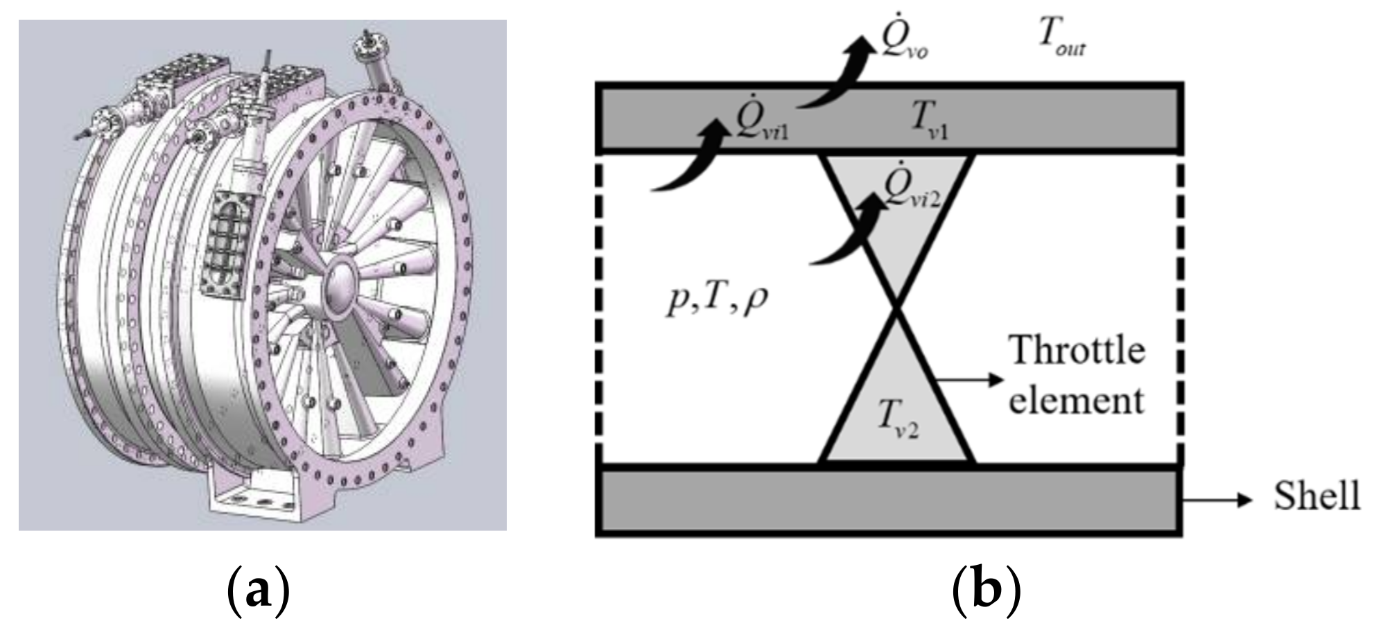
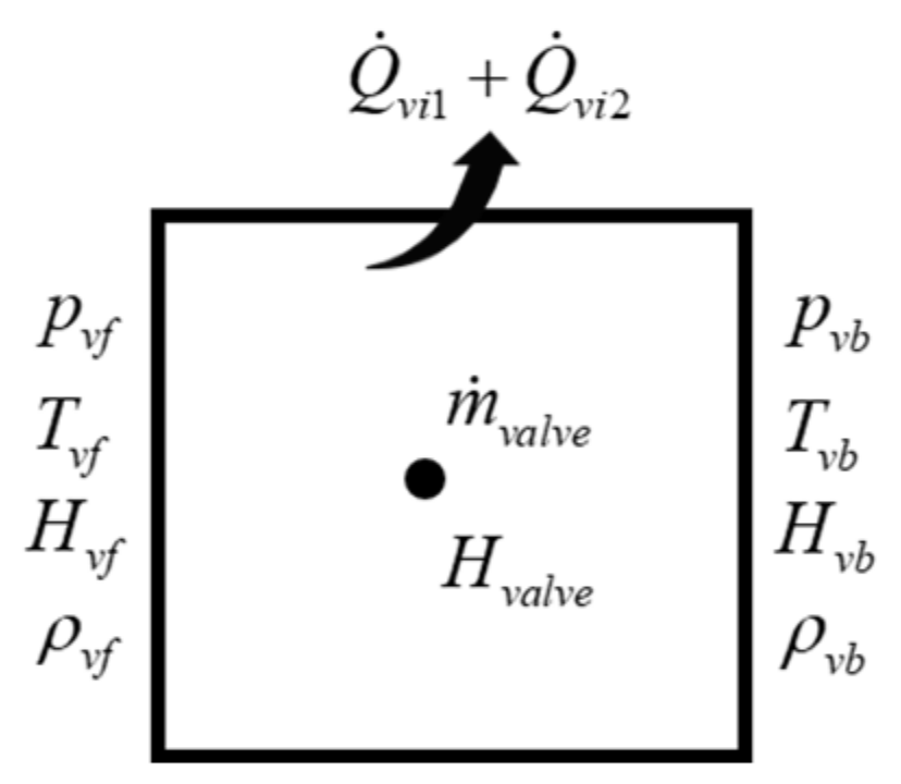
2.2. Regulating Valve Model

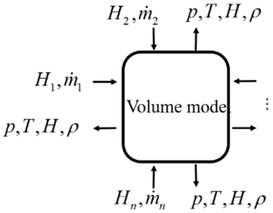
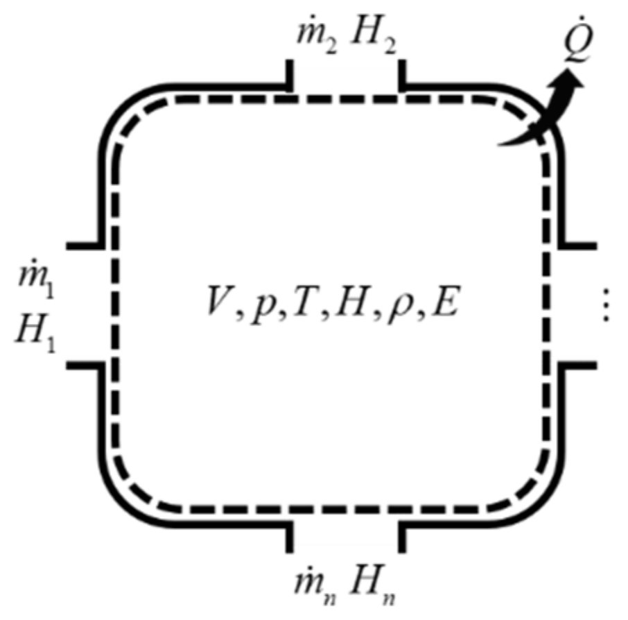
As a typical throttling element of the FESS, the regulating valve is mainly used for flow regulation. Its flow characteristic model can be established by the flow coefficient method [17,18].

$${\dot{m}}_{valve}=\phi A_v{p}_{vf}\sqrt{\frac{2}{R{T}_{vf}}}$$

(13)

where the flow coefficient is a function of the pressure ratio and flow area of the regulating valve, which can be obtained by fitting the experimental data [18]. The pressure ratio is as follows:

$$\pi =\frac{p_{vf}}{p_{vb}}$$

(14)

In previous studies, considering that the time of air flow through the regulating valve was very short, energy exchange between air flow and the regulating valve was ignored. However, for complex large diameter regulating valves such as disc regulating valves, the flow windows are small. The contact area between the valve body and air flow is large, and there are many valves installed between the pipes, resulting in a large energy loss of air flow through the valves. Therefore, based on the requirements of fine modeling, heat transfer process between the regulating valve and air flow or external environment must be considered. Due to the complex structure of the regulating valve, the fine heat transfer model of the regulating valve based on heat transfer mechanism is more complex. In this paper, the regulating valve shell is equivalent to a circular pipe participating in the heat transfer process of air flow and the external environment. The internal throttling element of the regulating valve is equivalent to an energy accumulator absorbing air energy. The structure of the regulating valve and its heat transfer process are shown in Figure 4.

${\dot{Q}}_{vi1}$ is the heat transfer rate between the shell and air flow. ${\dot{Q}}_{vi2}$ is the heat transfer rate between the throttling element and air flow. Their calculation process is consistent with Equation (11). $T_{v2}$ is the temperature of the throttling element, and its calculation process is consistent with Equation (12). The heat transfer process between the shell and the external environment shall be considered for the change of the shell temperature:

$$\frac{\mathrm{d}{T}_{v1}}{\mathrm{d}t}=\frac{{\dot{Q}}_{vi1}-h_f{A}_{vo}\left(T_{v1}-T_{out}\right)}{c_d{m}_{d,v}}$$

(15)

To build a regulating valve model that can be connected with the pipe model, a single control volume is established. It takes the inner wall surface of the regulating valve as a boundary, as shown in Figure 5. Unlike the pipe model, the central parameters of the control volume are the mass flow and total enthalpy, and the boundary of control volume is provided by the external components for pressure, temperature, total enthalpy, and density.

In Figure 5, the mass flow of the central section is calculated by Equation (13), and the total energy change rate of the air in the control volume can be written as:

$$\frac{\mathrm{d}{E}_v}{\mathrm{d}t}={\dot{m}}_{valve}\left(H_{vf}-H_{vb}\right)-{\dot{Q}}_{vi1}-{\dot{Q}}_{vi2}$$

(16)

The air density in the control volume is defined as ${\rho }_v=0.5\times \left({\rho }_{vf}+{\rho }_{vb}\right)$. The central flow rate of the control volume is computed by:

$$u_v=\frac{{\dot{m}}_{valve}}{{\rho }_v{A}_v}$$

(17)

The air flow temperature and total enthalpy in the control volume center are as follows:

$$T=\frac{\gamma -1}{R}\left(\frac{E_v}{{\rho }_v{V}_v}-\frac{1}{8}{u}_v{}^2\right)$$

(18)

$$H_{valve}=\frac{E_v}{{\rho }_v{V}_v}+RT$$

(19)

The total enthalpy and mass flow in the control volume center are transmitted to the external components as output parameters, and the interface parameters of the regulating valve model are shown in Figure 6.

2.3. Volume Model

The mixer and large cell of the FESS are mainly used for air flow mixing and pressure stabilization. There is no obvious axial movement of air flow. It is suitable to establish a volume model for such components. It is assumed that the volume has n ports, as shown in Figure 7. The boundaries of each port are the mass flow and total enthalpy. The internal parameters of volume include pressure, temperature, total enthalpy, and density.

According to the conservation of mass and energy, changes of air density and energy in the volume are as follows:

$$\frac{d\rho }{dt}=\frac{1}{V}{\displaystyle \sum _{i=1}^n{\dot{m}}_i}$$

(20)

$$\frac{\mathrm{d}E}{\mathrm{d}t}={\displaystyle \sum _{i=1}^n{\dot{m}}_i{H}_i}-\dot{Q}$$

(21)

For large volumes, the influence of air flow kinetic energy on total energy can be ignored. Referring to Equation (5), the air temperature and pressure in volume are as follows:

$$T=\frac{\gamma -1}{R}\frac{E}{\rho V}$$

(22)

$$p=\rho RT$$

(23)

Referring to Equation (7), the total enthalpy of air in volume is approximately as:

$$H=\frac{E}{\rho V}+\frac{p}{\rho }$$

(24)

The boundary parameters of the volume model are provided by external components, and the air flow parameters inside the volume are provided to the external components as output. The interface parameters of the volume model are shown in Figure 8.

2.4. Other Related Models

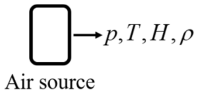
2.4.1. Air Source Model

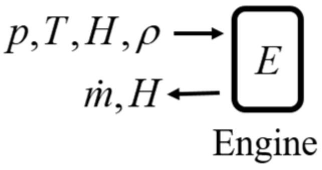
The air supply flow for the FESS comes from large compressors. The diameter of the air supply pipe is large and long. It can be regarded as a large pressure stabilizing volume and it can maintain a relatively constant temperature and pressure. At the same time, the inlet flow velocity is low, and the air kinetic energy can be ignored. Therefore, the air source model directly outputs the set pressure, temperature, total enthalpy, and density, as shown in Figure 9.

2.4.2. Engine Model

The FESS is divided into intake and exhaust subsystems, which provide intake and exhaust air environment for the engine, respectively. The engine inlet is connected with the intake subsystem through a flow pipe. The engine body and nozzle are connected with the exhaust subsystem. The intake and exhaust subsystems are connected through the engine. Therefore, when establishing the FESS simulation model, it is necessary to establish the engine flow characteristic model for the joint simulation of the FESS. The input of the engine model is temperature, pressure, total enthalpy, and density of air flow, and the output is engine intake flow. Considering that the engine is active suction and its inlet energy source is incoming flow, the output total enthalpy is consistent with the input total enthalpy, as shown in Figure 10.

Taking a typical turbofan engine as an example, a nonlinear mechanism model is established by a component-level modeling method. This engine model can be used to simulate the rapid change of airflow during the acceleration and deceleration of the aircraft engine, which can more realistically reflect the impact of the aircraft engine on the FESS. For the engine model, all component characteristic maps and relevant data are acquired from a commercial software called GSP. Many studies have been carried out on this model [19,20], and the model has high reliability and can be directly used in this paper.

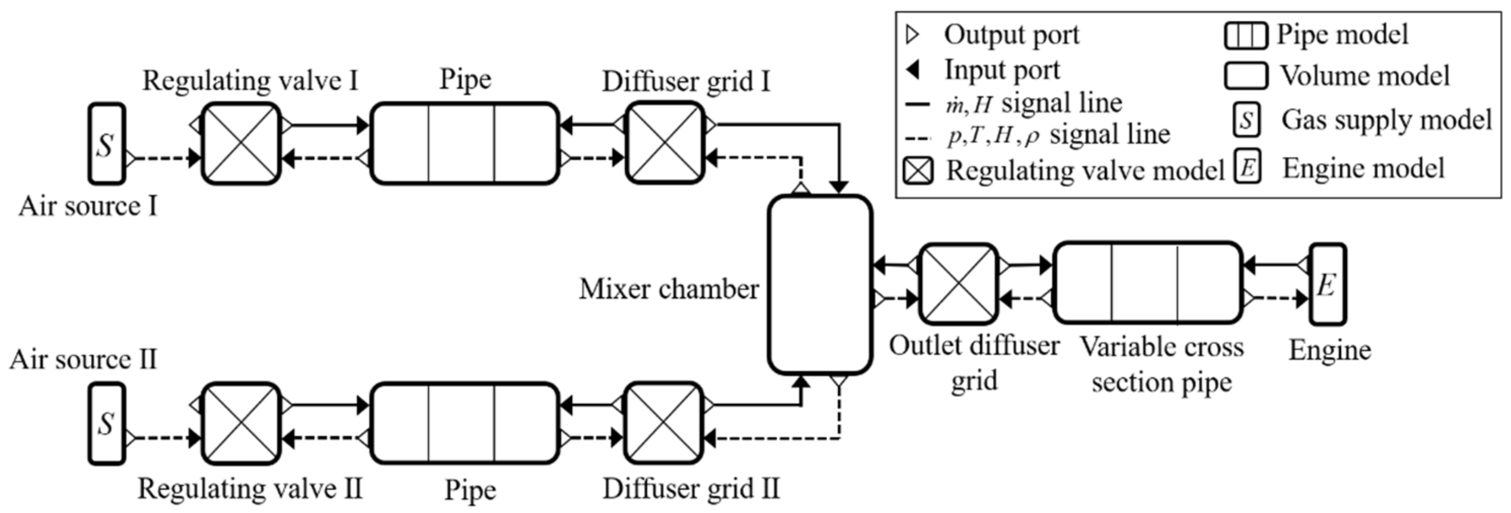
3. Simulation Model of the FESS

Since a single air source can only provide airflow with a fixed temperature and pressure, two different air sources are used for mixing to obtain airflow with different temperatures and pressures, which will be provided to the engine. The structural diagram of the FESS, which is mainly composed of pipes, volumes and throttling elements, is shown in Figure 11. The two air supply flows are adjusted through regulating valve I and regulating valve II. After mixing in the mixer, the air flows into test engine through a variable cross section pipe. Based on the above component models, the numerical simulation model of the FESS can be constructed.

In addition, the diffuser grids of the mixer are throttling elements, which can be considered as regulating valves with a constant throttling area. They can then be replaced by a regulating valve model, and their flow coefficients can be obtained through three-dimensional flow field simulation calculation. The mixer has an effect of air mixing, which can be replaced by the volume model. Other pipes are modeled by the pipe model. According to the actual structure of the FESS, the system level simulation model is constructed, and the connection between each module is shown in Figure 12.

In Figure 12, the input and output ports between the modules are connected in sequence. The modeling method based on component model improves system level modeling efficiency and enhances scalability of the simulation model. The configuration parameters of each module in the simulation model are set according to the actual physical structure of the FESS. The pipe model divides the grids according to the positions of the variable section, elbow, and local obstacles. The diffuser grid is located inside the pipe flow field. The regulating valve model can be used to calculate the mass flow through the diffuser grid, but the shell heat transfer calculation should be closed in the regulating valve model. Only the accumulator heat transfer calculation is retained. In addition, in order to ensure the normal operation of the model, the process simulated by the model should be consistent with the actual technological process. Firstly, open the regulating valve to make the system establish a certain pressure, temperature, and flow environment. Then, start the engine and carry out subsequent simulations.

4. Model Simulation and Verification

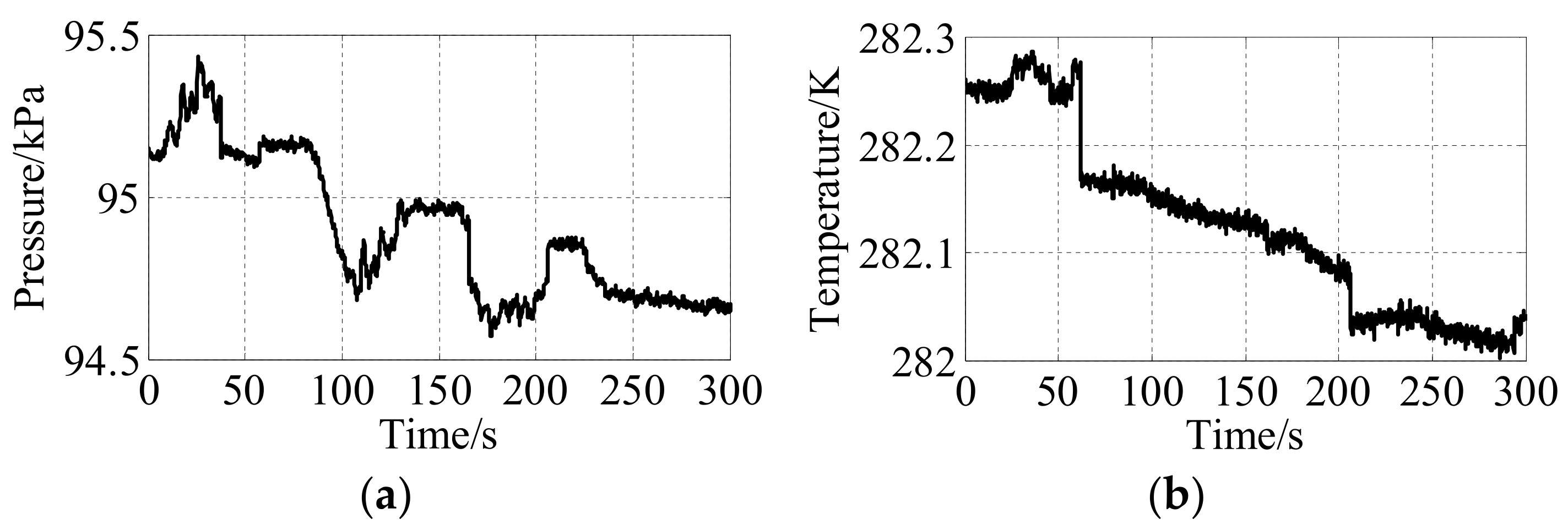
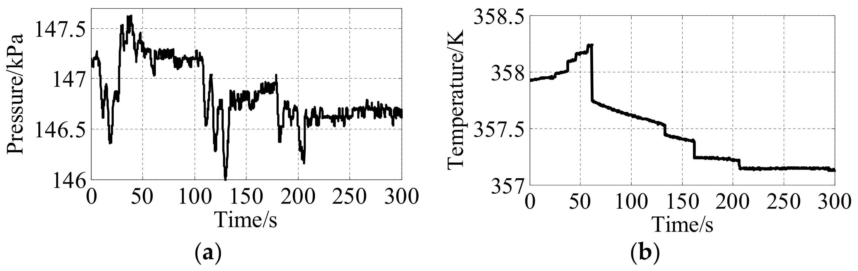
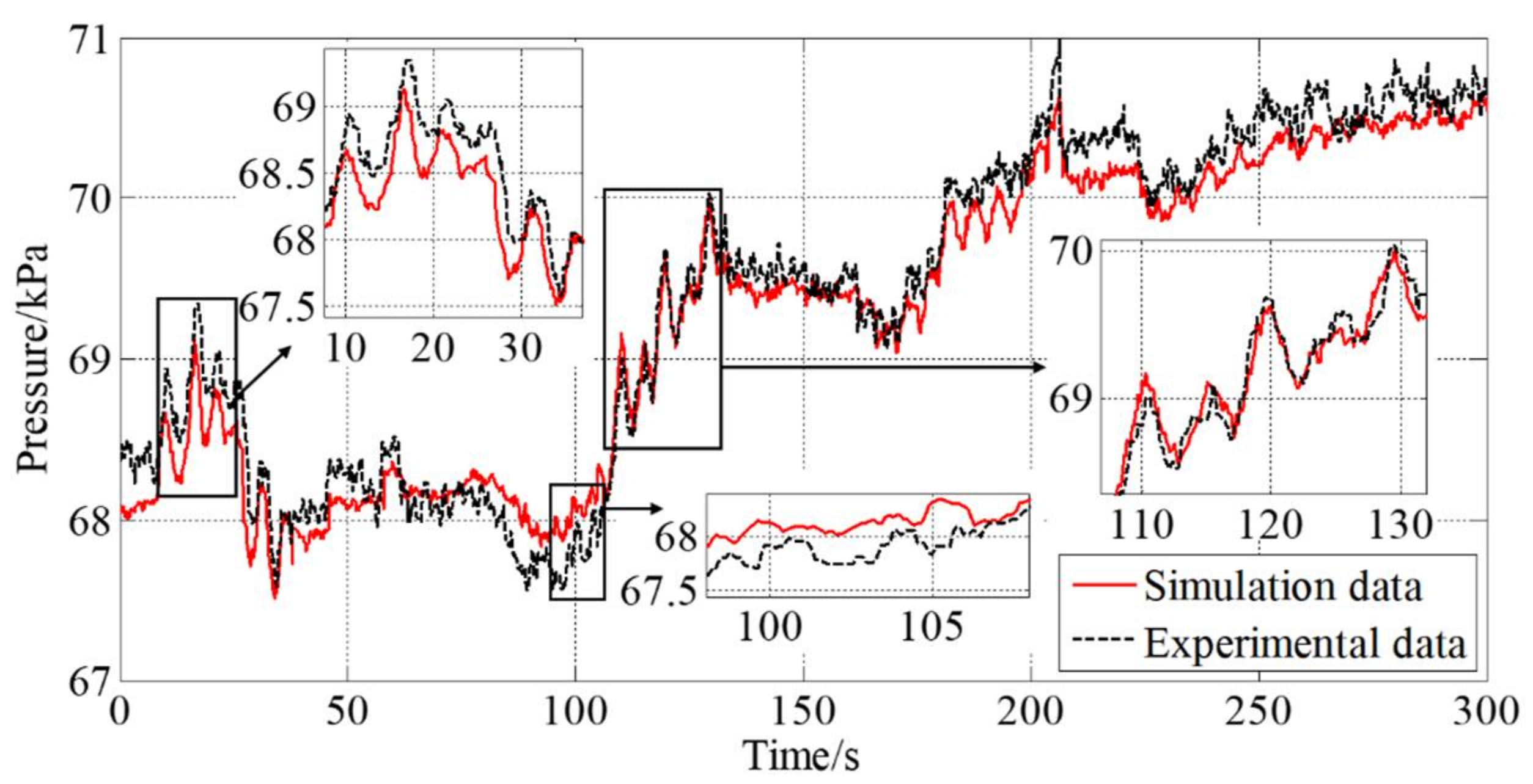
4.1. Model Verification

To further verify the model’s accuracy, the simulation under typical working conditions is carried out and compared with experimental data. It is worth noting that the parameters, such as inlet pressure and temperature, are closed-loop control parameters during the flight environment simulation test at AGTF.

According to the experimental data, the simulation conditions required for model simulation are extracted, including pressure and temperature of the two air sources, opening change of the two regulating valves, and outlet pressure and temperature of the variable section pipeline (ignoring the engine model), as shown in Figure 13, Figure 14, Figure 15 and Figure 16. This is the air flow mixing process of the FESS. Under the given inlet and outlet boundary conditions, the required air flow is provided by adjusting the opening of the two regulating valves. Boundary conditions are set in the FESS model (as shown in Figure 13, Figure 14 and Figure 16), the opening of the regulating valves is adjusted (as shown in Figure 15) to carry out the simulation.

The comparison results between the model calculation data and the experimental data are shown in Figure 17. The model simulation results are basically consistent with the experimental data. The outlet flow of the variable cross section pipe is calculated by the air flow parameters measured by the temperature sensor 2 and pressure sensor 2 on the pipe, as shown in Figure 11. The sensors used to calculate the flow have high acquisition frequency and a large amount of data, while the data acquisition frequency of temperature sensor 3, pressure sensor 1, and pressure sensor 3 are low, as shown in

Table 1. Accuracy and sampling rate of sensors.

Sensors	Accuracy	Acquisition Frequency
pressure sensor 1	$\pm$0.05 kPa	20 Hz
pressure sensor 2	$\pm$0.05 kPa	50 Hz
pressure sensor 3	$\pm$0.05 kPa	20 Hz
temperature sensor 2	$\pm$0.1 K	50 Hz
temperature sensor 3	$\pm$0.1 K	20 Hz

. Therefore, there is a certain deviation between the test data and the simulation data. In addition, the flow coefficient of the regulating valve is fitted according to some experimental data and three-dimensional flow field simulation data. There is a certain deviation from the actual value under some opening, which will also lead to a certain steady-state error. Figure 18 shows the flow error diagram, in which the maximum flow deviation is less than 8 kg/s and the maximum flow relative error is 4.4%.

In order to further verify the confidence of the model, the pressure change of cross Section 1 in Figure 11 is selected for comparison. As shown in Figure 19, the pressure change shows good consistency between 110 and 130 s and can maintain a consistent dynamic change trend. In Figure 20, it can be seen that the maximum deviation of pressure is less than 0.7 kPa and the maximum relative error is 0.9%. The model simulation accuracy can meet the engineering requirements of control algorithm research and verification. For the lumped parameter model, the maximum deviation and relative error of pressure are 2 kPa and 3.1%, respectively [11]. The advantages of the quasi-one-dimensional flow model are further verified.

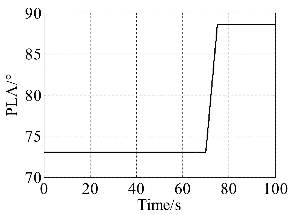
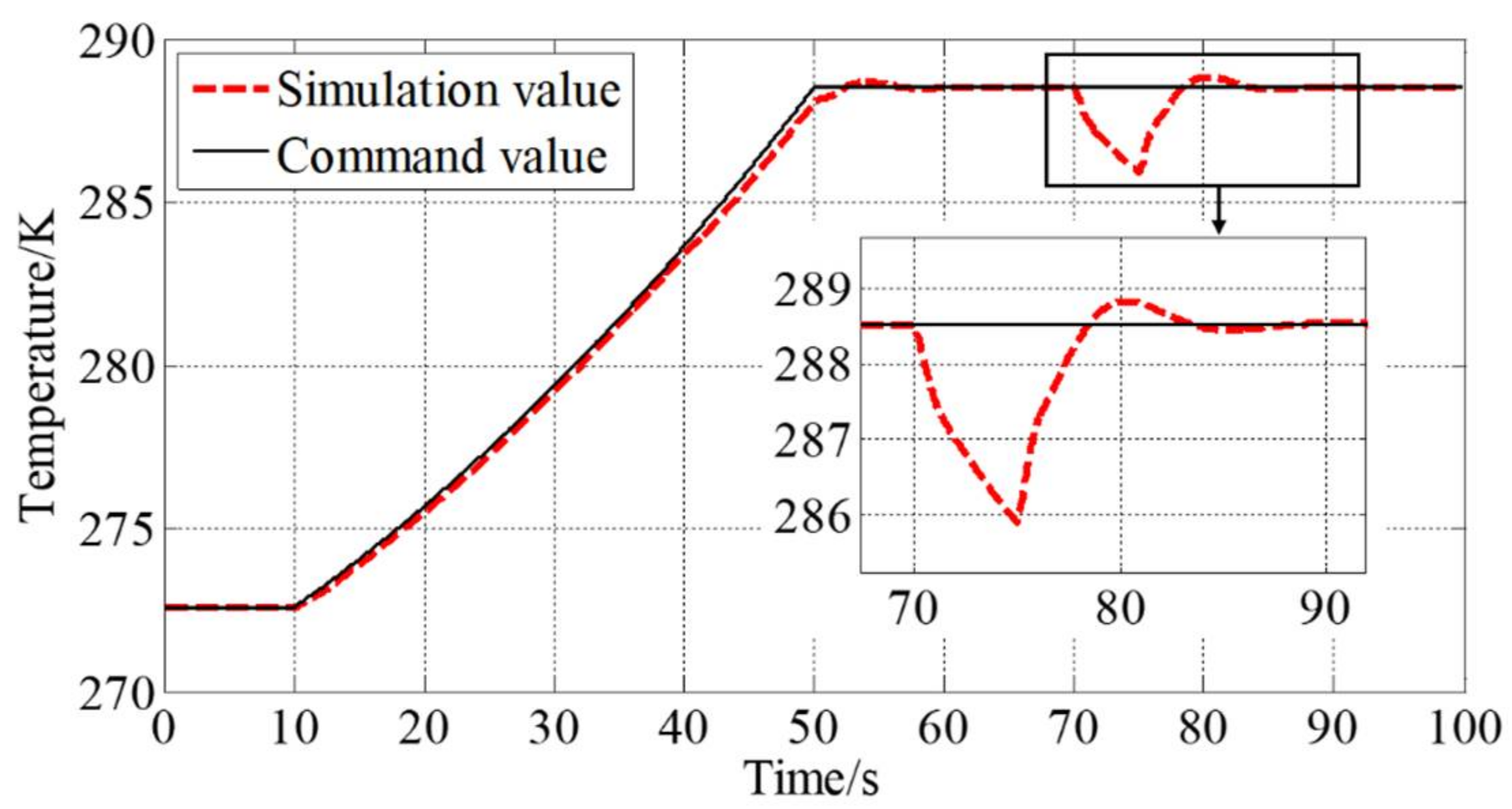
4.2. Closed-Loop Control Simulation of Intake Air Temperature and Pressure

Verifying the effectiveness of the control algorithm is one of the main uses of the FESS model. Therefore, the simulation of the closed-loop control system is carried out to test whether the system level model has the ability to verify the performance of the controller. In the simulation process, air supply conditions are set as follows: the pressure of air source I is 118 kPaand the temperature is 255 K; the pressure of air source II is 135 kPa and the temperature is 305 K. The flight altitude of the engine is set to remain unchanged at 3.4 km, and the Mach number increases from 0.35 to 0.65 in 40 s. This process simulates the working process of engine acceleration at a constant altitude, as shown in Figure 21. The throttle lever angle increases from 73 degrees to 88.6 degrees in 5 s. This process simulates the engine thrust transient, as shown in Figure 22.

In the whole simulation process, according to the flight altitude and Mach number conditions, the pressure and temperature of the outlet air flow can be calculated by using the engine flight altitude and speed characteristics. Regulating valve I and regulating valve II are used to control the temperature and pressure at the outlet of the variable section pipe. PI controllers are designed for regulating valve I and regulating valve II. The FESS model is used for simulation test and verification. The control effects of air flow temperature and pressure at the outlet of the variable section pipe are shown in Figure 23 and Figure 24. The outlet mass flow is shown in Figure 25. It can be seen that, in the engine acceleration at constant altitude stage, the air flow pressure and temperature can track the command change, and there is a small fluctuation at the end of regulation. Although the throttle lever angle of the engine remains unchanged, the outlet mass flow increases by 17 kg/s due to the change of air temperature and pressure. The change of flow will further affect the air flow parameters, indicating that there is a coupling relationship between the engine and the FESS. In the transient stage of engine thrust, the air flow increases by 56.8 kg/s due to the increase of throttle lever angle. For the FESS, the engine can be regarded as a disturbance. Due to the coupling of control loops of the two control valves, the pressure fluctuation exceeds 1 kPa and the temperature fluctuation exceeds 2.6 K.

The opening change of the regulating valve is shown in Figure 26. To ensure that the outlet air flow temperature increases, the opening of regulating valve II controlling high-temperature air flow increases. To suppress the increase of outlet pressure caused by the increase of flow, the opening of regulating valve I decreases. Because the PI controller cannot effectively solve the coupling influence of the outlet air flow temperature and pressure, the control effect is poor in the process of large disturbances such as transient thrust. It is necessary to adopt decoupling or multivariable control methods to realize high-precision control of the outlet air flow pressure and temperature.

In addition to verifying the control algorithms, the quasi-one-dimensional flow model of the FESS can also be used for controller design. In fact, factors such as one-dimensional flow, friction, local heat transfer, and local pressure loss cause the FESS model to have time-delay characteristics, strong nonlinearity, and large uncertainty. Therefore, when designing the controller, a reasonable and accurate linear or nonlinear model can be obtained based on the FESS model. Through the simulation and analysis of the FESS model, the complex system characteristics of the FESS can be studied, and then an effective control algorithm can be designed to deal with the time-delay, nonlinearity, and uncertainty of the FESS.

5. Conclusions

In order to improve the accuracy of the FESS model, a modeling method based on quasi-one-dimensional flow was presented in this paper. The simulation models of the FESS are established. Through the simulation verification of experimental data and closed-loop system testing, the following conclusions are drawn.

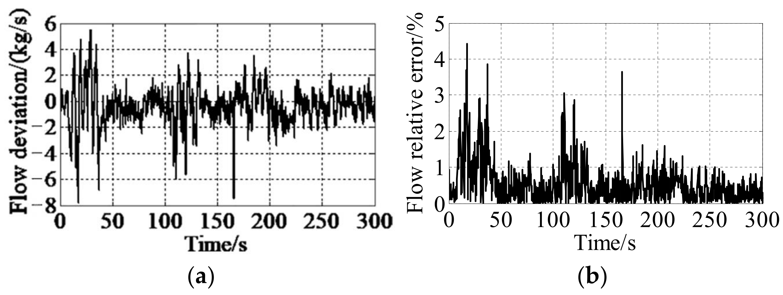
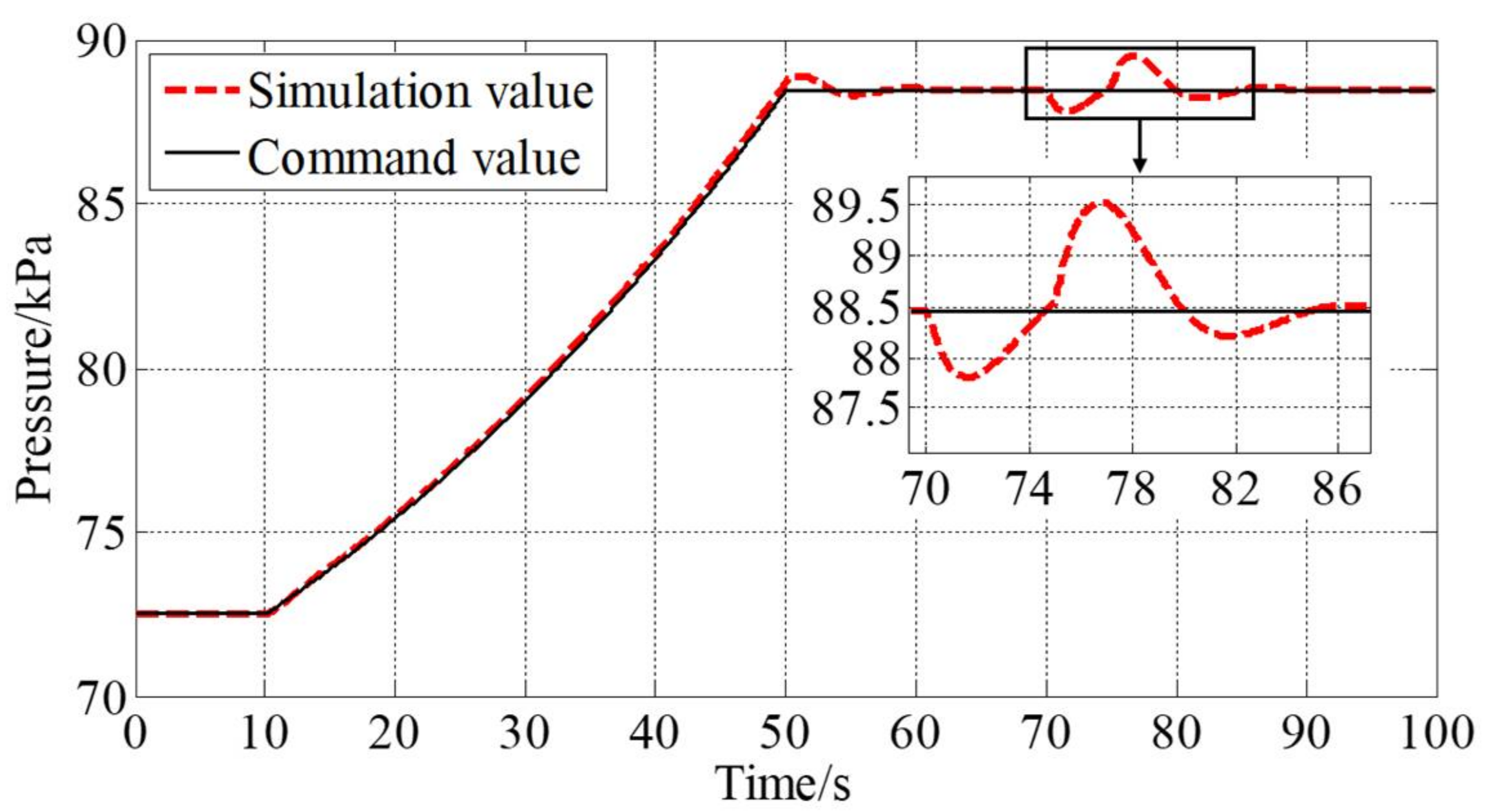
• The simulation results under typical working conditions are compared with the experimental data to verify that the model has high confidence, in which the relative error of mass flow is no more than 4.4%, and the relative error of pressure at the specified cross section is no more than 0.9%. The model can meet the actual needs in engineering.
• The model has the ability to verify and test the system control algorithm and can support the development and verification of advanced technology of the FESS.
• The model is affected by the flow coefficient of the regulating valve and other parameters. With the accumulation of a large number of experimental data and the calculation of high-precision three-dimensional simulation data, the accuracy of the model can be further improved.

References

1. Montgomery, P.A.; Burdette, R.; Krupp, B. A Real-Time Turbine Engine Facility Model and Simulation for Test Operations Modernization and Integration. In Proceedings of the ASME Turbo Expo 2000: Power for Land Sea, and Air, Munich, Germany, 8–11 May 2000. [Google Scholar] [CrossRef]
2. Montgomery, P.A.; Burdette, R.; Wilhite, L.; Salita, S. Modernization of a Turbine Engine Test Facility Utilizing a Real-Time Facility Model and Simulation. In Proceedings of the ASME Turbo Expo 2001: Power for Land Sea, and Air, New Orleans, LA, USA, 4–7 June 2001. [Google Scholar] [CrossRef]
3. Davis, M.; Montgomery, P. A Flight Simulation Vision for Aeropropulsion Altitude Ground Test Facilities. In Proceedings of the ASME Turbo Expo 2002: Power for Land Sea, and Air, Amsterdam, The Netherlands, 3–6 June 2002. [Google Scholar] [CrossRef]
4. Sheeley, J.M.; Sells, D.A.; Bates, L.B. Experiences with Coupling Facility Control Systems with Control Volume Facility Models. In Proceedings of the 42ndAIAA Aerospace Sciences Meeting and Exhibit, Reno, NE, USA, 5–8 January 2004. [Google Scholar] [CrossRef]
5. Butler, K.; Milhoan, A. Upgrades to the Aerodynamic and Propulsion Test Unit Heated Fuel System. In Proceedings of the 19th AIAA International Space Planes and Hypersonic Systems and Technologies Conference, Atlanta, GA, USA, 16–20 June 2014. [Google Scholar] [CrossRef]
6. Boraira, M.; Van Every, D. Design and Commissioning of a Multivariable Control System for A Gas Turbine Engine Test Facility. In Proceedings of the 25th AIAA Aerodynamic Measurement Technology and Ground Testing Conference, San Francisco, CA, USA, 5–8 June 2006. [Google Scholar] [CrossRef]
7. Schmidt, K.J.; Merten, R.; Menrath, M.; Braig, W. Adaption of The Stuttgart University Altitude Test Facility for BR700 Core Demonstrator Engine Tests. In Proceedings of the ASME International Gas Turbine & Aeroengine Congress & Exhibition: The American Society of Mechanical Engineers, Stockholm, Sweden, 2–5 June 1998. [Google Scholar] [CrossRef] [Green Version]
8. Bierkamp, J.; Köcke, S.; Staudacher, S.; Fiola, R. Influence of ATF Dynamics and Controls on Jet Engine Performance. In Proceedings of the ASME Turbo Expo 2007: Power for Land Sea, and Air, Montreal, QC, Canada, 14–17 May 2007. [Google Scholar] [CrossRef]
9. Weisser, M.; Bolk, S.; Staudacher, S. Hard-in-the-Loop-Simulation of a Feedforward Multivariable Controller for the Altitude Test Facility at the University of Stuttgart. 2013. Available online: https://www.dglr.de/publikationen/2013/301179 (accessed on 9 February 2022).
10. Pei, X.T.; Zhang, S.; Dan, Z.H.; Zhu, M.Y.; Qian, Q.M.; Wang, X. Study on Digital Modeling and Simulation of Altitude Test Facility Flight Environment Simulation System. J. Propul. Technol. 2019, 40, 1144–1152. [Google Scholar] [CrossRef]
11. Zhu, M.Y.; Wang, X.; Pei, X.T.; Zhang, S.; Dan, Z.H.; Miao, K.Q.; Liu, J.S.; Jiang, Z. Multi-Volume Fluid-Solid Heat Transfer Modeling for Flight Environment Simulation System. J. Propul. Technol. 2020, 41, 2848–2859. [Google Scholar] [CrossRef]
12. Zhu, M.Y.; Wang, X.; Zhang, S.; Dan, Z.H.; Pei, X.T.; Miao, K.Q.; Jiang, Z. PI Gain Scheduling Control for Flight Environment Simulation System of Altitude Ground Test Facilities Based on LMI Pole Assignment. J. Propul. Technol. 2019, 40, 2587–2597. [Google Scholar] [CrossRef]
13. Zhu, M.Y.; Wang, X.; Pei, X.T.; Zhang, S.; Dan, Z.H.; Liu, J.S.; Miao, K.Q.; Jiang, Z. Temperature Delay Uncertainty μ Synthesis for Flight Environment Simulation System of Altitude Ground Test Facilities. J. Propul. Technol. 2020, 41, 1861–1870. [Google Scholar] [CrossRef]
14. Dan, Z.H.; Zhang, S.; Bai, K.Q.; Qian, Q.M.; Pei, X.T.; Wang, X. Air Intake Environment Simulation of Altitude Test Facility Control Based on Extended State Observer. J. Propul. Technol. 2021, 42, 2119–2128. [Google Scholar] [CrossRef]
15. Wang, X.Y. Fundamentals of Aerodynamics; Northwestern Polytechnical University Press: Xi’an, China, 2006; pp. 56–69. ISBN 7-5612-2142-8. [Google Scholar]
16. Boylston, B.M. Quasi-One-Dimensional Flow for Use in Real-Time Facility Simulations. Master’s Thesis, University of Tennessee, Knoxville, TN, USA, 2011. Available online: https://trace.tennessee.edu/utk_gradthes/1058 (accessed on 9 February 2022).
17. Pei, X.T.; Zhu, M.Y.; Zhang, S.; Dan, Z.H.; Wang, X.; Wang, X. An Iterative Method of Empirical Formula for the Calculation of Special Valve Flow Characteristics. Gas Turb. Exp. Res. 2016, 29, 35–39. Available online: https://kns.cnki.net/kcms/detail/detail.aspx?FileName=RQWL201605009&DbName=CJFQ2016 (accessed on 9 February 2022).
18. Zhu, M.Y.; Pei, X.T.; Zhang, S.; Dan, Z.H.; Wang, X.; Wang, X. A Modified Algorithm for Flow Characteristics of Disc Type Special Control Valve. Gas Turb. Exp. Res. 2016, 29, 40–45. Available online: https://kns.cnki.net/kcms/detail/detail.aspx?FileName=RQWL201605010&DbName=CJFQ2016 (accessed on 9 February 2022).
19. Yang, S.B.; Wang, X.; Wang, H.N.; Li, Y.G. Sliding Mode Control with System Constraints for Aircraft Engines. ISA Trans. 2019, 98, 1–10. [Google Scholar] [CrossRef] [PubMed]
20. Yang, S.B.; Wang, X.; Yang, B. Adaptive Sliding Mode Control for Limit Protection of Aircraft Engines. Chin. J. Aeronaut. 2018, 31, 1480–1488. [Google Scholar] [CrossRef]
Figure 1. Schematic diagram of axial grid division of pipe.
Processes 10 00377 g001
Figure 2. Schematic diagram of heat transfer process.
Processes 10 00377 g002
Figure 3. Interface parameters of pipe model.
Processes 10 00377 g003
Figure 4. Regulating valve and its heat transfer process. (a) Regulating valve; (b) Heat transfer process.
Processes 10 00377 g004
Figure 5. Schematic diagram of regulating valve control volume.
Processes 10 00377 g005
Figure 6. Interface parameters of regulating valve model.
Processes 10 00377 g006
Figure 7. Schematic diagram of volume model.
Processes 10 00377 g007
Figure 8. Interface parameters of volume model.
Processes 10 00377 g008
Figure 9. Interface parameters of air source.
Processes 10 00377 g009
Figure 10. Interface parameters of engine.
Processes 10 00377 g010
Figure 11. Schematic diagram of Flight Environment Simulation System.
Processes 10 00377 g011
Figure 12. Module connection diagram in the simulation model.
Processes 10 00377 g012
Figure 13. Inlet conditions of air source I. (a) Pressure conditions of air source I; (b) Temperature conditions of air source I.
Processes 10 00377 g013
Figure 14. Inlet conditions of air source II. (a) Pressure conditions of air source II; (b) Temperature conditions of air source II.
Processes 10 00377 g014
Figure 15. Opening change process of two regulating valves.
Processes 10 00377 g015
Figure 16. Outlet conditions of variable cross section pipe. (a) Pressure outlet conditions; (b) Temperature outlet conditions.
Processes 10 00377 g016
Figure 17. Comparison of outlet flow of variable cross section pipe.
Processes 10 00377 g017
Figure 18. Mass flow error. (a) Flow deviation; (b) Flow relative error.
Processes 10 00377 g018
Figure 19. Comparison of pressure changes in cross Section 1.
Processes 10 00377 g019
Figure 20. Pressure error. (a) Pressure deviation; (b) Pressure relative error.
Processes 10 00377 g020
Figure 21. Altitude and Mach number test conditions. (a) Altitude test conditions; (b) Mach number test conditions.
Processes 10 00377 g021
Figure 22. Throttle rod angle.
Processes 10 00377 g022
Figure 23. Pressure change of outlet air flow.
Processes 10 00377 g023
Figure 24. Temperature change of outlet air flow.
Processes 10 00377 g024
Figure 25. Mass flow change of outlet air flow.
Processes 10 00377 g025
Figure 26. Opening of regulating valves.
Processes 10 00377 g026