Article

A Joint Stacked Autoencoder Approach with Silhouette Information for Industrial Fault Detection

1
State Key Laboratory of Synthetical Automation for Process Industries, Northeastern University, Shenyang 110819, China
2
State Key Laboratory of ASIC and System, School of Microelectronics, Fudan University, Shanghai 201203, China
3
Academy of Engineering and Technology, Shanghai Engineering Research Center of UPMCM, Fudan University, Shanghai 200433, China
*
Author to whom correspondence should be addressed.
These authors contributed equally to this work.
Processes 2022, 10(11), 2408; https://doi.org/10.3390/pr10112408
Submission received: 18 October 2022 / Revised: 9 November 2022 / Accepted: 10 November 2022 / Published: 15 November 2022
(This article belongs to the Section Chemical Processes and Systems)

Abstract

:
Due to the growing complexity of industrial processes, it is no longer adequate to perform precise fault detection based solely on the global information of process data. In this study, a silhouette stacked autoencoder (SiSAE) model is constructed for process data by considering both global/local information and silhouette information to depict the link between local/cross-local. Three components comprise the SiSAE model: hierarchical clustering, silhouette loss, and the joint stacked autoencoder (SAE). Hierarchical clustering is used to partition raw data into many blocks, which clarifies the information’s characteristics. To account for silhouette information between data, a silhouette loss function is constructed by raising the inner block’s data distance and decreasing the distance of the cross-center block. Each data block has a properly sized SAE model and is jointly trained via silhouette loss to extract features from all available data. Using the Tennessee Eastman (TE) benchmark and semiconductor industrial process data, the proposed method is validated. Comparative tests on the TE benchmark indicate that the average rate of fault identification increases from 75.8% to 83%, while the average rate of false detection drops from 4.6% to 3.9%.

1. Introduction

In order to assure the dependability and safety of industrial manufacturing, fault detection has attracted growing attention [1,2,3]. Numerous types of industrial process measurement data have been collected as a result of the rapid development of computing technologies and the gradual integration of industrial processes. Thus, significant progress has been made in data-driven industrial fault detection techniques, of which multivariate statistical process monitoring (MSPM) is an important branch [4,5,6,7]. The central concept of MSPM is to project high-dimensional process data onto a low-dimensional set of latent variables and then to develop statistical indicators for fault detection [8]. The principal component analysis (PCA) and independent component analysis (ICA) are representative approaches in MSPM that are only suitable for feature extraction with variables that have a linear relationship [9]. Methods such as the kernel PCA and kernel ICA are used to extract more precise features for industrial defect detection in order to solve the problem [10]. However, it is difficult to recreate the input in complicated industrial processes using features collected from previous MSPM approaches, rendering the values of squared prediction error unreliable for defect detection [4].
Deep learning approaches are more effective for extracting high-order feature information and reconstructing data than MSPM [11,12]. An intelligent fault diagnosis method combined with the advantages of deep learning was designed to solve the speed fluctuation problem [13]. A novel transfer learning method combined with an adversarial network was proposed to deal with the data shift problem and improve the detection accuracy [14]. Both demonstrate the strong feature extraction capability of the deep learning approach. The autoencoder (AE), as another deep learning technique, accomplishes automated dimensionality reduction. It has a powerful ability to learn the nonlinear characteristics of process data and can create deeper models by stacking layers and using a more generalized model with more data [15,16]. On the basis of the AE, the variable-wise weighted stacked auto-encoder was proposed. This extracts globally significant variable output-related features to increase the detection performance [17]. It has been proposed that recurrent neural networks and the variational autoencoder could be combined to manage dynamic processes [18]. However, these methods mainly focus on the global information in the data and rarely take local information into account, which may hinder the defect detection performance.
The local information in the data is crucial for the detection accuracy and its importance has been demonstrated [19,20]. To construct the local model, the variable subset partition approach is used to divide variables into linear and nonlinear subsets [21]. In addition, a novel model is created that may segregate the data into static and dynamic aspects for distinct modeling [22]. Both divide variables into two primary components and construct a more accurate model than when only global information is used.
In order to collect more local information, the understanding of the mechanism and mutual information are also employed to properly partition global variables and extract local information in order to take local information into account [23,24]. However, it is difficult to analyze the blocking strategies of mechanistic knowledge from a global perspective due to the link between the input and output cross-units. Methods of mutual information necessitate a continuous threshold that is challenging to select when describing the actual clustering number and data features. In addition, cross-local information is rarely considered. A distributed-ensemble stacked autoencoder (DE-SAE) model is proposed. This used the cross-unit information by the joint local feature [25]. Self-attention is used to integrate aspects from each block in order to examine cross-block information [26]. Both consider cross-block information using joint features. However, these methods employ separate modeling for pretraining and are incapable of achieving joint training to depict the entire process, so they do not consider local and cross-local information in their entirety.
In this study, a silhouette stacked autoencoder (SiSAE) model was developed by incorporating both global/local information and the local silhouette information of the process data. The model consists of three parts: hierarchical clustering, silhouette loss, and joint SAE. By going through the process of hierarchical clustering, each partition of the data has the characteristics of high cohesiveness and low coupling, which facilitates the effective acquisition of local and cross-local information. For more effective information, a novel loss function termed silhouette loss is proposed. This raises the inner-block distance of each block and decreases the cross-block distance of each block. Lastly, each data block has an SAE model of the proper size and is jointly trained using silhouette loss to accurately reflect the entire process. To evaluate the superiority and viability of the developed approach, the Tennessee Eastman (TE) benchmark process and a semiconductor industrial process were carried out, and an outstanding fault detection performance was obtained.
The remainder of the article’s is structured as follows. In Section 2, pertinent technologies, including agglomerative hierarchical clustering, SAE, kernel density estimation, and the moving average approach are described. The proposed SiSAE model and silhouette loss are clarified in Section 3. Two industrial processes are used to demonstrate the superiority and viability of the suggested method in Section 4. In Section 5, the conclusions are presented.

2. Preliminaries

2.1. Agglomerative Hierarchical Clustering

Hierarchical clustering is an unsupervised learning approach that is used for discovering natural groupings in the feature space of input data. It splits the data set into a number of distinct clusters or blocks based on a predetermined criterion, resulting in a tree-like clustering structure. Typically, the Euclidean distance is employed to determine the similarity between data points within each category. Smaller distances indicate greater similarity and the likelihood of belonging to a category. In n-dimensional Euclidean space, the euclidean distance between points x ( x i 1 , x i 2 , . . . , x i n ) and y ( y j 1 , y j 2 , . . . , y j n ) is calculated as follows:
d i j = k = 1 n ( x i k y j k ) 2 .
Agglomerative hierarchical clustering is a bottom-up hierarchical clustering method that initially treats each original data set as a single cluster before aggregating smaller clusters into larger clusters until the final criterion is met. In addition, there are four traditional ways to estimate the distance between clusters: the single-linkage method, the complete-linkage method, the average-linkage method, and the ward-linkage method. The ward-linkage approach, which minimizes the variance of the merging clusters, was applied to the articles since it is the most appropriate for quantitative variables. The Ward-linkage approach demonstrates that the distance between two clusters, A and B, is proportional to the increase in the sum of squares when they are merged, and it has the following expressions:
( A , B ) = n A n B n A + n B m A m B 2
where m j is the center of cluster j ( A , B ) , and n j is the number of points included within it. The cost of combining the clusters A and B is denoted by △. With clustering, the sum of squares begins at zero and gradually increases as clusters merge.

2.2. Stacked Autoencoder

Autoencoders (AEs) are unsupervised neural networks with one hidden layer that is composed of an encoder and a decoder and uses a back-propagation method to match the output value to the input value as precisely as possible. The input is first compressed into a possible spatial representation, and then the output is reconstructed using this representation. The complete network is always shaped like an hourglass with the input and output layers being larger than the hidden levels. Figure 1 depicts the fundamental framework of an AE model.
Assume that the input of the AE is x = [ x 1 , x 2 , . . . , x n ] T R n , where n is the dimensions of the input. The hidden layer h = [ h 1 , h 2 , . . . , h m ] T R m in the encoder is obtained from the input layer x by means of a mapping function f as
h = f ( x ) = σ ( W x + b )
where m is the dimensions of the hidden vector; W is a m n weight matrix; and b R m is a bias vector. σ is a nonlinear activation function, such as the relu function or tanh function.
The function f ¯ maps the hidden vector h to the output layer x R n in the decoder, as follows:
x = f ¯ ( h ) = σ ¯ ( W h + b )
where W is a n m weight matrix and b R n is a bias vector. The σ ¯ is the activation function. The AE is trained to acquire the model parameters by reducing the mean squared error. The error loss function is given by Equation (5), and the gradient descent approach can be used to update the parameters.
l o s s ( x , x ) = 1 2 n k = 1 n x k x k 2
where x k represents the k t h input’s data, and x k is the k t h output’s data. x k x k are referred to as reconstruction errors.
The stacked AE is a deep network model that is formed by layer-by-layer stacking of the input and hidden layers of AEs. Figure 2 depicts the architecture of the SAE. The SAE training procedure consists of two phases: layer-by-layer pre-training and fine-tuning. In the initial stages, each unit of the SAE’s hidden layer is trained by minimizing the loss function using Equation (5). For the first hidden layer, the input is the raw data, and the AE is trained to obtain the parameters W 1 , b 1 ; for the second hidden layer, the input is the first hidden unit and the parameters W 2 , b 2 are obtained; and for the k t h hidden layer, the input is the ( k 1 ) t h hidden unit and the parameters W k , b k are obtained. The SAE model completes pretraining in this manner until the final AE has been obtained. In the fine-tuning steps, the output layer is added on top of the SAE to fine-tune the weights and biases of the entire network. The pretraining parameters are regarded as the initialization parameters of each SAE hidden layer. By using the conventional backpropagation approach and minimizing reconstruction errors, the entire network is finally fine-tuned to update the global parameters.

2.3. Kernel Density Estimation

The kernel density estimation (KDE) is one of the most prominent techniques for estimating the probability density function underlying data collection. The KDE can nonparametrically estimate the probability density function of a random variable. This adaptability, resulting from KDE’s nonparametric character, makes it suitable for use with data derived from complex distributions.
We assume that x 1 , x 2 , . . . , x m R d are independent, and a uniformly distributed random sample is drawn from an unknown distribution P with density function p. Typically, the KDE can be characterized as
p ^ m ( x ) = 1 m h d i = 1 m K ( x x i h )
where K : R d R is a smooth kernel function, and h > 0 is the smoothing bandwidth that regulates the smoothing level. Two common approaches to K ( x ) are the Gaussian kernel and the spherical kernel. This paper selected the Gaussian kernel due to its resistance to data noise. It is computed as
K ( x ) = e x p ( x 2 / 2 ) u 1 , d , u 1 , d = e x p ( x 2 / 2 ) d x .
The KDE transforms each data point into a smooth bump whose contours are specified by the kernel function K ( x ) . Then, the KDE totals all of these bumps to get a density estimation.

2.4. Moving Average

The moving average (MA) assists in obtaining an accurate data performance by removing short-term overshoots and noisy variations from actual conditions. The MA considers the data to be a queue of length n, removes the first data from the queue, and forwards the remaining ( n 1 ) data in order. The additional sample data are subsequently appended to the end of a new queue. The new queue is averaged, and the resulting value is regarded as the new measurement result.
y ( n ) = x n + x n 1 + . . . + x n s + 1 s
where s is the size of the window, and n is the n t h sample. In this study, the size s of the window was determined to be 5, and the ablation experiments of TE benchmark process demonstrated the enhanced performance of the MA.

3. A Detection Model Called SiSAE for Fault Detection

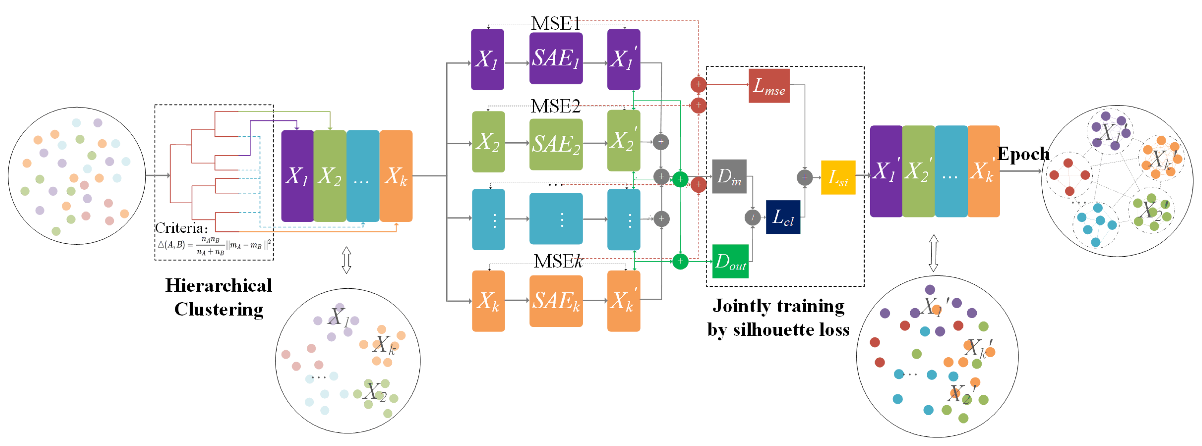
SiSAE, a novel detection model comprised of hierarchical clustering, silhouette loss, and joint SAE, is proposed in light of the existing technology and is depicted in Figure 3. Both are articulated in this section.

3.1. Hierarchical Clustering

This study employed the unsupervised hierarchical clustering algorithm to first treat each sample as a block and then use the similarities between blocks to merge them to achieve the set number of clusters. In this way, the raw data were divided into many blocks, with the size of each block being significantly related to the number of clusters and distance measures. In addition, the clustering method was used to maintain each cross-block of data as far as feasible from a particular perspective, giving each block a distinct characteristic and reducing the need to acquire redundant characteristics. In the meantime, this allowed each block to convey more information than would be achieved by utilizing the complete block of data directly. The cross-block information can be represented more effectively and transparently than the total. Within each data block, the clustering algorithm was used to keep data points as close as feasible, allowing the model to rapidly acquire the representation of inner-block.
Given a training data matrix X R n m , where n is the number of samples and m is the number of variables in a sample, the cluster can be expressed as
X 1 , X 2 , . . . , X k = f ( X )
where X 1 R n m 1 represents the first block of data, X 2 R n m 2 represents the second block of data, X k R n m k represents the l t h block of data, and the equation m 1 + m 2 + . . . + m k = m is always satisfied. f is an algorithm for clustering. After clustering the inputs, the distance between the data inner-block of the inputs is closer, and the gap between the center of each block of data is further away.

3.2. Silhouette Loss

Given a training data matrix X R n m , where n is the number of samples and m is the number of variables in a sample, the input X utilizes the SAE model to reconstruct the output X R n m by minimizing the MSE loss function. Figure 2 depicts the fine-tuning stage. However, explicitly rebuilding the input with all multivariate data is inaccurate due to the omission of local and cross-local information. This work introduces a novel loss function called silhouette loss in order to maximize the use of local and cross-local information in the data.
In this study, silhouette loss, which consists of the mean squared error and contrast error, was used as the loss function. MSE loss was employed to bring the output value as close as possible to that of the input. Each parallel SAE model contained an MSE loss, which enablds the correct reconstruction of each block of data. The total MSE was computed as follows:
L m s e = 1 2 n i = 1 k j = 1 n i ( x i , j x i , j ) T ( x i , j x i , j )
where k is the total number of blocks, n i is the amount of data in the i t h block, n = n 1 + n 2 + . . . + n k , x i , j is the j t h input data of the i t h block, x i , j is the j t h output data of the i t h block.
However, MSE loss does not take into consideration the relationship of distribution between the variables, making it harder for the model to understand the more hidden information. Therefore, contrast loss is intended to ensure that models fully account for local and cross-local information. Contrast loss consists of two components, which are D i n and D o u t , respectively. D i n represents the distance between data within the inner-block of the outputs, whereas D o u t represents the distance between the centre of each block of the outputs. D i n is determined as follows:
D i n = i = 1 k 1 n j n i ( x i , j x ¯ i ) T ( x i , j x ¯ i )
where x ¯ i is the output center of the i t h block. The other is described as
D o u t = i = 1 k j = 1 , j i k ( x ¯ i x ¯ j ) T ( x ¯ i x ¯ j )
where x ¯ i is the center of i t h block, and x ¯ j is the center of j t h block. Then, the contrast loss is expressed as
L c l = D i n D o u t
The function of D i n is to decrease the data distance in the inner-block of the output, while the function of D o u t is to increase the data distance in the cross-block of the output. The final calculation for the silhouette loss function is as follows:
L s i = L m s e + L c l
To ensure the same distribution of inputs and outputs during the minimization of the L s i loss function, the D i n of the outputs gradually decreases, while the D o u t increases. The L s i loss function is capable of learning the relationship between each block’s output and input. Meanwhile, L c l is utilized to efficiently learn cross-block information and further extract inner-block information.

3.3. Joint Stacked Autoencoder

The total k clustered data blocks are input into the respective SAE model in parallel and are jointly trained by the sihouette loss function. The size of the model is proportional to the various blocks of the inputs. The scale of the model is supposed to be greater for blocks with more variables and smaller for blocks with fewer variables. Given k blocks of input data, they are reconstructed as the output X 1 , X 2 , . . . , X k of the corresponding size. The l t h block input X l , l ( 1 , 2 , . . . k ) is numerically identical to the l t h output X l , l ( 1 , 2 , . . . k ) as much as possible by the MSE loss function. In addition, contrast loss is applied between output blocks to replicate the inputs’ data distribution.
Generally, a process error lies outside the acceptable range of variables or parameters. Monitoring a process can be accomplished by assessing the variables’ deviations from their usual states. The l t h SAE model was trained on the l t h block data to obtain the feature H l and residual X l X l The following statistic T 2 was constructed by utilizing a hidden representation of consisting of each block.
T 2 = H T 1 H
where H = [ H 1 , H 2 , . . . , H k ] , 1 is the variance matrix of H . The index describes the model variation over time. The other statistic S P E is the square reconstruction error of X and is described as follows:
S P E = ( X X ) T ( X X )
where X = [ X 1 , X 2 , . . . , X k ] , X = [ X 1 , X 2 , . . . , X k ] . The statistic reflects the differences between actual process data and SAE model-generated data. Equation (17) computes the contribution of the j t h variable in the i t h block, and variables with larger deviations contribute increasing amounts to the fault.
Δ i , j = | x i , j x i , j |
The thresholds for the statistics should be computed after the monitoring statistics have been established. Because no prior information on the data distribution was available, the KDE approach was utilized to establish the thresholds. In the meantime, the moving average filter was used to increase the final detection performance due to the effect of noise.
Remark 1.
Two of the most essential measures in process monitoring, the false detection rate (FDR) and the detection rate (DR), were used to evaluate the performance of the monitoring approach.
Definition 1.
Given n normal samples, the F D R may be demonstrated as
F D R = n a b n o r m a l | n o r m a l n n o r m a l × 100 %
which expresses that the percentage of normal samples that are incorrectly identified as fault samples, where n n o r m a l is the number of normal samples and n f a l s e | n o r m a l is the number of samples that are misdetected as fault samples.
Definition 2.
Given n abnormal samples, D R can be characterised as
D R = n a b n o r m a l | a b n o r m a l n a b n o r m a l × 100 %
which is the proportion of abnormal samples misdetected as normal samples, where n a b n o r m a l is the number of abnormal samples and n a b n o r m a l | a b n o r m a l is the number of undetected fault samples.

4. Experiment and Analysis

To demonstrate the superiority and efficacy of the proposed method, we employed the TE benchmark process and an industrial semiconductor process. In this section, we describe the use of the SiSAE model and a large number of additional sophisticated methods (MSPM methods, deep learning methods) to detect TE process problems. In addition, we detail ablation experiments that were performed to confirm the feasibility of the SiSAE model for enhancing the DR. Lastly, semiconductor industry data are used to demonstrate our methods further.

4.1. Case Study on Tennessee Eastman Process

In chemical engineering, the TE process is an extensively utilized benchmark platform for process monitoring. The detailed structure, process variables, and industrial processes of the TE process can be determined [27,28]. In this study, a total of 33 variables were used, including 22 continuous process measurement variables and 11 manipulated variables (except for agitation, which was not manipulated), and 21 different process faults were incorporated for process monitoring. The details of both are described in [29]. During the 48 h of operation, 33 variables were measured at 3-min intervals, and each fault was introduced after 8 h. Both the training and test data consisted of 960 samples, with the test data containing defect values from the 160th sample.
There were a total of 33 variables, which were separated into three blocks of 21, 5, and 7 variables, respectively. The first 80% of the samples were used for training, while the remaining 20% were utilized for validation. The activation function of all layers was “tanh”, and the gradient descent optimization algorithm was Adam with the learning rate ε set to 0.001. The batch size was set to 10, while the epoch was set to 2000. In addition, the early stopping strategy was implemented to effectively prevent overfitting, and adaptive adjustment of the learning rate approach was implemented to further enhance the network’s performance. The final mean squared error with contrast for the validation section was 0.07041. The monitoring specifics of two classical faults, faults 11 and 19, were elaborated to demonstrate the monitoring capability of our approaches.
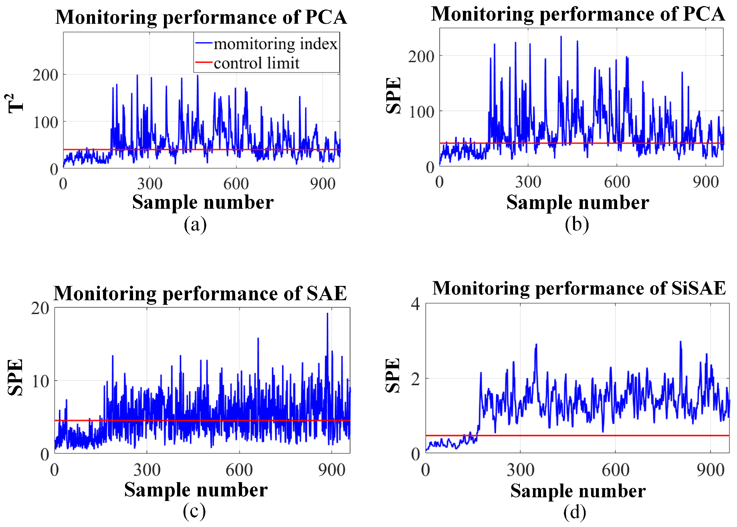
Fault 11 was a random variation in the inlet temperature of the reactor’s cooling water that was caused by the introduction of a random variable. Figure 4 depicts the monitoring performance based on the PCA, SAE, and SiSAE model. When the statistic reached the red control threshold, the sample was deemed to be abnormal. PCA’s T 2 and S P E statistics were able to detect 65.63% and 72.5% of faults for fault 11. The S P E statistic of a single SAE model with the same number of neurons as the combined SAE was able to detect 83.63% of faults, and our strategy enhanced the DR to 95.88%, which is the highest of several methods.
Fault 19 was an unknown fault in the TE process that was difficult for most monitoring approaches to detect due to its similarity to normal conditions. Figure 5 depicts the monitoring outcomes of PCA, SAE, and our approach for Fault 19. The detection performance indicates that it was difficult for the PCA, and SAE approaches to effectively detect the fault. However, our proposed method was able to detect nearly all fault samples of Fault 19.
In Table 1 and Table 2, the DR and FDR of our S P E statistic for the faults are compared with those of other approaches. The findings obtained by monitoring with multiple MSPM and deep network approaches, including PCA, KPCA [24], AE [30], M-DBN [24], LE-DBN [31], SAE, and SiSAE are presented.
The highest DR and lowest FDR are highlighted in bold. Due to the fluctuating nature of widely detectable faults, such as 1, 2, 6, 7, 8, 12, 13, 14, 17, and 18, virtually all approaches invariably produced DR values exceeding 90%. For small faults, such as 3 and 15, the DR achieved by most methods was considerably low. For faults 4, 5, 6, 7, 10, 11, 14, 16, 19, and 20, our technique produced the highest DR, and the detection performance was significantly enhanced, particularly for faults 11, 19, 20. In addition, the average DR was the highest, with our method demonstrating a low FAR, as shown in Table 2. The comparison with previous methods reveals that the proposed method offers a superior and practicable monitoring performance.
In addition, a series of ablation studies, depicted in Table 3, were used to validate the efficacy of the numerous proposed sections. To make the ablation experiment comparable, the SAE and SiSAE models employed the same number of neurons. The SAE’s encoder structure was 33-108-60-20, and the combined SAE comprised three SAE models with the following encoder structures: 21-50-33-17, 5-17-11-7, and 7-25-17-11. Compared with the basic SAE, the SiSAE mainly uses (1) the multiblock strategy of hierarchical clustering to extract local information, (2) the silhouette loss function to mine silhouette information, and (3) the moving average strategy to reduce the effects of noise. The main methods used in the ablation experiment were SAE, SAE+ (1), SAE+ (1)+ (2), and SAE+ (1)+ (2)+ (3), i.e., SiSAE. The results are listed in Table 3. The SiSAE model was found to be approximately 7 percentage points more accurate than the SAE. The combination of (1), (2) and (3) improved the results by around 3, 1, and 4 points, respectively.

4.2. Case Study of the Semiconductor Industrial Process

To further demonstrate the efficacy and viability of the proposed strategy, data from the semiconductor industry were used to validate the monitoring performance.
The data included four components or layers that were created by four different types of semiconductor machine parameter settings. Each layer was compoed of 16 spectra, with each spectrum containing 971 variables, giving a total of 15,536 variables. A correlation analysis method, called the maximal information coefficient (MIC), can extract linear and nonlinear features from data, and it was used to calculate the correlation between input and output variables. Each variable of the spectra required an MIC score, and a threshold was set to choose suitable variables. Finally, the 7 spectra with the most suitable variables were selected from all 16 spectra as the input. Seven of these spectra, which were more relevant to the output of the correlation analysis, were used for training and detection to minimize training requirements.
The first data layer was referred to as aluminum-90 (AL-90) and was considered typical data in this study. Other data layers were referred to as shallow trench isolation (STI), floating gate (FG), metal 1 tungsten (M1W), and metal 2 tungsten (M2W) and were considered abnormal data, i.e., faults 1–4. There were roughly 450 normal samples contained within the layer of AL-90’s five data slots (slot 1–5). The STI, FG, M1W, and M2W layers had around 300 samples.
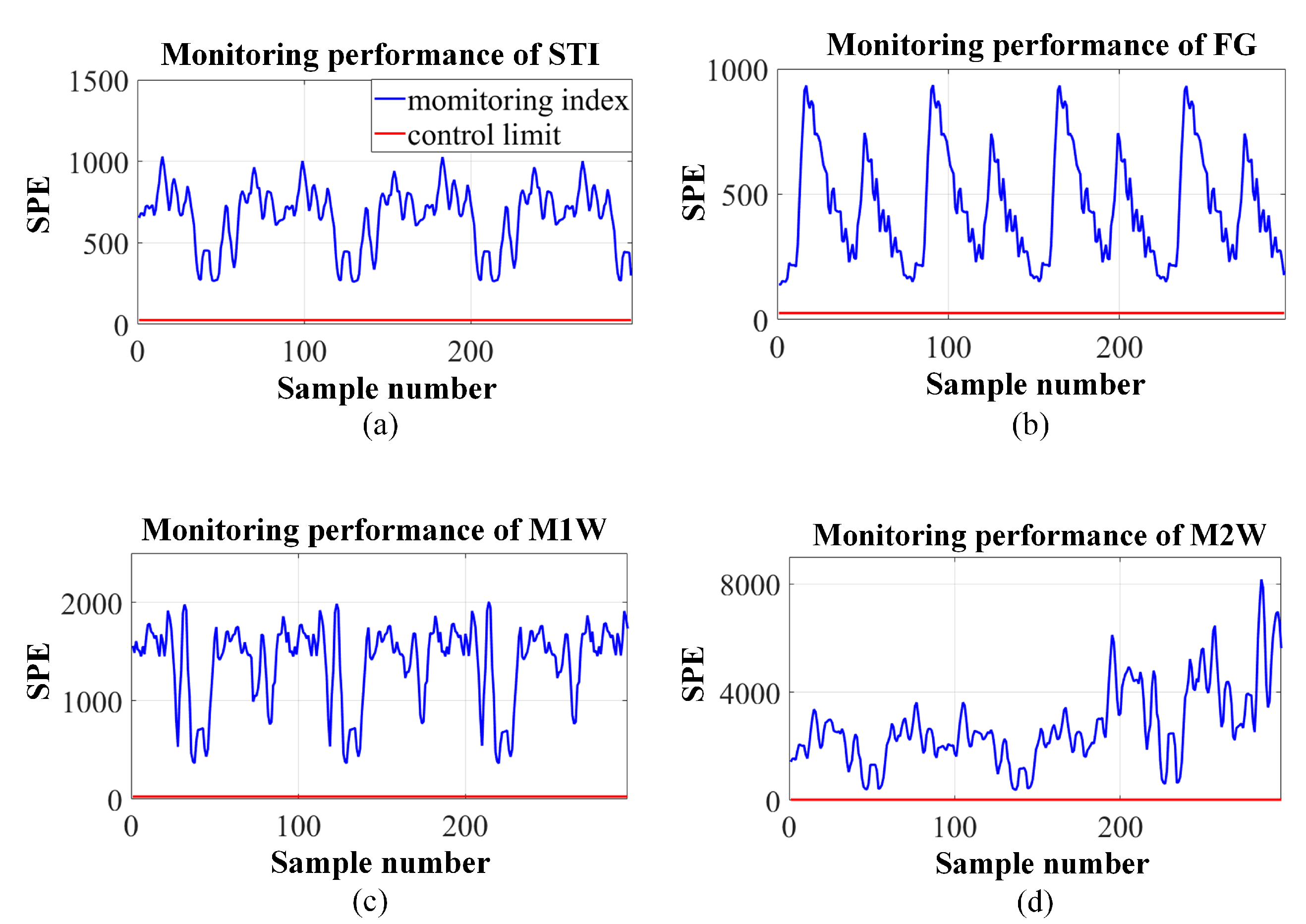
The AL-90 slot1 was trained to obtain the SPE statistic of control limits for monitoring the FDR of other AL-90 slots and the DR of the M1W, M2W, STI, and FG layers. The clustering technique was used to divide a total of 6797 variables into three blocks. The parallel three SAE models used the same input-1500-750-350 structure. In addition, the optimization algorithm, training strategy, etc. were identical to the TE process. The monitoring results are illustrated in Figure 6 and Figure 7. The outcome demonstrates that the FDR was zero in AL-90 and that all anomalous samples were detectable in M2W, M1W, STI, and FG. In summary, semiconductor industrial data were used to demonstrate the practicability and effectiveness of the proposed method.

5. Conclusions

In this research, a novel model called the silhouette stacked autoencoder that takes the local and cross-local information of the data into consideration was proposed for fault detection. In this model, the hierarchical clustering algorithm was first used to partition the raw data into several blocks, creating similar information inside each block and dissimilar information between blocks. Then, the silhouette loss function was designed to fully extract additional local and cross-local information. Finally, several blocks of data were fed in parallel to the corresponding appropriately sized SAE models, which were then trained to represent the information between data blocks. Twenty-one types of faults and ablation studies in the TE process were used to prove the efficacy and superiority of our proposed method. In addition, the FDR of other slots in AL-90 was zero, and all anomalous samples were detected in the M2W, M1W, STI and FG layers using semiconductor industrial data, demonstrating the effectiveness of the proposed approach. An improvement in performance was demonstrated from the perspective of the loss function and joint training. We will further analyze the effect of interactive information between data blocks by the attention mechanism from the perspective of the model. In addition, we will further analyze the impact of noise in the data on blocking results and the detection performance.

Author Contributions

Conceptualization, J.Y.; Methodology, H.R. and J.Y.; Software, H.R. and J.Y.; Validation, H.R.; Formal Analysis, H.R. and J.Y.; Resources, F.S., Z.L. and X.Y.; Data Curation, H.R. and J.Y.; Writing—Original Draft Preparation, H.R.; Writing-Review and Editing, J.Y., Z.L. and F.S.; Visualization, H.R.; Supervision, J.Y. and Z.L.; Project Administration, F.S., X.Y.; Funding Acquisition, Z.L. and J.Y. All authors have read and agreed to the published version of the manuscript.

Funding

National Natural Science Foundation of China under Grant 62173077, Grant 62203118, “Xing Liao Ying Cai” Program under Grant XLYC1907073, and National Key Research and Development Program of China under Grant 2020YFB1713700.

Institutional Review Board Statement

Not applicable.

Informed Consent Statement

Not applicable.

Data Availability Statement

Not applicable.

Conflicts of Interest

The authors declare no conflict of interest. The funders had no role in the design of the study, in the collection, analyses, or interpretation of data, in the writing of the manuscript, or in the decision to publish the results.

References

  1. You-Jin, P.; Fan, S.K.S.; Chia-Yu, H. A Review on Fault Detection and Process Diagnostics in Industrial Processes. Processes 2020, 8, 1123. [Google Scholar]
  2. Qin, S.J. Survey on data-driven industrial process monitoring and diagnosis. Annu. Rev. Control 2012, 36, 220–234. [Google Scholar] [CrossRef]
  3. Yin, S.; Xiao, B.; Ding, S.X.; Zhou, D. A review on recent development of spacecraft attitude fault tolerant control system. IEEE Trans. Ind. Electron. 2016, 63, 3311–3320. [Google Scholar] [CrossRef]
  4. Ge, Z.; Song, Z.; Gao, F. Review of recent research on data-based process monitoring. Ind. Eng. Chem. Res. 2013, 52, 3543–3562. [Google Scholar] [CrossRef]
  5. Tatara, E.; Çinar, A. An intelligent system for multivariate statistical process monitoring and diagnosis. ISA Trans. 2002, 41, 255–270. [Google Scholar] [CrossRef]
  6. Zhang, K.; Shardt, Y.A.; Chen, Z.; Peng, K. Using the expected detection delay to assess the performance of different multivariate statistical process monitoring methods for multiplicative and drift faults. ISA Trans. 2017, 67, 56–66. [Google Scholar] [CrossRef]
  7. Ge, Z.; Song, Z.; Ding, S.X.; Huang, B. Data mining and analytics in the process industry: The role of machine learning. IEEE Access 2017, 5, 20590–20616. [Google Scholar] [CrossRef]
  8. Yin, S.; Ding, S.X.; Haghani, A.; Hao, H.; Zhang, P. A comparison study of basic data-driven fault diagnosis and process monitoring methods on the benchmark Tennessee Eastman process. J. Process Control 2012, 22, 1567–1581. [Google Scholar] [CrossRef]
  9. Jaffel, I.; Taouali, O.; Harkat, M.F.; Messaoud, H. Moving window KPCA with reduced complexity for nonlinear dynamic process monitoring. ISA Trans. 2016, 64, 184–192. [Google Scholar] [CrossRef]
  10. Pilario, K.E.; Shafiee, M.; Cao, Y.; Lao, L.; Yang, S.H. A review of kernel methods for feature extraction in nonlinear process monitoring. Processes 2019, 8, 24. [Google Scholar] [CrossRef] [Green Version]
  11. Heo, S.; Lee, J.H. Statistical process monitoring of the Tennessee Eastman process using parallel autoassociative neural networks and a large dataset. Processes 2019, 7, 411. [Google Scholar] [CrossRef]
  12. Hinton, G.E.; Salakhutdinov, R.R. Reducing the dimensionality of data with neural networks. Science 2006, 313, 504–507. [Google Scholar] [CrossRef] [Green Version]
  13. Han, B.; Ji, S.; Wang, J.; Bao, H.; Jiang, X. An intelligent diagnosis framework for roller bearing fault under speed fluctuation condition. Neurocomputing 2021, 420, 171–180. [Google Scholar] [CrossRef]
  14. Han, B.; Zhang, X.; Wang, J.; An, Z.; Jia, S.; Zhang, G. Hybrid distance-guided adversarial network for intelligent fault diagnosis under different working conditions. Measurement 2021, 176, 109197. [Google Scholar] [CrossRef]
  15. Sakurada, M.; Yairi, T. Anomaly detection using autoencoders with nonlinear dimensionality reduction. In Proceedings of the MLSDA 2014 2nd Workshop on Machine Learning for Sensory Data Analysis, Gold Coast, QLD, Australia, 2 December 2014; pp. 4–11. [Google Scholar]
  16. Jiang, G.; Xie, P.; He, H.; Yan, J. Wind turbine fault detection using a denoising autoencoder with temporal information. IEEE/Asme Trans. Mechatron. 2017, 23, 89–100. [Google Scholar] [CrossRef]
  17. Yuan, X.; Huang, B.; Wang, Y.; Yang, C.; Gui, W. Deep learning-based feature representation and its application for soft sensor modeling with variable-wise weighted SAE. IEEE Trans. Ind. Informatics 2018, 14, 3235–3243. [Google Scholar] [CrossRef]
  18. Cheng, F.; He, Q.P.; Zhao, J. A novel process monitoring approach based on variational recurrent autoencoder. Comput. Chem. Eng. 2019, 129, 106515. [Google Scholar] [CrossRef]
  19. Kohonen, J.; Reinikainen, S.P.; Aaljoki, K.; Perkiö, A.; Väänänen, T.; Höskuldsson, A. Multi-block methods in multivariate process control. J. Chemom. A J. Chemom. Soc. 2008, 22, 281–287. [Google Scholar]
  20. Cherry, G.A.; Qin, S.J. Multiblock principal component analysis based on a combined index for semiconductor fault detection and diagnosis. IEEE Trans. Semicond. Manuf. 2006, 19, 159–172. [Google Scholar] [CrossRef]
  21. Li, W.; Zhao, C.; Gao, F. Linearity evaluation and variable subset partition based hierarchical process modeling and monitoring. IEEE Trans. Ind. Electron. 2017, 65, 2683–2692. [Google Scholar] [CrossRef]
  22. Yu, J.; Yan, X. Data-feature-driven nonlinear process monitoring based on joint deep learning models with dual-scale. Inf. Sci. 2022, 591, 381–399. [Google Scholar] [CrossRef]
  23. Jiang, Q.; Yan, S.; Cheng, H.; Yan, X. Local–global modeling and distributed computing framework for nonlinear plant-wide process monitoring with industrial big data. IEEE Trans. Neural Netw. Learn. Syst. 2020, 32, 3355–3365. [Google Scholar] [CrossRef] [PubMed]
  24. Yu, J.; Yan, X. Modeling large-scale industrial processes by multiple deep belief networks with lower-pressure and higher-precision for status monitoring. IEEE Access 2020, 8, 20439–20448. [Google Scholar] [CrossRef]
  25. Li, Z.; Tian, L.; Jiang, Q.; Yan, X. Distributed-ensemble stacked autoencoder model for non-linear process monitoring. Inf. Sci. 2021, 542, 302–316. [Google Scholar] [CrossRef]
  26. Sun, J.; Shi, H.; Zhu, J.; Song, B.; Tao, Y.; Tan, S. Self-attention-based Multi-block regression fusion Neural Network for quality-related process monitoring. J. Taiwan Inst. Chem. Eng. 2022, 133, 104140. [Google Scholar] [CrossRef]
  27. McAvoy, T.; Ye, N. Base control for the Tennessee Eastman problem. Comput. Chem. Eng. 1994, 18, 383–413. [Google Scholar] [CrossRef]
  28. Downs, J.J.; Vogel, E.F. A plant-wide industrial process control problem. Comput. Chem. Eng. 1993, 17, 245–255. [Google Scholar] [CrossRef]
  29. Li, Y.; Ma, F.; Ji, C.; Wang, J.; Sun, W. Fault Detection Method Based on Global-Local Marginal Discriminant Preserving Projection for Chemical Process. Processes 2022, 10, 122. [Google Scholar] [CrossRef]
  30. Jang, K.; Hong, S.; Kim, M.; Na, J.; Moon, I. Adversarial autoencoder based feature learning for fault detection in industrial processes. IEEE Trans. Ind. Informatics 2021, 18, 827–834. [Google Scholar] [CrossRef]
  31. Yu, J.; Yan, X. Layer-by-layer enhancement strategy of favorable features of the deep belief network for industrial process monitoring. Ind. Eng. Chem. Res. 2018, 57, 15479–15490. [Google Scholar] [CrossRef]
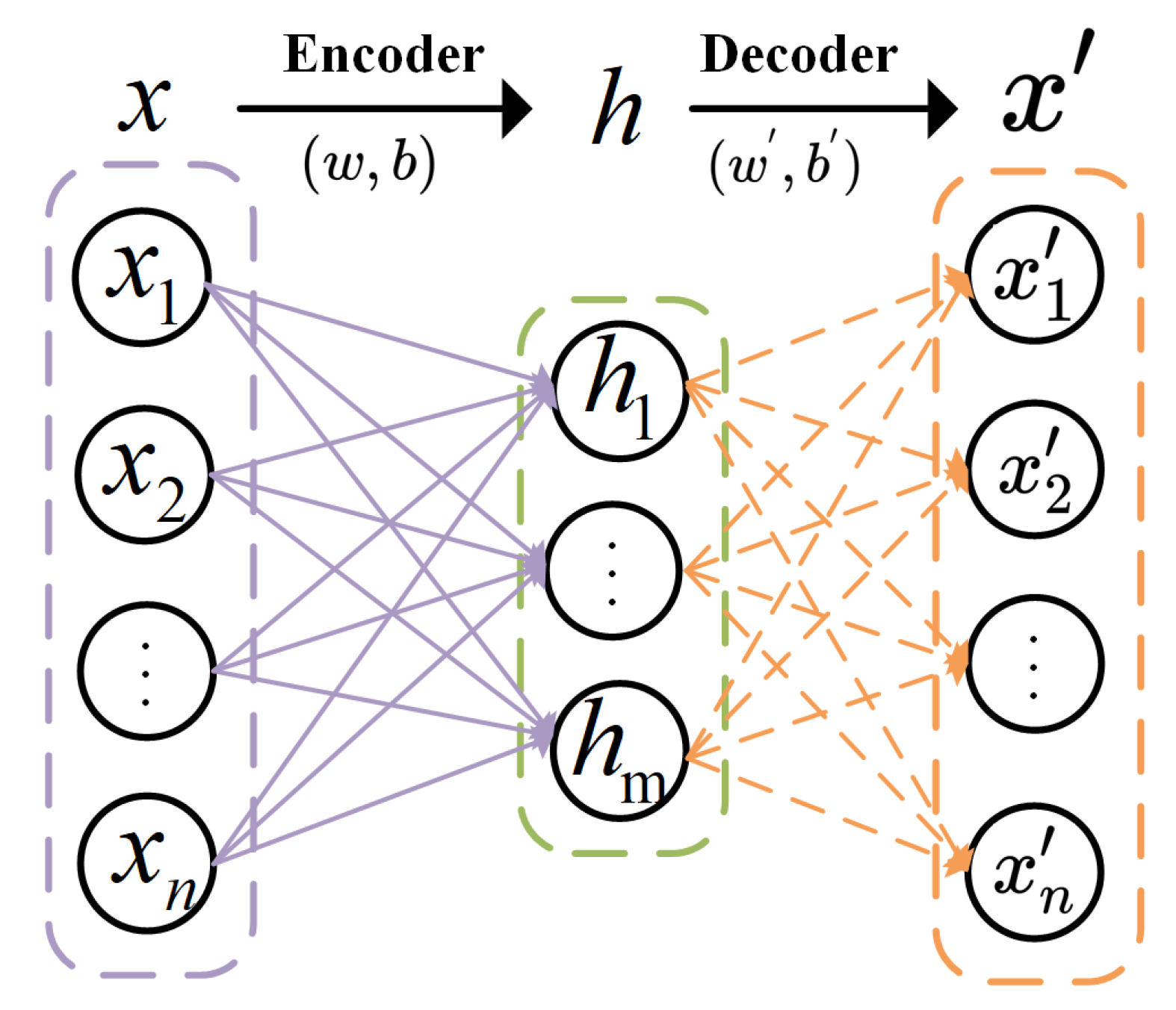
Figure 1. The structure of AE.
Processes 10 02408 g001
Figure 2. The training process of SAE.
Processes 10 02408 g002
Figure 3. The detection model of SiSAE.
Processes 10 02408 g003
Figure 4. Monitoring results obtained with PCA, KPCA, SAE, and SiSAE for fault 11. (a) is the performance of T 2 of PCA, (bd) is the performance of S P E of PCA, SAE, and SiSAE, respectively.
Processes 10 02408 g004
Figure 5. Monitoring results obtained with PCA, KPCA, SAE, and SiSAE for fault 19. (a) is the performance of T 2 of PCA, (bd) is the performance of S P E of PCA, SAE, and SiSAE, respectively.
Processes 10 02408 g005
Figure 6. Monitoring results of AL-90. (ad) is the performance of S P E of SiSAE on slot 2,3,4, and 5, respectively.
Processes 10 02408 g006
Figure 7. Monitoring results of other layers. (ad) is the performance of S P E of SiSAE on STI, FG, M1W, and M2W, respectively.
Processes 10 02408 g007
Table 1. Detection Rate for All Faults in the TE Process.
Fault No.PCAKPCAAELE-DBNM-DBNSAESiSAE
10.9950.010.9981.001.001.0000.999
20.9860.030.9900.980.990.9860.985
30.2190.090.2590.020.170.0590.176
40.8130.840.9941.001.001.0001.000
50.4080.170.4981.001.001.0001.000
61.0000.011.0001.001.001.0001.000
71.0000.781.0001.001.001.0001.000
80.9900.310.9900.970.990.9810.986
90.1790.070.2550.010.020.0440.011
100.5740.610.6790.760.780.6850.909
110.7250.660.8440.890.860.8360.959
120.9980.350.9940.991.000.9910.998
130.9510.130.9640.960.970.9610.968
141.0000.371.0001.001.001.0001.000
150.2140.140.3150.170.230.1000.271
160.5010.540.6360.690.590.5560.886
170.9200.330.9550.980.960.9790.976
180.9150.020.9230.910.920.9100.910
190.1940.130.4780.910.950.6430.999
200.5850.480.6930.740.800.6920.870
210.4510.440.6090.340.520.4930.525
Average0.6960.310.7660.7770.7980.7580.830
Table 2. Average False Detection Rate for All Faults in the TE Process.
Fault No.PCAKPCAAELE-DBNM-DBNSAESiSAE
Average0.0850.0270.08130.0160.0330.0460.039
Table 3. Ablation Experiments with the SiSAE Model.
MethodSAESAE+(1)SAE+(1)+(2)SiSAE
Average0.7580.7840.7920.83
Publisher’s Note: MDPI stays neutral with regard to jurisdictional claims in published maps and institutional affiliations.