A Dynamic Principal Component Analysis and Fréchet-Distance-Based Algorithm for Fault Detection and Isolation in Industrial Processes

Abstract

Fault Detection and Isolation (FDI) methodology focuses on maintaining safe and reliable operating conditions within industrial practices which is of crucial importance for the profitability of technologies. In this work, the development of an FDI algorithm based on the use of dynamic principal component analysis (DPCA) and the Fréchet distance $\left({\delta }_{dF}\right)$ metric is explored. The three-tank benchmark problem is studied and utilized to demonstrate the performance of the FDI method for six fault types. A DPCA transformation for the system was established, and fault detection was conducted based on the Q statistic. Fault isolation is also of critical importance for proper intervention to mitigate fault effects. To identify the type of detected faults, the fault responses within the PC subspace were analyzed using the ${\delta }_{dF}$ metric. The use of the Fréchet distance metric for the isolation of faults combined with DPCA for feature extraction is a novel technique to the best of the authors’ knowledge that provides a robust computational tool with low computational cost for FDI purposes that fits well into the Industry 4.0 framework.The robustness and sensitivity of the method was validated for a wide variety of signal-to-noise ratio (SNR) conditions, with findings indicating a possible average false and missed alarm rate of 0.1 and a macro-averaged F-score above 0.8 in all cases.

1. Introduction

Fault detection and isolation (FDI) has become a key issue in industrial process management to ensure safety, profitability and sustainable operation of industrial plants. Faults as mentioned by Venkatasubramanian et al. are departures from an acceptable range of a specific variable associated with a process [1]. Thus, faults are symptomatic changes within a process, and they are the results of underlying events called root causes. In this work, the goal was to develop a data-based method for timely fault detection and isolation in industrial systems to enhance the framework of FDI.

Many industrial accidents, such as the Bhopal disaster or the Texas oil refinery fire, already accentuate the importance of the FDI methodology [2,3]. Still the importance of developing robust and sensitive FDI methods to prevent large scale catastrophes is a key challenge in the chemical industry. A good example of this is the case of the explosion at the West Fertilizer facility. In this incident, an ammonium nitrate storage of a fertilizer production plant exploded in West Texas in April of 2013 leading to fifteen fatalities, numerous fires within the facility and considerable damage to residential areas [4]. Another recent incident is the Kaohsiung explosion. In August of 2014 a 4 km long section of subterranean gas pipelines exploded near Kaohsiung, Taiwan, devastating residential areas built above them [5]. Finally, one of the most recent events was the accidental release of styrene from a polymer production facility, also known as the Vizag gas leak. The event which led to the accidental release in August of 2020 was a self-polymerization runaway reaction in a styrene storage tank in a facility of LG polymers located near Vizag, India. The release of gas resulted in severe health damage to the population of the surrounding area and significant environmental damage [6].

In response to these accidents, model and data-based FDI methods have been developed over the last decades. The classification of methods in this way, based on the type of process knowledge used to isolate faults, is arbitary and unique to the FDI literature [1].

Model-based techniques utilize quantitative or qualitative descriptions of the system to distinguish between faulty and normal operating conditions. FDI with these methods is generally achieved by means of residual generation techniques. Residuals are signals which indicate discrepancies between expected system behaviour derived from the process model and the behaviour of the actual system. Provided that the system model is accurate, these differences are due to the presence of noise, disturbances or process faults. With mathematical models being popularly used for FDI, the observed system is generally described using state–space or input–output representation [7]. The most common methods of residual generation based on state–space and input–output models include observer-based, filter-based and parity equation-based approaches, with the first two usually using state–space representations of the investigated system and the latter using either.

Since both utilized model types are most often linear in nature, recent studies have mainly focused on extending them to linear discrete time-varying (LDTV) systems as a way to approximate the behaviour of nonlinear systems [8]. Li et al. utilized a generalized fault detection filter to tackle the problem of optimal residual generation in LDTV systems with uncertain observations [9]. Nemati et al. developed a nonlinear observer for the supervision of a satellite’s flight. During the procedure of FDI development, they considered the presence of model uncertainty, input and environmental disturbances [10]. Wang et al. employed a finite-horizon robust filtering method designed using $H_{\infty }$ optimization. They applied their method to the problem of distributed FDI in LDTV multi-agent systems with varying dynamics and bounded model uncertainties [11]. Wu et al. utilized the parity space method through a recursive algorithm to supervise LDTV systems subject to multiplicative noise. They employed a novel FDI performance metric to design the residual generator and gave limits for the uncertainty of residual values in the framework of stochastic analysis [12]. Despite their robustness and the significant focus of academic research on them, model-based FDI methods are seldom implemented in practice due to the high level of mathematical knowledge necessary to formulate them. Additionally, even though many developments have been made to extend the framework of model-based FDI to nonlinear systems, issues such as the handling of multiplicative faults and noise are still of critical importance and a serious hurdle [7].

Data-based methods which utilize large amounts of operation data to extract features of various faults from observable data have garnered significant interest over the years. These approaches include statistic methods, artificial intelligence, neural network structures, etc., which are used for feature extraction from operation data and acquisition of knowledge used to characterize and classify different types of system behaviour [7]. Data-based methods have become attractive due to a multitude of causes. These include their generally easy implementation, their good compatibility with the Industry 4.0 framework which provides easy access to an abundant amount of process data and the lack of need for an explicit process model for FDI [7].

Zhang et al. utilized convolutional neural networks with wide first-layer kernels for the FDI of raw vibration signals. Their method achieved good isolation performance (100% in the observed cases) and showed strong resistance to the presence of measurement noise [13]. Toma et al. developed a motor current signal-based FDI method for electrical and mechanical systems. They employed statistical feature extraction combined with a genetic algorithm on observed data to achieve the extraction of features and the reduction of feature dimensionality. Subsequently, they pinpointed and isolated faults using a neural network, decision tree and random forest and evaluated the performance of each classifier [14]. Lee et al. used wavelet transform combined with a neural network trained using the particle swarm optimization algorithm. They showed the performance of the algorithm during the FDI of motors [15]. While a promising direction of research, neural networks suffer from several shortcomings which include the need for reliable and abundant process data for their training, their often complex structure and, depending on the determined structure, the computational cost of training the networks [7].

Among the statistic methods for FDI, principal component analysis (PCA) and its derived methods have garnered great popularity. PCA is a method which is convenient for statistical process monitoring (SPM). It aims to reduce the complexity of multivariate data through a projection onto a subspace (referred to as the principal component (PC) subspace) in which the maximum variance of the original variable space is retained with minimal dimensionality [16,17]. The original PCA method achieved this reduction in dimensionality through a linear transformation [18]. Over time, many alternatives for PCA have been developed, most focusing on adapting the method to data sets obtained from nonlinear processes or introducing approaches for adaptive thresholding. A few notable of these approaches are the techniques of kernel PCA, nonlinear PCA, recursive PCA, moving window PCA and dynamic PCA (DPCA) [19].

An example of nonlinear PCA can be found in the work of Kramer where an autoassociative neural network with a bottleneck layer was trained and its capabilities for data dimensionality reduction displayed [20]. Mansouri et al. developed a kernel principal-component-analysis-based algorithm that utilized the generalized likelihood ratio test for FDI in a continuous stirred unit [21]. Li et al. proposed the use of recursive PCA for monitoring processes with changing behaviour through efficient updating of the process variable matrix and adaptive adjustments of principal component number and confidence limits for statistical testing [22]. Ammiche et al. utilized moving window PCA to update control limit thresholds for dynamic processes and reduce the false alarm rate [23].

DPCA originates from the works of Ku et al. who proposed an extension of the traditional PCA method for dynamic systems monitored within industrial processes. Since PCA is mainly applicable for cross-correlated data sets, its use for supervision of dynamic processes can result in inaccurate statistic process monitoring. The short sampling times for variable data acquisition within process industries result in the presence of significant auto-correlation within the data that the traditional static PCA method is unfit to handle. The method proposed by Ku et al. solved this problem by introducing the DPCA method in which the data set is enhanced with time-lag-shifted versions of the original variables. The resulting Hankel matrix which contains the lag-shifted data can be subject to the same steps used for traditional PCA. By appropriately choosing the number of lags, dynamic as well as static relationships between the data can be captured [24].

The use of DPCA for FDI purposes has a well-established background in the literature and is a contemporary and relevant direction of research. The main focus nowadays lies in optimizing the fault detection capabilities of DPCA and enhancing it to minimize false alarm rate (FAR) and missed alarm rate (MAR). Another relevant direction lies in the combination of PCA with various classifiers to pinpoint the root causes of faults in addition to detecting the presence of anomalies. Rato and Seis, for example, developed an FDI method based on DPCA using decorrelated residuals and displayed the usefulness of their method on the Tennessee Eastman benchmark problem [25]. Huang and Yan developed a new process-monitoring algorithm using DPCA and dynamic independent component analysis combined with Bayesian inference [26]. Vanhatalo et al. proposed novel ways to determine the optimal lag number of DPCA. Their method observes the behaviour of the eigenvalues of the lagged autocorrelation and partial autocorrelation matrices [17]. Buonoua and Bakdi proposed the use of a dynamic kernel PCA (DKPCA) method for monitoring nonlinear dynamical systems. They utilized the theory of nonlinear fractal dimensions to optimize the DPCA structure [27]. The reason for the extensive focus on PCA and DPCA in the field of academic research is due to a multitude of causes. As the previous examples have shown, nonlinear systems, due to the data-based nature of the algorithms, fit well into the Industry 4.0 framework, and the absence of an explicit process model makes their mathematical description simple. In this context, it is also important to note that due to its popularity, many methods have been developed to make PCA more applicable even under unfavourable conditions, such as the characterization of systems from a data set with scarce or missing data. Missing data, for example, is an issue for many data-based techniques. Brute force solutions, such as deleting samples with missing values or substituting a mean estimate value for the variable, will, however, either result in loss of information or the deterioration of the covariance structure within the data. For PCA and the DPCA, many techniques have been developed to resolve such issues. Such methods can be found, for example, in the work of Stanimirova et al. who proposed an expectation maximization SPCA for the handling of missing data and outliers within PCA [28]. Dray and Josse in their review article compiled the possible solutions for dealing with missing data in PCA. Among the strategies, they observed methods for imputation of missing values prior to standard PCA, PCA algorithms that skip missing values and algorithms which consider these missing values during iterative procedures [29]. In their work, Kwon et al. proposed an algorithm which combines traditional DPCA with a self-consistency observation concept for developing a DPCA transformation for time-series data with missing values. In their work, they compared the approach with previously existing methods such as imputation techniques during Monte Carlo simulations [30]. Another important aspect which showcases the versatility of PCA is the multitude of methods which allow the extension of PCA for different scales denoted as multi-scale PCA (MSPCA). This is necessary since in most dynamic processes the system behaviour is strongly influenced by events which occur at different locations and localizations in both frequency and time or are stochastic in nature meaning that their power spectrum changes with both time and/or frequency [31]. Misra et al. proposed an MSPCA method for the extraction of event contributions to process data on corresponding scales based on the wavelet transformation [32] and enhanced it with a multi-scale fault identification scheme. Sophian et al. applied PCA on different scales for the observation of sub-surface defects through results obtained from testing through pulsed Eddy currents. They utilized their method to differentiate between samples that suffered from surface cracks, sub-surface cracks and sub-surface metal loss [33]. Lau et al. developed a method which combined MSPCA with a neuro-fuzzy inference system for feature extraction of a dynamic process and learning fault-symptom correlations from the derived features. They validated their method by showcasing it for the supervision of the Tennessee Eastman benchmark problem [34].

In recent years, there has been a rise in the use of trajectory similarity metrics as tools of fault isolation in the framework of FDI. Among them, the discrete Fréchet distance as a similarity metric has garnered special research interest. The discrete Fréchet distance describes the distance between two polygonal curves which takes ordering of points along the curve into account. Its use in isolation lies in analyzing time series of system variables and pointing out similarities between real-time data and various known fault signal responses. As an example of its use, Weng et al. proposed a method based on the discrete Fréchet distance to analyze current transformers and differentiate between internal and external fault currents [35]. Huang et al. used a two-stage turnout fault diagnosis method for railways based on the Fréchet distance [26].

Conversely, the application of trajectory similarity methods for fault classification in FDI is a promising direction due to the simplicity of said methods compared to other classifiers, such as neural networks, support vector machines, etc. One of the factors which could be limiting for its application though is the large amount of observed variables within a technological system. Selecting the optimal variables for observation is highly dependent on the fault types which are taken into consideration since observation of changes within all variables is computationally inefficient and hinders online diagnosis.

Our key idea in this work is the use of DPCA for detecting the presence of abnormalities within a dynamic system while simultaneously pinpointing the root causes of the anomalies through a data classification technique based on the discrete Fréchet distance metric. The application of DPCA provides dimensionality reduction for the data set which makes both multivariate statistical tests for fault detection and trajectory similarity calculations for fault isolation computationally less expensive and suitable for online fault diagnosis.

The algorithm uses input–output data of a process to establish a DPCA model with optimized lag number to reduce dimensionality within the data set and pinpoint outliers. The Q statistic is then employed to identify irregular data points belonging to faults. Within the PC subspace, the Fréchet distance metric is used to characterize similarity of registered abnormalities to a predetermined fault library and select the best possible match for each fault instance. The efficiency of the method has been validated using simulated data gathered from a three-tank benchmark problem. FDI capabilities have been characterized using False Alarm Rate (FAR) and Missed Alarm Rate (MAR) metrics, while classification accuracy for fault isolation has been evaluated based on the F score. The results show that the method exhibits good FDI capabilities with low computational cost, easy implementation and proper robustness.

The contribution of our work to the FDI methodology includes:

• A novel application of the Fréchet distance metric combined with DPCA to isolate process abnormalities and identify their root causes.
• Reduction of computational cost for the Fréchet distance calculations between reference and measured fault trajectories.
• A sensitive and robust FDI method with simple implementation and high accuracy that greatly fits into the Industry 4.0 framework.

2. Methods

In this section, we wish to give an overview of the PCA and DPCA methods as well as the Fréchet distance metric. After establishing the mathematical background of the methods, the proposed FDI algorithm will be discussed in detail.

2.1. Theory of PCA and DPCA

PCA proposes a method for the dimensionality reduction of a data set while maintaining maximum of the variance contained in the original variables. Consider a data set denoted by $\mathbf{X}\in {\mathbb{R}}^{n\times p}$ with n observations and p variables. For PCA, the columns of $\mathbf{X}$ are centered and scaled to have a mean of zero and unit variance. The centered and scaled $\mathbf{X}$ matrix shall be denoted as $\tilde{\mathbf{X}}$. The linear transformation to obtain the PCs from the centered data set can be obtained in various ways. Possible methods are through the eigenvalue decomposition (EVD) or the singular value decomposition (SVD) of the covariance matrix of $\tilde{\mathbf{X}}$. Alternatively, iterative methods such as the Nonlinear Iterative Partial Least Squares (NIPALS) algorithm may also be utilized. In the following, we will discuss the EVD-based algorithm for obtaining the PCs. For the transformation, the sample covariance matrix $\mathbf{V}\in {\mathbb{R}}^{p\times p}$ of $\tilde{\mathbf{X}}$ must be obtained. Due to the centering procedure, $\mathbf{V}$ may be calculated according to Equation (1).

$$\mathbf{V}=\frac{1}{n-1}{\tilde{\mathbf{X}}}^T\tilde{\mathbf{X}}$$

(1)

Following this, we obtain the EVD of the covariance matrix $\mathbf{V}$ according to Equation (2), where $\mathbf{P}\in {\mathbb{R}}^{\mathbf{p}\times \mathbf{p}}$ is a matrix containing the eigenvectors of $\mathbf{V}$, while $\mathsf{\Lambda }\in {\mathbb{R}}^{\mathbf{p}\times \mathbf{p}}$ is a diagonal matrix containing the eigenvalues of $\mathbf{V}$.

$$\mathbf{V}=\mathbf{P}\mathsf{\Lambda }{\mathbf{P}}^T$$

(2)

It can be shown that the eigenvectors of $\mathbf{V}$ point to the directions of maximum variance within the space of the original data set. The degree of variation explained in the direction of each eigenvector is proportional to the absolute value of its corresponding eigenvalue. By ordering the eigenvectors based on the absolute value of their corresponding eigenvalues in descending order, we obtain the matrix $\tilde{\mathbf{P}}$. The percentage of retained variance within each eigenvector $\left({\tilde{v}}_i,i=1,\dots ,p\right)$ compared to the original data set may be calculated. After this, the amount of cumulative variance to be retained $\left(\theta \right)$ may be chosen based on the scree plot of the calculated eigenvalues. The optimal number of PCs to be retained $\left(a\right)$ can be calculated according to Equation (3) provided that ${\sum }_{i=1}^p{\tilde{v}}_i\ge \theta$ holds true.

$$a=arg\underset{i}{min}{\left(\sum _{i=1}^p{\tilde{v}}_i-\theta \right)}^2$$

(3)

After calculating the number of PCs to be retained, the matrix $\tilde{\mathbf{P}}$ can be adjusted to contain only the necessary eigenvectors. This new matrix will be referred to as ${\tilde{\mathbf{P}}}_{\mathbf{a}}\in {\mathbb{R}}^{\mathbf{p}\times \mathbf{a}}$. The PCA transformation is then realized in the form of Equation (4) with $\mathbf{PC}\in {\mathbb{R}}^{n\times a}$, where optimally, $a\ll p$ holds true.

$$\mathbf{PC}=\tilde{\mathbf{X}}{\tilde{\mathbf{P}}}_{\mathbf{a}}$$

(4)

The reduced data set can retain most of the original variance coded within the data by choosing a high value of $\theta$. If chosen properly, the remaining $p-a$ eigenvectors account for the variation due to noise within the original data set. The PCA data decomposition model thus takes the form shown in Equation (5), where matrix $\mathbf{E}\in {\mathbb{R}}^{n\times p}$ is the prediction error.

$$\tilde{\mathbf{X}}=\mathbf{PC}{\tilde{\mathbf{P}}}_{\mathbf{a}}^T+\mathbf{E}$$

(5)

After dimensionality reduction, control statistics such as Hotelling’s $T^2$ statistic or the Q-statistic can be used for system supervision [24].

The Q-statistic, also known as Squared Prediction Error (SPE), provides a measure for the prediction error of the PCA model for a given data point. The Q-statistic can be calculated according to Equation (6), where $\mathbf{I}\in {\mathbb{R}}^{p\times p}$ is a unit matrix with appropriate dimensions [36].

$$Q=\left(\tilde{\mathbf{X}}-\mathbf{PC}{\tilde{\mathbf{P}}}_{\mathbf{a}}^T\right){\left(\tilde{\mathbf{X}}-\mathbf{PC}{\tilde{\mathbf{P}}}_{\mathbf{a}}^T\right)}^T={\tilde{\mathbf{X}}}^T\left(\mathbf{I}-{\tilde{\mathbf{P}}}_{\mathbf{a}}{\tilde{\mathbf{P}}}_{\mathbf{a}}^T\right)\tilde{\mathbf{X}}$$

(6)

A control metric for the Q-statistic has been proposed by Jackson and Mudholkar [36]. For a given confidence level, $\alpha$ control limits for Q values are calculated according to Equation (7).

$$Q_{\alpha }={\theta }_1{\left[1+\frac{c_{\alpha }\sqrt{2{\theta }_2{h}_0^2}}{{\theta }_1}+\frac{{\theta }_2{h}_0\left(h_0-1\right)}{{\theta }_1^2}\right]}^{\frac{1}{h_0}}$$

(7)

In Equation (7), $c_{\alpha }$ is the deviate belonging to the upper $1-\alpha$ percentile of the standard normal distribution, while ${\theta }_i$ and $h_0$ are metrics derived from polynomial sums of the $p-a$ eigenvalues of the covariance matrix of the data. If the value of Q exceeds the defined control limit, the associated data point can be regarded as an outlier of the statistic.

As was stated previously, PCA is useful for reducing the dimensionality of cross-correlated variables and creating a set of new orthogonal observation variables. However, the traditional form of PCA, also known as static PCA, has issues when observing the behaviour of dynamic systems. Process data is usually taken with small sampling time, resulting in major auto-correlation within the variables. To alleviate this problem, Ku et al. proposed the use of DPCA. In DPCA, the data matrix $\mathbf{X}$ is enhanced by adding in the time-lag-shifted variants of the observed variables, resulting in a Hankel-matrix structure as shown in Equation (8) [24].

$$\mathbf{X}=\left[\begin{array}{cccccccc}{x}_1\left(1\right)& x_1\left(2\right)& \dots & x_1(l+1)& \dots & x_p\left(1\right)& \dots & x_p(l+1)\\ x_1\left(2\right)& x_1\left(3\right)& \dots & x_1(l+2)& \dots & x_p\left(2\right)& \dots & x_p(l+2)\\ ⋮& ⋮& \ddots & ⋮& \dots & ⋮& \ddots & ⋮& \\ x_1(n-l)& x_1(n-l+1)& \dots & x_1\left(n\right)& \dots & x_p(n-l)& \dots & x_p\left(n\right)\end{array}\right]$$

(8)

After altering the data matrix in this way, auto-correlation between variables can be transformed into cross-correlation. After employing the same steps as with traditional PCA on the enhanced data set, a more accurate set of PCs can be calculated [24]. In the proposed algorithm, DPCA is utilized to recognize the presence of abnormalities based on statistical measures. In the isolation step, a classification algorithm employing the discrete Fréchet distance metric is utilized to categorize and isolate recognized fault signals and identify their root causes. The isolation step adheres to the following logic:

• Unknown fault inputs within a system result in specific system responses.
• The dynamics and gain of specific fault responses are dependent on the type and magnitude of the fault signal.
• The characteristic response to a system fault within the PC subspace will be unique if faults are observable and independent on the fault input magnitude.

2.2. The Fréchet Distance Metric

The Fréchet distance $\left({\delta }_{dF}\right)$ is a measure of similarity between two polygonal curves that takes into account the location and ordering of points along the curves. Eiter and Mannila provided a way of computation for the discrete Fréchet distance between two curves, also known as the coupling distance [37]. For measuring the similarity between two arbitrary curves, they are approximated as polygonal curves. Let the two curves to be compared be defined as sets of point $N:\left[0,n\right]\to T_f$ and $M:\left[0,m\right]\to T_l$. The sequence of end points for each line segment is denoted by $\sigma \left(N\right)=\left(u_1,u_2,\dots ,u_{n-1}\right)$ and $\sigma \left(M\right)=\left(v_1,v_2,\dots ,v_{m-1}\right)$ respectively. The set of all possible combinations between the end points of the polygonal curves $\left(H\right)$ is defined in Equation (9).

$$\mathbf{H}=\sigma \left(N\right)\times \sigma \left(M\right)$$

(9)

Couplings between the two curves are sequences of distinct pairs from H which respect the ordering of points in both curves. The length of a possible coupling between the two curves is denoted by $\parallel L\parallel$ which corresponds to the length of the longest link within the defined coupling. $\parallel L\parallel$ is calculated according to Equation (10). In the equation, the metric d stands for a chosen distance metric of the two sequences, which is most often the Euclidean distance.

$$\begin{array}{ccc}\hfill \parallel L\parallel =maxd\left(u_{a,i},v_{b,i}\right),& & \mathrm{where}i=1,\dots ,m-1\hfill \end{array}$$

(10)

The discrete Fréchet distance is defined as the minimum length of all possible couplings between the two polygonal curves as seen in Equation (11) [37].

$$\begin{array}{ccc}\hfill {\delta }_{dF}\left(N,M\right)=\min (\max d\left(u_{a,i},v_{b,i}\right)),& & \mathrm{where}i=1,\dots ,m-1\hfill \end{array}$$

(11)

2.3. The Proposed Algorithm

The proposed algorithm for FDI consists of two phases. These phases mostly match the general phases of PCA when utilized within the SPM procedure as noted by Vanhatalo et al. [17]. Phase I consists of acquiring a subset of process data about the system to be supervised under normal operating conditions. Using this data, the in-control DPCA model is established, and control limits for statistical measures are determined. In our case, this phase also includes the generation of a fault library for later isolation purposes. Phase II consists of real-time monitoring of the system which includes the detection and isolation of process abnormalities. The general steps of the FDI algorithm for both phases are shown in Algorithm 1 below.

Algorithm 1 Steps of the proposed FDI algorithm.

Phase 1—Establishing the DPCA model and fault library 1: procedureEstablishing the DPCA model 2:     Calculate l based on the algorithm proposed by Ku et al. [24] 3:     Compute the enhanced data matrix $\mathbf{X}\in {\mathbb{R}}^{\left(n-l\right)\times p\left(l+1\right)}$ 4:     Center and standardize the enhanced data matrix $($ 5:     Calculate $\mathbf{V}=\frac{1}{n-l-1}{\tilde{\mathbf{X}}}^T\tilde{\mathbf{X}}$ 6:     Calculate matrix $\tilde{\mathbf{P}}$ using EVD 7:     Determine a using the scree plot according to [24] 8:     Calculate ${\tilde{\mathbf{P}}}_{\mathbf{a}}$ 9: end procedure 10: procedureEstablishing the fault library 11:     Obtain data set ${\mathbf{X}}_f\in {\mathbb{R}}^{n\times p}$ containing system abnormalities F 12:     Compute $\mathbf{PC}$ values for the data $\mathbf{PC}={\tilde{\mathbf{X}}}_{\mathbf{f}}{\tilde{\mathbf{P}}}_{\mathbf{a}}$ 13:     Compute Q-statistic for the data set and isolate out of control points ${\mathbf{PC}}_f$ 14:     for each fault f do 15:         Calculate ${\mathbf{PC}}_n\left(f\right)=\frac{{\mathbf{PC}}_f}{max\parallel {\mathbf{PC}}_f\parallel }$ 16:     end for 17: end procedure     Phase 2—Online supervision of the process 18: procedureFault detection 19:     Obtain data set ${\mathbf{X}}_o\in {\mathbb{R}}^{n\times p}$ to be analyzed 20:     Compute $\mathbf{PC}$ values for the data $\mathbf{PC}={\tilde{\mathbf{X}}}_{\mathbf{o}}{\tilde{\mathbf{P}}}_{\mathbf{a}}$ 21:     Pinpoint outliers for a given confidence level using the Q-statistic 22:     Store data of outlier points within the PC subspace ${\mathbf{PC}}_o$ 23: end procedure  24: procedureFault isolation 25:     for each recognized individual fault signal $\left(F_o\right)$ within data set ${\mathbf{PC}}_o$ do 26:         for each reference fault stored within the fault library $P{C}_n\left(f\right)$ do 27:            Calculate ${\delta }_{dF}\left(P{C}_n\left(f\right),F_o\right)$ 28:            Define the unknown fault $F_o$ as $arg{min}_f\left({\delta }_{dF}\left(P{C}_n\left(f\right),F_o\right))\right)$ 29:         end for 30:     end for 31: end procedure

3. Case Study

The FDI capabilites of the proposed method have been tested using data gathered from the a priori model of the three-tank benchmark system displayed in Figure 1 [38]. This benchmark problem is well-known in the FDI framework. For this work, it was utilized due to the nonlinear nature of the system as well as the highly correlated process variables.

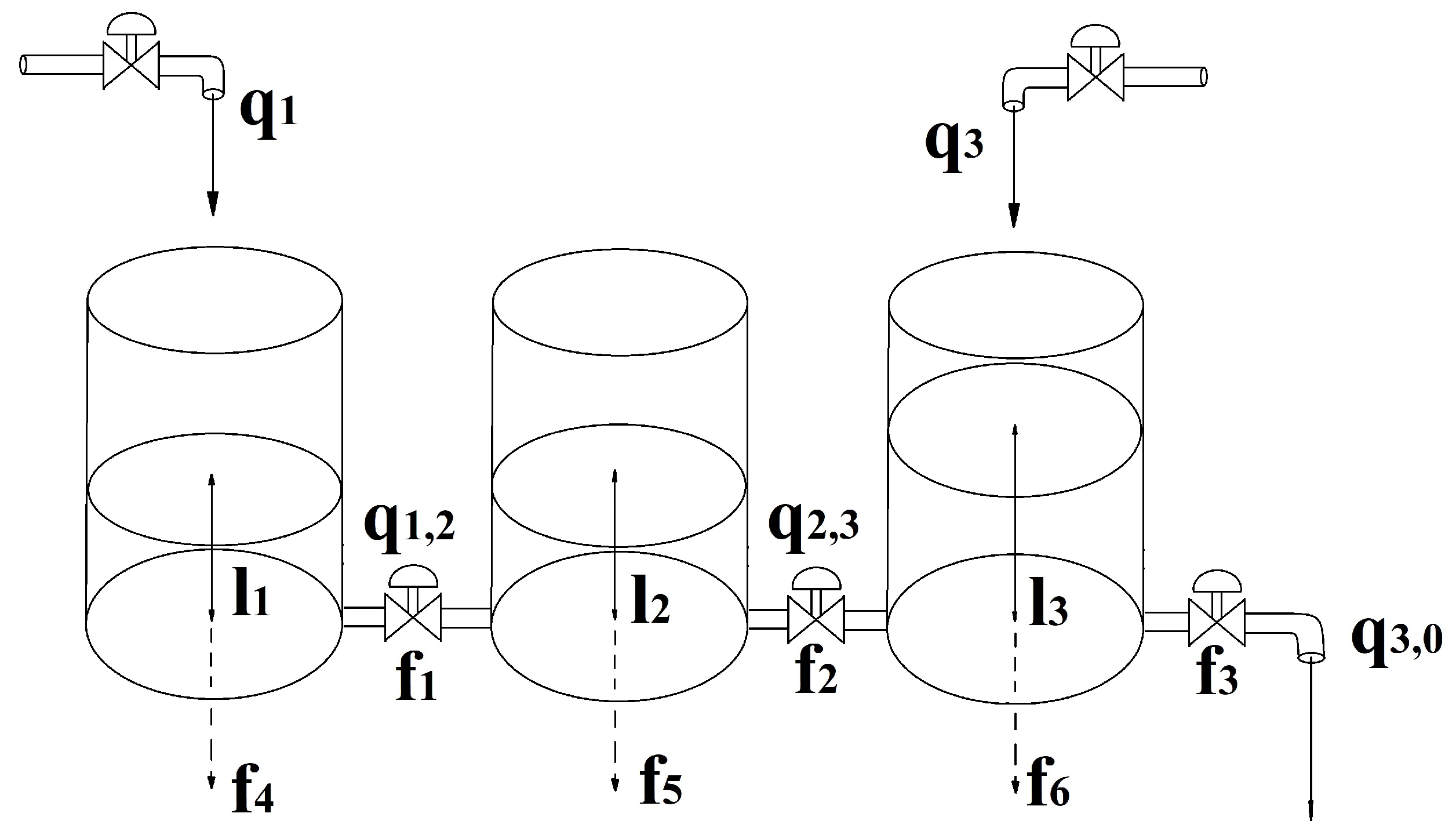
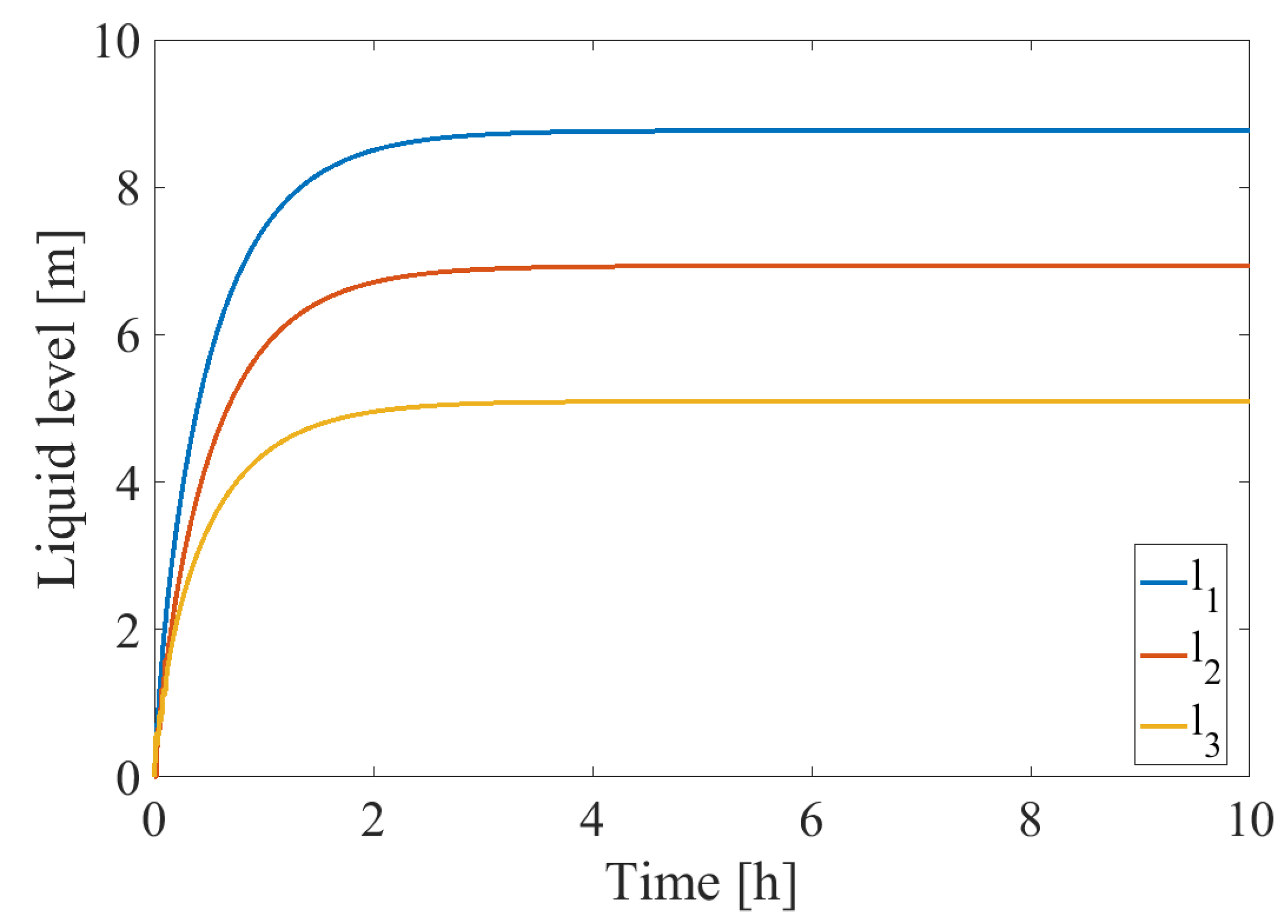
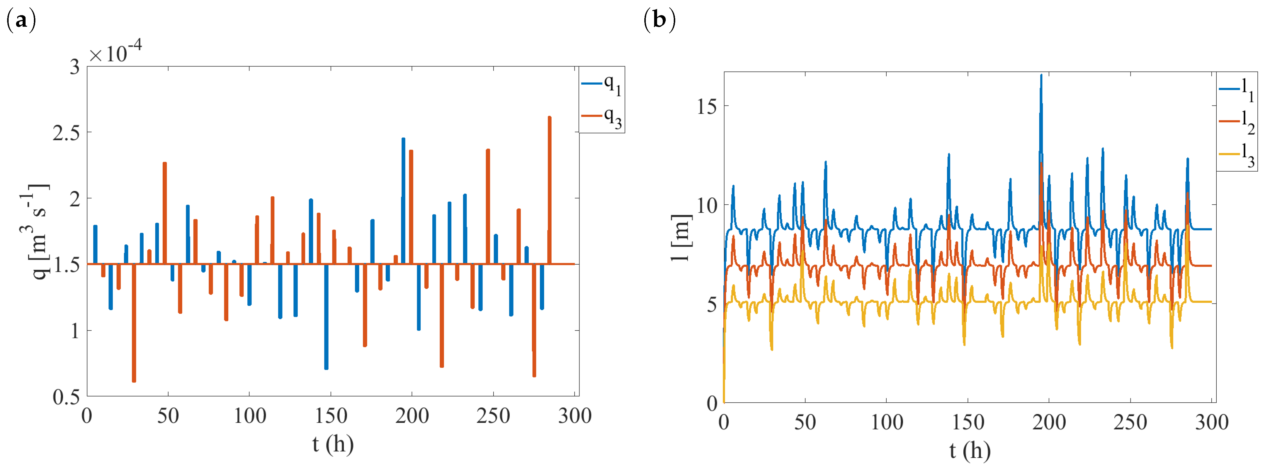
3.1. The Investigated System

The investigated system contains three interconnected cylindrical tanks in series with uniform cross section S. The outlet position of each tank is located at the bottom of the respective tank. Connections between the tanks are possible though flow within the cylindrical pipes connecting them all have cross section $S_n$. Inlet flow rates $q_1$ and $q_3$ are controlled through externally operated inlet valves.

The three measurable outputs of the system are the liquid levels in each tank $\left(l_1,l_2,l_3\right)$, while the measurable inputs that influence the levels are the inlet flow rates in the first and last tank $\left(q_1,q_3\right)$. Flow rates between the tanks are denoted by $q_{i,j}$, where i and j are indices of the connected tanks or the outside, respectively. The flow rates between tanks are dependent on the liquid level within each tank as well as the outflow coefficient ${\mu }_{i,j}$ which is a function of the valve position of the pipe segment.

Six possible faults within the system have been taken into account to validate the method. The first three involve the decrement of the outflow coefficients in each pipe segment $\left(f_1,f_2,f_3\right)$ that can be caused by build-up of sediment within the pipe segment or malfunction of the control valve. The latter three are the presence of leakages within each tank $\left(f_4,f_5,f_6\right)$.

To gather data about the system behaviour under various normal and irregular operating conditions, the first principle model of the system was established. The system of differential equations governing the liquid level within each tank is shown in Equation (12), provided that the cross sections of each tank are unchanged during the observation.

$$\begin{array}{cc}\hfill \frac{d{l}_1}{dt}& =\frac{1}{S}\left(q_1-q_{1,2}-q_{1,f}\right)\hfill \\ \hfill \frac{d{l}_2}{dt}& =\frac{1}{S}\left(q_{1,2}-q_{2,3}-q_{2,f}\right)\hfill \\ \hfill \frac{d{l}_3}{dt}& =\frac{1}{S}\left(q_3+q_{2,3}-q_{3,0}-q_{3,f}\right)\hfill \end{array}$$

(12)

Flow rates between tanks were calculated according to the set of equations described in Equation (13) based on Torriceli’s law.

$$\begin{array}{cccc}\hfill q_{i,j}& ={\mu }_{i,j}{S}_{n}sgn\left(l_i-l_j\right)\sqrt{2g\mid l_i-l_j\mid },\hfill & \hfill & i\ne 3\hfill \\ \hfill q_{3,0}& ={\mu }_{3,0}Sn\sqrt{2g{l}_3}\hfill \\ \hfill q_{i,f}& =f_{i+3}{\mu }_f{S}_f\sqrt{2g{l}_i}\hfill \end{array}$$

(13)

For the calculation of volumetric flow exiting the tank due to leakages $\left(q_{i,f}\right)$, the fault signals $f_{i+3}$ are assumed to be binary signals with value one if leakage is present within the tank and value of zero otherwise.

To obtain data about the system under normal operating conditions, simulations have been conducted with the model. A steady-state for the system has been chosen, and changes have been made to the input variables (the inlet flow rates) to assess the changes within water level in the tank. The acquired data were utilized thereafter to establish the DPCA transformation.

The operational parameters of the observed steady-state as well as the constructional parameters of the tank and parameters of possible faults are displayed in

Table 1. Operational and constructional parameters of the investigated system.

${\mathit{q}}_1\left[{\mathbf{m}}^3{\mathbf{s}}^{-1}\right]$	${\mathit{q}}_2\left[{\mathbf{m}}^3{\mathbf{s}}^{-1}\right]$	${\mathsf{\mu }}_{1,2}\left[-\right]$	${\mathsf{\mu }}_{2,3}\left[-\right]$	${\mathsf{\mu }}_{3,0}\left[-\right]$
$1.5\times {10}^{-4}$	$1.5\times {10}^{-4}$	0.5	0.5	0.6
${\mathbf{\mu }}_{\mathit{f}}\left[-\right]$	$\mathit{S}\left[{\mathbf{m}}^{\mathbf{2}}\right]$	${\mathit{S}}_{\mathit{p}}\left[{\mathbf{m}}^{\mathbf{2}}\right]$	${\mathit{S}}_{\mathit{f}}\left[{\mathbf{m}}^{\mathbf{2}}\right]$	${\mathit{l}}_{\mathit{i},\mathbf{0}}\left[\mathbf{m}\right]$
0.6	$1.5\times {10}^{-2}$	$5\times {10}^{-5}$	$5\times {10}^{-5}$	0

.

The dynamic change of the tank level within the system in the investigated steady-state and fault free circumstances is shown in Figure 2.

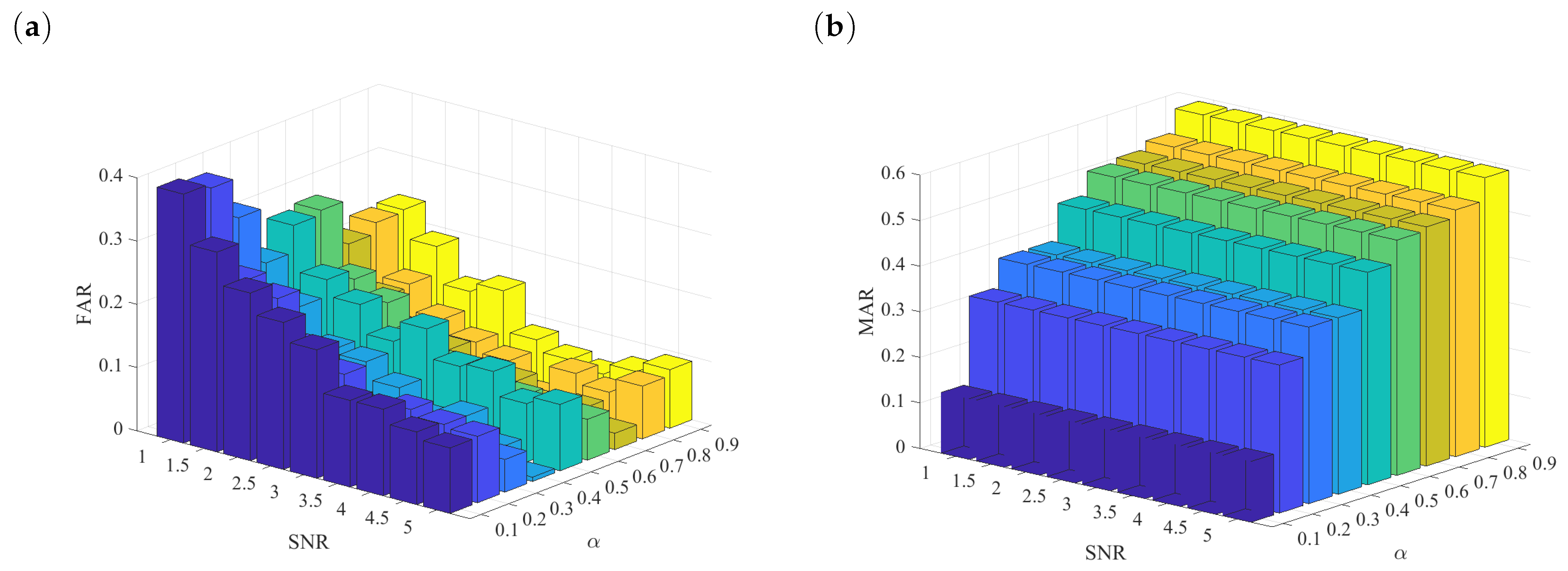
3.2. Performance Metrics

In our study, the false alarm rate (FAR) and missed alarm rate (MAR) metrics were used for evaluating the detection prowess of the method. To quantify the performance of the isolation algorithm based on the Fréchet distance metric, the macro-averaged F score was utilized. The equations to calculate the FAR and MAR metrics are shown in Equations (14) and Equation (15) [39]. The variables $FN,TP,FP$ and $TN$, respectively, refer to:

• Samples incorrectly classified as faults under normal operating conditions (FN-False Negative).
• Samples correctly classified under normal operating conditions (TP-True Positive).
• Samples incorrectly classified as normal under abnormal operating conditions (FP-False Positive).
• Samples correctly classified under abnormal operating conditions (TN-True Negative).

$$FAR=\frac{FN}{TP+FN}$$

(14)

$$MAR=\frac{FP}{TN+FP}$$

(15)

The F metric shows the harmonic mean of a classifier’s recall $\left(R\right)$ and precision $\left(P\right)$ ability. Equations (16)–(18) show the method for calculating $P,R$ and F for a multi-class problem [40].

$$P_c=\frac{{\sum }_{c=1}^{C}T{P}_c}{{\sum }_{c=1}^{C}T{P}_c+F{P}_c}$$

(16)

$$R_c=\frac{{\sum }_{c=1}^{C}T{P}_c}{{\sum }_{c=1}^{C}T{P}_c+F{N}_c}$$

(17)

$$F_c=\frac{2P_c{R}_c}{P_c+R_c}$$

(18)

4. Results

The results are presented sequentially based on the steps of the algorithm. First, to obtain the DPCA transformation, the system was observed near its steady-state operation point.

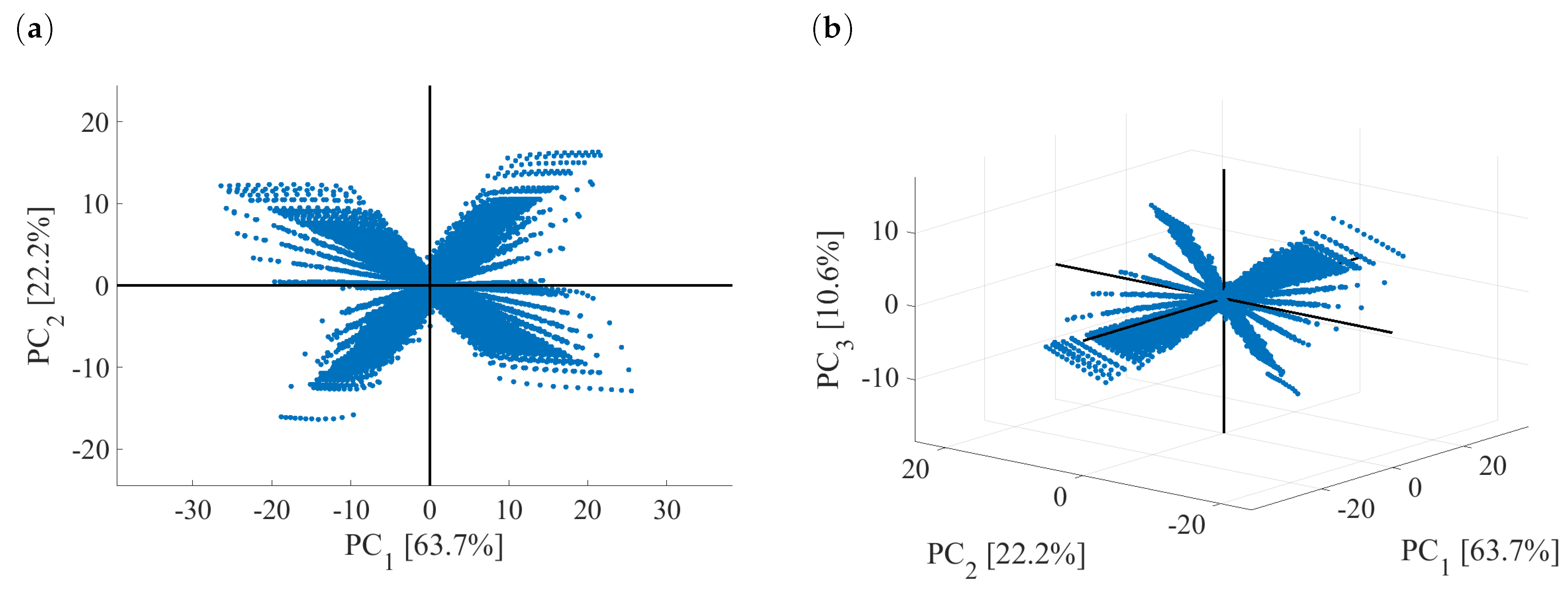
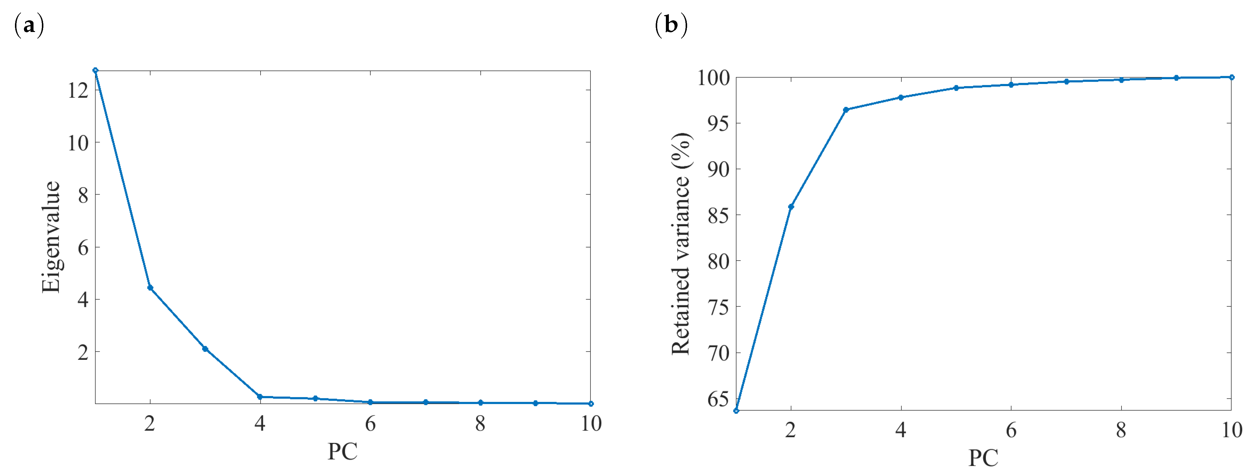
4.1. Development of DPCA Model

The system was observed in a time window of 300 h, with a sampling time of 120 s. During this time, 60 changes were made in the value of the input volumetric flow. The percentage deviation of the inputs from their steady-state values were calculated as random variables with a normal distribution of mean 0 and a variance of 0.25. The results of the data acquisition can be seen in Figure 3

Based on the observations, the DPCA model of the system was established. To do this, the lag number for the transformation had to be calculated. The optimal lag number was defined as three based on the algorithm proposed by Ku et al. [24]. For the estimation, the data matrix $\tilde{X}$ contained all the observable input and output variables $\left(q_1,q_3,l_1,l_2,l_3\right)$ and their time-shifted versions centered around the steady-state value of each observed variable. After calculating the DPCA transformation, the number of PCs was chosen. For this, the scree plot displaying the eigenvalues associated with each principal component of the transformation was investigated. The scree plot of the DPCA transformation as well as the cumulative variance retained for each PC can be seen in Figure 4.

By observing Figure 4a, it can be seen that the first three eigenvalues of the covariance matrix have significant magnitudes when compared to the remaining eigenvalues. Due to this, the PC number was chosen to be three, and the use of the remaining PCs was omitted. The cumulative retained variance within the PCs is shown in Figure 4b. It can be observed that the first three PCs encapsulate more than 95 % of the variance contained within the original data set.

After the transformation, the original data set was evaluated within the PC subspace. This is shown in Figure 5, where the axes show the percentage of the original data set’s variance contained within individual PC’s.

Figure 5a,b display the trajectories of changes within the PC subspace in 2D and 3D, respectively. The four observable trajectories within the data set correspond to positive and negative changes within the two input variables and the subsequent changes within the liquid levels in the three tanks observed in Figure 3. Points located at the origin in each representation correspond to values where the observed inputs and outputs are identical to their steady-state values. The dynamic changes appear as deviations from the origin that follow characteristic trajectories and return to the origin once the input variables return to their steady-state values, prompting the levels within the tanks to also return.

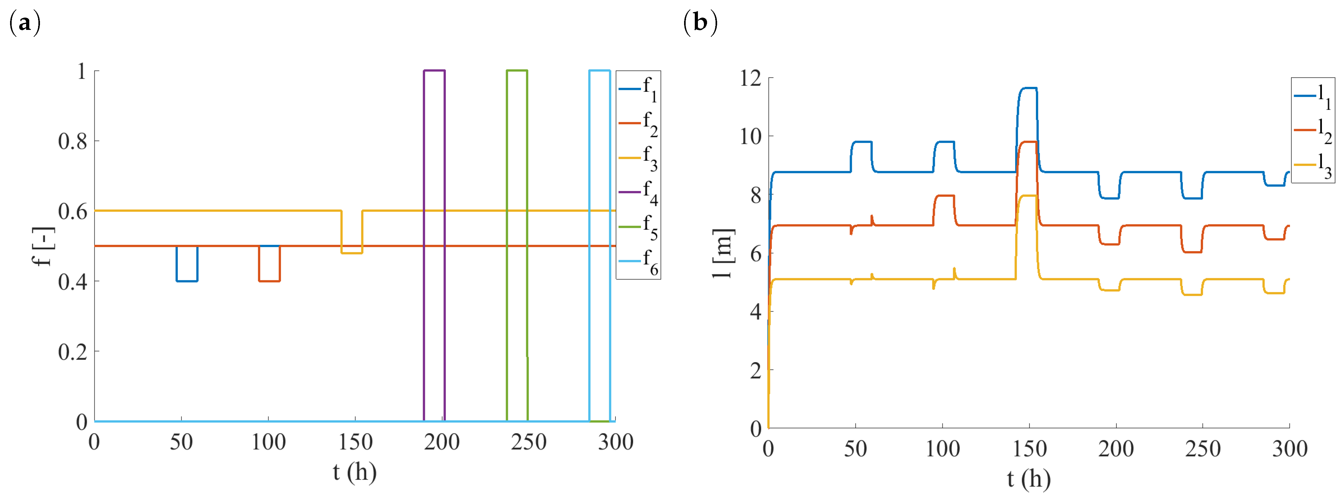
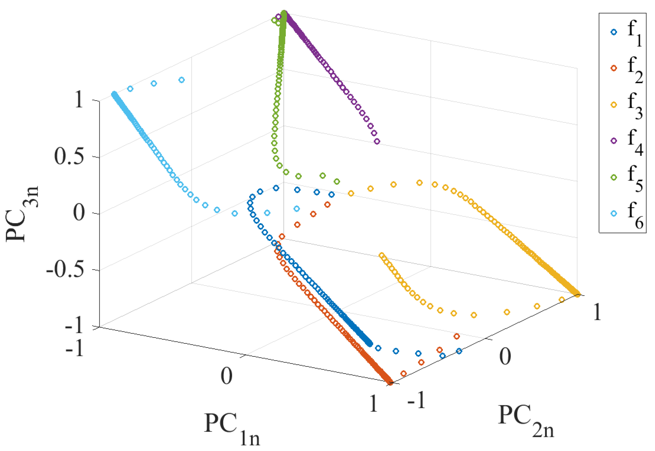
4.2. Fault Library Generation

After the DPCA transformation has been obtained, the behaviour of the system under the presence of the six possible faults is observed. The observed fault signals and the responses of the liquid levels within the three tanks can be seen in Figure 6.

The first three fault instances that can be seen in Figure 6a show the deviation of the flow coefficient from its steady-state value. The three latter fault instances show the presence of leakages in tanks one, two and three, respectively. The decrement of the flow coefficients shows similar tendencies. When the flow coefficient of a pipe segment decreases, the level within the tanks before the afflicted pipeline rises, while the levels of the tanks after it remain mostly unaffected. Leakage,s however, affect the level in each of the three tanks regardless of where they occurred. The DPCA transformation that was obtained from observing the in-control system was applied to the data set containing the faults. After that, the Q-statistic with confidence level $\alpha =0.1$ was employed to extract data points that belonged to faulty system behaviour. Trajectories of the isolated faults are displayed in Figure 7.

The trajectories shown in Figure 7 have been normalized within the PC subspace normalized to the interval $[-1,1]$.

Since the magnitude of fault trajectories within the PC subspace depends on the magnitude of the fault input, it was necessary to decouple the obtained trajectories from the magnitude of the fault signal for the isolation steps. After obtaining the trajectories of the observed faults, Phase I of the algorithm is concluded.

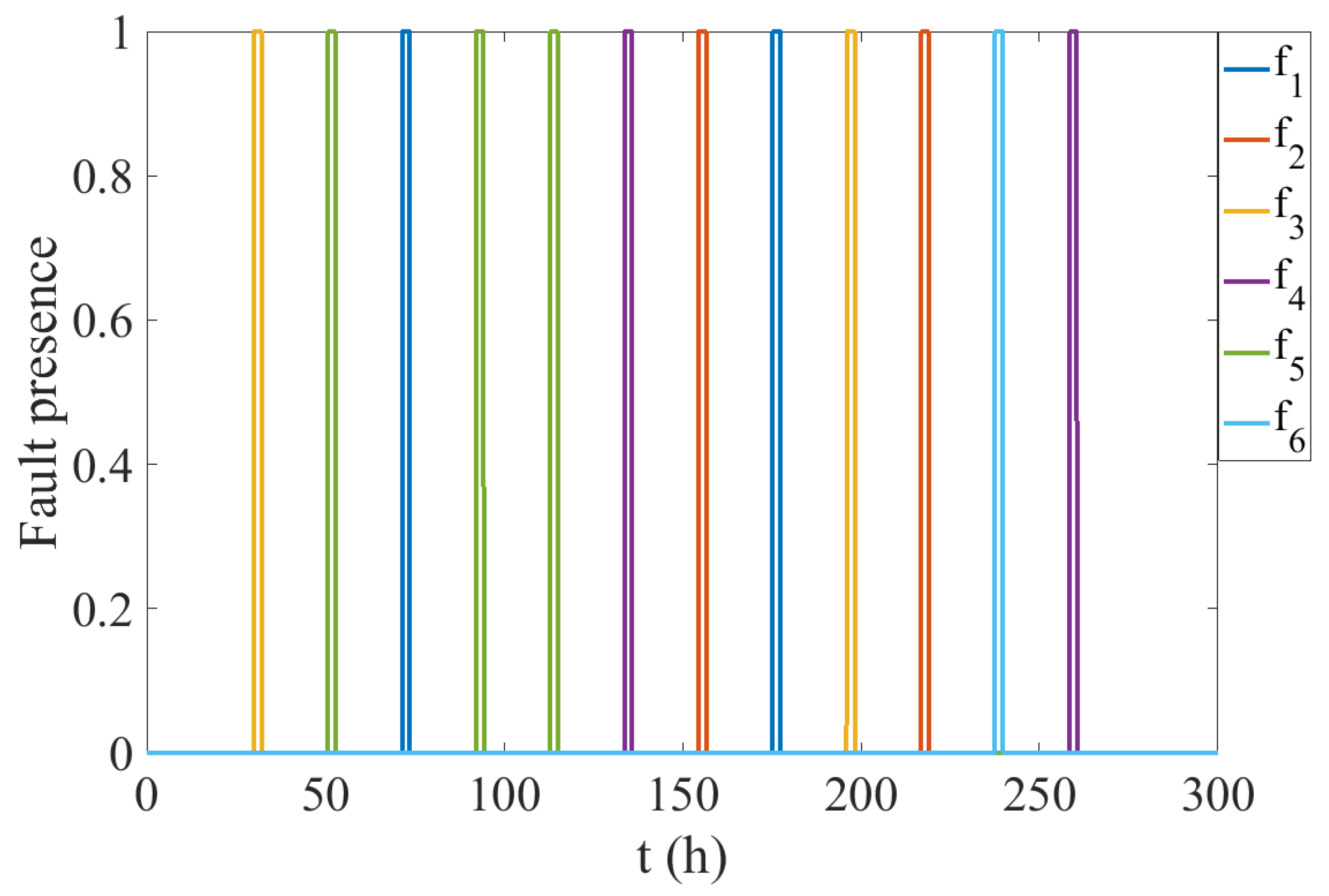
4.3. Fault Detection and Isolation

In the following, we will showcase the performance of the algorithm in its Phase II which includes the detection and isolation of fault signals from an observed data set. For demonstration purposes, we will portray the steps of the detection algorithm on a data set where 12 random faults were observed in a time span of 300 h. Parallel to faults known, changes within the input variables were also introduced. This allowed the observation of the system’s FDI capabilities under changing operation regimes. The fault signals present as well as the known input changes for the observation are shown in Figure 8.

The responses of the tank level within the system have been observed for both the know input changes and the unknown fault presences. The data pertaining to the level changes within the tank was assumed to be polluted with Gaussian noise with a mean of zero and standard deviation of 0.02. The observed data set was centered around the expected values of process variables in the steady-state operation points of the system. After applying the established DPCA transformation to the data, the dynamic changes within the PC subspace were observed. Response signals of the system as well as the system trajectories within the PC subspace are shown in Figure 9.

The value of the Q-statistic for each data point was calculated. Outliers were identified based on the control limit of the statistic for a confidence value of $\alpha =0.1$, and the trajectories of outliers within the PC subspace were collected. The Q values of the time-series data along with the trajectories of outliers within the normalized PC subspace are displayed in Figure 10. For better comparison, the outlier trajectories for known faults shown in Figure 7 were also displayed within the normalized PC subspace.

The Q values pinpoint prediction errors for the model. Outliers of the statistic that exceed the calculated control limit appear at the same time as the fault signals shown in Figure 8a. Thus, the statistical limit was able to accurately pinpoint the presence of abnormalities within the observed data. After extracting and normalizing the outlier trajectories and plotting them within the normalized PC subspace, it can be seen that albeit polluted with noise, they greatly resemble the trajectories of the established reference faults seen in Figure 10b.

After calculating the Fréchet distance between the points of each outlier and the reference fault trajectories within the normalized PC subspace, a prediction has been made about the nature of identified outliers. The predicted fault types based on the evaluation of trajectory similarity within the normalized PC subspace are displayed as a function of time as binary signals, with a value of zero indicating absence of a specific fault and a value of one indicating a specific fault instance.

After comparing Figure 11 which shows the recognized abnormalities and their predicted root causes with Figure 8a, it can be concluded that the method accurately detected the presence of outliers and categorized them adequately.

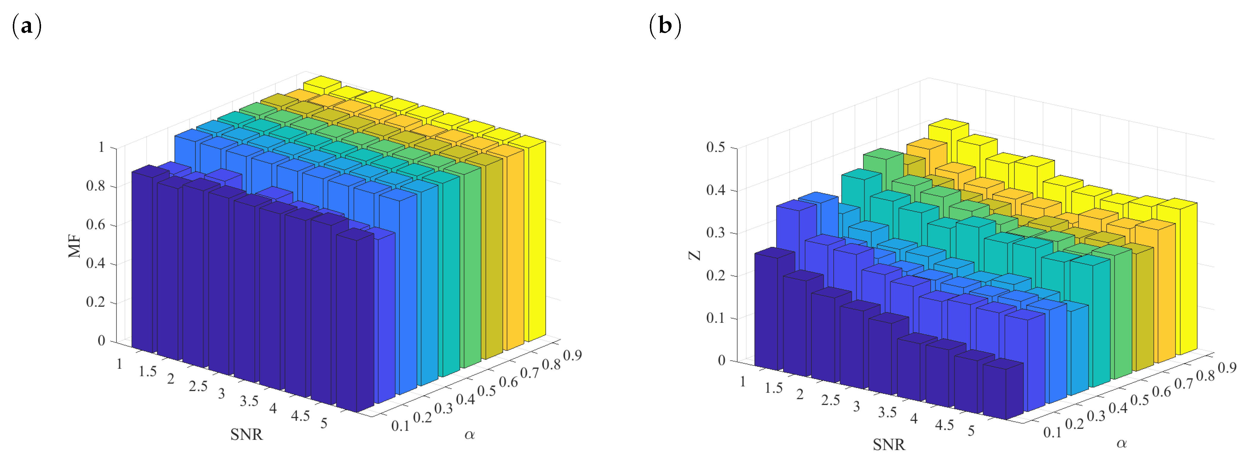
4.4. Performance Metrics of the Method

In order to give measures for characterizing the method, simulations with increased fault numbers were conducted. The presence of 600 randomly generated faults was observed in a time interval of 6000 h.

In the following, the micro-averaged F score $\left(MF\right)$ as well as FAR and MAR metrics of the method will be displayed for different confidence values of statistical testing $\left(\alpha \right)$ and measurement signal-to-noise ratio $\left(SNR\right)$.

The achieved FAR and MAR metrics as functions of $\alpha$ and $SNR$ are displayed in Figure 12.

Figure 12a shows that FAR decreases as both $SNR$ and $\alpha$ increase. This is expected since false alarms are due to the presence of process measurement noise as well as due to strict restrictions on the acceptable range of process variables. The decrease of the noise variance compared to the fault signals results in better decoupling of noise and actual faults. Additionally, with the increase of $\alpha$, the acceptable range of the Q-values increases, resulting in fewer false alarms due to small deviations from the expected process variables via measurement noise.

In contrast, Figure 12b shows that MAR increases as a function of $\alpha$ and is mostly unaffected by $SNR$. This is expected since noise does not prevent recognition of fault signals if the statistical limits are adequate. On the other hand, with increasing value of $\alpha$, the acceptable deviation from the process variables under normal operating conditions also increases. This results in smaller faults going unrecognized as their respective Q-values fall under the control limit.

Figure 13 displays the average of FAR and MAR denoted as Z as well as the isolation capabilities of the classifier expressed as the value of $MF$ for the observed cases.

Figure 13a shows the $MF$ value for the possible observation points. Based on the results, the classifier has good precision and recall for all fault classes under varying operating conditions, resulting in high $MF$ scores close to one. The isolation capabilites of the method weaken, however, in the presence of low $\alpha$ values. This is to be expected since with low values of $\alpha$ many small-scale faults may be recognized, but the trajectories of the small fault signals within the PC subspace will be highly distorted by the presence of noise resulting in higher misclassification rates. By increasing $\alpha$, small-scale faults are filtered out, and only fault signals remain in which the fault signal’s trajectory within the PC subspace stays dominant compared to the noise resulting in strong isolation capabilities.

Figure 13b shows that both high and low values of $\alpha$ are generally unfavourable due to the high value of FAR and MAR, respectively. However, the optimum cut-off value for the control limit significantly depends on the $SNR$ of the observed data. Nonetheless, in the observed system, the measure based on the Q-statistic used for the PC values could provide reliable detection through proper choice of $\alpha$.

5. Discussion

In this work, a proposed FDI method was studied that utilized DPCA for feature extraction from a process to achieve FD combined with the Fréchet distance metric for isolation purposes. The motivation behind the research was to provide a diagnostic method with little computational complexity and computational load that still provides robust and sensitive FDI capabilities.

As noted in many review articles concerning FDI, while extremely robust, diagnostic techniques that utilize explicit mathematical models of the process are often burdened by great complexity, modeling uncertainties and restricted applications [1]. On the other hand, data-based methods have become influential due to the absence of a need for an explicit process model which makes their formulation much simpler. While not suffering from explicit difficulty due to complex model structures, many data-based machine learning techniques for FDI have issues for online implementation and identification due to high computational cost and low-quality training data [18]. This is especially prominent for neural networks which have become a strong focus for academic research concerning FDI. As noted by Khoukhi and Khalid, computational complexity is a major issue for many FDI strategies based on supervised learning algorithms that limit their application in certain areas [41]. In contrast, the proposed method utilizes DPCA which is a data transformation method with low computational cost. Due to the dimensionality reduction aspect of DPC,A the computational cost of the subsequent Fréchet-distance-based fault isolation scheme can also be lowered.

In this work, the method showcased good robustness and sensitivity as well for the supervision of a nonlinear system. This was explored by investigating the FAR and MAR metrics as well as the MF-score for the proposed scheme under a wide range of conditions with simulated operating time of 6000 h in the presence of 600 process faults with varying magnitudes. The technique displayed strong detection and isolation capabilities even under extreme conditions of signal-to-noise ratio of 1 with an average FAR and MAR of 0.2 with proper tuning of the parameter for statistical confidence level $\alpha$ as seen in Figure 12. This was accompanied by an MF score greater than 0.8, showing that the isolation capabilities of the system did not deteriorate even in the presence of extreme noise signals which could be observed in Figure 13.

An additional strength of the method lies in the ability to extend it for a variety of methods derived from PCA capable of handling various issues which would be difficult for conventional ML techniques, such as missing data during training or varying scales of data (MSPCA). The possibility of extending the method for nonlinear PCA variants is also promising for describing a wide range of dynamic processes. With the proper adjustments, the method may also find a promising place in detecting the time evolution of faults in not just chemical systems but different material structures, human health, etc. These applications are not uncommon, as seen in the works of Janeliukstis et al. who utilized a supervised learning scheme for defect localisation in carbon composite structures [42]. Similar to the presented method, they utilized a classification algorithm for the localisation of impacts and stress within the material based on strain values. Oliveira et al. used convolutional neural networks as well as PCA for segmentation and analysis of images of carbon-fibre-reinforced plastic structures. In their work, they trained a neural network based on optical lock-in termography for the recognition of faults within the carbon fibre reinforced plastic and assessing structural integrity. They compared their method with several schemes, ones based on PCA as well [43]. By considering the use of the proposed scheme, the time evolution of structural faults may be predicted and recognized early on. This could highlight the possibility of also utilizing the technique as a reliable tool for predictive maintenance.

As a demerit, it must also be noted that the technique may suffer from the same issues as PCA, such as mischaracterization of the process due to the presence of outliers or a wrong choice of principal components, which all impede FDI capabilities. The employed statistical test for FD is also a critical issue as is the choice of the statistical confidence level $\alpha$ due to the possibility of high FAR and MAR.

In order to compile the possible merits and demerits of the proposed method,

Table 2. Comparison of the proposed method with other popular FDI approaches (+ indicating positive, − indicating negative qualities) [1,7,18].

Consideration	Model-Based Techniques	Neural Networks	Proposed Method
Complexity	Requires deep mathematical and system knowledge to implement (−)	Easy implementation (+)	Easy implementation (+)
Requirements	Exact process model (−)	Abundance of reliable process data (−)	Abundance of reliable process data (−)
Adaptability to new faults	Easy adaptability (+)	Requires additional training to identify new fault classes (−)	Easy addition of new faults to the data base after fault occurrence (+)
Computational load	Low computational cost (+)	Depending on the network structure computational cost may be high (−)	Low computational cost (+)
Design procedure	Straightforward & simple (+)	Great consideration has to be given to determine the optimal network structure (−)	Straightforward and simple (+)
Robustness against noise and disturbances	Robustness may be an issue for nonlinear systems (−)	Great robustness depending on the network structure (+)	Robustness is easy to adjust through the use of nonlinear PCA (+)
Sensitivity to faults	Great sensitivity (+)	Great sensitivity (+)	Sensitivity may be an issue based on the utilized statistic (−)

contains a comparison of the proposed technique and standard FDI techniques found in literary sources based on general considerations for the evaluation of FDI methods. To summarize, the proposed technique presents a flexible and low computational cost alternative for FDI with proper sensitivity and robustness. Since the PCA technique may be extended to nonlinear approximations as well, handling of nonlinear systems is also possible. An issue may be the noise sensitivity of the method depending on the utilized statistics for the FD procedure; however, this may be circumvented through the proper optimization of statistic confidence thresholds.

6. Conclusions

In this work, an FDI scheme was introduced which utilized DPCA to obtain a reduced set of variables from an observed system under normal system behaviour and establish statistical control limits for the detection of abnormalities. Knowledge of characteristic faults within the system has been utilized to establish a fault library and develop an isolation method which compares trajectories of registered faults with those found in the library. The discrete Fréchet distance metric was utilized to analyze system behaviour and isolate recognized fault instances. To the best of the authors knowledge, the combination of these two techniques is a novel contribution to the FDI framework which due to its data-based nature fits well into the modern process control and diagnostic practice. Findings within the paper indicate that the method incorporates robust and sensitive FDI abilities in addition to low computational cost. The FDI capabilities of the proposed algorithm have been validated using data gathered from the first principle model of a three-tank benchmark system. Based on the results, the method has strong classification capabilities with a macro-averaged F score of at least 0.8 for investigated cases. FAR and MAR could be optimized based on the confidence level of statistical testing to reach an average of only 0.1. Possible future directions of the proposed research include using nonlinear PCA techniques to better characterize system behaviour and fault isolation conducted with other trajectory similarity metrics to optimize computational cost and FDI capability of the method.

References

1. Venkatasubramanian, V.; Rengaswamy, R.; Yin, K.; Kavuri, S.N. A review of process fault detection and diagnosis: Part I: Quantitative model-based methods. Comput. Chem. Eng. 2003, 27, 293–311. [Google Scholar]
2. De, S.; Shanmugasundaram, D.; Singh, S.; Banerjee, N.; Soni, K.; Galgalekar, R. Chronic respiratory morbidity in the Bhopal gas disaster cohorts: A time-trend analysis of cross-sectional data (1986–2016). Public Health 2020, 186, 20–27. [Google Scholar]
3. Kalantarnia, M.; Khan, F.; Hawboldt, K. Modelling of BP Texas City refinery accident using dynamic risk assessment approach. Process Saf. Environ. Prot. 2010, 88, 191–199. [Google Scholar]
4. Laboureur, D.M.; Han, Z.; Harding, B.Z.; Pineda, A.; Pittman, W.C.; Rosas, C.; Jiang, J.; Mannan, M.S. Case study and lessons learned from the ammonium nitrate explosion at the West Fertilizer facility. J. Hazard. Mater. 2016, 308, 164–172. [Google Scholar]
5. Chien, S.S.; Chang, Y.T. Explosion, subterranean infrastructure and the elemental of earth in the contemporary city: The case of Kaohsiung, Taiwan. Geoforum 2021, 127, 424–434. [Google Scholar]
6. Sivaraman, S.; Tauseef, S.; Siddiqui, N. Investigative and probabilistic perspective of the accidental release of styrene: A case study in Vizag, India. Process Saf. Environ. Prot. 2022, 158, 55–69. [Google Scholar]
7. Park, Y.J.; Fan, S.K.S.; Hsu, C.Y. A review on fault detection and process diagnostics in industrial processes. Processes 2020, 8, 1123. [Google Scholar]
8. Zhong, M.; Xue, T.; Ding, S.X. A survey on model-based fault diagnosis for linear discrete time-varying systems. Neurocomputing 2018, 306, 51–60. [Google Scholar]
9. Li, Y.; Karimi, H.R.; Ahn, C.K.; Xu, Y.; Zhao, D. Optimal residual generation for fault detection in linear discrete time-varying systems with uncertain observations. J. Frankl. Inst. 2018, 355, 3330–3353. [Google Scholar]
10. Nemati, F.; Hamami, S.M.S.; Zemouche, A. A nonlinear observer-based approach to fault detection, isolation and estimation for satellite formation flight application. Automatica 2019, 107, 474–482. [Google Scholar]
11. Wang, P.; Zou, P.; Yu, C.; Sun, J. Distributed fault detection and isolation for uncertain linear discrete time-varying heterogeneous multi-agent systems. Inf. Sci. 2021, 579, 483–507. [Google Scholar]
12. Wu, Y.; Zhao, D.; Liu, S.; Li, Y. Fault detection for linear discrete time-varying systems with multiplicative noise based on parity space method. ISA Trans. 2022, 121, 156–170. [Google Scholar]
13. Zhang, W.; Peng, G.; Li, C.; Chen, Y.; Zhang, Z. A new deep learning model for fault diagnosis with good anti-noise and domain adaptation ability on raw vibration signals. Sensors 2017, 17, 425. [Google Scholar]
14. Toma, R.N.; Prosvirin, A.E.; Kim, J.M. Bearing fault diagnosis of induction motors using a genetic algorithm and machine learning classifiers. Sensors 2020, 20, 1884. [Google Scholar]
15. Lee, C.Y.; Cheng, Y.H. Motor fault detection using wavelet transform and improved PSO-BP neural network. Processes 2020, 8, 1322. [Google Scholar]
16. Ait-Izem, T.; Harkat, M.F.; Djeghaba, M.; Kratz, F. On the application of interval PCA to process monitoring: A robust strategy for sensor FDI with new efficient control statistics. J. Process Control. 2018, 63, 29–46. [Google Scholar]
17. Vanhatalo, E.; Kulahci, M.; Bergquist, B. On the structure of dynamic principal component analysis used in statistical process monitoring. Chemom. Intell. Lab. Syst. 2017, 167, 1–11. [Google Scholar]
18. Venkatasubramanian, V.; Rengaswamy, R.; Kavuri, S.N.; Yin, K. A review of process fault detection and diagnosis: Part III: Process history based methods. Comput. Chem. Eng. 2003, 27, 327–346. [Google Scholar]
19. Bakdi, A.; Kouadri, A. A new adaptive PCA based thresholding scheme for fault detection in complex systems. Chemom. Intell. Lab. Syst. 2017, 162, 83–93. [Google Scholar]
20. Kramer, M.A. Nonlinear principal component analysis using autoassociative neural networks. AIChE J. 1991, 37, 233–243. [Google Scholar]
21. Mansouri, M.; Nounou, M.; Nounou, H.; Karim, N. Kernel PCA-based GLRT for nonlinear fault detection of chemical processes. J. Loss Prev. Process Ind. 2016, 40, 334–347. [Google Scholar]
22. Li, W.; Yue, H.H.; Valle-Cervantes, S.; Qin, S.J. Recursive PCA for adaptive process monitoring. J. Process Control. 2000, 10, 471–486. [Google Scholar]
23. Ammiche, M.; Kouadri, A.; Bensmail, A. A modified moving window dynamic PCA with fuzzy logic filter and application to fault detection. Chemom. Intell. Lab. Syst. 2018, 177, 100–113. [Google Scholar]
24. Ku, W.; Storer, R.H.; Georgakis, C. Disturbance detection and isolation by dynamic principal component analysis. Chemom. Intell. Lab. Syst. 1995, 30, 179–196. [Google Scholar]
25. Rato, T.J.; Reis, M.S. Fault detection in the Tennessee Eastman benchmark process using dynamic principal components analysis based on decorrelated residuals (DPCA-DR). Chemom. Intell. Lab. Syst. 2013, 125, 101–108. [Google Scholar]
26. Huang, S.; Yang, X.; Wang, L.; Chen, W.; Zhang, F.; Dong, D. Two-stage turnout fault diagnosis based on similarity function and fuzzy c-means. Adv. Mech. Eng. 2018, 10, 1687814018811402. [Google Scholar]
27. Bounoua, W.; Bakdi, A. Fault detection and diagnosis of nonlinear dynamical processes through correlation dimension and fractal analysis based dynamic kernel PCA. Chem. Eng. Sci. 2021, 229, 116099. [Google Scholar]
28. Stanimirova, I.; Daszykowski, M.; Walczak, B. Dealing with missing values and outliers in principal component analysis. Talanta 2007, 72, 172–178. [Google Scholar]
29. Dray, S.; Josse, J. Principal component analysis with missing values: A comparative survey of methods. Plant Ecol. 2015, 216, 657–667. [Google Scholar]
30. Kwon, J.; Oh, H.S.; Lim, Y. Dynamic principal component analysis with missing values. J. Appl. Stat. 2020, 47, 1957–1969. [Google Scholar]
31. Bakshi, B.R. Multiscale PCA with application to multivariate statistical process monitoring. AIChE J. 1998, 44, 1596–1610. [Google Scholar]
32. Misra, M.; Yue, H.H.; Qin, S.J.; Ling, C. Multivariate process monitoring and fault diagnosis by multi-scale PCA. Comput. Chem. Eng. 2002, 26, 1281–1293. [Google Scholar]
33. Sophian, A.; Tian, G.Y.; Taylor, D.; Rudlin, J. A feature extraction technique based on principal component analysis for pulsed Eddy current NDT. NDT Int. 2003, 36, 37–41. [Google Scholar]
34. Lau, C.; Ghosh, K.; Hussain, M.A.; Hassan, C.C. Fault diagnosis of Tennessee Eastman process with multi-scale PCA and ANFIS. Chemom. Intell. Lab. Syst. 2013, 120, 1–14. [Google Scholar]
35. Weng, H.; Wang, S.; Wan, Y.; Lin, X.; Li, Z.; Huang, J. Discrete Fréchet distance algorithm based criterion of transformer differential protection with the immunity to saturation of current transformer. Int. J. Electr. Power Energy Syst. 2020, 115, 105449. [Google Scholar]
36. Jackson, J.E.; Mudholkar, G.S. Control procedures for residuals associated with principal component analysis. Technometrics 1979, 21, 341–349. [Google Scholar]
37. Eiter, T.; Mannila, H. Computing Discrete Fréchet Distance; Technical Report CD-TR 94/64; Christian Doppler Laboratory for Expert Systems: Vienna, Austria, 1994. [Google Scholar]
38. Theilliol, D.; Noura, H.; Ponsart, J.C. Fault diagnosis and accommodation of a three-tank system based on analytical redundancy. ISA Trans. 2002, 41, 365–382. [Google Scholar]
39. Li, Y.; Cao, W.; Hu, W.; Xiong, Y.; Wu, M. Incipient fault detection for geological drilling processes using multivariate generalized Gaussian distributions and Kullback–Leibler divergence. Control. Eng. Pract. 2021, 117, 104937. [Google Scholar]
40. Cuadros-Rodríguez, L.; Pérez-Castaño, E.; Ruiz-Samblás, C. Quality performance metrics in multivariate classification methods for qualitative analysis. TrAC Trends Anal. Chem. 2016, 80, 612–624. [Google Scholar]
41. Khoukhi, A.; Khalid, M.H. Hybrid computing techniques for fault detection and isolation, a review. Comput. Electr. Eng. 2015, 43, 17–32. [Google Scholar]
42. Janeliukstis, R.; Rucevskis, S.; Chate, A. Condition monitoring with defect localisation in a two-dimensional structure based on linear discriminant and nearest neighbour classification of strain features. Nondestruct. Test. Eval. 2020, 35, 48–72. [Google Scholar]
43. Oliveira, B.; Seibert, A.; Borges, V.; Albertazzi, A.; Schmitt, R. Employing a U-net convolutional neural network for segmenting impact damages in optical lock-in thermography images of CFRP plates. Nondestruct. Test. Eval. 2021, 36, 440–458. [Google Scholar]
Figure 1. The investigated three-tank benchmark system [38].
Processes 10 02409 g001
Figure 2. Change of level within the tank in the investigated steady-state [38].
Processes 10 02409 g002
Figure 3. (a) Input signals of the three-tank system over the investigated time window; (b) system responses to the inputs over the observed time window.
Processes 10 02409 g003
Figure 4. (a) Scree plot of the DPCA transformation; (b) cumulative variance retained within the PCs.
Processes 10 02409 g004
Figure 5. (a) Representation of the observed data in the 2D PC subspace; (b) representation of the observed data in the 3D PC subspace.
Processes 10 02409 g005
Figure 6. (a) Fault signals within the system; (b) fault responses of the unit.
Processes 10 02409 g006
Figure 7. Normalized trajectories of isolated faults within the PC subspace.
Processes 10 02409 g007
Figure 8. (a) Fault signals observed for validation; (b) changes within the inputs of the system.
Processes 10 02409 g008
Figure 9. (a) Fault responses observed within the validation data set; (b) system dynamics as observed within the PC subspace.
Processes 10 02409 g009
Figure 10. (a) Value of Q for the observed data as a function of time; (b) outlier data within the PC subspace along with normalized responses of known faults.
Processes 10 02409 g010
Figure 11. Predicted fault instances for the validation data set.
Processes 10 02409 g011
Figure 12. (a) FAR as a function of α and S N R ; (b) MAR as a function of α and S N R , with different colored bars responding to a fixed α value.
Processes 10 02409 g012
Figure 13. (a) MF as a function of α and S N R ; (b) Z as a function of α and S N R , with different colored bars responding to a fixed α value.
Processes 10 02409 g013