Article

Distribution Network Fault-Line Selection Method Based on MICEEMDAN–Recurrence Plot–Yolov5

1
School of Electrical and Electronic Engineering, North China Electric Power University, Baoding 071003, China
2
School of Electrical and Control Engineering, North China University of Technology, Beijing 100144, China
*
Authors to whom correspondence should be addressed.
Processes 2022, 10(10), 2127; https://doi.org/10.3390/pr10102127
Submission received: 14 September 2022 / Revised: 11 October 2022 / Accepted: 15 October 2022 / Published: 19 October 2022

Abstract

:
Distribution system fault signals contain severe noise components. In order to solve the problem of distribution network fault-line selection, a fault-line selection method based on modifying the Improved Complete Ensemble Empirical Mode Decomposition Adaptive Noise (MICEEMDAN) algorithm, Recurrence Plot, and Yolov5 network is proposed. First, ICEEMDAN is optimized using multi-scale weighted permutation entropy (MWPE). MICEEMDAN can decompose an electrical signal into a series of intrinsic mode functions (IMFs). Recurrence Plot transformation of all IMFs, obtained from decomposition and stitching from top to bottom, realizes the conversion of 1D time series to 2D images. Then, the recurrence maps obtained from all lines in the distribution network are stitched to obtain the distribution network recurrence map, realizing the mining of the fault-signal features of the whole distribution network. Finally, the Yolov5 network is used to mine the fault features of the recurrence map of the distribution network autonomously to realize the fault-line selection. The experiments show that the method has a good noise immunity and 99.98% fault-selection accuracy, which can effectively complete the distribution network fault selection.

1. Introduction

The distribution network topology is becoming increasingly complex, and the occurrence of faults is unavoidable. If faults are not recovered in time, it will impact users’ electricity safety. Therefore, it is essential to remove faults in time to ensure the safe and stable operation of the power system [1]. Eighty percent of the faults in medium- and low-voltage distribution networks are caused by single-phase grounding, and fault-line selection is a crucial link in distribution network fault recovery [2]. In recent years, fault-line selection algorithms have received much attention. However, these algorithms are easily affected by neutral grounding methods, transition resistance, and other factors, which make the fault-line selection algorithm for distribution networks have certain limitations [3]. Therefore, studying a more general fault-line selection algorithm for distribution networks is vital.
Currently, there are three main methods of fault-line selection: passive line selection, active line selection, and integrated line selection [4]. The passive line-selection method mainly uses signal characteristics for line selection, including the steady-state component method, transient component method, traveling wave component method, etc. [5]. The active line-selection method mainly uses a sudden change signal or injection signal to achieve fault-line selection, including the small disturbance method, signal injection method, residual flow increment method, etc. [6]. The integrated line-selection method is a combination of the line-selection methods, using more than two different principles, including the use of artificial intelligence and other algorithms, for fault-wire selection [7].
The authors in [8] decomposed the zero-sequence conductance to detect faulty feeders by comparing the spectral characteristics of the calculated zero-sequence conductance. However, different grounding types, line parameters, transition resistances, fault locations, and other factors can lead to different spectral characteristics, making the detection strategy based on spectral fault characteristics ineffective. Reference [9] proposed a method for fault-line selection based on the correlation coefficient of phase current fault component waveforms. However, its actual line-selection accuracy is unsatisfactory due to the virtual environment’s load fluctuation. In [10], the authors use the intrinsic mode energy of the phase current fault component to select the line, but its fault rate is higher for different fault initial phase angles. Reference [11] uses a projection relationship between the line current and the neutral branch current in the same direction to select the line which is not affected by the transition resistance. However, the error is more significant in practical applications because the amplitude and phase information must be used simultaneously. The authors of [12] proposed a method for line selection by extracting the amplitude coefficients of the high-frequency components of the line’s three-phase voltage through a discrete wavelet transform. However, the accuracy of this method for line selection is low in the case of high-resistance grounding, and therefore the applicability is poor. In [13], fault-line selection is performed by comparing the zero sequence currents’ magnitude, polarity, and energy value. However, this method is unavailable when grounding the neutral point via the arc extinguishing coil. The authors of [14] proposed a fault-line selection method based on a chaotic system, which is not affected by fault type, transition resistance, etc. However, since the chaotic system is susceptible to abnormal signals, and the actual distribution network contains many noisy signals, inputting the signals directly into the chaotic system will cause misclassification, and the system’s robustness is poor.
In recent years, artificial intelligence algorithms have developed rapidly, with the advantages of fast processing speed and high fault tolerance. Applying AI algorithms to distribution network fault diagnosis is a significant trend for future development [15]. Deep learning, as a method to achieve artificial intelligence, can autonomously mine the feature information of the input quantity and has superior performance in the field of image recognition and classification. Scholars have used the power signal features of distribution networks as the input of neural networks for fault-line selection, but the advantages of deep learning in image recognition have not been fully utilized.
The authors of [16] constructed a switching and evaluation function to convert the line-selection problem into a Traveling Salesman Problem (TSP). It performs a global search for distribution network faults by improving the ant colony algorithm, which improves the efficiency of the line selection to a certain extent. However, it is easy to fall into a local optimum. Reference [17] proposes a combination of traveling wave and support vector machine methods for fault-line selection, but the accuracy is poor in warhead calibration. The authors in [18] use wavelet transform to capture the amount of current feature variation and use artificial neural networks for fault-line selection. However, traditional neural networks suffer from overfitting and slow convergence during training and cannot fully use the data feature information. In [19], PMU is used to measure the power at each node of the distribution network synchronously, using DBN networks for training models for fault selection, although performing poorly in the case of high-resistance grounding. Reference [20] achieves fault-line selection by superimposing zero-sequence currents to fuse fault features and using entire convolutional networks for feature extraction. However, excessive superimposition of zero-sequence currents for complex distribution networks can cause fault features to be obscured, resulting in features that cannot be extracted accurately, so the method has some limitations. Reference [21] proposed a fault-line selection method based on variational modal decomposition (VMD) and convolutional neural network (CNN), which decomposes the electrical signal by variational modal decomposition, and then up-dimensionalize the electrical signal into an image by the compression coding method, using a convolutional network for classification, which has a high recognition accuracy and is robust. However, it ignores the physical connection between the distribution and neural networks. There is a large amount of redundancy in the input.
This paper proposes a distribution network fault-line selection method to address the above problems based on an improved ICEEMDAN–Recurrence Plot–Yolov5 network. The noise components in the intrinsic modal functions (IMFs) obtained from ICEEMDAN decomposition are eliminated using multi-scale weighted permutation entropy (MWPE). Then the noisy signals are removed by EMD decomposition. The decomposed IMFs are arranged from high to low frequencies. The MICEEMDAN algorithm can effectively reduce noise and suppress the appearance of modal confusion and pseudo-components. The Recurrence Plot algorithm converts the decomposed 1D signals into 2D images and enhances the invisible information of the 1D signals. The Recurrence Plot is stitched to construct a Recurrence Plot of the distribution network, which reduces the redundancy of the training data set and facilitates in-depth learning training. The Yolov5 network is used to train the data set, and the CA attention mechanism is added to speed up the training convergence and improve the accuracy rate. The model obtained from the training can be used to realize distribution network fault-line selection. The method achieves the extraction of fault features and line selection in a data-driven manner, with good accuracy and robustness.
This paper focuses on the distribution network fault feature extraction and autonomous mining problems, and the main work is summarized as follows.
(1) Improvement of ICEEMDAN by using MWPE; the improved method can effectively suppress the appearance of modal confusion and pseudo-components.
(2) The Recurrence Plot algorithm is used to convert a one-dimensional time series into two-dimensional images, fully exploit the minute features in the one-dimensional signal, and stitch the Recurrence Plot to reduce the input redundancy of the neural network, which is conducive to improving the training efficiency.
(3) Adding a CA attention mechanism to the Yolov5 network to speed up the convergence of the model while improving the recognition accuracy.
This paper can be divided into the following sections: Section 1 introduces multi-scale weighted permutation entropy (MWPE); Section 2 introduces the MICEEMDAN algorithm; Section 3 introduces the signal feature-extraction methods, including the Recurrence Plot algorithm and neural network; Section 4 introduces the fault-line selection process; and Section 5 show the experimental results and comparative analysis.

2. Multi-Scale Weighted Permutation Entropy

2.1. Multi-Scale Permutation Entropy

The permutation entropy is a method to detect the randomness and dynamical mutations of the system, which is simple to calculate, noise-resistant, and has good robustness, as only a short time series is required to obtain a stable system characteristic quantity [22]. For a given time series x = {x(i), i = 1, 2, …, n}, the following matrix is obtained after the phase space reconstruction.
[ x ( 1 ) x ( 1 + Γ ) x ( 1 + ( m 1 ) Γ ) x ( 2 ) x ( 2 + Γ ) x ( 2 + ( m 1 ) Γ ) x ( k ) x ( k + Γ ) x ( k + ( m 1 ) Γ ) ]
where m is the embedding dimension and Γ is the delay factor. k = n − (m − 1), and there are k reconstructed components of the matrix, and each reconstructed component has m-dimensional embedding elements.
Arrange the jth component x(j), x(j + Γ), … x(j + (m − 1) Γ), j = 1, 2, …, k of the matrix in ascending order of numerical magnitude to obtain
x ( i + ( j 1 1 ) Γ ) x ( i + ( j 1 1 ) Γ )       x ( i + ( j m 1 ) Γ )
where j1, j2, …, and jm represent the subscript index value of each element in the reconstructed component. If there are two or more equal values in the reconstructed component, such as x(i + (j1 − 1)Γ) = x(i + (j2 − 1)Γ), then it is necessary to sort according to the size of j1 and j2. Satisfying j1 < j2 is sufficient, at which point we have x(i + (j1 − 1)Γ) ≤ x(i + (j2 − 1)Γ).
A sequence of reconstructed symbols can be obtained for each component.
S ( l ) = ( j 1 , j 2 , , j m )
where l = 1, 2, …, k, satisfying km!. Each reconstructed component is an m-dimensional space mapped to an m-dimensional sequence of symbols with a total of m! permutations.
Calculate the probability of each m-dimensional sequence of symbols, P1, P2, …, Pk.
P j = c j sum ( c )
where j = 1, 2, …, k, sum(c) is the sum of the number of occurrences of each ranking result after ranking all reconstructed components, and cj is the number of occurrences of the jth ranking result after ranking all reconstructed components.
According to the definition of Shannon’s entropy, the permutation entropy of the signal sequence x(i) is defined as
PE ( x , m , Γ ) = ( j = 1 k P j ln P j )
The permutation entropy reaches a maximum value of ln(m!) when Pj = 1/m!
In practice, PE is usually normalized.
0 PE = PE ln ( m ! ) 1
A more significant value of the ranking entropy (PE) indicates a more random signal time series and a more complex signal; conversely, a more regular signal sequence and a less complex signal.
The permutation entropy can only detect the complexity and randomness of the time series on a single scale. Moreover, the output time series of complex systems contain characteristic information on multiple scales when the permutation entropy analysis is no longer satisfied [23]. In order to study the multi-scale complexity variation of a time series, multi-scale permutation entropy is proposed.
A time series x = {xi, i = 1, 2, …, N} of length N is coarsely granularized to obtain the coarsely granularized sequence yj(s), whose expression is
y j ( s ) = 1 s i = ( j 1 ) s + 1 j s x i , j = 1 , 2 , , [ N / s ]
where s is the scale factor, s = 1, 2, …; and [N/s] means rounding N/s and calculating the permutation entropy for each coarse-grained sequence yj(s) to obtain the multi-scale permutation entropy. It can be expressed as follows:
MPE ( X , m , Γ , s ) = PE ( y j ( s ) , m , Γ )
Although the multi-scale permutation entropy solves the single problem of permutation entropy at the time scale, the method still has some problems: for example, for the following two reconstructed components.
S ( 1 ) = ( 1 , 2 , 3 , 4 ) S ( 2 ) = ( 1 , 2 , 3 , 10000 )
After sorting them, the results are all (1, 2, 3, 4) with corresponding weights of 1. However, it is evident that the nature of 3 to 4 and 3 to 10,000 of them are very different, leading to the use of multi-scale permutation entropy, and cannot correctly reflect the characteristics of specific mutation signals.

2.2. Multi-Scale Weighted Permutation Entropy

In order to solve the problem that multi-scale permutation entropy cannot correctly reflect the characteristics of specific mutant signals, a multi-scale weighted permutation entropy is proposed. For each reconstructed component, its second-order central moment is calculated as the weight.
Var = 1 m i = 1 m ( j i j ¯ ) 2
where j ¯ = 1 m i = 1 m j i at this point, with Equation (5) becoming
P j = Var j sum ( Var )
where sum(Var) is the sum of the second-order centroids of all reconstructed components, and Varj is the second-order centroid of the reconstructed component corresponding to the jth ranking result after sorting all reconstructed components.

2.3. Parameter Selection and Analysis Comparison

In order to study the influence of embedding dimension and scale factor on the permutation entropy results, multi-scale permutation entropy and multi-scale weighted permutation entropy are used to analyze Gaussian white noise with embedding dimension m = 3, 4, 5, 6, 7 and scale factor s = 1, 2, …, 20, and the experimental results are shown in Figure 1. From Figure 1, it can be seen that when the embedding dimension m is small, the change in the permutation entropy value is not apparent, which cannot reflect the advantage of multi-scale analysis. When the embedding dimension m is large, the internal details of the permutation entropy reconstruction component are homogenized, resulting in a lack of details [24]. After careful consideration, this paper sets the embedding dimension m = 6. When the embedding dimension m = 6 and the scale factor s > 6, the decreasing trend in the permutation entropy is accelerated, which indicates that, at this time, the scale factor s = 5. The delay factor has less influence on the final calculation result of the permutation entropy, and the delay factor is set to Γ = 1. In summary, we set the embedding dimension m = 6, the scale factor s = 5, and the delay factor Γ = 1.
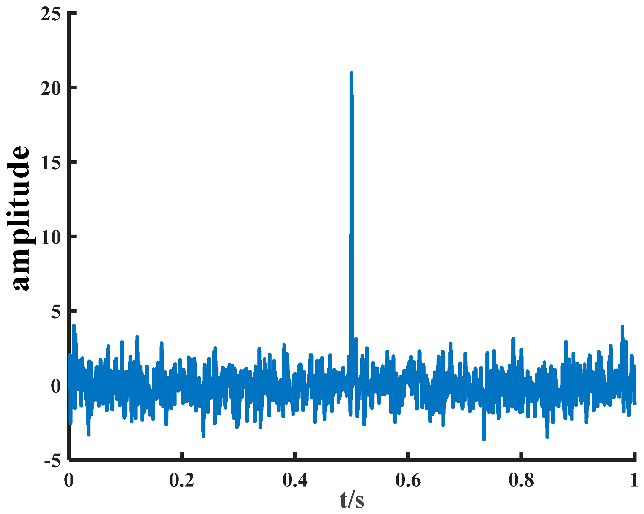
Under the above parameter conditions, a pulse signal is added to the Gaussian white noise to obtain the signal shown in Figure 2, where the sampling frequency is 1000 Hz, and the pulse signal is added at 0.5 s to collect a total of 1000 points.
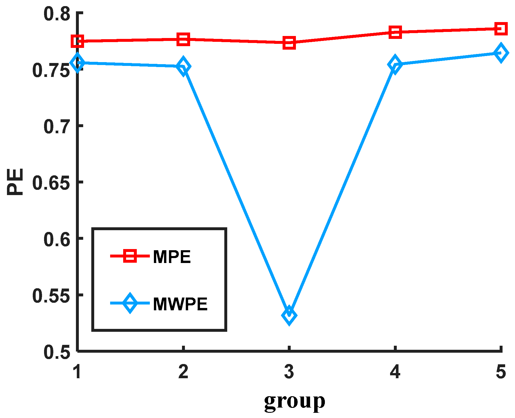
The collected 1000 points were grouped into 200 points in each group. The third group contains the impulse signal, and the entropy values are calculated using multi−scale permutation entropy and multi−scale weighted permutation entropy, respectively. The results are shown in Figure 3.
It is evident from Figure 3 that the entropy value of multi-scale permutation entropy does not change significantly under different groups, which indicates that multi-scale permutation entropy is not sensitive to the mutation signal. In contrast, the entropy value of multi-scale weighted permutation entropy has a significant change in the third group signal, which indicates that it is susceptible to the mutation signal, so multi-scale weighted permutation entropy can better reflect the actual situation of the signal.

2.4. Noise Signal Detection

The entropy values of the white noise, Gaussian white noise, high-frequency sinusoidal signal, fundamental frequency sinusoidal signal, amplitude-modulated signal (AM signal), frequency-modulated signal (FM signal), AM/FM signal, and intermittent signal were calculated by multi-scale permutation entropy and multi-scale weighted permutation entropy, respectively, and the results are shown in Table 1.
It is necessary to give a reference value β to determine whether the signal is noisy or not according to the entropy value of the permutation entropy, and Zheng J et al. concluded through several experiments that it is best to take 0.55~0.6 [25], which is taken as β = 0.6 in this paper. From Table 1, it can be seen that the use of multi-scale permutation entropy will produce false judgments for intermittent signals. This is due to the mutation phenomenon in intermittent signals, and the multi-scale permutation entropy is not sensitive to the mutation phenomenon. The multi-scale weighted permutation entropy is sensitive to the mutation phenomenon, so it will not misjudge the intermittent signal. In summary, multi-scale weighted permutation entropy can complete the detection of noisy signals.

3. MICEEMDAN Signal Decomposition

3.1. ICEEMDAN Signal Decomposition

The ICEEMDAN signal processing method proposed by Colominas et al. [26]. was developed from the Complete Ensemble Empirical Mode Decomposition Adaptive Noise (CEEMDAN) [27]. The improved method differs from CEEMDAN in that Gaussian white noise is added directly during decomposition. However, the Kth IMF component of the white noise is selected after EMD decomposes it. The specific steps are as follows:
(1)
Add Group I white noise to the original signal; i.e.,
x ( i ) = x + β 0 E ( w ( i ) )
where x is the signal to be decomposed; β0 is the intensity factor of the white noise; E(·) denotes the kth order modal component generated by the EMD decomposition; and w(i) is the Gaussian noise.
(2)
The first set of residuals is obtained.
R 1 = ( N ( x ( i ) ) )
where N(·) denotes the local mean value of the generated signal.
(3)
Calculate the first modal component d1 = xR1.
(4)
Continuing with the addition of white noise, the second set of residuals R2 = R1 + β1E(w(i)) is calculated using the local mean decomposition, and the second modal component d2 = R1R2 is defined.
(5)
Calculate the Kth residual RK = (N(RK−1 + βK−1E(w(i)))) and the modal component dK = RK−1RK.
(6)
All modalities and residual numbers are obtained until the end of the computational decomposition.

3.2. ICEEMDAN Signal Decomposition

For the fault signal of the distribution network, the noise will affect the accuracy of the judgment. It is not necessary to use the EMD algorithm to decompose the noisy signal, so the MWPE algorithm can be used in combination with ICEEMDAN to design the MICEEMDAN algorithm for noise filtering of the original signal and decomposition of the signal after noise reduction.
The specific steps of the MICEEMDAN decomposition are as follows.
(1)
The ICEEMDAN decomposition of the original signal I(t) is performed to obtain the K modal components IMF.
(2)
The MWPE calculation is performed for each decomposition of the resulting modal component IMF to obtain the entropy value PE for each modal component.
PE i = MWPE ( IMF i , m , Γ , s )
where, i = 1, 2, …, K.
(3)
When the entropy value obtained from the MWPE calculation is more significant than 0.6, the decomposition signal is considered a noisy signal and is removed from the original signal.
R ( t ) = I ( t ) j = 1 p IMF j
where R(t) is the remaining signal after noise removal and IMFj, j = 1, 2, …, p is the noise component obtained by decomposition.
(4)
The IMF of MICEEMDAN is obtained by decomposing R(t) using EMD, and the results are arranged in high to low frequencies.

3.3. Decomposition of Simulation Signals Using ICEEMDAN and MICEEMDAN

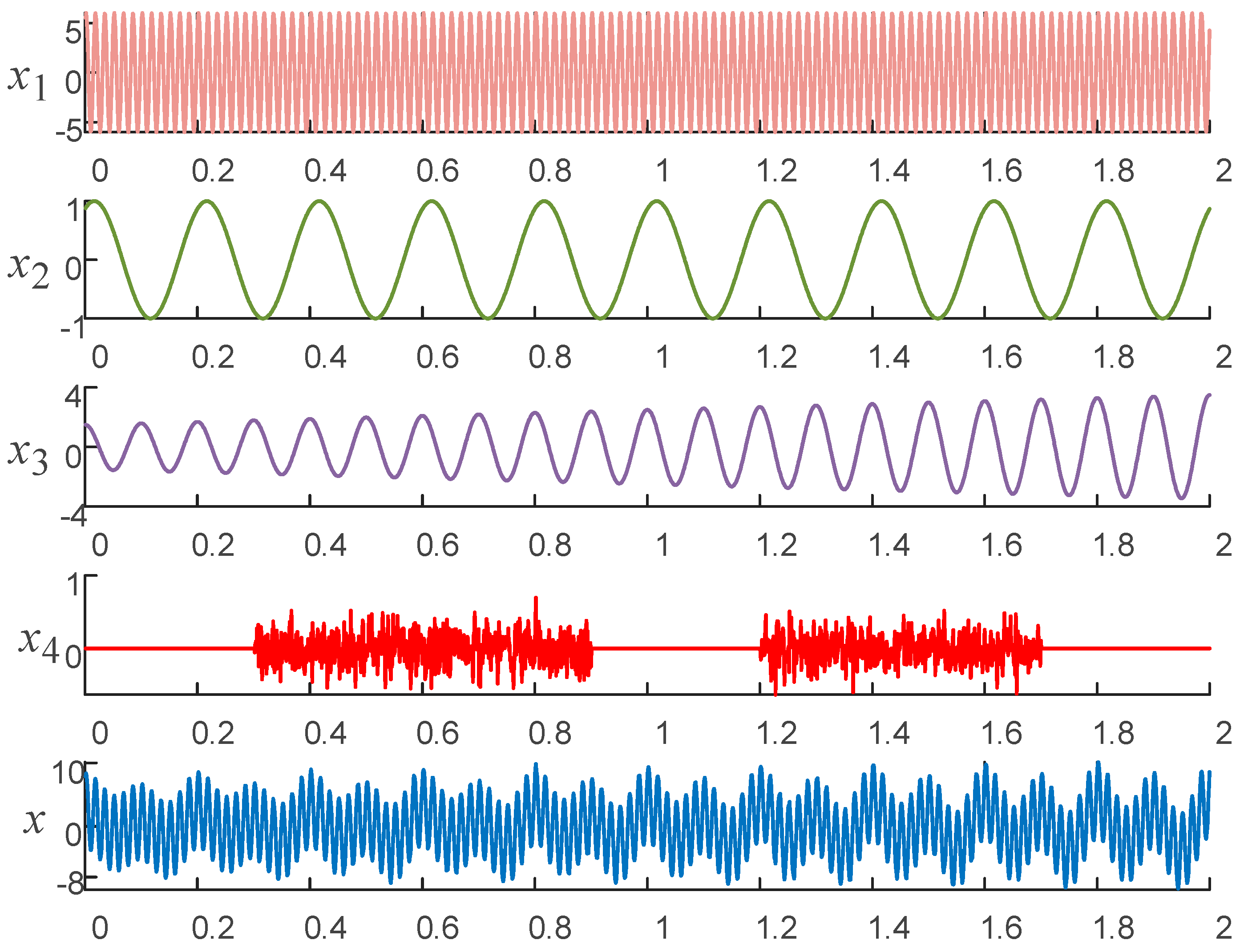
To illustrate the advantages of the MICEEMDAN decomposition, simulation experiments are conducted in this section. The original signal is shown in Equation (16), where (16) consists of x1, x2, x3, and x4, with a sampling frequency of 1000 Hz and a sampling time of 2 s. The original signal is shown in Figure 4.
{ x 1 = 6 sin ( 120 π t + π / 4 ) x 2 = sin ( 10 π t + π / 3 ) x 3 = ( t + 1.5 ) sin ( 20 π t + π / 2 ) x 4 = [ z e r o ( 1 , 300 ) , 0.2 · r a n d n ( 1 , 600 ) ,     z e r o ( 1 , 300 ) , 0.2 · r a n d n ( 1 , 500 ) ,     z e r o ( 1 , 300 ) ] x = x 1 + x 2 + x 3 + x 4
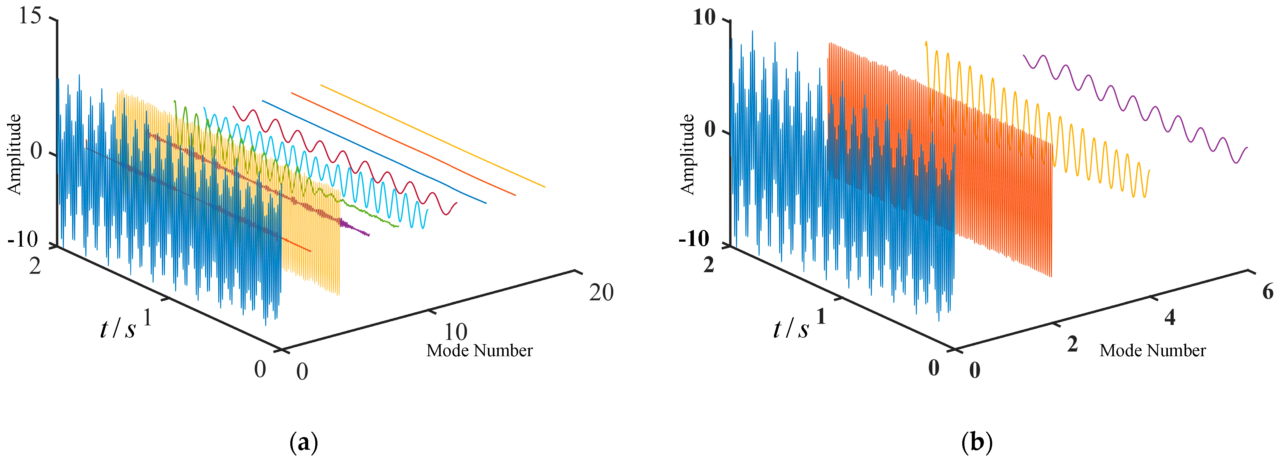
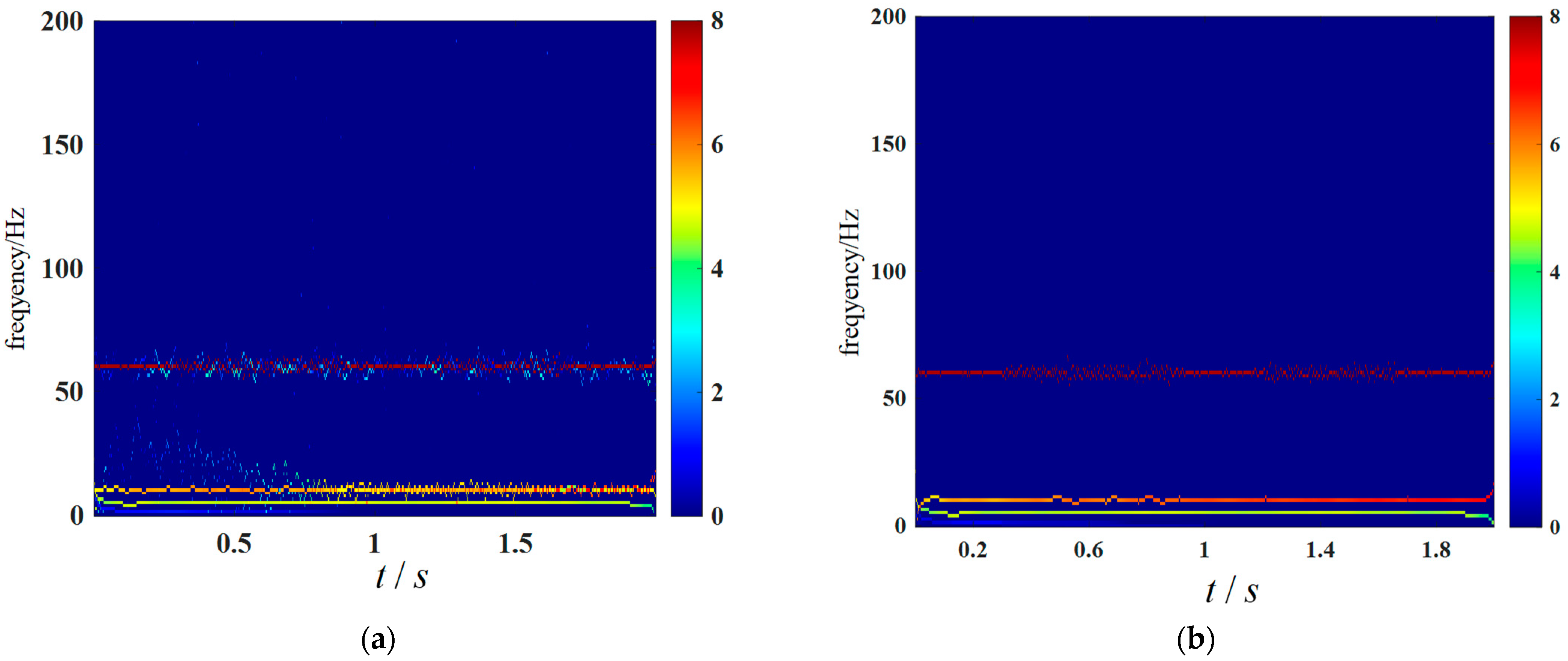
The original signal x is decomposed using ICEEMDAN and MICEEMDAN, respectively, and the decomposed modal components are shown in Figure 5. From Figure 5a, it is evident that the ICEEMDAN algorithm has the problem of modal confusion, the decomposition is not complete, and pseudo-components appear. From Figure 5b, it can be seen that MICEEMDAN has no modal confusion and no pseudo-component, and the noise component is removed.
The concept of the correlation coefficient is introduced to measure the effect of the two decompositions further. The correlation coefficient can be used to analyze the correlation between two signals; the smaller the correlation coefficient, the weaker the correlation between the two signals, and, vice versa, the stronger the correlation between the two signals. It is usually considered that a correlation coefficient greater than 0.8 indicates that the two signals are highly correlated [28]. The correlation coefficients of the two decompositions are shown in Figure 6. The figure shows that in the IMF2 and IMF3, IMF4, and IMF5 obtained by ICEEMDAN decomposition appear modal confusion, and there are pseudo-components. MICEEMDAN can effectively extract x1, x2, and x3 and suppress the modal confusion. The results show that the proposed method in this paper can effectively extract the practical components in the original signal and suppress the modal confusion to some extent.
The Hilbert–Huang spectrum is a standard method for analyzing the time-frequency characteristics of signals [29]. Figure 7 reflects the Hilbert–Huang plots of the two decomposition methods. Figure 7a shows that the ICEEMDAN decomposition extracts the signals at 5 Hz and 10 Hz, but there are many pseudo-components and modal confusion at 60 Hz. From Figure 7b, it can be seen that MICEEMDAN can effectively extract the practical components of the original signal without pseudo-components, and the instantaneous frequency is relatively stable. In summary, the algorithm has a good decomposition effect and overcomes the problems of modal confusion and pseudo-components.

4. Signal Feature Extraction

4.1. Recurrence Plot

A Recurrence Plot is an image representing the distance between trajectories extracted from the original time series and is an essential method for analyzing the periodicity, chaos, and smoothness of time series; it can be used to reveal the internal structure of a time series, giving a priori knowledge of its correlation, informativeness, and predictability. Recurrence Plots are particularly suitable for short time series data and can examine the smoothness and intrinsic similarity of a time series [30]. In this paper, the fault signal of the distribution network is extracted by constructing a Recurrence Plot. The specific steps are as follows.
(1)
MICEEMDAN decomposition of the zero-sequence current signal during a distribution network fault is performed to obtain its modal components IMF1, IMF2
(2)
For a given time series {x(i), i = 1, 2, …, n}, the extracted trajectories are
x i = ( x i , x i + Γ , , x i + ( m 1 ) Γ )
where i = 1, 2, …, n − (m − 1), m is the dimension of the trajectory and Γ is the delay; in this paper, let m = 1, Γ = 1.
(3)
Calculate the distance di,j between any two points on the trajectory.
d i , j = x i x j
(4)
Calculate the recurrence matrix Ri,j.
R i , j = Θ ( ε d i , j )
where ε is the threshold value of the minimum distance. The size chosen in this paper is 15% of the standard deviation of the data, and Θ is the Heaviside function, the expression of which is
Heaviside ( x ) = { 1 x 0 0 x < 0
(5)
The modal components obtained from the decomposition are all Recurrence Plot transformed and stitched from top to bottom.
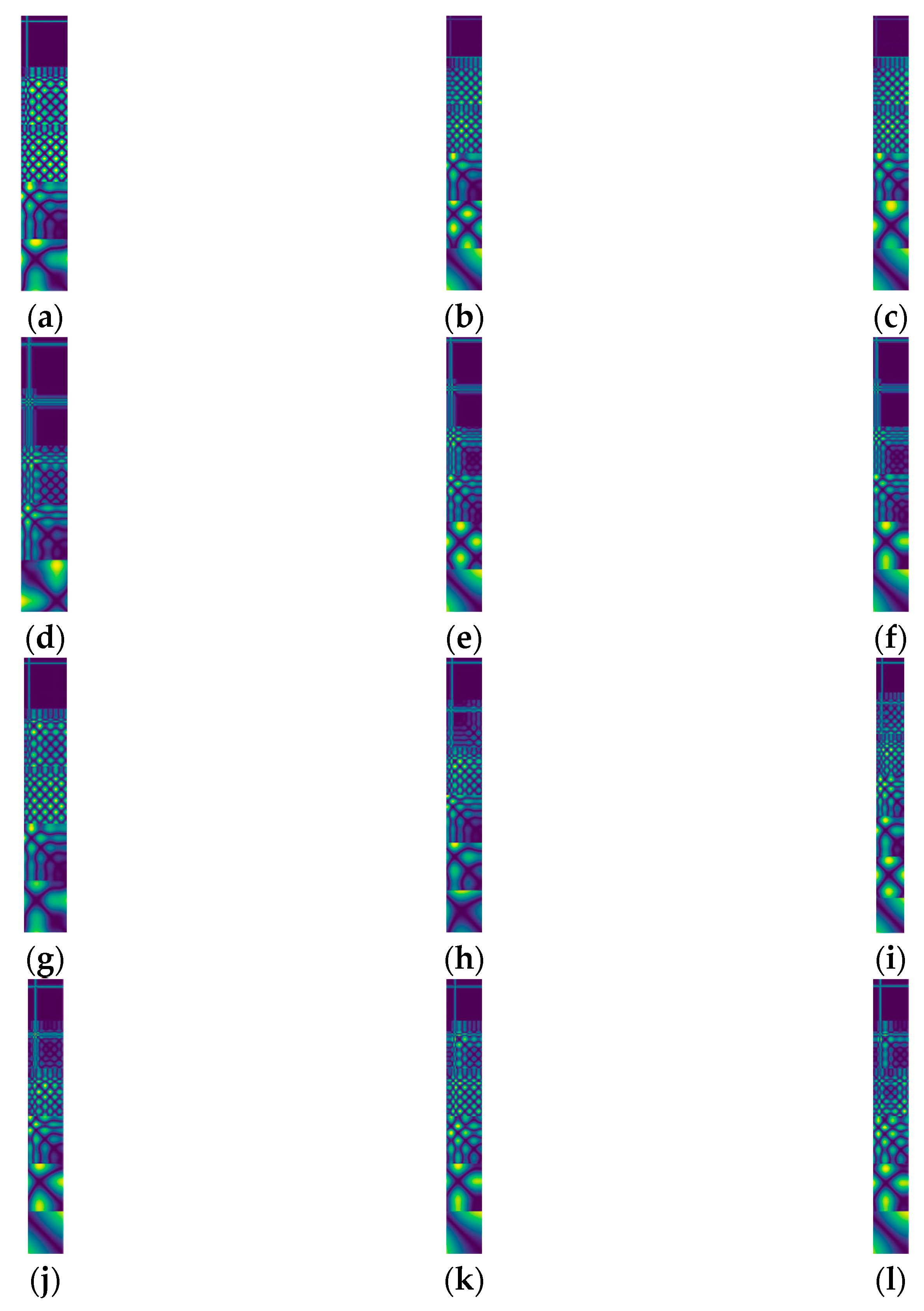
The grounding resistance is 10 Ω, 500 Ω, and 1500 Ω; the grounding phase is the A, B, and C phase; the initial phase angle of the fault is 0°, 60°, and 120°; and the fault distance is 2, 4, and 6 km from the first end of the line. The generated Recurrence Plot is shown in Figure 8. In Figure 8, it can be seen that for different fault types, the Recurrence Plots obtained by the construction have more obvious differences, and the fault characteristics of the distribution network are thoroughly extracted.

4.2. CA Attention Mechanism

This paper introduces the Coordinate Attention (CA) attention mechanism in the feature-extraction process.
The CA attention mechanism module can enhance the expression ability of the network learning features and output a tensor of the same size after transforming any intermediate feature tensor in the network [31]; its module structure is shown in Figure 9. For the input feature map, firstly, average pooling is performed on the width and height to obtain the feature map in both directions; after that, the two feature maps are stitched together and fed into a shared convolution module; then normalization is performed, and a convolution operation with a convolution kernel of 1 × 1 is performed; after that, the attention weights of the feature maps on the height and width are obtained by the sigmoid activation function, respectively. Finally, the weighting calculation is performed on the original feature map, and the feature map with attention weights is finally obtained.
The specific implementation steps are as follows:
(1)
Divide the input feature map into two directions, width and height, and perform global average pooling to obtain the feature maps in both the width and height directions, as shown in Equation (21).
z c h ( h ) = 1 W 0 i W | x c ( h , i ) z c h ( w ) = 1 H 0 j H | x c ( j , w )
(2)
The feature maps in the width and height directions of the obtained global perceptual field are stitched together, after which they are fed into the convolution module with a shared convolution kernel of 1 × 1 to reduce their dimension to the original C/r, where C is the channel number and r is the reduction rate, and then the batch normalized feature map F1 is fed into the Sigmoid activation function to obtain the feature map shaped as 1 × (W + H) × C/r feature map f, as shown in Equation (22).
f = δ ( F 1 ( [ z h , z w ] ) )
(3)
The feature map f is convolved with a convolution kernel of 1 × 1 according to the original height and width to obtain the feature maps Fh and Fw, with the same number of channels as the original one. The attention weights gh for the feature maps in the height and width and gw in the width direction are obtained after the Sigmoid activation function, as shown in Equation (23).
g h = σ ( F h ( f h ) ) g w = σ ( F w ( f w ) )
(4)
After the above calculation, the attention weight gh in the height direction and the attention weight gw in the width direction of the input feature map will be obtained. Finally, the final feature map with attention weights in the width and height directions is obtained by multiplying and weighting the original feature map with the formula shown in (24).
y c ( i , j ) = x c ( i , j ) × g c h ( i ) × g c w ( j )

4.3. Improved Yolov5 Neural Network

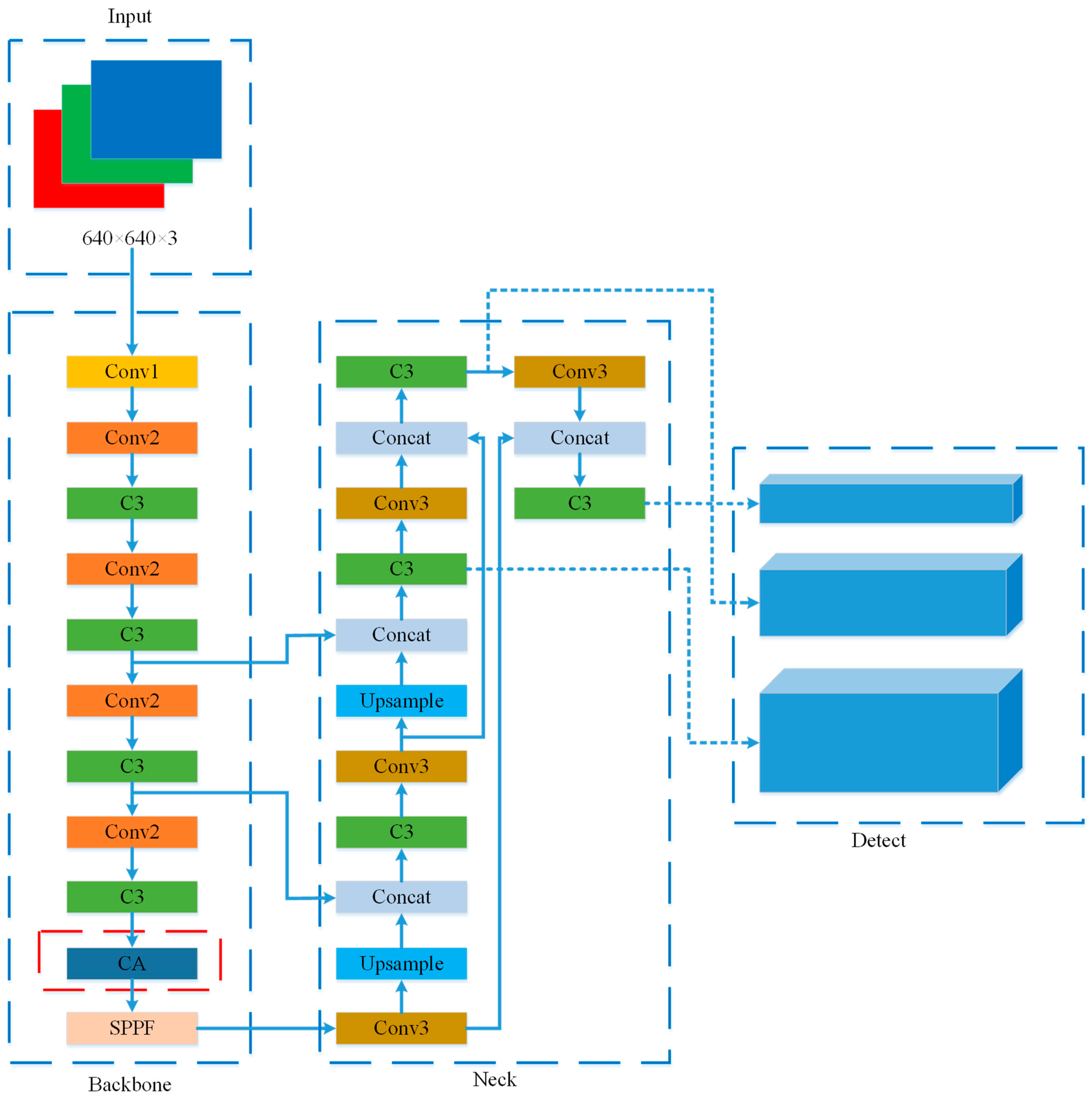
This paper uses the Yolov5 training dataset and adds the CA attention mechanism to the Yolov5 network. The improved network structure is shown in Figure 10, where the red wireframe indicates the position of the CA attention mechanism added. The improved Yolo network is divided into 25 layers, of which the ninth layer is the added CA attention module.
The Conv module in the Yolov5 network performs convolution, BN, and activation operations on the input feature maps; the C3 module is the main module for learning the residual features; the Upsample module has the primary purpose of enlarging the image and can increase the information of the image; the SPPF module fuses more features with different resolutions through pooling operations to get more information; the Concat module performs a fusion of the input feature maps; and detect module can predict the training results [32].

5. Fault-Line Selection Process

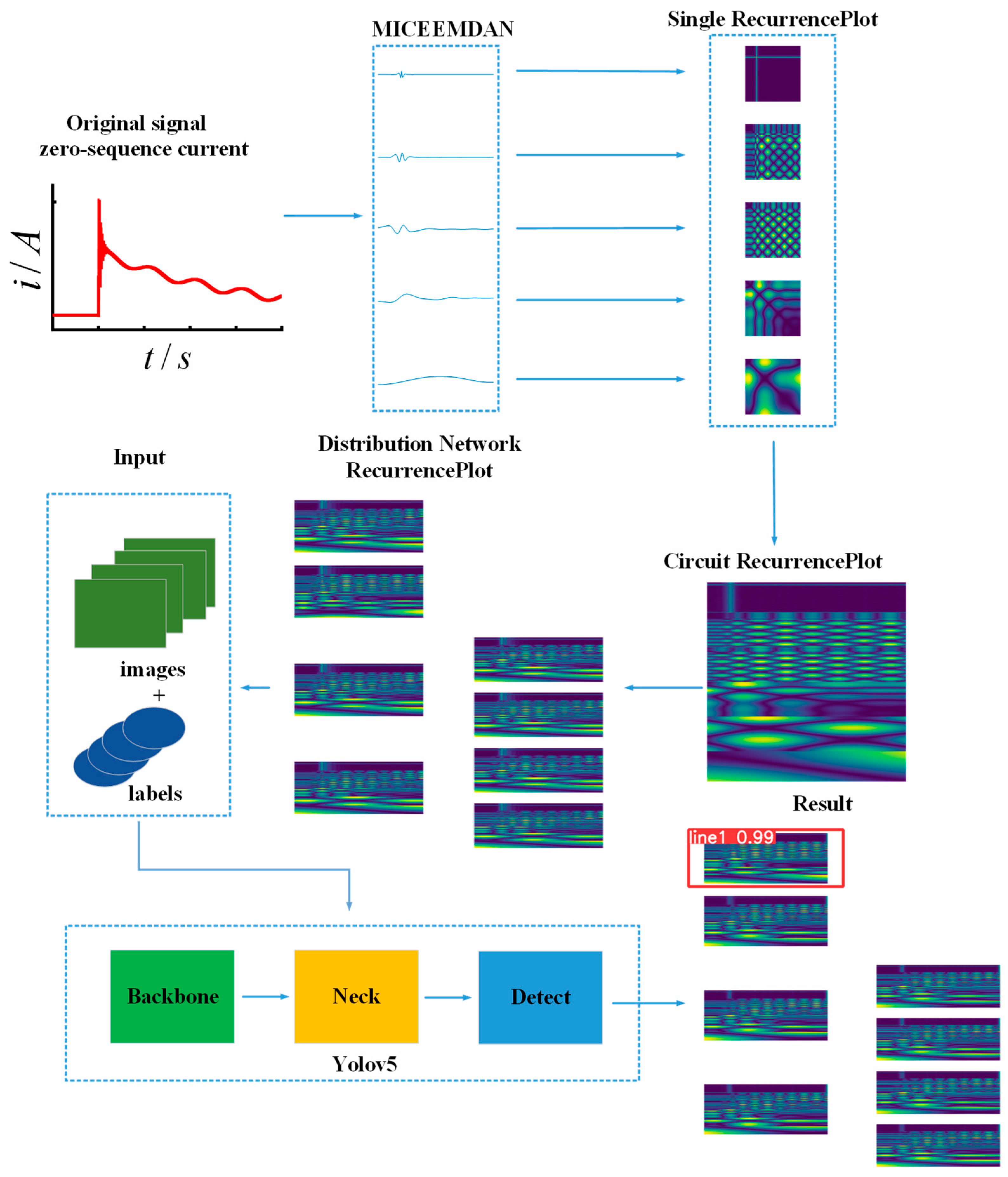
The fault routing process is shown in Figure 11, with the following steps.
Step 1: MICEEMDAN decomposition of zero-sequence currents is performed to obtain a series of eigenmodal functions.
Step 2: The decomposed eigenmodal functions are transformed into recurrence diagrams. All the obtained recurrence diagrams are stitched from top to bottom to obtain line recurrence diagrams, and all line recurrence diagrams are stitched to obtain distribution network recurrence diagrams.
Step 3: Annotate the obtained distribution network recurrence map to get the corresponding label file and use the image and the corresponding label as the input of the Yolov5 neural network.
Step 4: The Yolov5 neural network is used to train the model, and the model file is obtained.
Step 5: The model file generated by the training can be used to complete the single-phase ground fault routing in the distribution network.

6. Experimental Verification and Analysis

6.1. Simulation Environment

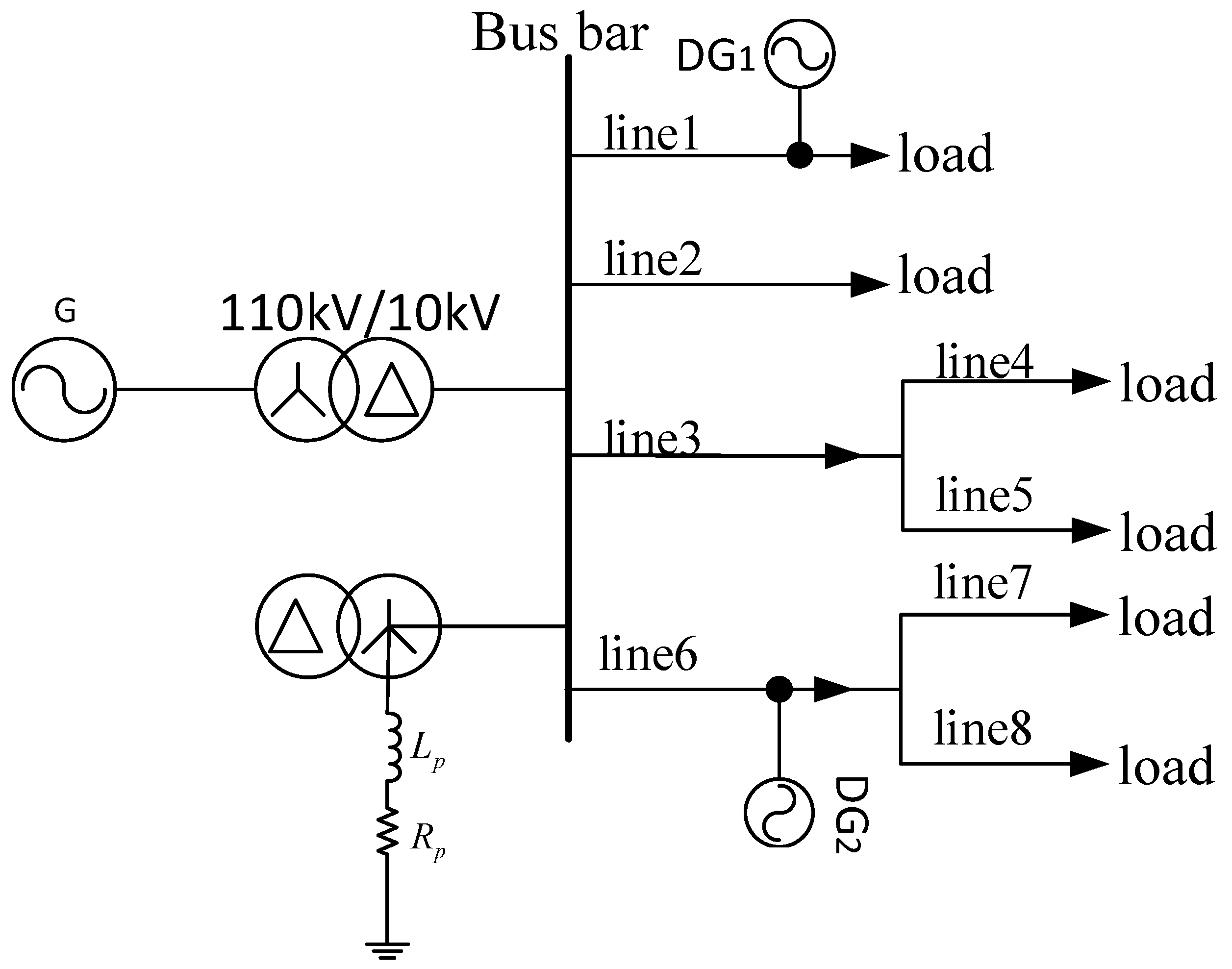
The topology of the 110 kV/10 kV distribution network system model, built based on MATLAB/Simulink, is shown in Figure 12. It contains four pure cable lines—Line 1, Line 3, Line 4, and Line 5, with lengths of 8 km, 4 km, 5 km, and 4 km—and four overhead lines—Line 2, Line 6, Line 7, and Line 8, with lengths of 10 km, 4 km, 5 km, and 6 km, respectively. The line parameters are shown in Table 2.
Using the overcompensation method, with an overcompensation degree of 10%, the equivalent inductance, LP = 1.907 H, and equivalent resistance, RL = 29.94 Ω, of the arc extinguishing coil were calculated.
In order to reduce the redundancy of the input neural network image, the recurrence maps of all lines were stitched together to construct the Recurrence Plot of the distribution network, as shown in Figure 13.

6.2. Feature Image Acquisition

In order to simulate the operation of the distribution network under actual working conditions, the fault line, fault phase, fault initial phase angle, fault ground resistance, and fault distance were set separately. The sampling frequency was 12.8 kHz; the system running time was 0.2 s; the fault phase was selected between phases A, B, and C; the fault initial phase angle was set to 0°, 30°, 60°, 90°, 120°, and 150°; the grounding resistance starts from 0 Ω and increases at an incremental rate of 100 Ω to 1500 Ω; and the fault distance starts from 2 km and increases at an incremental rate of 2 km to 2 km from the end of each line.
The original signals of one cycle before and two cycles after the fault in each section were sampled. The distribution network recurrence map and corresponding labels were generated according to the above fault selection process. In total, 4600 sets of images and corresponding labels were generated. The data were randomly selected according to the acquisition ratio of different fault types, 920 sets of which were used as the test set, and 3680 sets of data were used as the training set. In order to verify the robustness of the training results, 3 × 1000 recurrence maps of the distribution network were randomly generated by randomly changing the fault types and parameters as the validation set.

6.3. Line Selection Results in Verification and Analysis

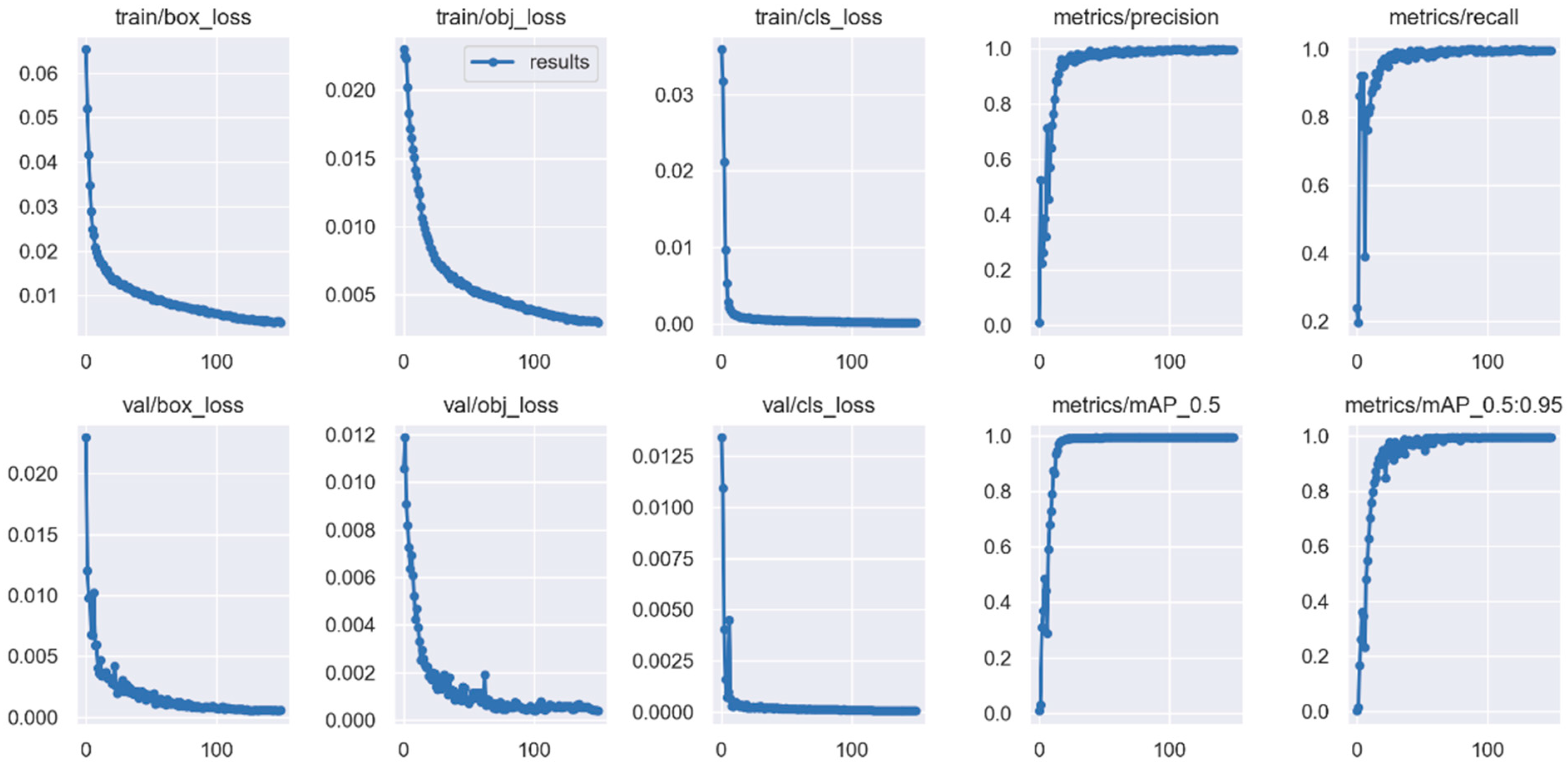
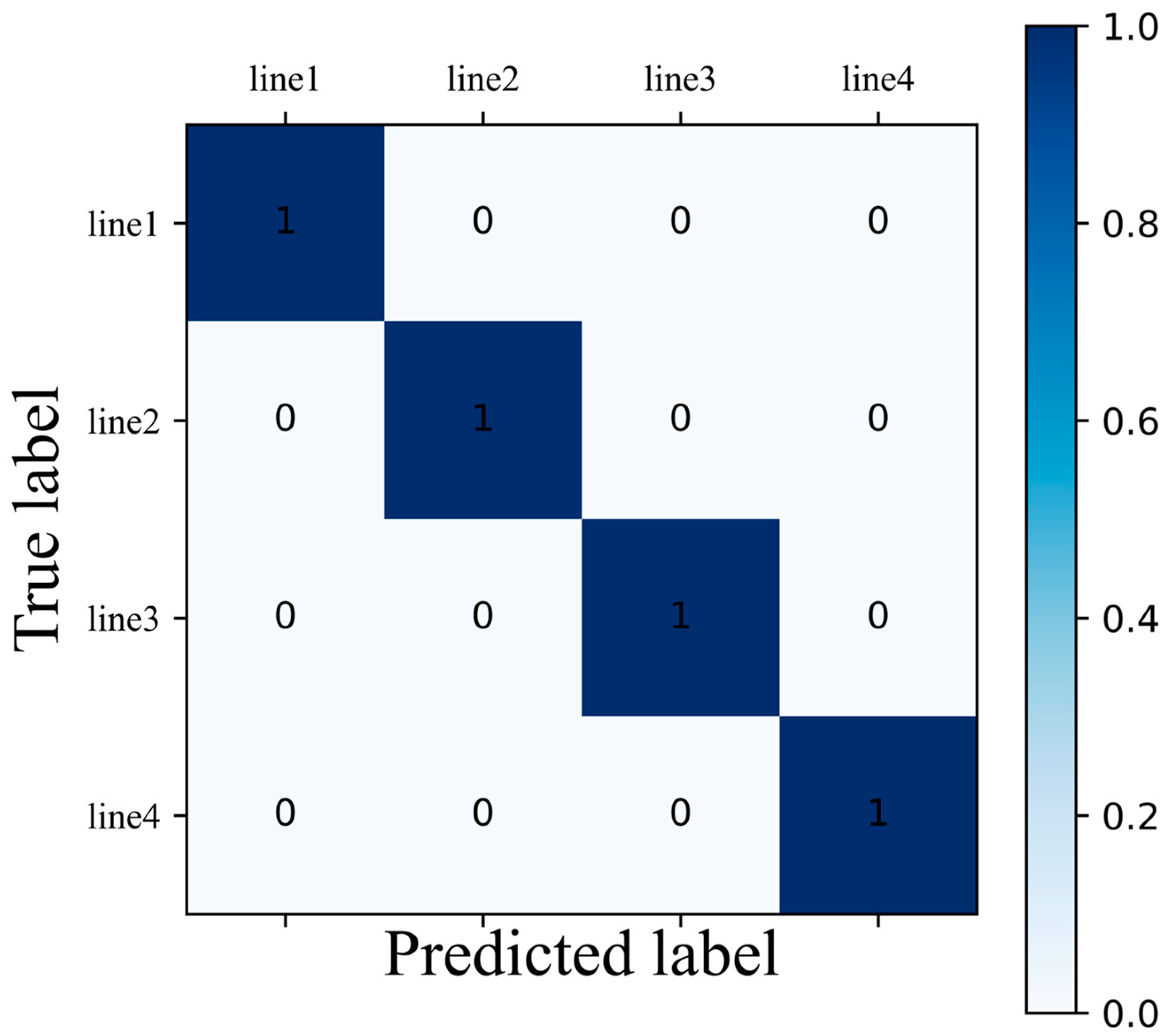
After training the model for 120 epochs, the model converged, and the loss function, accuracy, recall, and average precision mean were stabilized. The training number was set to 150 times, and the training results are shown in Figure 14. It can be seen from Figure 14 that with the increase in iterations, the box_loss, obj_loss, and cls_loss of both the training set and test set decreased and converged at 0. The precision, recall, and mAP increased, and the absolute accuracy of the model stabilized at 99.98%. The confusion matrix can show the training results more clearly. The confusion matrix obtained by analyzing the validation set is shown in Figure 15, where the diagonal cell values represent the percentage of correct selection results and the non-diagonal cell values represent the percentage of incorrect election results. It can be seen that the single-phase ground fault selection accuracy of the validation set reached 100%.
The optimal model obtained from the training was used to perform fault selection on the Recurrence Plot of the distribution network obtained from the simulation, and a rectangular box selected the fault section. In contrast, the fault information is indicated in the upper left corner. For a Line 1 ground fault, the fault distance of 2 km, 4 km, and 6 km, respectively, is shown in Figure 16; for a Line 2 ground fault, the initial phase angle of the fault is 0°, 60°, and 120°, respectively, and is shown in Figure 17. The Line 3 ground fault occurred at a grounding resistance of 10 Ω, 500 Ω, and 1500 Ω, and the selection results shown in Figure 18; a Line 4 ground fault occurred where the fault phase were A, B, and C phase selection, with the results shown in Figure 19.
As can be seen from the figure, with the change in fault conditions, some of the image features change, although there is no change visible to the naked eye; however, the training results show that the loss of the test set does not increase with the increase in training time, which is due to the Yolov5 neural network having the ability of autonomous mining of image features. For the small changes that the human eye cannot detect, the neural network can identify and extract these change features.
In order to verify that the model has a specific generalization ability, three rounds of validation were conducted using 1000 × 3 images of the distribution network Recurrence Plots generated by randomly changing the fault type and parameter way, and the validation results show that 3, 2, and 2 images of the three sets of images were misclassified, respectively, which indicates that the model has good generalization ability.
The experimental results show that the method is effective in different grounding resistances and fault initial phase angles, and the fault types have good performance and solid robustness.
The saved weight file of the Yolov5 model is only 14.2 Mb after 150 rounds of training, and the average recognition time is only 13.4 ms, which shows that the fault routing results are more satisfactory from various evaluation indexes.

6.4. Comparison Verification

6.4.1. Comparative Verification of Different Neural Networks

The color distribution of the neural network heat map reflects the attention weight of the neural network to the image. The darker the color, the greater the attention weight of the neural network, and the lighter the color, the smaller the attention weight of the neural network. Figure 20 shows the neural network heat map before and after adding the attention mechanism. It can be seen that when the attention mechanism is not added, the attention weight of the neural network is more randomly focused on each. After the attention mechanism is added, the attention points of the neural network are concentrated in the fault segment, and more attention weights are weighted on the practical part. Table 3 shows the training results before and after adding the attention mechanism. When the attention mechanism is not added, the convergence speed and accuracy of the network are decreased, and the results show that the neural network’s performance is improved after adding the attention mechanism.

6.4.2. Anti-Noise Comparison Verification

Under the actual working conditions, the raw electrical signal of the distribution network collected contains a large amount of noise. In order to verify that the proposed method in this paper has a specific noise immunity, the following methods are used, respectively.
Method 1: The acquired raw signal is directly transformed by a Recurrence Plot.
Method 2: EMD decomposition is performed on the original signal before Recurrence Plot transformation.
Method of this paper: The original signal is decomposed by MICEEMDAN and then transformed by a Recurrence Plot, which is the method proposed in this paper.
The Recurrence Plots obtained from the three methods are trained and tested with Yolov5 networks, and the results are shown in Table 4. It can be seen that performing MICEEMDAN decomposition first and then Recurrence Plot transformation can significantly improve the accuracy of the fault routing.
To further verify the noise immunity of the method in this paper, Gaussian white noise with different signal-to-noise ratios was added to the original signal, and the results are shown in Table 5 by comparing the method in this paper with the methods proposed in [14,19]. It can be seen that with the increase in the noise percentage, the proposed method in this paper still maintains a high accuracy of line selection, which indicates that the proposed method in this paper has good noise immunity.

6.4.3. High-Resistance Grounding Comparison Verification

When high-resistance grounding occurs, the fault signal features are not apparent, which affects the accuracy of the fault-sizing method. The method proposed in this paper converts one-dimensional data into two-dimensional images to fully extract the features. It fully exploits the features through neural networks, which has better sizing results in the case of high-resistance grounding, and the sizing accuracy can reach 99.93%. The method of this paper was compared with [14,19] by experiments, where the grounding resistance was set to 1000 and 1500, respectively. The experimental results are shown in Table 6. As seen in Table 6, the methods proposed in [14,19] both show misclassification in the case of high-resistance grounding, whereas the method used in this paper was still able to identify the faulty line correctly.

6.4.4. Distributed Generators Access

When the distribution network contains distributed generators, the following simulation experiments were conducted to verify the method’s feasibility in this paper.
In Figure 12, the distributed generator was connected to the end of Line 1 and Line 6, as shown in Figure 21. The following two models were tested separately.
(1) The original model is obtained by training when the distributed generator is not added.
(2) The new model is trained by re-collecting data using the proposed method.
The test results are shown in Table 7. When the distributed generators are connected to the distribution network, the accuracy of the proposed method for line selection without retraining the model is reduced. This is due to the change in fault characteristics after accessing the distributed power supply. The accuracy improves to 99.77% after retraining the model, indicating that the method in this paper is still applicable when the distributed generator is connected. The reason for the decrease in line selection accuracy compared with that before the access to distributed generators is that after the access to distributed generators, when the fault point is close to the access point of distributed generators, the attenuation of the non-periodic component of the zero sequence current becomes slower, which can cause misclassification.

6.4.5. Dynamic Mold Experiment

In order to verify the effectiveness of the proposed method in practical applications, in this paper we used a dynamic simulation fault diagnosis experimental platform laboratory for verification, as shown in Figure 22. The same simulation model as the dynamic simulation fault diagnosis experimental platform was built using MATLAB/Simulink, as shown in Figure 23, including three lines: Line 1 is an overhead line; Line 2 is a cable line; and Line 3 is a mixed overhead and cable line.
A simulation model was used to collect the data, train the model, and test the line selection accuracy of the model using the data collected in the dynamic simulation fault diagnosis experimental platform. The test results are shown in Table 8. It can be seen from Table 8 that the method proposed in this paper can accurately select fault lines under actual working conditions, which confirms the practicality of the method proposed in this paper in practical scenarios.

7. Conclusions

This paper proposes a new distribution network fault routing method using the MICEEMDAN–Recurrence Plot–Yolov5 network, and the research results are as follows.
(1) MWPE can solve the problem of MPE’s lack of sensitivity to abrupt signals. A new signal noise reduction and decomposition algorithm, MICEEMDAN, is proposed based on MWPE and ICEEMDAN. The simulation results show that MICEEMDAN suppresses modal confusion, reduces the appearance of pseudo-modal components, and has better decomposition effects than the existing algorithms.
(2) The Recurrence Plot algorithm converts one-dimensional time series into two-dimensional images. All fault features are concentrated on one image by stitching twice to fully exploit the minute features of one-dimensional signals.
(3) The addition to the CA attention mechanism, the Yolov5 network makes the neural network pay more attention to the feature extraction of the fault segment part, which accelerates the convergence speed of the model and improves the accuracy of the fault routing.
The experimental results show that compared with the traditional fault routing method, the method is not affected by the fault type, fault moment, and transition resistance; has strong noise immunity and stability; and can accurately determine the fault line, with the accuracy in fault type identification able to reach 99.98%. This study provides a new idea for distribution network fault-line selection research.

Author Contributions

Conceptualization, S.H., Y.X. and W.G.; methodology, S.H.; software, Y.X.; validation, S.H., Y.X. and W.G.; formal analysis, S.H.; investigation, Y.X.; resources, S.H., Y.X. and W.G.; data curation, Y.X.; writing—original draft preparation, S.H., Y.X. and W.G.; writing—review and editing, Y.X.; visualization, S.H., Y.X. and W.G.; supervision, S.H.; project administration, S.H. All authors have read and agreed to the published version of the manuscript.

Funding

This work was supported by the National Key R&D Program of China (Grant no. 2018YFF01011900).

Data Availability Statement

Not applicable.

Conflicts of Interest

The authors declare no conflict of interest.

Nomenclature

ICEEMDANImproved Complete Ensemble Empirical Mode Decomposition Adaptive Noise
MICEEMDANmodifying the Improved Complete Ensemble Empirical Mode Decomposition Adaptive Noise
PEpermutation entropy
MPEmulti-scale permutation entropy
MWPEmulti-scale weighted permutation entropy
IMFsintrinsic mode functions
VMDvariational modal decomposition
CNNconvolutional neural network
CAcoordinate attention

References

  1. Zhang, X.; Tai, N.; Wu, P.; Zheng, X.; Huang, W. A fault line selection method for DC distribution network using multiple observers. Energies 2019, 12, 1245. [Google Scholar] [CrossRef] [Green Version]
  2. Su, X.; Wei, H. A fault-line selection method for small-current grounded system based on deep transfer learning. Energies 2022, 15, 3467. [Google Scholar] [CrossRef]
  3. Cheng, H.-J.; Meng, H.; Jiang, P.-J. Research on fault line selection in small-current neutral grounding power system. In Proceedings of the 2013 IEEE International Conference on Vehicular Electronics and Safety, Dongguan, China, 28–30 July 2013; pp. 206–209. [Google Scholar] [CrossRef]
  4. Liao, K.; Du, Y.; Dong, K.; Fan, H.; Zhao, X. Identification of Fault Line Selection and Section for Single-Phase Ground Fault in Small Current Grounding System. In Proceedings of the 2020 5th International Conference on Power and Renewable Energy (ICPRE), Shanghai, China, 12–14 September 2020; pp. 267–271. [Google Scholar] [CrossRef]
  5. Shuping, G.; Bicong, D.; Guobing, S.; Mingxing, S. Fault line selection method of DC distribution network based on transient current fault component. In Proceedings of the 2020 7th International Forum on Electrical Engineering and Automation (IFEEA), Hefei, China, 25–27 September 2020; pp. 433–437. [Google Scholar] [CrossRef]
  6. Liang, S.; Zhang, Z. Single-Phase ground fault traveling wave line selection method and line selection device field test. In Proceedings of the 2018 2nd IEEE Conference on Energy Internet and Energy System Integration (EI2), Beijing, China, 20–22 October 2018; pp. 1–4. [Google Scholar] [CrossRef]
  7. Zhengyi, L.; Changhong, D.; Huamei, Y.; Hu, F. A LSTM line selection method of single-phase ground fault based on big-data platform. In Proceedings of the 2021 3rd Asia Energy and Electrical Engineering Symposium (AEEES), Chengdu, China, 26–29 March 2021; pp. 776–780. [Google Scholar] [CrossRef]
  8. Liu, B.; Ma, H.; Xu, H.; Ju, P. Single-phase-to-ground fault detection with distributed parameters analysis in non-direct grounded systems. CSEE J. Power Energy Syst. 2019, 5, 139–147. [Google Scholar] [CrossRef]
  9. Chang, Z.; Song, G.; Huang, W.; Guo, S.; Zhang, W. Phase voltage and current fault components based fault segment location method under single-phase earth fault in distribution network. Power Syst. Technol. 2020, 41, 2363–2369. [Google Scholar] [CrossRef]
  10. Yang, X.; Liu, W. A new line selection method based on intrinsic mode energy of phase current change. J. Electr. Power Sci. Technol. 2018, 33, 149–154. [Google Scholar] [CrossRef]
  11. Yang, F.; Liu, X.X.; Shen, Y. Low-resistance grounding system high-resistance ground fault protection based on zero sequence current projection coefficient. Power Syst. Technol. 2020, 44, 1128–1133. [Google Scholar]
  12. Gao, L.; Wu, S.; Wang, M.; Wang, Z.; Yang, Y. Single-line-to-ground fault line selection method in distribution network based on multi-scale wavelet decomposition of transient signals. In Proceedings of the 2022 7th International Conference on Intelligent Computing and Signal Processing (ICSP), Xi’an, China, 15–17 April 2022; pp. 2052–2057. [Google Scholar] [CrossRef]
  13. Qingshan, Q.; Xiuying, X.; Chongyi, T.; Ruiqi, W. Single-phase ground fault location of distribution network with DG based on CEEMD. In Proceedings of the 2020 Asia Energy and Electrical Engineering Symposium (AEEES), Chengdu, China, 29–31 May 2020; pp. 587–591. [Google Scholar] [CrossRef]
  14. Hou, S.; Guo, W. Optimal denoising and feature extraction methods using modified CEEMD combined with duffing system and their applications in fault line selection of non-solid-earthed network. Symmetry 2020, 12, 536. [Google Scholar] [CrossRef] [Green Version]
  15. Ray, P.; Mishra, D.P.; Dey, K.; Mishra, P. Fault detection and classification of a transmission line using discrete wavelet transform & artificial neural network. In Proceedings of the 2017 International Conference on Information Technology (ICIT), Bhubaneswar, India, 21–23 December 2017; pp. 178–183. [Google Scholar] [CrossRef]
  16. Luo, G.; Tan, Y.; Li, M.; Cheng, M.; Liu, Y.; He, J. Stacked auto-encoder-based fault location in distribution network. IEEE Access 2020, 8, 28043–28053. [Google Scholar] [CrossRef]
  17. Jayamaha, D.K.J.S.; Lidula, N.W.A.; Rajapakse, A.D. Wavelet-multi resolution analysis based ANN architecture for fault detection and localization in DC microgrids. IEEE Access 2019, 7, 145371–145384. [Google Scholar] [CrossRef]
  18. Tabatabaei, A.; Mosavi, M.R.; Farajiparvar, P. A traveling-wave fault location technique for three-terminal lines based on wavelet analysis and Recurrent Neural Network using GPS timing. In Proceedings of the 2013 Smart Grid Conference (SGC), Tehran, Iran, 17–18 December 2013; pp. 268–272. [Google Scholar] [CrossRef]
  19. Liang, J. Research on rapid diagnosis method of single-phase grounding fault in distribution network based on deep learning. In Proceedings of the 2019 Chinese Automation Congress (CAC), Hangzhou, China, 22–24 November 2019; pp. 20–24. [Google Scholar] [CrossRef]
  20. Cheng, X.-R.; Cui, B.-J.; Hou, S.-Z. Fault line selection of distribution network based on modified CEEMDAN and GoogLeNet neural network. IEEE Sens. J. 2022, 22, 13346–13364. [Google Scholar] [CrossRef]
  21. Hou, S.; Guo, W. Fault identification method for distribution network based on parameter optimized variational mode decomposition and convolutional neural network. IET Gener. Transm. Distrib. 2022, 16, 737–749. [Google Scholar] [CrossRef]
  22. Zhang, H.; He, S.-S. Analysis and comparison of permutation entropy, approximate entropy and sample entropy. In Proceedings of the 2018 International Symposium on Computer, Consumer and Control (IS3C), Taichung, Taiwan, 6–8 December 2018; pp. 209–212. [Google Scholar] [CrossRef]
  23. Peng, Z.; Zhang, X.; Cao, J.; Liu, B. Recognition of biological tissue denaturation based on improved multiscale permutation entropy and GK fuzzy clustering. Information 2022, 13, 140. [Google Scholar] [CrossRef]
  24. Zheng, J.; Liu, T.; Meng, R.; Liu, Q. Generalized composite multiscale permutation entropy and PCA based fault diagnosis of rolling bearings. J. Vib. Shock 2018, 37, 61–66. [Google Scholar]
  25. Zheng, J.D.; Cheng, J.H.; Yang, Y. Modified EEMD algorithm and its applications. J. Vib. Shock 2013, 32, 21–26. [Google Scholar]
  26. Zhao, Y.; Adjallah, K.H.; Sava, A. Influence study of the intermittent wave amplitude vs. the sampling frequency ratio on ICEEMDAN mode mixing alleviation performance. In Proceedings of the 2018 IEEE 23rd International Conference on Digital Signal Processing (DSP), Shanghai, China, 19–21 November 2018; pp. 1–5. [Google Scholar] [CrossRef]
  27. Das, A.B.; Bhuiyan, M.I.H. Discrimination of focal and non-focal EEG signals using entropy-based features in EEMD and CEEMDAN domains. In Proceedings of the 2016 9th International Conference on Electrical and Computer Engineering (ICECE), Dhaka, Bangladesh, 20–22 December 2016; pp. 435–438. [Google Scholar] [CrossRef]
  28. Wang, X.; Gao, J.; Song, G.; Cheng, Q.; Wei, X.; Wei, Y. Faulty line selection method for distribution network based on variable scale bistable system. J. Sens. 2016, 2016, 1–17. [Google Scholar] [CrossRef] [Green Version]
  29. Wang, Z.; Qiao, P.; Shi, B. Nonpenetrating damage identification using hybrid lamb wave modes from Hilbert-Huang spectrum in thin-walled structures. Shock Vib. 2017, 2017, 1–11. [Google Scholar] [CrossRef] [Green Version]
  30. Moraes, A.L.; Fernandes, R.A.S. Recurrence Plots: A novel feature engineering technique to analyze power quality disturbances. In Proceedings of the 2020 IEEE Power & Energy Society General Meeting (PESGM), Montreal, QC, Canada, 2–6 August 2020; pp. 1–5. [Google Scholar] [CrossRef]
  31. Hou, Q.; Zhou, D.; Feng, J. Coordinate attention for efficient mobile network design. In Proceedings of the 2021 IEEE/CVF Conference on Computer Vision and Pattern Recognition (CVPR), Nashville, TN, USA, 20–25 June 2021; pp. 13708–13717. [Google Scholar] [CrossRef]
  32. Li, Q.; Zhao, F.; Xu, Z.; Wang, J.; Liu, K.; Qin, L. Insulator and damage detection and location based on Yolov5. In Proceedings of the 2022 International Conference on Power Energy Systems and Applications (ICoPESA), Singapore, 25–27 February 2022; pp. 17–24. [Google Scholar] [CrossRef]
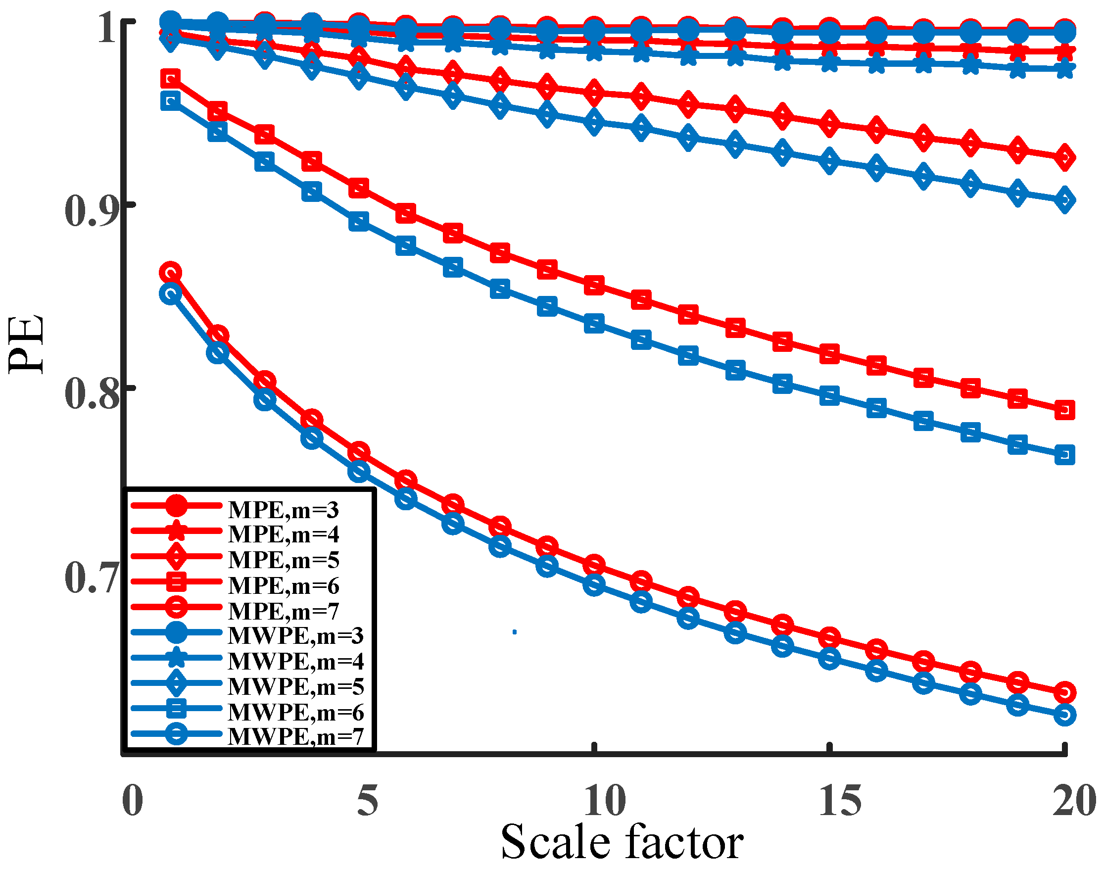
Figure 1. Multi-scale permutation entropy and multi-scale weighted permutation entropy of white noise with different scale factors and embedding dimensions.
Processes 10 02127 g001
Figure 2. Adding pulses to white noise.
Processes 10 02127 g002
Figure 3. Permutation entropy results.
Processes 10 02127 g003
Figure 4. The original simulation signal.
Processes 10 02127 g004
Figure 5. The decomposition results: (a) ICEEMDAN; (b) MICEEMDAN.
Processes 10 02127 g005
Figure 6. Correlation coefficients of the original simulation signal decomposition results of the two methods.
Processes 10 02127 g006
Figure 7. Hilbert–Huang spectrum: (a) ICEEMDAN; (b) MICEEMDAN.
Processes 10 02127 g007
Figure 8. Generated Recurrence Plots: (a) grounding resistance 10 Ω; (b) grounding resistance 500 Ω; (c) grounding resistance 1500 Ω; (d) Phase A grounded; (e) Phase B grounded; (f) Phase C grounded; (g) initial phase angle 0°; (h) initial phase angle 60°; (i) initial phase angle 120°; (j) fault distance 2 km; (k) fault distance 4 km; (l) fault distance 6 km.
Processes 10 02127 g008
Figure 9. CA module structure.
Processes 10 02127 g009
Figure 10. Improved Yolov5 network structure.
Processes 10 02127 g010
Figure 11. Fault-line selection process.
Processes 10 02127 g011
Figure 12. Distribution network.
Processes 10 02127 g012
Figure 13. Distribution network Recurrence Plot.
Processes 10 02127 g013
Figure 14. Yolov5 training results.
Processes 10 02127 g014
Figure 15. Identification of the confusion matrix.
Processes 10 02127 g015
Figure 16. Grounding fault that occurred in Line 1: fault distance of (a) 2 km; (b) 4 km; (c) 6 km.
Processes 10 02127 g016
Figure 17. Grounding fault that occurred in Line 2: fault initial phase (a) 0°; (b) 60°; (c) 120°.
Processes 10 02127 g017
Figure 18. Grounding fault that occurred in Line 3: ground resistance of (a) 10 Ω; (b) 500 Ω; (c) 1500 Ω.
Processes 10 02127 g018
Figure 19. Grounding fault that occurred in Line 4: fault phase of (a) A; (b) B; (c) C.
Processes 10 02127 g019
Figure 20. Neural network heat map before and after adding the attention mechanism: (a) no attention mechanism added; (b) add attention mechanism.
Processes 10 02127 g020
Figure 21. Distribution network with distributed generators.
Processes 10 02127 g021
Figure 22. Dynamic simulation fault diagnosis experimental platform.
Processes 10 02127 g022
Figure 23. Experimental model of the dynamic fault simulation system.
Processes 10 02127 g023
Table 1. Multi-scale permutation entropy and multi-scale weighted permutation entropy of each signal.
SignalMulti-Scale Permutation
Entropy
Multi-Scale Weighted Permutation Entropy
White noise0.90870.8918
Gaussian white noise0.91120.8896
High-frequency sinusoidal signal0.43100.4162
Fundamental frequency sinusoidal signal0.11760.1053
AM signal0.51520.4541
FM signal0.37530.3809
AM/FM signal0.53710.4981
Intermittent signal0.58880.8402
Table 2. Simulation model line parameters.
Circuit TypeResistance/
(Ω·km−1)
Inductance/
(mH·km−1)
Grounding Capacitance/
(μF·km−1)
Positive PhaseZero PhasePositive PhaseZero PhasePositive PhaseZero Phase
Overhead line0.1780.251.215.540.0150.012
Cable line0.272.70.2551.020.3390.28
Table 3. Comparison of results before and after adding the CA attention mechanism.
MethodsTraining RoundsAccuracy/%
Yolov530099.31
Yolov5 + CA15099.98
Table 4. Comparison of the noise immunity of the different methods.
LineNumber of SamplesAccuracy/%
Method 1Method 2Method of This Paper
Line 150092.9196.8999.98
Line 260093.1895.9499.99
Line 380090.7293.8799.97
Line 480091.8693.8999.98
Table 5. Comparison of line selection accuracy under different signal-to-noise ratios.
Signal-to-Noise Ratio/dBLineNumber of SamplesAccuracy/%
Ref. [14]Ref. [19]This Paper
35Line 150096.9198.3399.98
Line 260096.8398.3099.99
Line 380094.2197.5199.97
Line 480094.7397.5499.98
30Line 150094.7195.3199.97
Line 260094.6795.1299.98
Line 380093.1192.7899.97
Line 480093.0293.0299.98
25Line 150090.6791.2599.96
Line 260088.3291.1299.98
Line 380087.9190.4299.95
Line 480087.0590.6199.95
20Line 150084.8488.1599.94
Line 260084.3288.3299.95
Line 380082.5986.8999.93
Line 480082.5185.9199.94
Table 6. Comparison of the experimental results of high-resistance grounding.
Grounding Resistance/ΩLine Line Selection Results
Ref. [14]Ref. [19]This Paper
1000Line 1Line 1Line 1Line 1
Line 2Line 2Line 2Line 2
Line 3Line 2Line 3Line 3
Line 4Line 4Line 4Line 4
1500Line 1Line 1Line 1Line 1
Line 2Line 2Line 2Line 2
Line 3Line 2Line 3Line 3
Line 4Line 3Line 3Line 4
Table 7. Line selection results after distributed generators access.
LineNumber of SamplesAccuracy/%
Original ModelNew Model
Line 150097.9399.75
Line 260098.1999.87
Line 380098.1299.79
Line 480097.8699.69
Table 8. Line selection results under the conditions of the dynamic simulation fault diagnosis experimental platform.
Fault TypeFault Line Fault PointTransition ResistanceFault Close AngleFault Line
Selection Result
AGLine 1F10 ΩLine 1
BGLine 1F2500 Ω30°Line 1
CGLine 1F31000 Ω60°Line 1
AGLine 2F1400 Ω60°Line 2
BGLine 2F2800 Ω120°Line 2
CGLine 2F3200 Ω30°Line 2
BGLine 2F4500 Ω150°Line 2
AGLine 3F10 ΩLine 3
CGLine 3F2400 Ω60°Line 3
Publisher’s Note: MDPI stays neutral with regard to jurisdictional claims in published maps and institutional affiliations.