Accurate Effective Diffusivities in Multicomponent Systems

Abstract

Mass transfer is an omnipresent phenomenon in the chemical and related industries for which effective diffusivities ($D_{i,\mathrm{eff}}$) constitute a useful and simple mathematical tool, especially when dealing with multicomponent mixtures. Although several models have been published for $D_{i,\mathrm{eff}}$ they generally involve simplifying assumptions that severely restrict their use. The current work presents the derivation of accurate analytical equations for $D_{i,\mathrm{eff}}$, which take into account the nonideal behavior of multicomponent mixtures. Additionally, it is demonstrated that for an ideal mixture the new model reduces to the well-known equations of Bird et al., which are the exact analytical solution for ideal systems. The procedure for $D_{i,\mathrm{eff}}$ estimation is described in detail and exemplified with two chemical reactions: the liquid phase ethyl acetate synthesis and the high pressure gas phase methanol synthesis. Relative to the Bird et al. ideal equations the effective diffusivities calculated with the new model show differences up to 38% for ethyl acetate synthesis when using UNIFAC model to evaluate activity coefficients. For methanol synthesis, deviations from −23% to 22% are found using PC-SAFT equation of state (EoS) and from −49% to 24% when applying the Peng–Robinson EoS to estimate fugacity coefficients. Comparisons are also performed with the models by Wilke, Burghardt and Krupiczka, Kubota et al., and Kato et al. The worst results are achieved by the Wilke and Kubota et al. equations for the liquid phase and gas phase reactions, respectively. Furthermore, it is shown that substantial errors in effective diffusivity calculations may occur when deviations from the ideal behavior are unaccounted for. This can be avoided by adopting the new rigorous approach here presented.

1. Introduction

Several areas within the chemical industry, ranging from chemical reactions (catalysis) to separation processes (e.g., adsorption, membranes, extractions), involve multicomponent mixtures. The mathematical description of diffusion mass transfer in such situations becomes increasingly complex when compared with the simplicity of Fick’s first law for binary mixtures, especially when deviations from the ideal behavior (ideal gas or ideal solution) need to be accounted for. Significant drawbacks in process design involving nonideal mixtures may appear if failing to do so. In the particular case of heterogeneous reactors, the precise description of diffusion will impact the reactor mass balance equations (e.g., axial and radial dispersion models) and even the observable reaction rate (e.g., internal and external diffusion limitations) [1].

One approach to describe the molar diffusion flux in multicomponent mixtures is Fick’s generalized equation, which in matrix representation is given by:

$$\left(\overline{J}\right)=-C_T\left[D\right](\nabla x)$$

(1)

where $\left(\overline{J}\right)$ is the molar diffusion flux vector, $C_T$ is the total concentration of the mixture, and $(\nabla x)$ is the mole fraction gradient vector. For a system of n components, $\left[D\right]$ is an $(n-1)\times (n-1)$ matrix in which the $D_{ij}$ pair diffusion coefficients are not symmetric and do not hold the same physical meaning as the binary diffusion coefficients [2].

An alternative approach to describe multicomponent mass transfer is by Maxwell–Stefan equations, which can be made explicit in terms of the molar diffusion flux. In matrix notation, for a mixture of n components, $\left(\overline{J}\right)$ is described by [2]:

$$\begin{array}{c}\left(\overline{J}\right)=-C_T{\left[B\right]}^{-1}[\Gamma ](\nabla x)\end{array}$$

(2a)

$$\begin{array}{c}{B}_{ii}=\frac{x_i}{{Ð}_{in}}+\sum _{\begin{array}{c}j=1\\ j\ne i\end{array}}^n\frac{x_j}{{Ð}_{ij}}\end{array}$$

(2b)

$$\begin{array}{c}{B}_{ij}=-x_i\left(\frac{1}{{Ð}_{ij}}-\frac{1}{{Ð}_{in}}\right)\end{array}$$

(2c)

$$\begin{array}{c}{\Gamma }_{ij}={\delta }_{ij}+x_i\frac{\partial ln{\gamma }_i}{\partial x_j}{|}_{P,T,x_k[k=1,2,\dots ,n-1,k\ne j]}\end{array}$$

(2d)

$$\begin{array}{c}{\delta }_{ij}=\frac{\partial x_i}{\partial x_j}=\left\{\begin{array}{c}{\delta }_{ij}=0,i\ne j\hfill \\ {\delta }_{ij}=1,i=j\hfill \end{array}\right.\end{array}$$

(2e)

where $\left[B\right]$ is an $(n-1)$ square matrix with main diagonal elements $B_{ii}$ and off-diagonal elements $B_{ij}$, $[\Gamma ]$ is an $(n-1)$ square matrix with elements ${\Gamma }_{ij}$, ${Ð}_{ij}$ represents the Maxwell–Stefan diffusivity of $ij$ pair, ${\gamma }_i$ is the activity coefficient of component i, and ${\delta }_{ij}$ is the Kronecker function. In physical terms ${Ð}_{ij}$ is equivalent to the inverse of a drag or friction coefficient [2]. For a mixture of gases ${\gamma }_i$ is replaced by the fugacity coefficient, ${\widehat{\varphi }}_i$.

Equation (2a) is more rigorous than Equation (1), as deviations from the ideal behavior (evaluated with an equation of state or activity coefficient model) can be incorporated into ${\Gamma }_{ij}$. However, due to the mathematical complexity of both approaches [2], a few simplified methods have been developed over the years, such as the effective diffusivity concept, which can be particularly advantageous for computing fluxes in material balances. The effective diffusivity models express the molar diffusion flux of a component i, ${\overline{J}}_i$, uniquely as function of its composition gradient, $\nabla x_i$ [2]:

$${\overline{J}}_i=-C_T{D}_{i,\mathrm{eff}}\nabla x_i$$

(3)

where $D_{i,\mathrm{eff}}$ is the effective diffusivity of species i. In matrix notation, it is given by:

$$\left(\overline{J}\right)=-C_T\left[D_{\mathrm{eff}}\right](\nabla x)$$

(4)

where $\left[D_{\mathrm{eff}}\right]$ is an $(n-1)\times (n-1)$ diagonal matrix containing the effective diffusivities. Several equations to compute effective diffusivities have been published in the literature. Wilke [3] developed a specific model for the unimolecular diffusion of a species i through a film of stagnant gases:

$$D_{i,\mathrm{eff}}^W=\frac{1-x_i}{{\sum }_{\begin{array}{c}j=1\\ j\ne i\end{array}}^n\frac{x_j}{{Ð}_{ij}}}$$

(5)

Bird et al. [4] presented the exact analytical solution for the effective diffusivity in an ideal mixture, which is given by:

$$D_{i,\mathrm{eff}}^{Ideal}=\frac{{\overline{N}}_i-{\overline{N}}_T{x}_i}{{\overline{N}}_i{\sum }_{\begin{array}{c}j=1\\ j\ne i\end{array}}^n\frac{x_j}{{Ð}_{ij}}-x_i{\sum }_{\begin{array}{c}j=1\\ j\ne i\end{array}}^n\frac{{\overline{N}}_j}{{Ð}_{ij}}}$$

(6)

where ${\overline{N}}_i$ is the molar flux of i, and ${\overline{N}}_T$ is the total molar flux. The molar flux is related with the molar diffusion flux via the fundamental equation ${\overline{N}}_i={\overline{J}}_i+x_i{\overline{N}}_T$. Kubota et al. [5] reported an approximate model based on Equation (6), which was used to calculate catalyst effectiveness in a three component gas mixture and is represented by:

$$\frac{1}{D_{i,\mathrm{eff}}^K}=\sum _{\begin{array}{c}j=1\\ j\ne i\end{array}}^n\frac{x_j}{{Ð}_{ij}}\left(1-\frac{x_i{\overline{N}}_j}{x_j{\overline{N}}_i}\right)$$

(7)

Burghardt and Krupiczka developed a model for ideal mixtures in which the off-diagonal elements of matrix $\left[B\right]$ were neglected [2]:

$$\frac{1}{D_{i,\mathrm{eff}}^{BK}}=B_{ii}=\frac{x_i}{{Ð}_{in}}+\sum _{\begin{array}{c}j=1\\ j\ne i\end{array}}^n\frac{x_j}{{Ð}_{ij}}$$

(8)

Kato et al. [6] elaborated a model similar to Equation (8) by neglecting the off-diagonal elements of matrix $\left[D\right]$ [2], which is expressed by:

$$D_{i,\mathrm{eff}}^{Kato}=D_{ii}$$

(9)

As can be seen, each equation has its intrinsic limitations due to the simplifying assumptions made during their respective derivations, such as assuming ideal gas behavior and/or unimolecular diffusion (stagnant film). This may introduce large errors and poor predictive capabilities when these equations are used outside the scope for which they were developed. The goal of this work is to present a new effective diffusivity model, which is more rigorous in its approach, taking into consideration the nonideal behavior of a mixture in the form of activity coefficients (for liquids) or fugacity coefficients (for gases). For comparison purposes, the performance of the new model and the aforementioned approaches are analyzed using two case studies: (1) a liquid phase reaction (ethyl acetate synthesis) and (2) a gas phase reaction under high pressure (methanol synthesis).

2. New Effective Diffusivity Model

In this section the rigorous effective diffusivity model is derived and the basic steps required for its application are delineated. It is also shown that, in the case of ideal mixtures, the new model reduces to the equation developed by Bird et al. [4]. More derivation details are described in the supporting information.

2.1. Derivation of Model Equations

For an arbitrary composition gradient $(\nabla x)$ the molar diffusion flux $\left(\overline{J}\right)$ calculated with Equation (2a) should yield the same result as the one obtained using effective diffusivities, Equation (4). Thus, the following relation between matrices ${\left[D_{\mathrm{eff}}\right]}^{-1}$ and ${\left[D\right]}^{-1}$ must be satisfied:

$${\left[D_{\mathrm{eff}}\right]}^{-1}\left(\overline{J}\right)={\left[D\right]}^{-1}\left(\overline{J}\right),\mathrm{where}\left[D\right]={\left[B\right]}^{-1}[\Gamma ]$$

(10)

Since $\left[D_{\mathrm{eff}}\right]$ is a diagonal matrix the elements of its inverse are simply given by the inverse of the original matrix elements. The ith row of Equation (10) is given by:

$$\frac{1}{D_{i,\mathrm{eff}}}=\sum _{j=1}^{n-1}{D}_{ij}^{inv}\frac{{\overline{J}}_j}{{\overline{J}}_i}$$

(11)

where $D_{ij}^{inv}$ represents the $ij$ element of matrix ${\left[D\right]}^{-1}$. Hence, Equation (11) allows one to calculate the effective diffusivities for the first $n-1$ components. It is also possible to derive an equation for the effective diffusivity of the last component n, $D_{n,\mathrm{eff}}$. First, recalling that $x_n=1-{\sum }_{j=1}^{n-1}{x}_j$, the molar diffusion flux of component n gives:

$${\overline{J}}_n=-C_T{D}_{n,\mathrm{eff}}\nabla x_n=C_T{D}_{n,\mathrm{eff}}\sum _{j=1}^{n-1}\nabla x_j$$

(12)

Moreover, since $\nabla x_j=-{\overline{J}}_j/\left(D_{j,\mathrm{eff}}{C}_T\right)$ the molar diffusion flux of species n becomes:

$${\overline{J}}_n=-D_{n,\mathrm{eff}}\sum _{j=1}^{n-1}\frac{{\overline{J}}_j}{D_{j,\mathrm{eff}}}$$

(13)

which can be rearrenged as:

$$\frac{1}{D_{n,\mathrm{eff}}}=-\sum _{j=1}^{n-1}\frac{1}{D_{j,\mathrm{eff}}}\frac{{\overline{J}}_j}{{\overline{J}}_n}$$

(14)

This equation can be used to calculate $D_{n,\mathrm{eff}}$ after computing all $D_{j,\mathrm{eff}}$, with $j=1,\dots ,(n-1)$ via Equation (11).

2.2. Calculation Procedure

The following steps are necessary to calculate the effective diffusivities using the new model:

• Using tabulated experimental data or empirical correlations, collect the binary diffusion coefficients at infinite dilution of all $ij$ pairs of components, $D_{ij}^{°}$. These are equal to the infinite dilution binary Maxwell–Stefan (MS) diffusion coefficients, ${Ð}_{ij}^{°}=D_{ij}^{°}$.
• Compute the MS diffusion coefficients, ${Ð}_{ij}$, for the specific mixture composition using the following mixing rule:

  $${Ð}_{ij}={({Ð}_{ij}^{°})}^{(1-x_i+x_j)/2}·{({Ð}_{ji}^{°})}^{(1-x_j+x_i)/2}$$

  (15)
  In the special case of binary mixtures Equation (15) reduces to the Vignes equation [7]:

  $${Ð}_{12}={\left({Ð}_{12}^{°}\right)}^{x_2}·{\left({Ð}_{21}^{°}\right)}^{x_1}$$

  (16)
• Calculate the elements of the $\left[B\right]$ matrix, via Equation (2b,c), and compute its inverse, ${\left[B\right]}^{-1}$.
• Compute the $[\Gamma ]$ matrix by applying Equation (2d), which requires an appropriate thermodynamic model to describe the nonideal behavior of the mixture. The partial derivatives can be computed numerically using, for instance, central finite differences. The increments in the mole fraction of a component j are absorbed by negative increments in the nth component in order to maintain the sum of all mole fractions equal to 1. For instance:

  $$\begin{array}{cc}\hfill & \frac{\partial ln{\gamma }_i}{\partial x_j}{|}_{P,T,x_k[k=1,2,\dots ,n-1,k\ne j]}=\hfill \\ \hfill & \frac{1}{2h}\left[ln{\gamma }_i(P,T,x_1,\dots ,x_j+h,\dots ,x_n-h)-ln{\gamma }_i(P,T,x_1,\dots ,x_j-h,\dots ,x_n+h)\right]\hfill \end{array}$$

  (17)

  where h is the step size.
• Obtain matrix $\left[D\right]={\left[B\right]}^{-1}[\Gamma ]$ and its inverse ${\left[D\right]}^{-1}$.
• Calculate the effective diffusivity, $D_{i,\mathrm{eff}}$, with Equations (11) and (14). The method to obtain the molar diffusion fluxes ratios depends on the complexity of the chemical reaction(s) and is a function of the stoichiometric coefficients of the species that participate in the reaction(s).

2.3. Effective Diffusivity for Ideal Mixtures

In the particular case of ideal mixtures $ln{\gamma }_i=0$ and thus $[\Gamma ]$ reduces to the identity matrix $\left[I\right]$. Hence, $\left[D\right]={\left[B\right]}^{-1}[\Gamma ]={\left[B\right]}^{-1}$ and ${\left[D\right]}^{-1}=\left[B\right]$. Accordingly, the new model (Equation (11)) is simplified to:

$$\frac{1}{D_{i,\mathrm{eff}}}=\sum _{j=1}^{n-1}{D}_{ij}^{inv}\frac{{\overline{J}}_j}{{\overline{J}}_i}\iff \frac{1}{D_{i,\mathrm{eff}}}{\overline{J}}_i=\sum _{j=1}^{n-1}{B}_{ij}{\overline{J}}_j=B_{ii}{\overline{J}}_i+\sum _{\begin{array}{c}j=1\\ j\ne i\end{array}}^{n-1}{B}_{ij}{\overline{J}}_j$$

(18)

Replacing the definition of $B_{ii}$ (Equation (2b)) and $B_{ij}$ (Equation (2c)) in Equation (18) yields, after rearrangement:

$$\frac{{\overline{J}}_i}{D_{i,\mathrm{eff}}}=\sum _{\begin{array}{c}j=1\\ j\ne i\end{array}}^n\frac{{\overline{J}}_i{x}_j-{\overline{J}}_j{x}_i}{{Ð}_{ij}}$$

(19)

From the relationship between fluxes (${\overline{J}}_k={\overline{N}}_k-x_k{\overline{N}}_T$) one may substitute ${\overline{J}}_k$ in terms of ${\overline{N}}_k$ to obtain:

$$\frac{{\overline{N}}_i-x_i{\overline{N}}_T}{D_{i,\mathrm{eff}}}=\sum _{\begin{array}{c}j=1\\ j\ne i\end{array}}^n\frac{({\overline{N}}_i-x_i{\overline{N}}_T)x_j-({\overline{N}}_j-x_j{\overline{N}}_T)x_i}{{Ð}_{ij}}=-x_i\sum _{\begin{array}{c}j=1\\ j\ne i\end{array}}^n\frac{{\overline{N}}_j}{{Ð}_{ij}}+{\overline{N}}_i\sum _{\begin{array}{c}j=1\\ j\ne i\end{array}}^n\frac{x_j}{{Ð}_{ij}}$$

(20)

Isolating $D_{i,\mathrm{eff}}$ in the left-hand side of Equation (20) yields the equation of Bird et al., Equation (6).

3. Examples of Application

The new model is applied in order to estimate effective diffusivities in multicomponent nonideal systems, using appropriate thermodynamic models for the activity and fugacity coefficients. Two examples are studied: the first one corresponds to a liquid phase reaction (esterification of ethanol and acetic acid) and the second to a high pressure gas phase reaction (methanol synthesis). The results obtained with the new model are then compared with those achieved by the Wilke, Bird et al., Kubota et al., Burghardt and Krupiczka, and Kato et al. equations cited in Section 1. Comparisons with the equations of Bird et al. and Wilke are further emphasized due to their popularity in the literature.

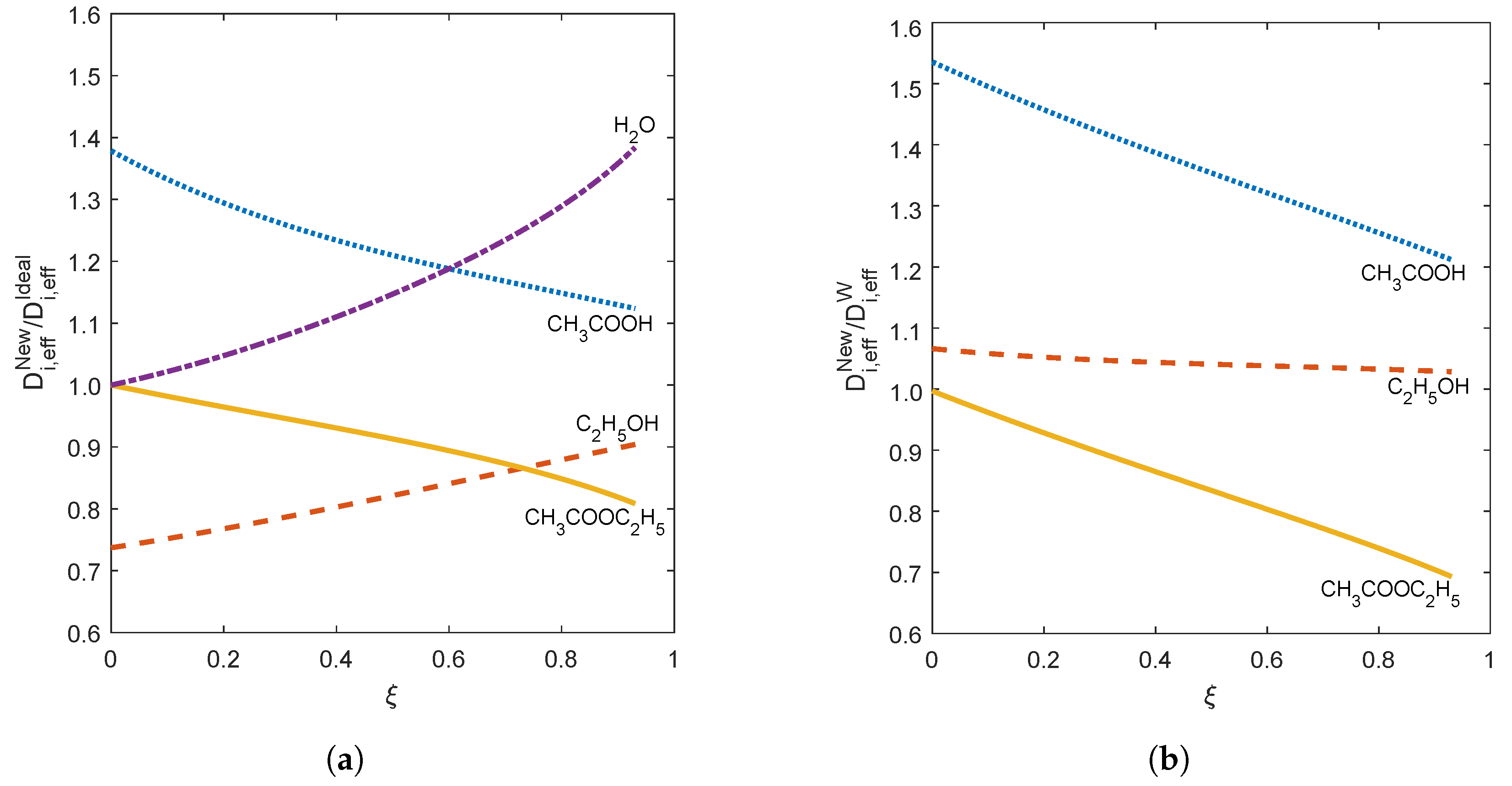
3.1. Liquid Phase Reaction: Ethyl Acetate Synthesis

Ethyl acetate may be synthesized via a Fisher esterification reaction of acetic acid and ethanol, as described by:

$$\mathrm{C}{\mathrm{H}}_3\mathrm{C}\mathrm{O}\mathrm{O}\mathrm{H}+\mathrm{C}{\mathrm{H}}_3\mathrm{C}{\mathrm{H}}_2\mathrm{O}\mathrm{H}\rightleftharpoons \mathrm{C}{\mathrm{H}}_3\mathrm{C}\mathrm{O}\mathrm{O}\mathrm{C}{\mathrm{H}}_2\mathrm{C}{\mathrm{H}}_3+{\mathrm{H}}_2\mathrm{O}$$

(21)

The number of moles of a component i in the mixture, $n_i$, is determined as function of the number of moles initially present, $n_{i0}$, the stoichiometric coefficient ${\nu }_i$ (with ${\nu }_i>0$ for products and ${\nu }_i<0$ for reactants), and the extent of reaction, $\xi$:

$$n_i=n_{i0}+{\nu }_i\xi$$

(22)

The mole fraction of component i can be computed by:

$$x_i=\frac{n_i}{n_T}=\frac{n_{i0}+{\nu }_i\xi }{n_{T0}}$$

(23)

where $n_T$ is the total number of moles, which remains constant throughout the reaction, $n_T=n_{T0}$, given that the sum of stoichiometric coefficients is zero for this particular reaction.

The goal for this reaction system is to calculate the effective diffusivity across a range of different compositions, from $\xi =0$ up to the maximum extent of reaction (at equilibrium), ${\xi }_{eq}$. The thermodynamic equilibrium constant, K, is described by:

$$K=\prod _{j=1}^n{a}_j^{{\nu }_j}=\prod _{j=1}^n{\left(x_j{\gamma }_j\right)}^{{\nu }_j}=\prod _{j=1}^n{x}_j^{{\nu }_j}\times \prod _{j=1}^n{\gamma }_j^{{\nu }_j}=K_x{K}_{\gamma }$$

(24)

where $a_j$ is the activity of component j, and $K_x$ and $K_{\gamma }$ are defined as $K_x\equiv {\prod }_{j=1}^n{x}_j^{{\nu }_j}$, $K_{\gamma }\equiv {\prod }_{j=1}^n{\gamma }_j^{{\nu }_j}$.

The group contribution method UNIFAC [8] is employed to estimate the activity coefficients (see the supporting information for further details). For any initial mixture composition the extent of reaction at equilibrium, at any given temperature, can be calculated numerically using the following iterative method:

• Obtain K or $K_x$ from the literature.
• Make an initial guess for the extent of reaction at equilibrium, ${\xi }_{eq}$.
• Compute equilibrium compositions ($x_{i,eq}$) for the assumed ${\xi }_{eq}$ (via Equation (23)) and then the respective activity coefficients, ${\gamma }_{i,eq}$.
• Calculate the equilibrium constant via Equation (24), $K^{calc}$.
• Compute the square of the deviation ${(K^{calc}-K)}^2$.
• Repeat steps 2–5 until the squared error is below a predetermined tolerance.

In order to apply the procedure described in Section 2.2, the molar diffusion fluxes ratio of each $ij$ pair of components must be known. This particular reaction constitutes a case of equimolar counterdiffusion (${\overline{N}}_T=0$), thus ${\overline{N}}_i={\overline{J}}_i$ and that ratio is simply given by:

$$\frac{{\overline{J}}_j}{{\overline{J}}_i}=\frac{{\overline{N}}_j}{{\overline{N}}_i}=\frac{{\nu }_j}{{\nu }_i}=\left\{\begin{array}{cc}1,\hfill & \mathrm{when}\mathit{i}\mathrm{and}\mathit{j}\mathrm{are}\mathrm{both}\mathrm{reactants}\mathrm{or}\mathrm{products}\hfill \\ -1,\hfill & \mathrm{when}\mathit{i}\mathrm{is}\mathrm{a}\mathrm{reactant}\mathrm{and}\mathit{j}\mathrm{is}\mathrm{a}\mathrm{product},\mathrm{or}\mathrm{vice-versa}\hfill \end{array}\right.$$

(25)

In the absence of experimental data the binary diffusion coefficients at infinite dilution and at the desired temperature can be estimated using the Wilke–Chang equation [9], and the liquid pure component viscosities by an empirical correlation from Perry’s Chemical Engineers’ Handbook [10] (see the supporting information).

For an initial equimolar mixture of reactants at 78 ${}^{°}$C (for which the experimental $K_x=2.67$ [11], the calculated $K_{\gamma }$ using UNIFAC model is $K_{\gamma }=3.72$, thus $K=9.94$) and total number of moles $n_{T0}=3$ mol, the extent of reaction at equilibrium is ${\xi }_{eq}=0.931$. The compositions at equilibrium are given in Table 1 along with the initial and final $D_{i,\mathrm{eff}}^{New}/D_{i,\mathrm{eff}}^{Model}$ ratios, which are used to assess the deviation of the new model relative to others. It should be noted that the model by Kubota et al. [5] is not listed since it yields the same result as the ideal equation for this particular reaction, given that ${\overline{N}}_T=0$. Moreover, apart from the new model and the ideal Bird et al. equation none of the other expressions allows for the determination of the effective diffusivity of the nth component (chosen as H₂O for this reaction). The graphical comparison in terms of $D_{i,\mathrm{eff}}^{New}/D_{i,\mathrm{eff}}^{Ideal}$ (with $D_{i,\mathrm{eff}}^{Ideal}$ given by Equation (6)) and $D_{i,\mathrm{eff}}^{New}/D_{i,\mathrm{eff}}^W$ (with $D_{i,\mathrm{eff}}^W$ given by Equation (5)) is illustrated in Figure 1.

Table 1. Effective diffusivities ratios $D_{i,\mathrm{eff}}^{New}/D_{i,\mathrm{eff}}^{Model}$ calculated at beginning ($\xi =0$; values enclosed in parentheses) and equilibrium (${\xi }_{eq}=0.931$) for an initial equimolar reactants mixture at 78 ${}^{°}$C using UNIFAC model to estimate the activity coefficients.

Component		CH3COOH	CH3CH2OH	CH3COOCH2CH3	H2O
Initial mole fractions		0.500	0.500	0.000	0.000
Calculated equilibrium mole fractions		0.190	0.190	0.310	0.310
Ratio	Reference Model
$D_{i,\mathrm{eff}}^{New}/D_{i,\mathrm{eff}}^{Ideal}$	Ideal (Bird et al.) [4], Equation (6)	(1.379) 1.124	(0.737) 0.904	(1.000) 0.809	(1.000) 1.384
$D_{i,\mathrm{eff}}^{New}/D_{i,\mathrm{eff}}^W$	Wilke [3], Equation (5)	(1.536) 1.212	(1.066) 1.029	(1.000) 0.694	-
$D_{i,\mathrm{eff}}^{New}/D_{i,\mathrm{eff}}^{BK}$	Burghardt and Krupiczka [2], Equation (8)	(1.254) 1.188	(0.793) 0.999	(1.0000) 0.650	-
$D_{i,\mathrm{eff}}^{New}/D_{i,\mathrm{eff}}^{Kato}$	Kato et al. [6], Equation (9)	(1.086) 1.048	(0.780) 1.039	(1.000) 1.625	-

Figure 1. Effective diffusivities ratios from $\xi =0$ up to equilibrium (${\xi }_{eq}=0.931$) for an initial equimolar reactants mixture at 78 ${}^{°}$C: (a) $D_{i,\mathrm{eff}}^{New}/D_{i,\mathrm{eff}}^{Ideal}$, and (b) $D_{i,\mathrm{eff}}^{New}/D_{i,\mathrm{eff}}^W$.

In Figure 1a, it can be seen that water is the component that exhibits the greatest effective diffusivity deviation from the ideal model (Equation (6)). This deviation increases rapidly from $\xi =0$ reaching 38.4% at equilibrium. Acetic acid starts with a 37.8% difference at the beginning of the reaction being reduced to 12.4% at equilibrium. In absolute terms, the average deviation across all components was 16.2%, with the average per component being 22.9% for acetic acid, −18.3% for ethanol, 15.1% for water, and −8.5% for ethyl acetate. Thus, neglecting the impact of the activity coefficients in the $[\Gamma ]$ matrix generates significant errors in the effective diffusivity computation of all components in this highly nonideal reaction system, as $D_{i,\mathrm{eff}}^{New}\ne D_{i,\mathrm{eff}}^{Ideal}$ for $\xi \ge 0$.

Comparing the new model with the Wilke equation, Figure 1b, acetic acid achieves the largest deviation (53.6% at $\xi =0$), followed by ethyl acetate (−30.6% at equilibrium), while the difference for ethanol remains quite low throughout the reaction. The average deviations are 36.8% for acetic acid, −15.3% for ethyl acetate, and 4.4% for ethanol. The overall average absolute deviation is equal to 18.8%.

3.2. High-Pressure Gas Phase Reaction: Methanol Synthesis

Two independent equations describing the reactions that occur during the catalytic gas phase methanol synthesis were considered. The first (I) is the methanol synthesis from carbon monoxide and the second (II) is the water–gas shift reaction [12]:

$$\begin{array}{c}\left(\mathrm{I}\right):\begin{array}{c}\hfill \mathrm{C}\mathrm{O}+2{\mathrm{H}}_2\rightleftharpoons \mathrm{C}{\mathrm{H}}_3\mathrm{O}\mathrm{H}\end{array}\end{array}$$

(26)

$$\begin{array}{c}\left(\mathrm{II}\right):\begin{array}{c}\hfill \mathrm{C}{\mathrm{O}}_2+{\mathrm{H}}_2\rightleftharpoons \mathrm{C}\mathrm{O}+{\mathrm{H}}_2\mathrm{O}\end{array}\end{array}$$

(27)

The equilibrium constants for reactions I and II are given by:

$$\begin{array}{c}{K}^I=\prod _{j=1}^n{a}_j^{{\nu }_j^I}=\prod _{j=1}^n{\left[\frac{{\widehat{\varphi }}_j{y}_{j}P}{P^{°}}\right]}^{{\nu }_j^I}=\frac{y_{C{H}_{3}OH}}{y_{CO}·y_{H_2}^2}\times \frac{{\widehat{\varphi }}_{C{H}_{3}OH}}{{\widehat{\varphi }}_{CO}·{\widehat{\varphi }}_{H_2}^2}\times {\left(\frac{P}{P^{°}}\right)}^{-2}\end{array}$$

(28)

$$\begin{array}{c}{K}^{II}=\frac{y_{H_{2}O}·y_{CO}}{y_{C{O}_2}·y_{H_2}}\times \frac{{\widehat{\varphi }}_{H_{2}O}·{\widehat{\varphi }}_{CO}}{{\widehat{\varphi }}_{C{O}_2}·{\widehat{\varphi }}_{H_2}}\end{array}$$

(29)

where ${\nu }_j^I$ is the stoichiometric coefficient of component j in reaction I, $y_j$ is the mole fraction of j in the gas phase, ${\widehat{\varphi }}_j$ is its fugacity coefficient, P is the system pressure, and $P^{°}$ is the standard pressure (1 bar).

Several equilibrium expressions can be found in the literature. According to Chinchen et al. [12], the expressions by Cherednichenko (Equation (30)) and Besset (Equation (31)) [13] have been successfully employed in the analysis of a commercial methanol synthesis plant and thus were chosen in the present work. In terms of thermodynamic constants as function of temperature, they are given by:

$$\begin{array}{c}{K}^I=9.740\times {10}^{-1}\times exp\left(21.225+\frac{9143.6}{T}-7.492lnT+4.076\times {10}^{-3}T-7.161\times {10}^{-8}{T}^2\right)\end{array}$$

(30)

$$\begin{array}{c}{K}^{II}=exp\left(13.148-\frac{5639.5}{T}-1.077lnT-5.44\times {10}^{-4}T+1.125\times {10}^{-7}{T}^2+\frac{49170}{T^2}\right)\end{array}$$

(31)

where T is the absolute temperature (in K). It has been reported that over copper-based catalysts, the water–gas shift reaction is approximately 2–3 orders of magnitude faster than methanol synthesis [14]. Therefore, it is possible to assume that reaction II reaches equilibrium instantaneously.

Given the presence of two reactions, the number of moles of an arbitrary component i depends on the extents of both reactions, ${\xi }^I$ and ${\xi }^{II}={\xi }_{eq}^{II}$, by:

$$d{n}_i={\nu }_i^{I}d{\xi }^I+{\nu }_i^{II}d{\xi }_{eq}^{II}$$

(32)

where ${\nu }_i^I$ and ${\nu }_i^{II}$ represent the stoichiometric coefficients of species i in reactions I and II, respectively. The total number of moles in the mixture is given by:

$$n_T=\sum _{j=1}^n{n}_j=n_{T0}-2{\xi }^I$$

(33)

Using Equation (33) and the integrated form of Equation (32), the mole fraction of component i can then be calculated by:

$$y_i=\frac{n_i}{n_T}=\frac{n_{i0}+{\nu }_i^I{\xi }^I+{\nu }_i^{II}{\xi }_{eq}^{II}}{n_{T0}-2{\xi }^I}$$

(34)

Because there are two reactions the method for determining the molar diffusion fluxes ratio is more complex. Using CO as reference component (since it takes part in both reactions) Equation (35) can be written to compute the molar diffusion fluxes ratio, ${\overline{J}}_j/{\overline{J}}_i$.

$$\frac{{\overline{J}}_j}{{\overline{J}}_i}=\frac{{\overline{N}}_j-y_j{\overline{N}}_T}{{\overline{N}}_i-y_i{\overline{N}}_T}=\frac{{\overline{N}}_j/{\overline{N}}_{CO}-y_j{\overline{N}}_T/{\overline{N}}_{CO}}{{\overline{N}}_i/{\overline{N}}_{CO}-y_i{\overline{N}}_T/{\overline{N}}_{CO}}$$

(35)

Inside the catalyst pellet the rate of disappearance of a species due to the chemical reactions is proportional to the flux of said species, thus:

$$\frac{{\overline{N}}_i}{{\overline{N}}_{CO}}=\frac{r_i}{r_{CO}}=\frac{d{n}_i}{d{n}_{CO}}=\frac{{\nu }_i^{I}d{\xi }^I+{\nu }_i^{II}d{\xi }_{eq}^{II}}{-d{\xi }^I+d{\xi }_{eq}^{II}}=\frac{{\nu }_i^I+{\nu }_i^{II}\frac{d{\xi }_{eq}^{II}}{d{\xi }^I}}{-1+\frac{d{\xi }_{eq}^{II}}{d{\xi }^I}}$$

(36)

where $r_i$ and $r_{CO}$ are the reaction rates of components i and CO, respectively. The ${\overline{N}}_T/{\overline{N}}_{CO}$ ratio, which also must be determined in order to apply Equation (35), is simply obtained by summing up Equation (36) over all species.

$$\frac{{\overline{N}}_T}{{\overline{N}}_{CO}}=\sum _{j=1}^n\frac{{\overline{N}}_j}{{\overline{N}}_{CO}}=\frac{-2}{-1+\frac{d{\xi }_{eq}^{II}}{d{\xi }^I}}$$

(37)

A specific procedure can be developed to determine the ratios ${\overline{J}}_j/{\overline{J}}_i$ for this reaction system before the effective diffusivities can be evaluated:

• For a given temperature, pressure and initial mixture composition calculate the final values of the extents of reaction, ${\xi }_{eq}^I$ and ${\xi }_{eq}^{II}$, as described in Section 3.1.
• Calculate the corresponding ${\xi }_{eq}^{II}$ for each ${\xi }^I$ in the span of $[0,{\xi }_{eq}^I]$ by solving Equation (38) numerically:

  $$\frac{K^{II,calc}}{K^{II}}-1=0\iff \frac{y_{H_{2}O}·y_{CO}}{y_{C{O}_2}·y_{H_2}}\times \frac{{\widehat{\varphi }}_{H_{2}O}·{\widehat{\varphi }}_{CO}}{{\widehat{\varphi }}_{C{O}_2}·{\widehat{\varphi }}_{H_2}}\times \frac{1}{K^{II}}-1=0$$

  (38)
  Since the mole fractions are functions of the extent of reactions (Equation (34)), Equation (38) is implicit in ${\xi }_{eq}^{II}$. The fugacity coefficients are functions of mole fractions, temperature, and pressure, and $K^{II}$ is given by Equation (31).
• Once ${\xi }_{eq}^{II}$ has been determined as function of ${\xi }^I$ (over $[0,{\xi }_{eq}^I]$), the derivatives $\frac{d{\xi }_{eq}^{II}}{d{\xi }^I}$ can be calculated numerically using finite differences, for instance.
• The fluxes ratios ${\overline{N}}_i/{\overline{N}}_{CO}$ can be determined via Equation (36) and then replaced in Equation (35) to obtain the molar diffusion fluxes ratios ${\overline{J}}_j/{\overline{J}}_i$.
• The effective diffusivities can then be evaluated following the procedure delineated in Section 3.1.

The binary diffusion coefficients at infinite dilution are estimated using the correlation developed by Riazi and Whitson [9], which requires: (1) viscosity data for the components at low pressure and high pressure, that can be estimated by Stiel and Thodos [15] and Jossi et al. [16] equations; (2) binary diffusion coefficients at low pressure, estimated with the Fuller-Giddins-Schettler equation [9]; (3) high pressure and low pressure density of all pure components, evaluated using an equation of state (EoS). Auxiliary equations can be found in the supporting information.

The equations of state used in the present work are Peng–Robinson (PR) and PC-SAFT. The greatest limitation of the former is its reliance on the $k_{ij}$ binary interaction parameters, which are adjusted to experimental data. In the absence of such data the embodied $k_{ij}$ are assumed to be equal to 0 for each pair of components. Thus, the results may deviate significantly from reality, especially in the presence of polar molecules that can establish hydrogen bonds, such as CH₃OH and H₂O. In order to account for such limitations effective diffusivities are also evaluated with PC-SAFT EoS. Although this equation can also incorporate binary interaction parameters fitted to experimental data, due to its theoretical foundations in statistical mechanics it tends to be highly reliable in its predictive capability as shown for several binary systems in the work by Gross and Sadowski [17].

The effective diffusivities are calculated for the system at 573.15 K and 10 MPa with 100 moles initially present in the mixture ($n_{T0}=100$ mol). The initial mole fractions of the mixture are taken from Cappelli et al. [18] representing a typical feed for a methanol synthesis reactor operating at high pressure. After normalization to exclude N₂ they are: 12.14% CO, 0.12% CH₃OH, 70.94% H₂, 0.16% H₂O, 14.90% CH₄ (inert) and 1.74% CO₂. Fugacity coefficients from PR EoS are computed with a self-developed program. The code developed by Ángel Martín is used to compute fugacity coefficients with PC-SAFT EoS [19,20].

Table 2 and Table 3 present effective diffusivity ratios of the new model relative to all models using PR EoS and PC-SAFT EoS, respectively, at initial and equilibrium compositions. The ratios $D_{i,\mathrm{eff}}^{New}/D_{i,\mathrm{eff}}^{Ideal}$ and $D_{i,\mathrm{eff}}^{New}/D_{i,\mathrm{eff}}^W$ as function of ${\xi }^I$ are shown in Figure 2 and Figure 3, respectively. The results in Figure 3 exclude methane (due to ratios above 6 obscuring the differences among the remaining components) and carbon dioxide (chosen as component n and thus unable to be computed by Wilke equation).

Table 2. Effective diffusivities ratios $D_{i,\mathrm{eff}}^{New}/D_{i,\mathrm{eff}}^{Model}$ calculated at beginning (${\xi }^I=0$; ${\xi }_{eq}^{II}=0.1014$; values enclosed in parentheses) and equilibrium (${\xi }_{eq}^I=7.5068$; ${\xi }_{eq}^{II}=0.2994$), using Peng–Robinson EoS at 573.15 K and 10 MPa.

Component		CO	CH3OH	H2	H2O	CH4	CO2
Initial mole fractions		0.1224	0.0012	0.7084	0.0026	0.1490	0.0164
Calculated equilibrium mole fractions		0.0580	0.0897	0.6545	0.0054	0.1753	0.0170
Ratio	Reference Model
$D_{i,\mathrm{eff}}^{New}/D_{i,\mathrm{eff}}^{Ideal}$	Ideal (Bird et al.) [4], Equation (6)	(1.011) 0.9961	(0.9994) 0.9612	(0.9436) 0.8708	(0.8817) 0.9465	(0.5557) 0.5118	(1.2423) 1.0446
$D_{i,\mathrm{eff}}^{New}/D_{i,\mathrm{eff}}^W$	Wilke [3], Equation (5)	(0.6340) 0.8241	(0.9992) 0.9414	(0.6826) 0.6808	(1.3416) 1.1576	(5.2983) 10.3318	-
$D_{i,\mathrm{eff}}^{New}/D_{i,\mathrm{eff}}^K$	Kubota et al. [5], Equation (7)	(0.7529) 0.8717	(1.0018) 1.1376	(0.2793) 0.3119	(1.2530) 1.0454	-	-
$D_{i,\mathrm{eff}}^{New}/D_{i,\mathrm{eff}}^{BK}$	Burghardt and Krupiczka [2], Equation (8)	(0.8063) 0.8912	(1.0015) 1.1119	(0.7403) 0.6922	(1.3480) 1.1658	(6.8448) 12.9857	-
$D_{i,\mathrm{eff}}^{New}/D_{i,\mathrm{eff}}^{Kato}$	Kato et al. [6], Equation (9)	(0.7775) 0.8782	(1.0023) 1.1822	(0.7162) 0.7011	(1.3473) 1.1656	(6.7167) 12.7846	-

Table 3. Effective diffusivities ratios $D_{i,\mathrm{eff}}^{New}/D_{i,\mathrm{eff}}^{Model}$ calculated at beginning (${\xi }^I=0$; ${\xi }_{eq}^{II}=0.0935$; values enclosed in parentheses) and equilibrium (${\xi }_{eq}^I=7.3797$; ${\xi }_{eq}^{II}=0.2894$) using PC-SAFT EoS at 573.15 K and 10 MPa.

Component		CO	CH3OH	H2	H2O	CH4	CO2
Initial mole fractions		0.1223	0.0012	0.7085	0.0025	0.1490	0.0165
Calculated equilibrium mole fractions		0.0592	0.0880	0.6557	0.0053	0.1748	0.0170
Ratio	Reference Model
$D_{i,\mathrm{eff}}^{New}/D_{i,\mathrm{eff}}^{Ideal}$	Ideal (Bird et al.) [4], Equation (6)	(1.0100) 1.0007	(0.9994) 0.9569	(0.9424) 0.8695	(0.8339) 0.9152	(0.7685) 0.8996	(1.2238) 1.0319
$D_{i,\mathrm{eff}}^{New}/D_{i,\mathrm{eff}}^W$	Wilke [3], Equation (5)	(0.6525) 0.8441	(1.0330) 0.9738	(0.6962) 0.6976	(1.2542) 1.1845	(4.6316) 8.1610	-
$D_{i,\mathrm{eff}}^{New}/D_{i,\mathrm{eff}}^K$	Kubota et al. [5], Equation (7)	(0.7749) 0.8963	(1.0357) 1.1687	(0.2848) 0.3231	(1.1762) 1.1586	-	-
$D_{i,\mathrm{eff}}^{New}/D_{i,\mathrm{eff}}^{BK}$	Burghardt and Krupiczka [2], Equation (8)	(0.8298) 0.9148	(1.0354) 1.1466	(0.7551) 0.7100	(1.2599) 1.1928	(5.9837) 10.2637	-
$D_{i,\mathrm{eff}}^{New}/D_{i,\mathrm{eff}}^{Kato}$	Kato et al. [6], Equation (9)	(0.7943) 0.8986	(1.0362) 1.2237	(0.7450) 0.7306	(1.2591) 1.1923	(5.8233) 10.0110	-

Figure 2. Effective diffusivities ratios $D_{i,\mathrm{eff}}^{New}/D_{i,\mathrm{eff}}^{Ideal}$ as function of extent of reaction I, up to equilibrium, using (a) Peng–Robinson EoS (${\xi }_{eq}^I=7.5068$; ${\xi }_{eq}^{II}=0.2994$), and (b) PC-SAFT EoS (${\xi }_{eq}^I=7.3797$; ${\xi }_{eq}^{II}=0.2894$).

Figure 3. Effective diffusivities ratios $D_{i,\mathrm{eff}}^{New}/D_{i,\mathrm{eff}}^W$ as function of extent of reaction I, up to equilibrium, using (a) Peng–Robinson EoS (${\xi }_{eq}^I=7.5068$; ${\xi }_{eq}^{II}=0.2994$), and (b) PC-SAFT EoS (${\xi }_{eq}^I=7.3797$; ${\xi }_{eq}^{II}=0.2894$).

A more direct comparison between the results achieved by the two equations of state can be seen in Table 4, which shows $D_{i,\mathrm{eff},\mathrm{PR}}^{New}/D_{i,\mathrm{eff},\mathrm{PC}-\mathrm{SAFT}}^{New}$ at ${\xi }^I=0$ and ${\xi }^I=7.3797$. Note that the extent of reaction II and mixture composition will differ slightly due to differences between the PR and PC-SAFT fugacity coefficients, which are involved in the calculation of ${\xi }_{eq}^{II}$. The fugacity coefficients calculated with PR EoS and PC-SAFT EoS for all components are shown in Figure 4.

Table 4. Effective diffusivities ratios $D_{i,\mathrm{eff},\mathrm{PR}}^{New}/D_{i,\mathrm{eff},\mathrm{PC-SAFT}}^{New}$ at ${\xi }^I=0$ (values enclosed in parentheses) and ${\xi }^I=7.3797$, at 573.15 K and 10 MPa.

Component	CO	CH3OH	H2	H2O	CH4	CO2
Initial mole fractions (PR)	0.1224	0.0012	0.7084	0.0026	0.1490	0.0164
Initial mole fractions (PC-SAFT)	0.1223	0.0012	0.7085	0.0025	0.1490	0.0165
Calculated final mole fractions (PR)	0.0593	0.0880	0.6557	0.0053	0.1748	0.0170
Calculated final mole fractions (PC-SAFT)	0.0592	0.0880	0.6557	0.0053	0.1748	0.0170
$D_{i,\mathrm{eff},\mathrm{PR}}^{New}/D_{i,\mathrm{eff},\mathrm{PC-SAFT}}^{New}$	(0.9716) 0.9722	(0.9672) 0.9678	(0.9805) 0.9754	(1.0697) 0.9796	(1.1438) 1.2379	(0.9140) 0.9343

Figure 4. Fugacity coefficients as function of extent of reaction I computed with (a) Peng–Robinson EoS and (b) PC-SAFT EoS.

Comparing the $D_{i,\mathrm{eff}}^{New}/D_{i,\mathrm{eff}}^{Ideal}$ ratios (Figure 2), the maximum deviation using PR EoS (Figure 2a) is for CH₄ at equilibrium (−48.8%) and in second place for CO₂ at the beginning of the reaction (24.2%). For PC-SAFT EoS (Figure 2b), the largest and second largest deviations are for the same components, although with lower deviations for CH₄ (−23.1%) and CO₂ (22.4%) both at ${\xi }^I=0$. Other components exhibit significant differences (above 10%) with the exception of CO, whose deviation is less than 1% in magnitude. Thus, only the results for CO are in good agreement with the ideal model for this reaction system at the aforementioned temperature and pressure conditions. The average absolute deviation across all components is 13.1% and 9.0% for PR EoS and PC-SAFT EoS, respectively, with the largest average deviation being for CH₄ (PR EoS: −45.8%, PC-SAFT EoS: −18.2%), followed by CO₂ (PR EoS: 13.0%, PC-SAFT EoS: 11.1%).

With regards to the $D_{i,\mathrm{eff}}^{New}/D_{i,\mathrm{eff}}^W$ ratios (Figure 3), when using the PR EoS (Figure 3a and Table 2), the maximum deviation is also attributed to CH₄, which reaches 933.8% at ${\xi }^I={\xi }_{eq}^I$, followed by CO with −36.6% at ${\xi }^I=0$. The component that exhibits the lowest ratio is methanol, reaching a maximum of 5.9%. The same pattern is observed with PC-SAFT EoS (Figure 3b and Table 3) but in lower percentages (716.1% for CH₄, −34.8% for CO). Although the CO deviation reduces as the first reaction approaches equilibrium, that of H₂ remains high throughout the entire range of ${\xi }^I$ resulting in a higher average deviation for this component (PR EoS: −32.1%, PC-SAFT EoS: −30.5%) than for CO. However, once again the highest average deviation is for CH₄ (PR EoS: 604.6%, PC-SAFT EoS: 494.2%). The overall absolute averages are 138.3% and 114.8% for PR EoS and PC-SAFT EoS, respectively, with the numbers being skewed toward high values due to CH₄.

Analyzing Table 4 one can observe a large difference between the predicted effective diffusivities obtained with PR EoS and PC-SAFT EoS for CH₄, while slight deviations are achieved for CO, CH₃OH, and H₂. The $D_{i,\mathrm{eff},\mathrm{PR}}^{New}/D_{i,\mathrm{eff},\mathrm{PC-SAFT}}^{New}$ ratio for H₂O decreases as the extent of reaction increases, exhibiting a maximum value of 7.0% at ${\xi }^I=0$. Such deviations are likely caused by the presence of dipole-dipole and hydrogen bonding interactions that are not accurately accounted by the PR EoS. Figure 4 emphasizes the distinct performance of both equations of state since very different fugacity coefficients are calculated for water and ethanol, notwithstanding their similar trends along reaction progression.

4. Conclusions

A new model for multicomponent effective diffusivity has been developed taking account of the nonideal behavior in compressed gas and liquid mixtures by incorporating fugacity or activity coefficients. It can be used to calculate the effective diffusivity of all species, including the nth component, and it does not have any underlying restrictive assumption such as equimolar counterdiffusion, unimolecular diffusion or infinite dilution. It is demonstrated that when nonidealities are ignored the new model results in the well known equation of Bird et al., which is the exact analytical solution for ideal mixtures. The application of the new model is illustrated for two catalytic reactions, the liquid phase synthesis of ethyl acetate and the gas phase synthesis of methanol, and in both cases the importance of accounting for the nonideal behavior of the mixture is enlightened. From the models adopted for comparison the worst results based on the overall absolute average deviation are achieved by the Wilke (for ethyl acetate synthesis) and Kubota et al. equations.

References

- Aris, R. The Mathematical Theory of Diffusion and Reaction in Permeable Catalysts. Volume 1: The Theory of the Steady State, 1st ed.; Oxford University Press: Oxford, UK, 1975. [Google Scholar]
- Taylor, R.; Krishna, R. Multicomponent Mass Transfer; Wiley: New York, NY, USA, 1993. [Google Scholar]
- Wilke, C.R. Diffusional Properties of Multicomponent Gases. Chem. Eng. Prog. 1950, 46, 95–104. [Google Scholar]
- Bird, R.B.; Stewart, W.E.; Lightfoot, E.N. Transport Phenomena; John Wiley and Sons: New York, NY, USA, 1960. [Google Scholar]
- Kubota, H.; Yamanaka, Y.; Lana, I.G.D. Effective Diffusivity of Multi-Component Gaseous Reaction System: Application to Evaluate Catalyst Effectiveness Factor. J. Chem. Eng. Jpn. 1969, 2, 71–75. [Google Scholar] [CrossRef]
- Kato, S.; Inazumi, H.; Suzuki, S. Mass transfer in a ternary gaseous phase. Int. Chem. Eng 1981, 21, 443–452. [Google Scholar]
- Vignes, A. Diffusion in Binary Solutions. Variation of Diffusion Coefficient with Composition. Ind. Eng. Chem. Fundam. 1966, 5, 189–199. [Google Scholar] [CrossRef]
- Elliott, J.R.; Lira, C.T. Introductory Chemical Engineering Thermodynamics, 2nd ed.; Prentice Hall: Upper Saddle River, NJ, USA, 2012. [Google Scholar]
- Poling, B.E.; Prausnitz, J.M.; O’Connell, J.P. The Properties of Gases and Liquids, 5th ed.; McGraw-Hill: New York, NY, USA, 2001. [Google Scholar]
- Green, D.W.; Southard, M.Z. Perry’s Chemical Engineers’ Handbook, 9th ed.; McGraw Hill Education: New York, NY, USA, 2019. [Google Scholar]
- Antunes, B.M.; Cardoso, S.P.; Silva, C.M.; Portugal, I. Kinetics of Ethyl Acetate Synthesis Catalyzed by Acidic Resins. J. Chem. Educ. 2011, 88, 1178–1181. [Google Scholar] [CrossRef]
- Chinchen, G.; Denny, P.; Jennings, J.; Spencer, M.; Waugh, K. Synthesis of Methanol. Appl. Catal. 1988, 36, 1–65. [Google Scholar] [CrossRef]
- Chang, T.; Rousseau, R.W.; Kilpatrick, P.K. Methanol Synthesis Reactions: Calculations of Equilibrium Conversions Using Equations of State. Ind. Eng. Chem. Process. Des. Dev. 1986, 25, 477–481. [Google Scholar] [CrossRef]
- Yang, Y.; Evans, J.; Rodriguez, J.A.; White, M.G.; Liu, P. Fundamental Studies of Methanol Synthesis from CO2 Hydrogenation on Cu(111), Cu Clusters, and Cu/ZnO(000). Phys. Chem. Chem. Phys. 2010, 12, 9909. [Google Scholar] [CrossRef] [PubMed]
- Stiel, L.I.; Thodos, G. The Viscosity of Polar Gases at Normal Pressures. AIChE J. 1962, 8, 229–232. [Google Scholar] [CrossRef]
- Jossi, J.A.; Stiel, L.I.; Thodos, G. The Viscosity of Pure Substances in the Dense Gaseous and Liquid Phases. AIChE J. 1962, 8, 59–63. [Google Scholar] [CrossRef]
- Gross, J.; Sadowski, G. Perturbed-Chain SAFT: An Equation of State Based on a Perturbation Theory for Chain Molecules. Ind. Eng. Chem. Res. 2001, 40, 1244–1260. [Google Scholar] [CrossRef]
- Cappelli, A.; Collina, A.; Dente, M. Mathematical Model for Simulating Behavior of Fauser-Montecatini Industrial Reactors for Methanol Synthesis. Ind. Eng. Chem. Process. Des. Dev. 1972, 11, 184–190. [Google Scholar] [CrossRef]
- Ángel, M. [Open Source Software] Equations of State. Available online: https://hpp.uva.es/open-source-software-eos/ (accessed on 8 August 2022).
- Martín, Á.; Bermejo, M.D.; Mato, F.A.; Cocero, M.J. Teaching Advanced Equations of State in Applied Thermodynamics Courses Using Open Source Programs. Educ. Chem. Eng. 2011, 6, e114–e121. [Google Scholar] [CrossRef]
- Chapman, W.G.; Gubbins, K.E.; Jackson, G.; Radosz, M. New reference equation of state for associating liquids. Ind. Eng. Chem. Res. 1990, 29, 1709–1721. [Google Scholar] [CrossRef]
- Crespo, E.A.; Coutinho, J.A.P. A Statistical Associating Fluid Theory Perspective of the Modeling of Compounds Containing Ethylene Oxide Groups. Ind. Eng. Chem. 2019, 58, 3562–3582. [Google Scholar] [CrossRef]
- Lee, B.-S.; Kim, K.-C. Liquid–Liquid Equilibrium of Associating Fluid Mixtures Using Perturbed-Hard-Sphere-Chain Equation of State Combined with the Association Model. Ind. Eng. Chem. Res. 2015, 54, 540–549. [Google Scholar] [CrossRef]
- Khare, N.P.; Lucas, B.; Seavey, K.C.; Liu, Y.A.; Sirohi, A.; Ramanathan, S.; Lingard, S.; Song, Y.; Chen, C.C. Steady-State and Dynamic Modeling of Gas-Phase Polypropylene Processes Using Stirred-Bed Reactors. Ind. Eng. Chem. Res. 2004, 43, 884–900. [Google Scholar] [CrossRef]
- Martín, Á.; Pham, H.M.; Kilzer, A.; Kareth, S.; Weidner, E. Phase equilibria of carbon dioxide+ poly ethylene glycol+water mixtures at high pressure: Measurements and modelling. Fluid Phase Equilibria 2009, 286, 162–169. [Google Scholar] [CrossRef]
Publisher’s Note: MDPI stays neutral with regard to jurisdictional claims in published maps and institutional affiliations. |
© 2022 by the authors. Licensee MDPI, Basel, Switzerland. This article is an open access article distributed under the terms and conditions of the Creative Commons Attribution (CC BY) license (https://creativecommons.org/licenses/by/4.0/).