Article

Three-Dimensional Dynamic Formation of Second-Order Multi-Agent System Based on Rigid Graphs

1
Network Management Center of Network Department, China Mobile Communications Group Shanxi Co., Ltd., Taiyuan 030032, China
2
State Key Laboratory of Dynamic Measurement Technology, North University of China, Taiyuan 030051, China
*
Author to whom correspondence should be addressed.
These authors contributed equally to this work.
Processes 2022, 10(10), 1961; https://doi.org/10.3390/pr10101961
Submission received: 20 August 2022 / Revised: 9 September 2022 / Accepted: 25 September 2022 / Published: 28 September 2022
(This article belongs to the Special Issue Advanced Processes Creating New Technologies in Tomorrow's Industry)

Abstract

:
This paper studies the dynamic formation control of second-order multi-agent systems (MASs) in three-dimensional space based on the distance control approach. A rigid graph represents the communication topology between agents to improve the system’s robustness and stability and avoid collisions and deformations during formation operation. A distributed control strategy based on the relative states among neighbors is designed for each agent to achieve formation and formation maintenance under arbitrary initial conditions. The Lyapunov function, an error function of potential and kinetic energy, is constructed by rigid graph theory and a second-order integrator model. The decreasing of the Lyapunov function is proven by Barbalat’s theory, further indicating that the system is asymptotically stable. A second-order MAS composed of nine agents is constructed, and the dynamic scaling of rigid formations in 3D space is achieved through simulation to verify the effectiveness of the controller and the correctness of the theory.

1. Introduction

Agents are dynamic systems that can perceive their environment and react appropriately to it. In contrast to static circumstances with no motion, Animasaun et al. [1] described a dynamic system as a system or process in which motion occurs or one that involves active forces, such as underwater vehicles and unmanned vehicles. Compared with a single agent’s number of tasks and efficiency, the multi-agent system (MAS) can efficiently perform the specified functions through specific organizational rules and information interaction protocols between agents. The consensus is fundamental in the study of MAS, and many cooperative tasks, such as swarming, flocking, formation, and tracking, are fully under consensus. However, formation control can achieve more desirable results in many practical applications, such as cooperative search, cooperative transportation, and combat reconnaissance.
Specifically, a control method that completes information exchange through a communication network between neighboring agents and without global information is called distributed formation control. This control method reduces the quantity of information processing considerably during operation and applies to combat scenarios where the communication environment is limited and GPS signals cannot be located, making the MAS highly autonomous [2,3]. For example, when autonomous underwater vehicles (AUV) are used for path planning and seafloor exploration, they need to acquire large-area images of the seafloor. In some cases, the global positioning system (GPS) signal of the underwater vehicles is limited and cannot obtain all the companion position information [4,5]. After forming a designated stratum through distributed formation control, each captures the corresponding waters and finally stitches together the images obtained by each AUV to obtain a complete topographic map of the seafloor. It is necessary to maintain a distance during the movement of each submersible to avoid a collision. The existing methods can be divided into formation control methods based on position, displacements, and distances according to the variables. The based distance formation control method, in particular, requires each agent to communicate with its neighbors via its carrying sensors and communication network to convey each one’s position, angle, and relative displacement in the local coordinate system. Through designing control protocols, predefined angles and distances are generated between agents to accomplish specific collaborative tasks.
Graph theory is a commonly used tool to solve issues related to MASs, and rigid graphs play an essential role in distance-based formation control. In 2002, Olfati-Saber [6] first employed rigid graph theory in the formation control of MASs and combined multiple smaller-scale rigid graphs into larger-scale rigid graphs by specific rules. Most of the early research on formation control treated the agents as masses and analyzed formation control based on single integrators [7,8]. Refs. [9,10] realized formation acquisition and formation motion of MASs, respectively, but the single integrator model has apparent limitations when considering the individual dynamics of agents. The formation control of multi-agent systems was studied in [11] using a first-order integrator model and a second-order integrator model and rigid graph theory, respectively. The formation acquisition and dynamic control are investigated in [12] utilizing the second integrator model for realizing a formation’s overall movement. In the literature [13], a distributed control law is designed based on rigid graph theory and the second-order integrator model to gradually stabilize the formation with minimum rigidity. Kwang-Kyo Oh [14] et al. exploited the properties of gradient systems to prove that single and double integrator models are also locally asymptotically stable in n-dimensional space in the presence of non-infinitesimal rigidity. For the formation complexity of the formed formations, the previous studies primarily focused on simple formations of systems, such as triangles [15] and rectangles, considering the nonlinear terms of rigid systems. Later, scholars studied the robustness of formations more comprehensively. Refs. [16,17] investigated tetrahedral formations of MASs in three dimensions, compared with the former, which derived the effect of a pre-determined distance on the rigid formation motion. A global asymptotic stabilization and avoidance scheme is proposed in [18] using a distance-based formation control method. A distributed control law based on the amount of distance was designed in [19] to accomplish formation acquisition and target tracking for a single integrator model. After this, an observer was introduced in [20] to design a distance-based control law for the non-complete kinematic model, which eventually achieves formation control and target tracking of the cart. In the above studies, the expected formations were primarily static, i.e., the distance between agents was time-independent. However, in some practical applications, the formation needs to be adjusted according to the actual situation. For example, when a narrow passage is encountered in the process of AUV formation for seafloor exploration, the formation can be contracted proportionally, which ensures that the rigidity of the formation is not destroyed and it achieves collision avoidance for the members within the system. Previously, many scholars studied the MAS dynamic formation control problem by a first-order integrator model, e.g., refs. [8,21,22], after which, considering that most of the objects in real life move with external forces, a more practical application-oriented model was adopted: the second-order integrator model. By changing the external force on the object, we change the acceleration of the object, thus affecting the velocity and displacement of the object. The second-order integrator model is conceived as a mass point, whose acceleration can be changed by the action of external forces. Therefore, this model can be considered as a simple omnidirectional robot dynamics model. In [14,23], the distance between the second-order integrator models is described using the Hamiltonian energy system, and asymptotic stabilization is achieved under the gradient control law.
This paper investigates rigid dynamic formation in three-dimensional space thoroughly by distance-based formation control and designs a formation control law for MAS controlled by a double integrator. In the process of dynamic formation realization, the following two main issues are considered: the formation of rigid formations and the dynamic transformation and collision avoidance of rigid formations. The main contributions of this paper are as follows. First, a distance-based rigid formation control method is adopted for avoiding internal collisions during the formation movement. Second, we design the appropriate speed of movement and rotation speed within the formation to achieve the encircling movement of the formation.
The rest of this article is structured as follows. Section 2 introduces the basic concepts and symbolic meaning of rigid graph theory. The second-order integrator control model is presented, and the MAS in three-dimensional space is modeled, in Section 3. The distance-based formation control law and the formation motion equations are designed in Section 4. Simulation results are presented to achieve dynamic formation in Section 5. The conclusion of this article is presented in Section 6.

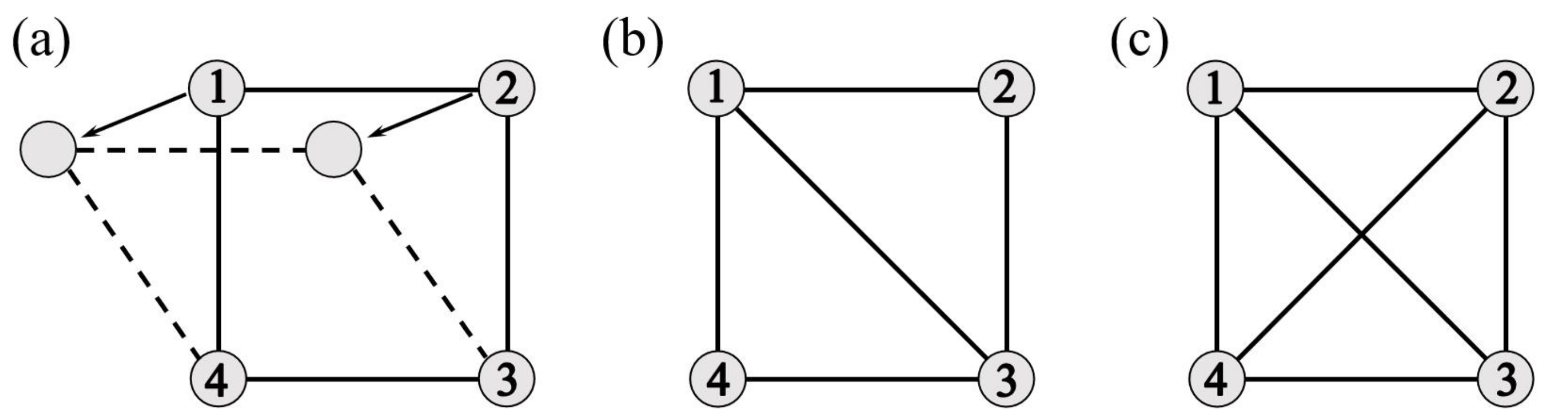
2. Notations and Basic Concepts

The undirected graph is denoted by G = V , E , A ; V = 1 , 2 , . . . , n is the set of points. The element number of V matches the number of agents in MAS. The elements in E V × V denote the communication edges between n agents, and the number of edges determines whether or not the undirected graph G is rigid. For an undirected graph, the adjacency matrix A = [ a i j ] is a symmetric matrix. The neighbors of i-th agent are represented by N i ( E ) = { j V ( i , j ) E } . If ( i , j ) E , the adjacency matrix is a i j = a j i = 1 ; otherwise, it is a i j = 0 . It is important to note that a i i = 0 . Suppose that the i-th agent’s position is indicated by the symbol X i R m , where X = X 1 , X 2 , . . . , X n R n m . X ^ i j = X i X j is set to represent the position of two agents in relation to one another. F = G , X represents an undirected graph G at coordinates X. Define an edge function Ψ G X : R m n R l , with l indicating the number of edges in the graph. It is worth noting that the side function Ψ G X is invariant when the formation maintains distance motion.
Ψ G X = . . . , X ^ i j 2 , . . . T , i , j E
where X ^ i j represents the Euclidean parametrization of X ^ i j . For two undirected graphs of frames F 1 = G , X 1 and F 2 = G , X 2 with G = { V , E , A } , F 1 and F 2 are called equivalent if X 1 i X 1 j = X 2 i X 2 j for i , j E [24], i.e., the side functions Ψ G X in (1) are equivalent. F 1 and F 2 are called congruent if X 1 i X 1 j = X 2 i X 2 j for i , j E for i , j V , i.e., the distances between any two corresponding points (including unconnected points) in F 1 and F 2 are the same. Therefore, the strength of congruent is greater than equivalent. The set of all frameworks that are isomorphic to F is denoted by the symbol I s o F . It is important that congruency is a sufficient and unnecessary condition for equivalence, and the converse is incorrect.
Lemma 1.
There exists a mapping relation H : R n R n such that
H X 1 H X 2 = X 1 X 2 , X 1 , X 2 R n
where H means translation or rotation of the vector x 1 x 2 .
Rigid graph theory plays an important role in distance-based formation control, because rigidity can provide distance constraints during formation movement so that the formation can rotate and translate only as a whole, avoiding unnecessary collisions within the formation. Rigidity is divided into global rigidity, infinitesimal rigidity, and minimum rigidity. A brief description of the rigid framework follows.
Minimum rigidity [25] is the threshold of rigidity; eliminating any one edge will make the graph unstable, as shown in Figure 1b. No flip occurs inside the global rigid graph, which is the most stable structure, as shown in Figure 1c, while Figure 1a is non-rigid.
Definition 1
([19,20]). The framework F has infinitesimal rigidity when the rank r R G X = n m m m + 1 2 of the rigidity matrix. When the number of edges is l = n m m m + 1 2 , the framework F has minimum rigidity. Therefore, when studying the three-dimensional spatial rigidity formation control, we have r R G X = 3 n 6 [26]. When l = r R G X , F = G , X has minimum rigidity.
Definition 2
([26]). The k - t h element in Ψ G X corresponds to the k - t h edge. When the number of agents is small, we can judge whether G is a rigid graph by observation directly, and when the number of agents is large, we can judge whether the graph is a rigid graph by the rigidity matrix R G : R n m R l × n m .
R G X = 1 2 Ψ G X X
The k - t h row of R G X is denoted as
0 0 X ^ i j T 0 0 X ^ i j T 0
where X ^ i j T lies in i-th column of R G X and X ^ i j T lies in j - t h of R G X .

3. Problem Statement

The dynamic control of rigid formations can be divided into two related components: the forming of rigid formations (formation of target formations from any initial conditions) and formation movement (maintaining rigid formations). In practical applications, since the velocity of the agent cannot be altered directly, the change in the velocity of the agent is affected by changing the values of the combined force and acceleration applied to the agent, which eventually results in a change in the position state.
The second-order model in three-dimensional space is shown in Figure 2, where V f denotes the desired formation velocity. The state vectors in this model include position and velocity, and the control inputs are at the acceleration level. Since V is the state quantity of the system and cannot be assigned directly, a variable ϕ = V V f is introduced. This model can be used as a simple dynamics model for an agent.
X ˙ i = V i V ˙ i = u i
X i = x i , y i , z i R 3 and V i = v i x , v i y , v i z R 3 denote the position and velocity of i-th agent, V = V 1 , V 2 , , V n R 3 n . u i R 3 is the control input for the acceleration level, u = u 1 , u 2 , , u n . Suppose that the desired formation is F ˜ t = G ˜ , X ˜ t , where X ˜ = X ˜ 1 , X ˜ 2 , , X ˜ n , G ˜ = V ˜ , E ˜ . The actual formation at a certain moment is F t = G , X t . Suppose that the desired distance between agents in the desired formation is denoted by d ˜ i j = X ˜ i X ˜ j > 0 . The relative positions between agents are d i j = X i X j at a given moment. All i , j above satisfy i , j E ˜ and j N i E ˜ . In this paper, the control laws associated with d i j and d i j are designed so that the formation satisfies the conditions as
X i t X j t d i j t 0 , t
and
V i t V d t 0 , t
where V d t is the desired speed of the formation, set artificially; it can be preset in the control program. In the second-order integrator model, the positions and velocities of each agent are known, and their accelerations are unknown.

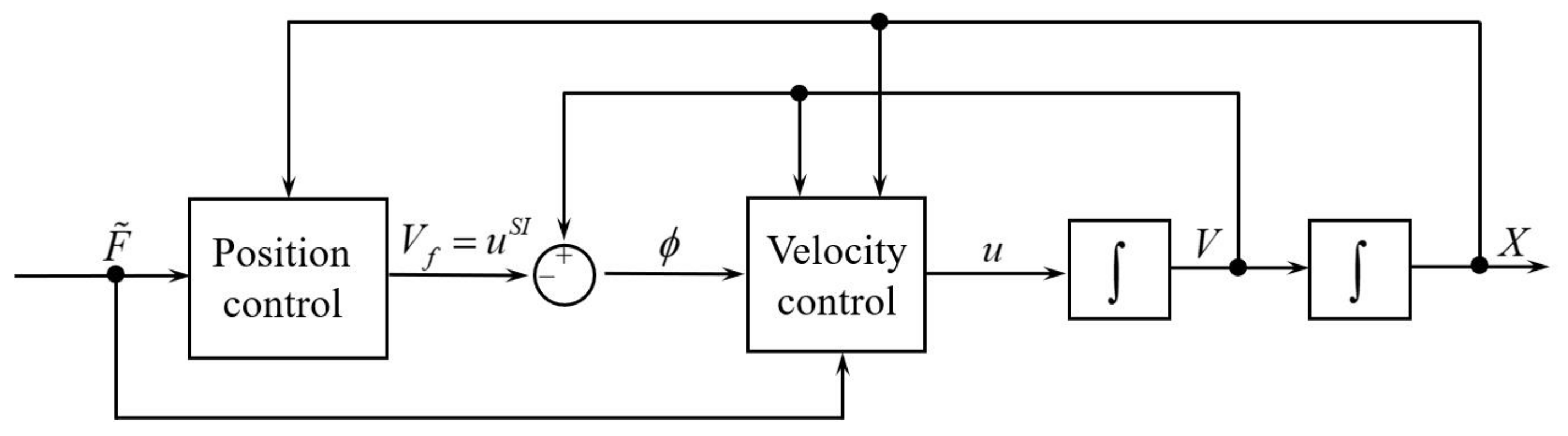
4. Design for Control Inputs

The prerequisite for achieving dynamic formation control is the forming of rigid formation. The control input will be studied next from two perspectives: formation acquisition and dynamic transformation of the formation.
From the previous section, the actual relative position of the two agents is d i j = X i X j , the desired relative position is d ˜ i j = X ˜ i X ˜ j > 0 , and the distance error is
ω i j = d i j d ˜ i j , i , j E ˜
where ω = , ω i j , R l , and d i j = d i j T d i j 1 2 . Since it is desired to achieve a dynamic transformation of the distance between the agents, the desired distance d ˜ i j is a function about t. Substituting (5) into (8) and simplifying the derivative with respect to ω i j , we obtain
ω ˙ i j = d d t d i j T d i j 1 2 d ˜ i j = 1 2 d i j T d i j 1 2 · 2 · d i j T d ˙ i j d ˜ ˙ i j = d i j T d i j 1 2 · d i j T · V i V j d ˜ ˙ i j = d i j T · V i V j ω i j + d ˜ i j d ˜ ˙ i j
Let V i j = V i V j represent the relative velocity between agents. Introduce an error quantity δ i j , where δ = , δ i j , R l , such that
δ i j = d i j 2 d ˜ i j 2
For the second-order MAS, we design the acceleration-level formation acquisition control law as
u = α ϕ + V ˙ f R G T X δ
where
V f 1 = β R G T X δ
Control gains α > 0 , β > 0 are two constants that are sufficiently small. For the dynamic transformation of the formation, V f in (11) is set to
V f = V f 2 = R G + X β δ + D V + V D
The R G + is the pseudo-inverse matrix of R G . D V = , d i j d ˙ i j , . V D is associated with the movement of the formation as a whole and can be expressed as
V D = V t + ϖ X i n V ˙ D = V ˙ t + ϖ ˙ X i n + ϖ V i n
V t and ϖ denote the translational and angular velocities during rigid formation motion, respectively. The Lyapunov functions W connected to the potential and kinetic energies are necessary since the mistakes in the second integrator multi-agent model come from the position and velocity quantities. The system stability can be proven if this error can be shown to be asymptotically stable with time.
W = W 1 + W 2
where W 1 is relevant to the position error and W 2 is relevant to the velocity error, respectively, denoted as
W 1 = 1 4 δ T δ W 2 = 1 2 ϕ T ϕ
Deriving W 1 along time t, we obtain
W ˙ 1 = 1 2 i , j E ˜ δ i j T δ ˙ i j
From (8) and (9), we obtain that
δ i j = d i j 2 d ˜ i j 2 = ω i j + d ˜ i j 2 d ˜ i j 2 = ω i j 2 + 2 ω i j d ˜ i j
Substituting (8) and (18) into (17), we obtain that
W ˙ 1 = 1 2 ( i , j ) E ˜ δ i j T δ ˙ i j = 1 2 ( i , j ) E ˜ ω i j 2 + 2 ω i j d ˜ i j 2 ω i j ω ˙ i j + 2 ω ˙ i j d ˜ i j + 2 ω i j d ˜ ˙ i j = ( i , j ) E ˜ ω i j 2 + 2 ω i j d ˜ i j d i j T · V i V j ω i j + d ˜ i j d ˜ ˙ i j ω i j + d ˜ i j + ω i j d ˜ ˙ i j = ( i , j ) E ˜ ω i j 2 + 2 ω i j d ˜ i j d i j T · V i V j d ˜ i j d ˜ ˙ i j = δ T R G T X · V D V
Since ϕ = V V f , substituting (16) and (19) into (15), we obtain that
W ˙ = W ˙ 1 + W ˙ 2 = δ T R G T X · V f D V + ϕ T u + R G T X ω V ˙ f = β δ T δ ˙ α ϕ T ϕ ˙ 2 m i n β , α W
From (15), (16) and (21), we know that for t , W 0 , W ˙ < 0 . Therefore, it follows from Barbalat’s Lemma that the error quantity is monotonically decreasing, i.e., the whole system tends to stabilize.
Remark 1.
In contrast to the linear model described above, if this control approach is to be extended to the motion of Surface Vessel systems (SVs) and AUVs, it is first necessary to model the nonholonomic kinematics of the vehicle, embed the velocity-level control inputs into the torque and force-level control laws, and then add adaptive control tools to achieve compensation of the unknown parameters. Research on SVs can be found in [27,28].

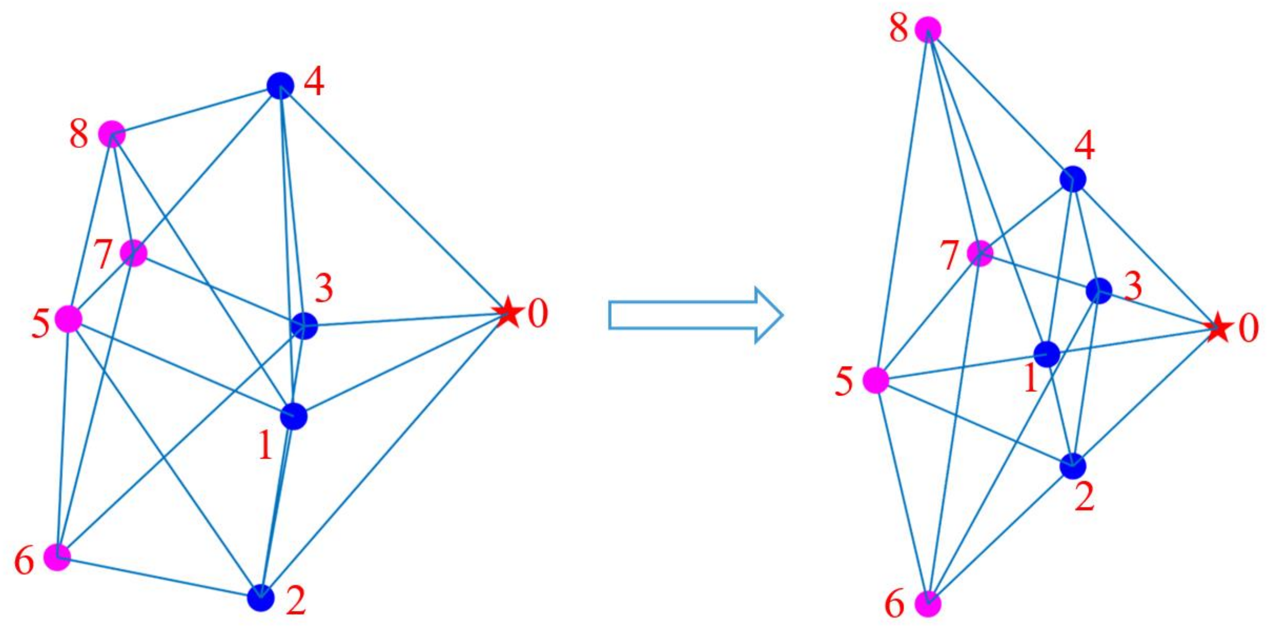
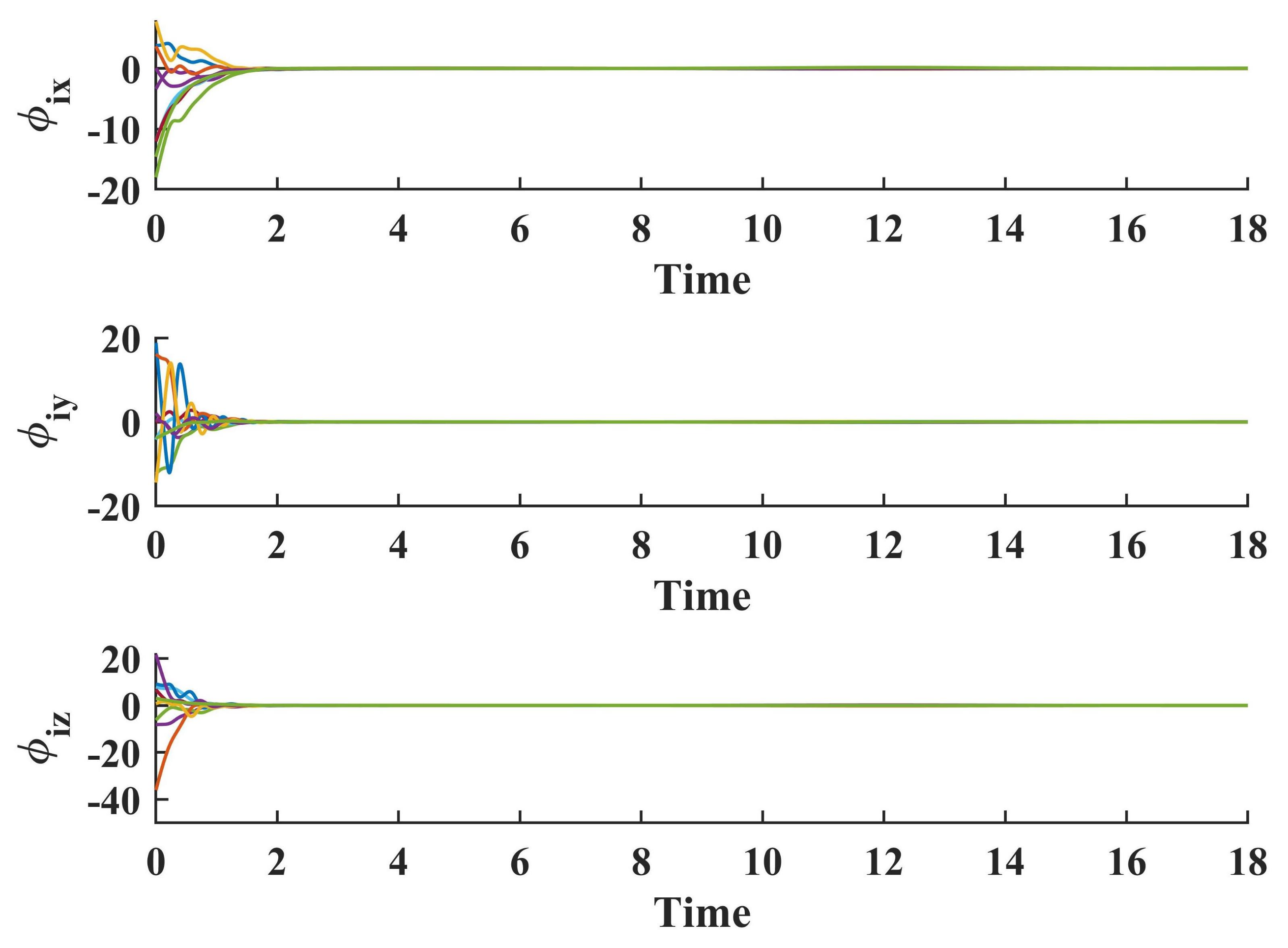
5. Simulation Results

The simulation of formation acquisition and rigid formation dynamic transformation for the aforementioned distance-based formation control rule is obtained in this part using the MATLAB software. Consider an MAS with nine agents n = 9 in 3D space, assuming that the desired formation is a quadrilateral cone, as shown in Figure 3. Let this quadrilateral cone have minimum rigidity to ensure that no flip occurs during the formation operation. The number of edges is required to satisfy l = 3 n 6 = 21 . The leader is located at the vertex of the prism, and the followers are located at other positions.
Assume that the initial positions of the nine agents are set arbitrarily by the operator, and suppose that the initial positions are X 1 = 0.3 , 0.7 , 0.3 , X 2 = 0 , 0.2 , 1 , X 3 = 0.2 , 1.3 , 0 , X 4 = 0 , 0.1 , 1.05 , X 5 = 0.5 , 1.2 , 0.1 , X 6 = 0.7 , 0.2 , 0.8 , X 7 = 0.8 , 0.9 , 0.3 , X 8 = 0.9 , 0.1 , 0.9 , X 0 = 1 , 0 , 0.1 . Assume that the coordinates of the points in the desired formation are X ˜ 1 = 0 , 1 , 0 , X ˜ 2 = 0 , 0 , 1 , X ˜ 3 = 0 , 1 , 0 , X ˜ 4 = 0 , 0 , 1 , X ˜ 5 = 1 , 2 , 0 , X ˜ 6 = 1 , 0 , 2 , X ˜ 7 = 1 , 2 , 0 , X ˜ 8 = 1 , 0 , 2 , X ˜ 0 = 1 , 0 , 0 . According to Figure 3, we obtain V ˜ and E ˜ as
V ˜ = 1 , 2 , , 9
E ˜ = 0 , 1 , 0 , 2 , 0 , 3 , 0 , 4 , 1 , 2 , 2 , 3 , 3 , 4 , 4 , 1 , 1 , 5 , 2 , 6 , 3 , 7 4 , 8 , 5 , 6 , 6 , 7 , 7 , 8 , 8 , 5 , 1 , 6 , 2 , 7 , 3 , 8 , 4 , 5 , 5 , 7 .
The desired distance between agents is d ˜ 01 = d ˜ 02 = d ˜ 03 = d ˜ 04 = d ˜ 15 = d ˜ 26 = d ˜ 37 = d ˜ 48 = d ˜ 12 = d ˜ 23 = d ˜ 34 = d ˜ 42 = 2 , d ˜ 56 = d ˜ 67 = d ˜ 78 = d ˜ 85 = 2 2 , d ˜ 16 = d ˜ 27 = d ˜ 38 = d ˜ 45 = 6 , d ˜ 57 = 2 . Figure 4 presents the process of the desired formation of a second-order MAS from any initial condition, which is necessary for the dynamic transformation of rigid formations.
To perform the dynamic formation of a fixed formation, it is necessary only to modify the distance between agents simultaneously during the operation. Design a function t related to t, making the coordinates of each point change with t, and we finally achieve the dynamic formation.
t = sin 0.4 t + 1
The variation laws of each agent coordinate are as follows:
X ˜ i t = X i 0 t
where X i 0 are the coordinates of each agent of the desired formation in Figure 3. Set the translational V t and angular velocities ϖ of the formation movement as
V t = 5 c o s 0.3 t , 5 s i n 0.3 t , 0
Control gains are assumed to be α = 2 , β = 2 . The MAS achieves the dynamic transformation of rigid formations with the preliminary conditions and control law in (11). The simulation results are shown in Figure 4. Assuming that the multi-agent system rigid formation encounters a narrow alleyway during operation, the expansion and contraction transformation of the formation can ensure safe passage while maintaining the shape of the quadrilateral cone formation (the control target is the acceleration of the leader, and the follower always keeps a specific distance and orientation from the leader under the action of the rigid formation), and this example verifies the effectiveness of the control law. The trajectory of the navigator is marked with a red dashed line. Two gray-green rectangles are used to simulate narrow alleyways.
From Figure 5, the distance error between neighboring agents gradually tends to zero, indicating that the multi-agent formation can move from any initial position to the preset desired position.
Figure 6 presents the error between the actual velocity and the desired velocity of each agent in x, y and z directions, and it is evident that, after a certain range of fluctuations, the error gradually becomes zero. Figure 7 shows the components of the control input u in the x, y, and z directions of the acceleration level. Figure 8 shows the variation of the control inputs of the nine agents. From the above figures, we can see that the system can complete the formation acquisition in 2 s, providing the dynamic scaling of rigid formations.

6. Conclusions

This paper proposes a rigid matrix-based method to achieve the dynamic formation control of MAS in three-dimensional space. A distributed formation control law about the second-order integrator model is designed. This control law includes two parts, formation formation and formation movement, and each agent can form a preset formation from any initial condition within 2 s, after which the distance-based control method is used to set the expected distance between agents as a time-dependent function to realize the dynamic transformation of MAS formation. Collisions outside the formation are avoided while ensuring that no collisions occur inside the formation. Future research priorities are listed here, for example, applying the control approach proposed in this paper for mass points to objects with motion constraints.

Author Contributions

Conceptualization, G.T.; methodology, C.Y.; software, L.L.; validation, Y.C.; formal analysis, K.H.; investigation, G.T. and L.L.; resources, L.L. and D.L.; data curation, L.L.; writing—original draft preparation, G.T.; writing—review and editing, L.L. and D.L.; visualization, C.Y.; supervision, D.L. and C.X.; project administration, D.L. and C.X.; funding acquisition, D.L. and C.X. All authors have read and agreed to the published version of the manuscript.

Funding

This research was funded by the National Natural Science Foundation of China, Grant 62001428; the Key R&D Program of Shanxi Province, Grant 202102020101010; the Research Project Supported by the Shanxi Scholarship Council of China, Grant 2022-144, and the Scientific and Technological Innovation Programs of Higher Education Institutions in Shanxi, Grant 2020L0309.

Data Availability Statement

Not applicable.

Conflicts of Interest

The authors declare no conflict of interest.

References

  1. Animasaun, I.L.; Shah, N.A.; Wakif, A.; Mahanthesh, B.; Sivaraj, R.; Koriko, O.K. Conceptual and Empirical Reviews I. In Ratio of Momentum Diffusivity to Thermal Diffusivity: Introduction, Meta-Analysis, and Scrutinization; Chapman and Hall/CRC: New York, NY, USA, 2022. [Google Scholar]
  2. Wen, G.; Zheng, W.X. On Constructing Multiple Lyapunov Functions for Tracking Control of Multiple Agents with Switching Topologies. IEEE Trans. Automat. Control 2019, 64, 3796–3803. [Google Scholar] [CrossRef]
  3. Yongzhao, H.; Xiwang, D.; Qingdong, L.; Zhang, R. Distributed Fault-Tolerant Time-Varying Formation Control for Second-Order Multi-Agent Systems with Actuator Failures and Directed Topologies. IEEE Trans. Circuits Syst. II Express Briefs 2017, 65, 774–778. [Google Scholar]
  4. Meng, Z.; Anderson, B.; Hirche, S. Formation control with mismatched compasses. Automatica 2016, 69, 232–241. [Google Scholar] [CrossRef]
  5. Deng, J.; Wang, L.; Liu, Z. Attitude synchronization and rigid formation of multiple rigid bodies over proximity networks. Automatica 2018, 125, 109388. [Google Scholar]
  6. Olfatisaber, R.; Murray, R.M. Graph rigidity and distributed formation stabilization of multi-vehicle systems. In Proceedings of the 41st IEEE Conference on Decision and Control, Las Vegas, NV, USA, 10–13 December 2002. [Google Scholar]
  7. Krick, L.; Broucke, M.E.; Francis, B.A. Stabilization of infinitesimally rigid formations of multi-robot networks. Int. J. Control 2009, 82, 423–439. [Google Scholar] [CrossRef]
  8. Oh, K.K.; Ahn, H.S. Formation control of mobile agents based on inter-agent distance dynamics. Automatica 2011, 47, 2306–2312. [Google Scholar] [CrossRef]
  9. Cai, X.; de Queiroz, M. Multi-agent formation maneuvering and target interception with double-integrator model. In Proceedings of the American Control Conference, Portland, OR, USA, 4–6 June 2014. [Google Scholar]
  10. Cai, X.; de Queiroz, M. Multi-agent formation maintenance and target tracking. In Proceedings of the American Control Conference (ACC), Washington, DC, USA, 17–19 June 2013. [Google Scholar]
  11. Zhang, P.; Queiroz, M.D.; Cai, X. Three-Dimensional Dynamic Formation Control of Multi-Agent Systems Using Rigid Graphs. J. Dyn. Syst. Meas. Control 2015, 137, 111006. [Google Scholar] [CrossRef]
  12. Deghat, M.; Anderson, B.; Lin, Z. Combined Flocking and Distance-Based Shape Control of Multi-Agent Formations. IEEE Trans. Automat. Control 2016, 61, 1824–1837. [Google Scholar] [CrossRef]
  13. Cai, X.; Queiroz, M.D. Rigidity-Based Stabilization of Multi-Agent Formations. J. Dyn. Syst. Meas. Control 2013, 136, 014502. [Google Scholar] [CrossRef]
  14. Oh, K.K.; Ahn, H.S. Distance-based undirected formations of single-integrator and double-integrator modeled agents in n-dimensional space. Int. J. Robust Nonlinear Control 2013, 24, 1809–1820. [Google Scholar] [CrossRef]
  15. Cao, M.; Morse, A.S.; Yu, C.; Anderson, B.; Dasgupta, S. Maintaining a Directed, Triangular Formation of Mobile Autonomous Agents. Commun. Inf. Syst. 2011, 11, 1–16. [Google Scholar]
  16. Park, M.C.; Anderson, B.; Sun, Z.; Ahn, H.S. Stability analysis on four agent tetrahedral formations. In Proceedings of the 53rd IEEE Conference on Decision and Control, Los Angeles, CA, USA, 15–17 December 2015; pp. 631–636. [Google Scholar]
  17. Sun, Z.; Mou, S.; Anderson, B.; Morse, A.S. Non-robustness of gradient control for 3-D undirected formations with distance mismatch. In Proceedings of the Australian Control Conference, Fremantle, WA, Australia, 4–5 November 2013. [Google Scholar]
  18. Babazadeh, R.; Selmic, R. Distance-Based Multiagent Formation Control with Energy Constraints Using SDRE. IEEE Trans. Aerosp. Electron. Syst. 2019, 56, 41–56. [Google Scholar] [CrossRef]
  19. Queiroz, M.D.; Cai, X. Formation Maneuvering and Target Interception for Multi-Agent Systems via Rigid Graphs. Asian J. Control 2015, 17, 1174–1186. [Google Scholar]
  20. Khaledyan, M.; Liu, T.; Queiroz, M.D. Flocking and Target Interception Control for Formations of Nonholonomic Kinematic Agents. IEEE Trans. Control Syst. Technol. 2019, 28, 1603–1610. [Google Scholar] [CrossRef] [Green Version]
  21. Cao, M.; Morse, A.S.; Yu, C.; Anderson, B.D.O.; Dasguvta, S. Maintaining a Directed, Triangular Formation of Mobile Autonomous Agents. In Proceedings of the 46th IEEE Conference on Decision and Control, New Orleans, LA, USA, 12–14 December 2007; pp. 3603–3608. [Google Scholar]
  22. Dorfler, F.; Francis, B. Geometric Analysis of the Formation Problem for Autonomous Robots. IEEE Trans. Automat. Control 2010, 55, 2379–2384. [Google Scholar] [CrossRef]
  23. Olfati-Saber, R.; Murray, R.M. Distributed cooperative control of multiple vehicle formations using structural potential functions. IFAC Proc. Vol. 2002, 35, 495–500. [Google Scholar] [CrossRef]
  24. Sun, Z.; Park, M.-C.; Anderson, B.D.O.; Ahn, H.-S. Distributed stabilization control of rigid formations with prescribed orientation. Automatica 2017, 78, 250–257. [Google Scholar] [CrossRef]
  25. Anderson, B.; Yu, C.; Fidan, B.; Hendrickx, J. Rigid graph control architectures for autonomous formations. Control Syst. IEEE 2008, 28, 48–63. [Google Scholar]
  26. Asimow, L.; Roth, B. The rigidity of graphs, II. J. Math. Anal. Appl. 1979, 68, 171–190. [Google Scholar] [CrossRef]
  27. Vu, V.T.; Tran, Q.H.; Pham, T.L.; Dao, P.N. Online Actor-critic Reinforcement Learning Control for Uncertain Surface Vessel Systems with External Disturbances. Int. J. Control Autom. 2022, 20, 1029–1040. [Google Scholar] [CrossRef]
  28. Vu, V.T.; Pham, T.L.; Dao, P.N. Disturbance observer-based adaptive reinforcement learning for perturbed uncertain surface vessels. ISA Trans. 2022, in press. [Google Scholar] [CrossRef]
Figure 1. (a) Flexible frame. (b) Minimum rigidity graph. (c) Rigidity graph.
Processes 10 01961 g001
Figure 2. Second-order integrator control model.
Processes 10 01961 g002
Figure 3. Desired formation.
Processes 10 01961 g003
Figure 4. Formation acquisition.
Processes 10 01961 g004
Figure 5. Dynamic formation trajectory diagram.
Processes 10 01961 g005
Figure 6. Distance errors between agents i and j.
Processes 10 01961 g006
Figure 7. Velocity errors in x, y, and z directions.
Processes 10 01961 g007
Figure 8. Control inputs for dynamic formation.
Processes 10 01961 g008
Publisher’s Note: MDPI stays neutral with regard to jurisdictional claims in published maps and institutional affiliations.

