Two-Step Optimal-Setting Control for Reagent Addition in Froth Flotation Based on Belief Rule Base

Abstract

Reagent addition is an important operation in the froth flotation process. In most plants, it is manually regulated according to the operator’s experience, by observing the surface features of the froth. Due to the drawbacks of manual operation, large fluctuations in the process are common, resulting in unexpected process indexes. Thus, we investigated the relationship between reagent addition, feed conditions (including ore properties, slurry density, and slurry flow rate), and froth image features based on the mechanism of froth flotation and production technology of gold-antimony flotation. Then, we proposed a two-step optimal-setting control strategy for reagent addition, which included a basic dosage pre-setting model and a feedback reagent addition compensation model. According to operating conditions and ore properties, the pre-setting model was developed using a belief rule base (BRB) method based on an evidential reasoning approach (RIMER), which could effectively address the uncertainties of operator experience and historical data. The model parameters of the BRB were then optimized using a state transition algorithm (STA). In terms of the offsets of the froth image features, the feedback compensation model using rule-based reasoning (RBR) was built. Simulation results using a STA-optimized BRB, GA-optimized BRB, least squares support vector machine (LSSVM), and artificial neural network (ANN) were compared. Finally, industrial test results confirmed that the reagent addition system based on the proposed method could satisfy the requirements for automatic reagent addition in an industrial production environment. This is of great significance for improving the production efficiency of flotation plants.

1. Introduction

Froth flotation is widely used for separating valuable minerals from gangue. The essential mechanism of froth flotation is that reagents are added into the slurry to regulate the physicochemical properties of the particles [1]. To obtain a high concentrate grade and high recovery of the target metals, the optimal control of the types and quantities of reagents is important in the flotation process [2]. Due to the complex mechanisms involved and the long production process, there is an intricate relationship between the flotation performance and process variables, with strong coupling and significant uncertainties. Accordingly, in view of the difficulty of the online measurement of key process parameters, reagent addition control is performed by operators, based on their observation of the surface features of the froths, in almost all plants in China. The processes are usually regulated at very low frequency during the night and different operators have different levels of experience, which often results in a fluctuation in performance. Moreover, optimal operation of the process cannot be achieved, even when managed by very experienced operators [3]. Thus, the automatic and optimal control of reagent addition in the froth flotation processes has been an area of active research for many years.

Experiments and statistical methods are commonly used to determine optimal reagent addition. For example, Rath et al. [4] developed a quadratic response model using experimental data to determine the relationship between flotation reagents and both the Fe grade and recovery in a hematite flotation process. In studies by Azizi et al. [5] and Vieceli et al. [6], prediction models of process indexes were built based on experimental findings to identify the optimum reagent dosage.

Objective-based optimization methods are effective for optimal control in industrial processes if effective process models can be established [7,8,9]. However, for industrial flotation processes, it is very difficult to obtain a proper mathematical model.

The surface features of froths are important parameters that define the state of the process. They have been used for control and optimization of the froth flotation process in an increasing number of studies [10,11,12,13,14,15,16]. Meanwhile, in practice, operational experience is very important for reagent addition and has been the topic of some investigations. For example, Jahedsaravani et al. [10] modeled a high correlation between froth features (bubble size and velocity) and several process variables (pH, air-flow rate, and frother dosage) using neural networks. Zhang et al. [11] introduced a nonlinear model based on the wavelet-based Hammerstein–Wiener method to build a causal relationship between reagent dosage and bubble size distribution. Zhu et al. [12] presented a model predictive control method to calculate the reagent dosage by tracking a target probability density function (PDF) of bubble size. Zhang and Gao [13] designed a digital twin system for iron reverse flotation reagent addition. Based on the froth images and transformer algorithm, the flotation dosing model automatically updates the reagent system.

Kaartinen et al. [14] developed a reagent dosage control system based on expert rules in terms of empirical knowledge between image variables (froth color, bubble size distribution, froth speed, bubble collapse rate, and bubble load) and reagent dosage in zinc flotation. Xie et al. [15] proposed a sensitive froth image feature-based reagent addition control strategy based on the interval type II fuzzy control method. However, in most of these studies, only feed grade and froth features were taken as inputs. They did not consider the change in other working conditions that could have a significant impact on flotation performance, such as slurry density and slurry flow rate. The complexity of the process causes many uncertainties; it is impossible to build correlations between the process outputs and the inputs, states, and operating parameters.

Therefore, to develop an automatic control method which can fuse all the significant variables in the process and effectively eliminate the uncertainties involved, we propose an optimal-setting control strategy for reagent addition that considers both the feed conditions and froth image features for gold-antimony flotation. This strategy adopts a belief rule base (BRB) method, which has been demonstrated to be more suitable for uncertain information [17,18,19], to address the optimal-setting problem and identify optimal froth features to control the process better.

The rest of this study is arranged as follows: Section 2 presents the flotation process and an analysis of the relationship between all the variables. Based on this analysis, a two-step optimal-setting control strategy for reagent addition is developed in Section 3. The effectiveness of the strategy is confirmed through simulation and industrial testing in Section 4, and Section 5 summarizes the main conclusions.

2. Process Description and Analysis of Reagent Addition

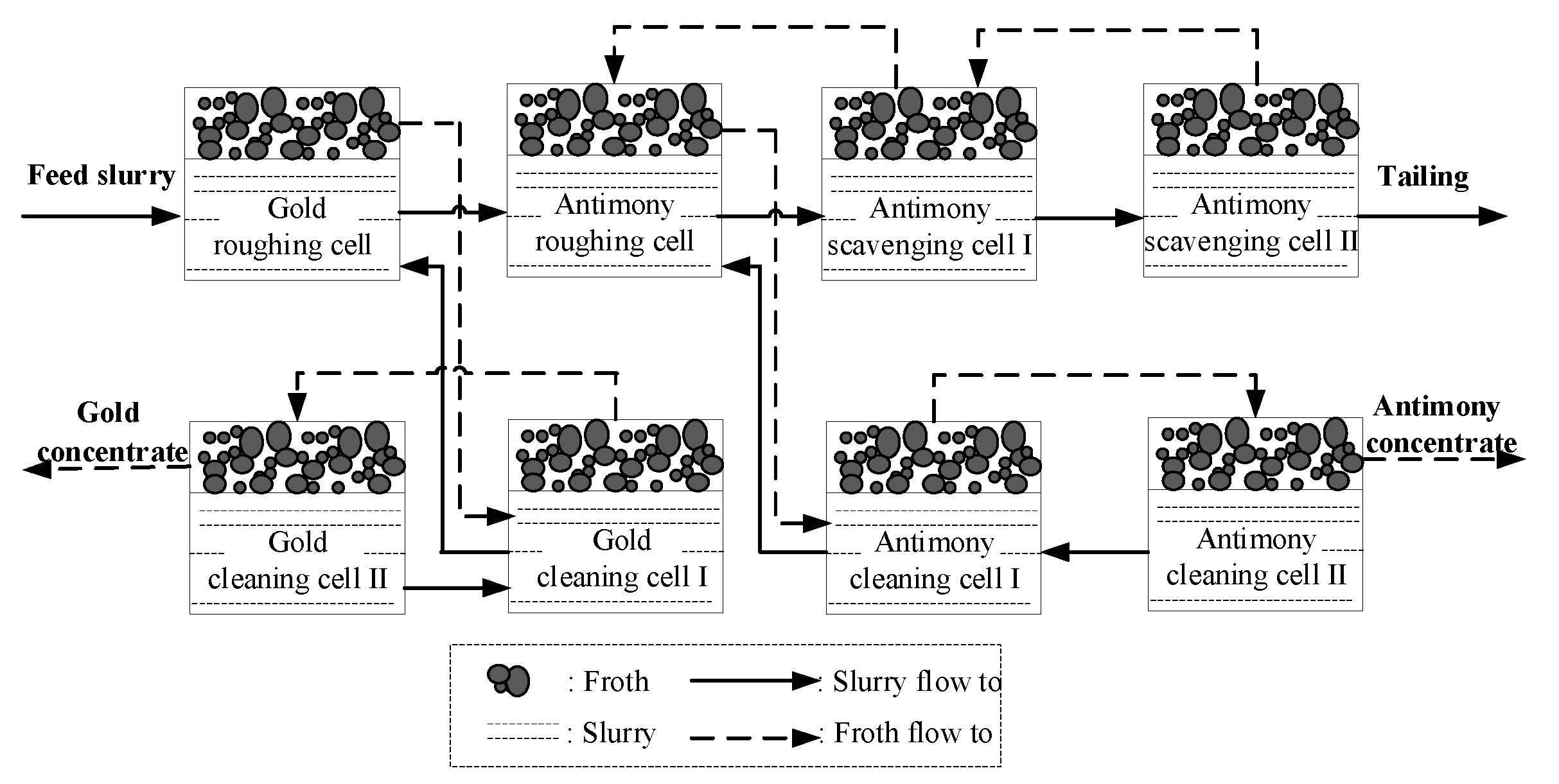
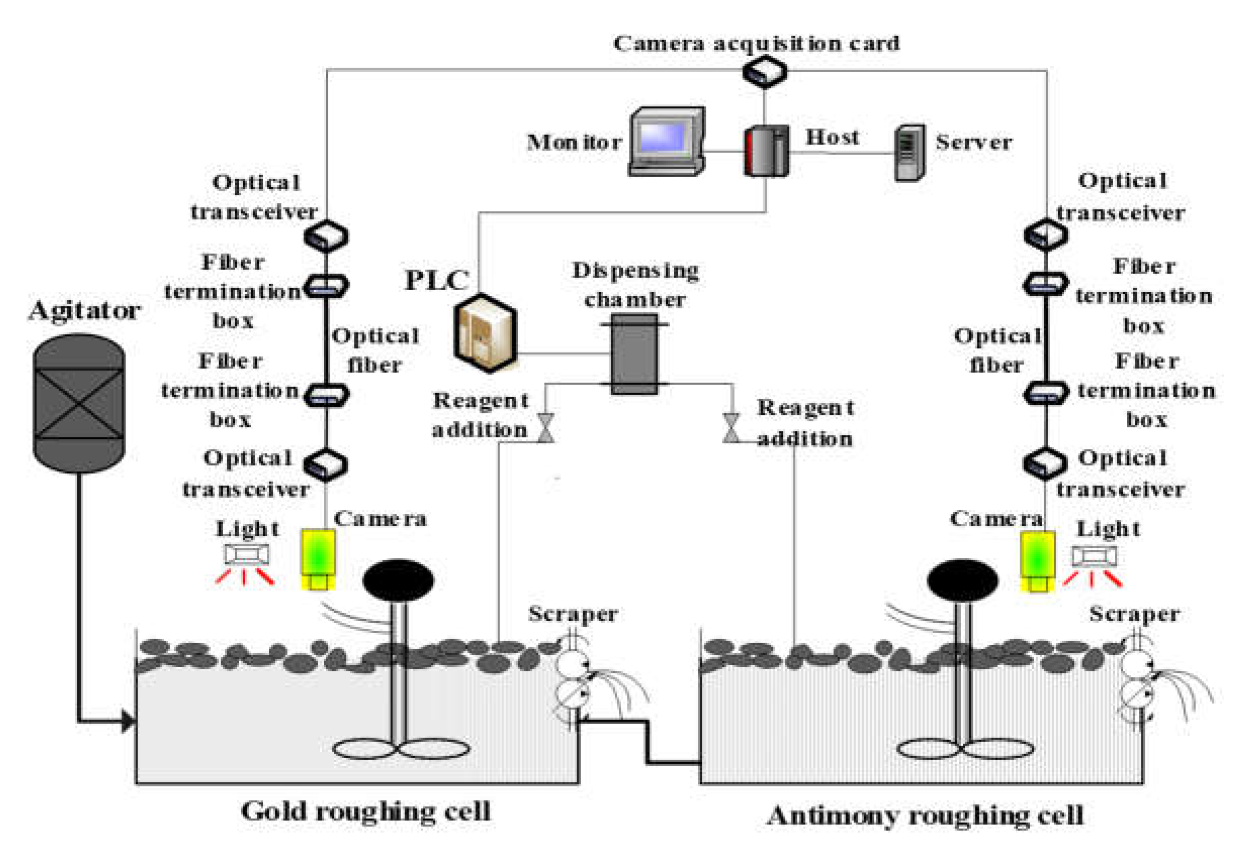
2.1. Process Description

The gold-antimony froth flotation in this study adopts a part priority-mixed flotation process, meaning gold flotation is performed in alkaline pulp, followed by antimony flotation in acidic pulp. The process diagram is shown in Figure 1.

In this process, the feed flow rate and slurry level are measured online and can be regulated through a distributed control system (DCS). The particle size in the feed slurry is manually measured off-line every two hours, and feed ore grades (sampled before milling) and technical indices (tailing grade and concentrate) are measured off-line every eight hours, which causes control delay. Froth depth, measured by a floating level meter, is set to be a specific value and automatically controlled by regulating the slurry level. Therefore, the status of the froths is the most important state in the froth flotation process. Reagent addition is mainly manually controlled according to feed conditions and the status of the froths.

Due to the complex physicochemical reactions in the gold-antimony flotation process, there are strong nonlinearities and significant uncertainties between feed conditions, reagent addition, and flotation performance. Thus, it is necessary to implement automatic and optimal control of reagent addition to stabilize the process and reduce labor intensity. This can increase efficiency and improve the economic benefits of mineral processing.

2.2. Reagent Addition Analysis

The relationships between reagent addition, feed conditions, and froth image features are very complex [14]. Their analysis is described in the following section.

Feed conditions refer to the ore properties, slurry flow rate, and slurry density.

2.2.1. Ore Properties

In mineral engineering, ore properties, including ore floatability, compositions, grade, mineral dissemination characteristics, ore paragenesis, and existent morphology, are the critical factors used to determine how the froth flotation process should be operated. For ores with certain properties, there is an optimal amount of reagent that yields the best performance [20]. Considering that many factors cannot be measured online and are very difficult and expensive to be measured offline, only the ore compositions (grade) were measured in daily production to characterize ore properties.

2.2.2. Slurry Flow Rate and Slurry Density

When slurry flow rate (in t/h) increases, reagent addition needs to be correspondingly increased to maintain the qualified production index.

The slurry density (C) refers to the solid mass fraction of the slurry. A high slurry density requires a long flotation time and improves recovery but may reduce the grade of the concentrate. Meanwhile, within a certain range, the higher the slurry density, the higher the concentration of the reagent in the slurry, and the reagent dosage added per ton of ore can be reduced [21].

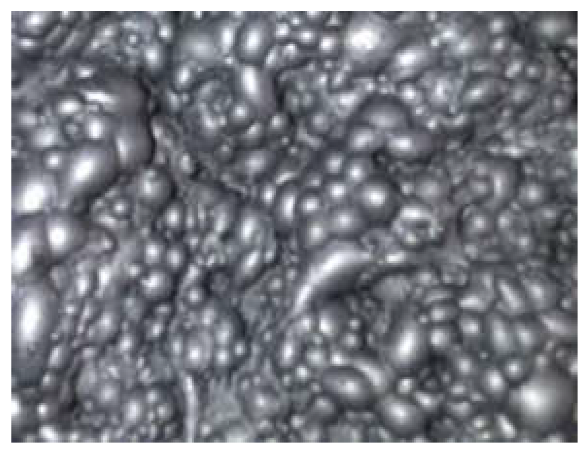
2.2.3. Froth Features

The surface features of froths have been used by many researchers as the main state variables for reagent addition control and optimization [14]. When the characteristics of the ore are stable, changes of the froth features indicate how reagents need to be regulated. In the actual production process, an adjustment in any reagent can cause a change of many froth image features [13]. The relationships between the froth features and reagents are too complex and uncertain and can only be described in vague terms such as the change of direction and degree.

Additionally, from long-term observation of the gold-antimony flotation process, we know that, under different ore grades, the froth status is clearly different.

2.3. Challenges and Difficulties in Reagent Addition

From the above analysis, it is evident that the following challenges exist in the reagent addition setting control:

• Uncertainties in the process, including uncertainties caused by immeasurable ore properties, complicated and unclear mechanisms [15], intricate relationships and unknown correlations between the variables, and large measurement errors contained in the data. These introduce a large amount of uncertainty to reagent addition.
• The frequent changing of ore properties is a significant issue, which causes difficulty in many flotation plants because good ore resources are eventually exhausted [16,20]. As in many other flotation processes, when the feed grade does not significantly change in gold-antimony flotation, working conditions are relatively stable and the flotation process is easy to control. On the contrary, the difficulty of reagent addition control increases.
• The pH value and process indices are key feedback control measures. However, they cannot be measured online or even at a very low frequency. Therefore, froth features are mainly used as feedback and operator experience becomes more important.

Accordingly, based on the difficulties presented by the froth flotation mechanism and real production practices, a two-step optimal-setting control strategy for reagent addition is investigated, which considers the aforementioned parameters and addresses the uncertainties in operator experience and process data.

3. Optimal-Setting Control for Reagent Addition

The two-step optimal-setting strategy contains a pre-setting step using BRB-based RIMER methods according to feed conditions, and a feedback-setting step using IF-THEN rules and RBR according to froth features. The details of the strategy are described in the next section.

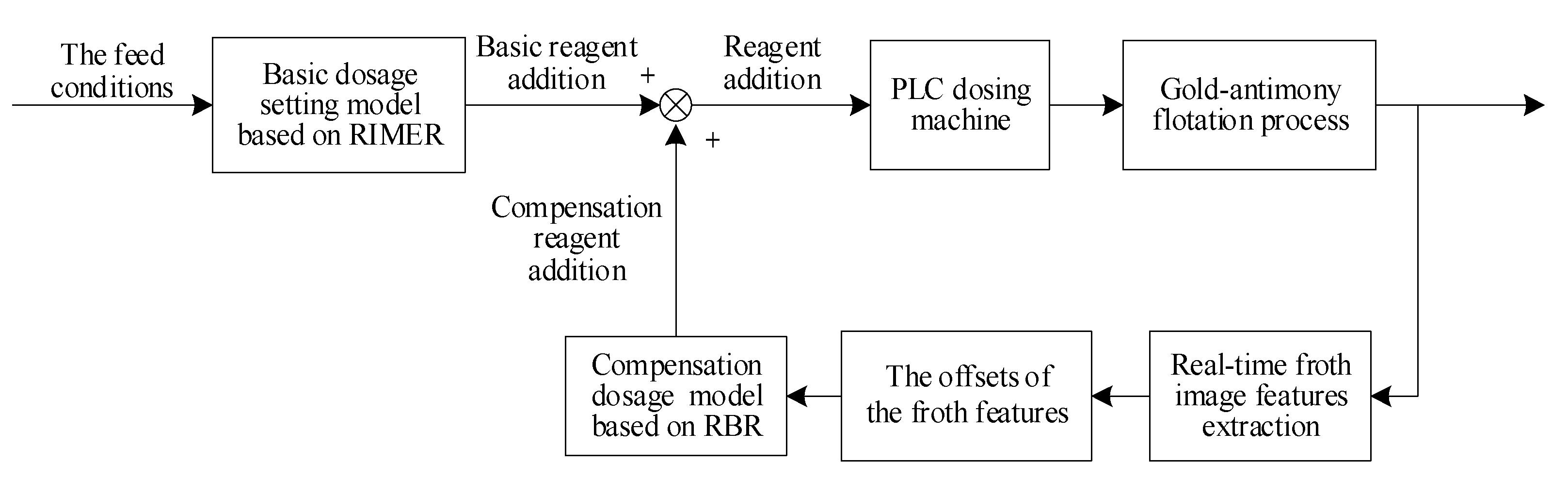
3.1. Optimal-Setting Control Strategy of Reagent Addition

In froth flotation, feed conditions are the main factors that determine the amount of reagent required. Therefore, a basic amount of reagent is accordingly preset. The surface features of the froths are state variables that provide feedback information and indicate whether regulation is needed for the reagents. The two-step optimal-setting control strategy of reagent addition based on feed conditions and froth features is shown in Figure 2.

As shown in Figure 2, the optimal-setting control strategy includes a basic dosage pre-setting model using RIMER, and a feedback reagent addition compensation model based on RBR. Then, the sum of the basic reagent addition and compensate reagent addition is taken as the optimal reagent addition and transferred to the dosing machine controlled by the PLC for execution.

3.2. Reagent Addition Pre-Setting Based on RIMER

Considering the uncertainties listed in Section 2.3., we required a method that could effectively address uncertainty.

Yang et al. [17] proposed RIMER; it adds antecedent attribute weights, rule weights, and belief degrees of results, which expand the scope of rule description while also fully combining randomness and fuzziness of knowledge. This meets the requirements for the practical application of reagent addition control knowledge. The rule base, which consists of a series of belief rules, is called the BRB.

Based on the BRB, the inference of knowledge is performed via an evidential reasoning (ER) approach. Meanwhile, parameter optimization can be implemented using an optimization algorithm.

3.2.1. BRB Structure and Representation for Basic Reagent Addition Pre-Setting

In this study, we constructed five BRBs for reagent addition in gold rougher flotation and antimony rougher flotation, respectively. The BRB structure for the tth reagent is,

$$\begin{array}{l}{R}_k^{\prime }:if{X}_{1}is{A}_1^{k}and{X}_{2}is{A}_2^{k}and\cdots and{X}_{M}is{A}_{M_k}^{k}then\\ O_t:\left\{\left(D_{t1},{\beta }_{t1,k}\right),\left(D_{t2},{\beta }_{t2,k}\right),\cdots \left(D_{tN},{\beta }_{tN,k}\right)\right\}with{\theta }_{tk}and{\delta }_{t1,k},...,{\delta }_{t{M}_k,k}\end{array}$$

(1)

where, t = 1, …, T, T is the number of the reagents, $O_t$ is the tth reagent in the output attributes, and N is the number of output levels. X = ($X_1,X_2,\cdots ,X_{M_k}$) refers to the antecedent attributes in the kth rule. M_k is the number of the antecedent attribute in the kth rule. $X_i$∈U. U = {$U_i$, i = 1, ..., M} is the antecedent attributes set. M is the total number of the antecedent attributes. Therefore, M_k ≤ M. N is the number of output levels. k = 1, …, L, denotes the kth rule. $A_i^k$ (i = 1, …, M_k, k = 1, …, L) is the referential value of the ith antecedent attribute $U_i$ in the kth rule. $A_i^k$∈A_i. A_i= {A_ij, j = 1,..., J_i} is a set of referential values for the ith antecedent attribute, and J_i is the number of referential values of the ith antecedent attribute. ${\beta }_{j,k}$ (j = 1, …, N) is the belief degree of the output result, $D_j$, in the kth rule. Term ${\theta }_k$ is the rule weight of the kth rule. Attribute weight ${\delta }_{i,k}$ refers to the importance degree of $U_i$, compared with other antecedent attributes in the kth rule. Without loss of generality, suppose ${\delta }_i={\delta }_{i,k}$ in the BRB. For different reagents, it can have different output levels.

For gold flotation, the antecedent attributes are feed grade, slurry flow rate, and slurry density, which are denoted by $U_1$, $U_2$, and $U_3$, respectively. The consequent attributes are xanthate, CuSO₄, Na₂S, Na₂CO₃, and terpenic oil. For antimony flotation, the antecedent attributes are feed grade, slurry flow rate, and slurry density, and the consequent attributes are xanthate, aerofloat, CuSO₄, Pb (NO₃)₂, and terpenic oil. The referential points need to be selected and quantified before building a specific BRB. The number of referential points should neither be too large nor too small. The referential values should approximately cover the value range of the corresponding attribute. By combining the process data with operator experience, the number of referential points were determined, as shown in

Table 1. Input referential values of antecedent attributes in gold flotation.

Antecedent Attributes	PS	PM	PL
Feed grade (%)	2.05	2.29	2.47
Slurry flow rate (t/h)	10	12	14
Slurry density (%)	25	31	37

,

Table 2. Output referential values of consequent attributes in gold flotation (mL/min).

Consequent Attributes	PS	PM	PL
Xanthate	570	590	620
CuSO4	400	415	430
Na2S	1020	1092	1200
Na2CO3	900	1015	1250
Terpenic oil	8	13	18

,

Table 3. Input referential values of antecedent attributes in antimony flotation.

Antecedent Attributes	PVS	PS	PM	PL	PVL
Feed grade (%)	1	1.41	1.73	2.11	2.76
Slurry flow rate(t/h)	-	10	12	14	-
Slurry density (%)	-	25	31	37	-

and

Table 4. Output referential values of consequent attributes in antimony flotation (mL/min).

Consequent Attributes	PVS	PS	PM	PL	PVL
Xanthate	150	180	210	250	300
Aerofloat	60	90	130	170	200
CuSO4	50	57	65	72	80
Pb (NO3)2	300	330	370	410	440
Terpenic oil	6	23	40	59	88

, where PVS, PS, PM, PL, and PVL denote positive very small, positive small, positive medium, positive large, and positive very large, respectively.

According to the flotation mechanism and operator experience, the initial BRBs of basic reagent addition pre-setting for gold and antimony rougher flotation were built, respectively. For gold flotation, because feed grade, slurry flow rate, and slurry density were all divided into three terms, there were 27 combinations of the three antecedents, leading to 27 rules in total in the rule base. For antimony flotation, because feed grade was divided into five terms and both slurry flow rate and slurry density were divided into three terms, there were 45 combinations of the three antecedents, leading to 45 rules in total in the rule base. All the rules were summarized according to the process knowledge and experience of the operator and metallurgist.

3.2.2. Belief Rule Inference Using the ER Approach

An ER algorithm was developed based on the DS theory [18,19]. In recent years, the ER approach has been applied to engineering design, user satisfaction assessment, product life assessment, trauma outcome prediction, and risk assessment [19]. However, the requirement of real-time in this study was more important than it was in these other test cases. In our study, using an ER approach included the following four steps [17]:

Step 1

Calculate the individual matching degree.

Step 2

Calculate the activation weights.

Step 3

Synthesize the activated rules.

Step 4

Calculate the expected output.

The results inferred from RIMER are the combination of a series of rules, which can produce a continuous output space to achieve fine control of reagent addition.

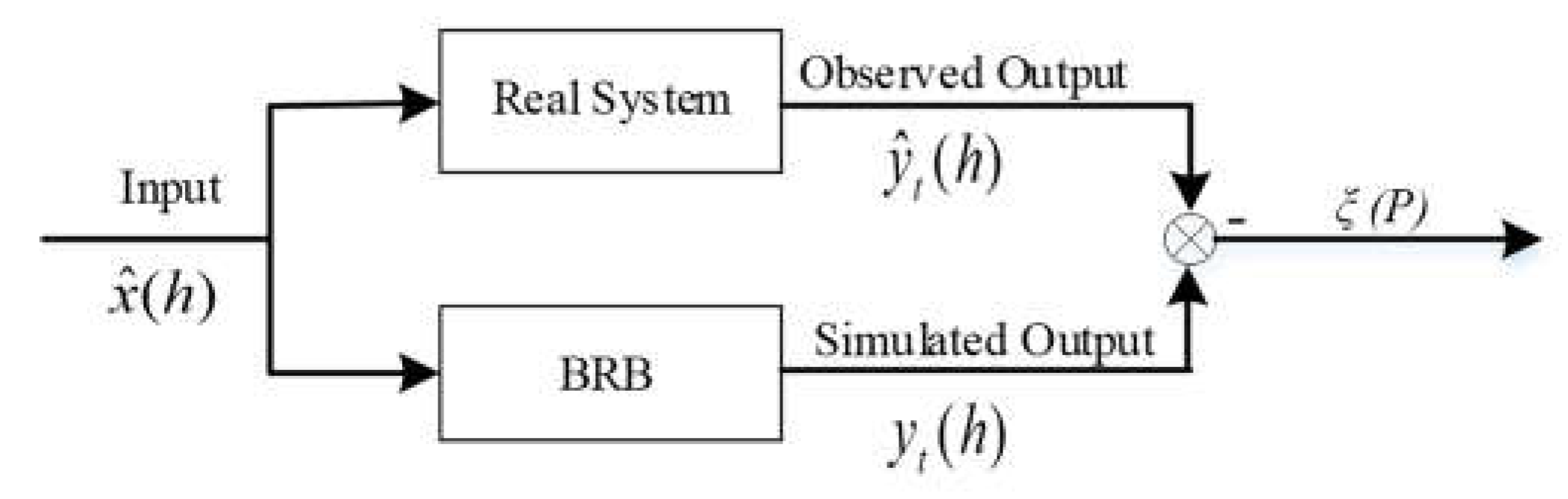
3.2.3. BRB Parameter Optimization

In the inferencing process of the BRB, parameter values, including ${\theta }_{tk}$, ${\delta }_{ti}$, ${\beta }_{tn,k}$, $A_{ij}$, $D_{tn}$, were initially provided by operators based on individual experience of and personal judgment, which are prone to error. Inference performance can be improved if the above parameters are adjusted by autonomous learning. The framework of the optimal learning model used in the BRB expert system is shown in Figure 3, which is referred to in [22].

The objective of our optimal learning model was to minimize the mean absolute error (MAE) between the BRB-based outputs and real reagent addition that was set by the operators, and was defined as follows:

$$\min \left(\xi \left(P\right)\right)=\min \left(\frac{1}{H}{\displaystyle \sum _{h=1}^H\left|y_t\left(h\right)-{\widehat{y}}_t\left(h\right)\right|}\right)$$

(2)

where P is the row vector of the training parameters, $\xi \left(P\right)$ is the objective function, and H is the number of training data. For the hth input $\widehat{x}(h)$ (h = 1, 2, …, H), ${\widehat{y}}_t\left(h\right)$ is the real reagent addition of the tth reagent $O_t$ and $y_t\left(h\right)$ is the BRB-based output of the tth reagent.

Equation (2) is a multi-variable constrained non-linear optimization problem and thus, not easily solved. To solve this complex problem, we used a parameter optimization method based on a state transition algorithm (STA) with demonstrated superior global searching capabilities, convergence properties, and a higher solution precision than some other popular algorithms.

Taking advantage of the two-stage STA, an optimized BRB can be obtained. Using the optimized parameters for inference, the optimized BRB-based output is closer to that of the real reagent addition set by the operators than the output of the initial rules.

3.3. Feedback Compensation Model of Reagent Addition Based Froth Features

By combining information about the process mechanism from operator experience and process data analysis, we selected froth image features that could adequately define the optimal-setting control of reagent addition. The froth features selected for reagent control included gray level, hue, size average, and size variance. These features were extracted by using machine vision technology, which can be found in reference [23].

Probability statistical distributions and optimal intervals of the froth image features were obtained through statistical analysis of the froth features and their corresponding process indices (including recovery and concentrate grade), as shown in Figure 4 and

Table 5. Optimal intervals of froth image features.

Gray Level	Hue	Froth Variance	Froth Size
[86, 128]	[100, 215]	[760, 2180]	[440, 1400]

. At this optimal interval, there was greater than a 90% probability for the indices to be of higher or highest grade. An image of the froth at optimal intervals is shown in Figure 5.

The control objective was to regulate reagents to achieve optimal intervals of froth features. When froth image features were not in the optimal intervals, there needed to be compensation of basic reagent addition. The difference between real-time froth features and the optimal froth feature here is called offset. The mid-value of the optimal interval of a froth feature is regarded as the optimal froth feature. Considering antimony rougher flotation, for instance, the relationship between a single froth image feature and the reagents can be obtained, as shown in

Table 6. The relationship between a single froth feature with each reagent.

Regulating Direction	Aerofloat	Pb (NO3)2	Xanthate	Terpenic Oil	CuSO4
Gray level	Inverse	Direct	Direct	Inverse	Direct
Hue	Direct	No impact	No impact	Inverse	Direct
Size average	Inverse	Direct	Direct	Inverse	Direct
Size variance	Inverse	Direct	Direct	Inverse	Direct

. In Table 6, the terms inverse and direct mean that there is an inverse ratio and direct proportional relationship between the froth feature and the reagent, respectively. No impact means that the froth feature did not change with the amount of reagent.

Accordingly, a reagent addition compensation model can be built based on these froth features. In this model, knowledge is presented as IF-THEN rules, and BRB is adopted. The offset of the gray level is defined as,

$$\Delta gra{y}_i=gra{y}_i-gra{y}_o$$

(3)

where $\Delta gra{y}_i$ refers to the offset of the gray level at time instant i; $gra{y}_i$ refers to the mean gray value at time instant i; and $gra{y}_o$ refers to the optimal value of the gray level.

In a similar way, we define the offsets of the hue, froth size, and froth size variance, as follows:

$$\Delta hu{e}_i=hu{e}_i-hu{e}_o$$

(4)

$$\Delta siz{e}_i=siz{e}_i-siz{e}_o$$

(5)

$$\Delta st{d}_i=st{d}_i-st{d}_o$$

(6)

To translate the relationship between froth features and reagent amounts into rules, +1 was used to represent when the offset of the froth image features was positive and exceeded an upper limit value. In contrast, when the offset of the froth image features was negative and smaller than a lower limit value, −1 was used to represent the situation. When the offset of the froth image features was between the lower and upper limit value, 0 was used to represent the situation. G, H, SI, and ST are all positive values and stand for the upper limit values of $\Delta gra{y}_i$, $\Delta hu{e}_i$, $\Delta siz{e}_i$, and $\Delta st{d}_i$, respectively. In contrast, −G, −H, −SI, and −ST represent the lower limit values. Here, G, H, SI, and ST are set to be half of the length of the optimal intervals of the corresponding froth features. The limit intervals and quantified values of the offsets for froth image features are illustrated in

Table 7. Limit intervals and quantified values of the offsets for froth image features.

Froth Image Offset Features	Limit Interval	Quantified Values of the Offsets
$\Delta gra{y}_i$	(−∞,−G)	−1
	[−G, G]	0
	(G, ∞)	+1
$\Delta hu{e}_i$	(−∞,−H)	−1
	[−H, H]	0
	(H, ∞)	+1
$\Delta siz{e}_i$	(−∞,−SI)	−1
	[−SI, SI]	0
	(SI, ∞)	+1
$\Delta st{d}_i$	(−∞,−ST)	−1
	[−ST, ST]	0
	(ST, ∞)	+1

.

We define $\Delta gra{y}_{Au}$, $\Delta hu{e}_{Au}$, $\Delta siz{e}_{Au}$, and $\Delta st{d}_{Au}$, which denote the quantified values of the offsets of the gray level, hue, froth size, and froth size variance, respectively, for gold rougher flotation. Define $\Delta u\left(l_{Au}\right)$, $\Delta u\left(h_{Au}\right)$, $\Delta u\left(n_{Au}\right)$, $\Delta u\left(s_{Au}\right)$, and $\Delta u\left(o_{Au}\right)$, which denote the compensation of Na₂S, xanthate, Na₂CO₃, CuSO₄, and terpenic oil, respectively. Therefore, the rule base of reagent compensation for gold rougher flotation was built according to process data and operator experience, as shown in

Table 8. Rule base of reagent compensation for gold rougher flotation.

Rule Number	Antecedent Combinations $\{\mathbf{\Delta }\mathit{g}\mathit{r}\mathit{a}{\mathit{y}}_{\mathit{A}\mathit{u}},\mathbf{\Delta }\mathit{h}\mathit{u}{\mathit{e}}_{\mathit{A}\mathit{u}},\mathbf{\Delta }\mathit{s}\mathit{i}\mathit{z}{\mathit{e}}_{\mathit{A}\mathit{u}},\mathbf{\Delta }\mathit{s}\mathit{t}{\mathit{d}}_{\mathit{A}\mathit{u}}\}$	Consequent Combinations $\{\mathbf{\Delta }\mathit{u}({\mathit{l}}_{\mathit{A}\mathit{u}}),\mathbf{\Delta }\mathit{u}({\mathit{h}}_{\mathit{A}\mathit{u}}),\mathbf{\Delta }\mathit{u}({\mathit{n}}_{\mathit{A}\mathit{u}}),\mathbf{\Delta }\mathit{u}({\mathit{s}}_{\mathit{A}\mathit{u}}),\mathbf{\Delta }\mathit{u}({\mathit{o}}_{\mathit{A}\mathit{u}})\}$
1	{−1, −1, −1, −1}	{−8, −10, −15, −19, −1}
2	{−1, −1, −1, 1}	{−6, −5, −7, −10, 1}
…	…	…
30	{1, 1, 1, 1}	{9, 11, 13, 21, 1}

.

We define $\Delta gra{y}_{Sb}$, $\Delta hu{e}_{Sb}$, $\Delta siz{e}_{Sb}$, and $\Delta st{d}_{Sb}$, which denote the quantified values of the offsets of the gray level, hue, froth size, and froth size variance for antimony rougher flotation, respectively. We also define $\Delta u\left(b_{Sb}\right)$, $\Delta u\left(h_{Sb}\right)$, $\Delta u\left(p_{Sb}\right)$, $\Delta u\left(s_{Sb}\right)$, and $\Delta u\left(o_{Sb}\right)$, which denote the compensation of aerofloat, xanthate, Pb (NO₃)₂, CuSO₄, and terpenic oil, respectively. The rule base of reagent compensation for antimony rougher flotation was built based on process data and operator experience, as shown in

Table 9. Rule base of reagent compensation for antimony rougher flotation.

Rule Number	Antecedent Combinations $\{\mathbf{\Delta }\mathit{g}\mathit{r}\mathit{a}{\mathit{y}}_{\mathit{S}\mathit{b}},\mathbf{\Delta }\mathit{h}\mathit{u}{\mathit{e}}_{\mathit{S}\mathit{b}},\mathbf{\Delta }\mathit{s}\mathit{i}\mathit{z}{\mathit{e}}_{\mathit{S}\mathit{b}},\mathbf{\Delta }\mathit{s}\mathit{t}{\mathit{d}}_{\mathit{S}\mathit{b}}\}$	Consequent Combinations $\{\mathbf{\Delta }\mathit{u}({\mathit{b}}_{\mathit{S}\mathit{b}}),\mathbf{\Delta }\mathit{u}({\mathit{h}}_{\mathit{S}\mathit{b}}),\mathbf{\Delta }\mathit{u}({\mathit{p}}_{\mathit{S}\mathit{b}}),\mathbf{\Delta }\mathit{u}({\mathit{s}}_{\mathit{S}\mathit{b}}),\mathbf{\Delta }\mathit{u}({\mathit{o}}_{\mathit{S}\mathit{b}})\}$
1	{−1, −1, −1, −1}	{−7, −3, −10, −3, 3}
2	{−1, −1, −1, 0}	{−5, −2, −9, −3, 2}
…	…	…
64	{1, 1, 1, 1}	{6, 4, 9, 4, −3}

.

4. Data Validation and Experimental Analysis

4.1. Simulation Results Using Process Data

Reagent addition during antimony rougher flotation in a gold-antimony flotation plant was used to verify the reagent addition optimal-setting control method. A total of 530 groups of industrial process data, including feed conditions, froth features, reagent dosage, and other process data, were continuously collected from the plant. The key reagents in antimony roughing cells include xanthate, aerofloat, CuSO₄, Pb (NO₃)₂, and terpenic oil. A five-fold cross-validation method was used to test the performance of the reagent addition prediction models. The entire dataset was randomly divided into five folds with the same amount of data, one of the five folds was used as a test set each time, and the remaining four folds were used as a training set. This was repeated five times. For consistency, the same training and test datasets were used for all models. The algorithms were implemented using MATLAB 2016b on a Windows 10 system with 4G memory and a 3.5 GHz CPU.

4.1.1. Validation of the BRB-Based RIMER

To evaluate the performance of the basic reagent addition, a pre-setting model using the RIMER approach was tested. This approach was compared with the least squares support vector machine (LSSVM) and artificial neural network (ANN). For RIMER, the optimized BRB pre-setting for antimony rougher flotation was used, as described in Section 3.2. The initial values of the parameters ${\theta }_{tk}$, ${\delta }_{ti}$, ${\beta }_{tn,k}$, $A_{ij}$, and $D_{tn}$ for the BRB were set according to the flotation mechanism and operator’s experience, as shown in Section 3.2.1. Optimal learning models were built according to the BRB-based output and real reagent addition was set by the operator. Then, a two-stage STA was used to solve these constrained optimization problems to obtain the optimal parameters, as described in Section 3.2.3. As this was the first time the two-stage STA was used to optimize BRB, a genetic algorithm (GA) was employed to compare and verify two-stage STA performance. Referring to [24], the parameters of the two-stage STA were set, as shown in

Table 10. Parameter settings of the two-stage STA.

Parameter	maxiter	SE	α	β	γ	δ	fc	ρ	$\mathit{\kappa }$	$\mathit{\sigma }$
Value	2000	30	1→1 × 10−4	1	1	1	2	0.5	2	1 × 1015

. For GA, the population size was set to 30 and the maximum number of generations was set to 2000. Using the inference methodology described in Section 3.2.2, we obtained the inference outputs of the pre-set reagent addition using the optimized BRB system.

For LSSVM and ANN, the input variables were feed grade, slurry flow rate, and slurry density, whereas the output were the reagents, including xanthate, aerofloat, CuSO₄, Pb (NO₃)₂, and terpenic oil. The width parameter of the radial basis function (RBF) kernel was set to 0.8 and the regularization parameter was set to 10 in LSSVM. In the ANN model, the network consisted of three fully connected (FC) layers (20–20–5). The rectified linear unit (ReLU) [25,26] layers were also added after the first and the second FC layers, to endow the network with more nonlinearity. Then, two reagent addition prediction models were built using LSSVM and ANN, respectively. The accuracy of these models was calculated and are given in

Table 11. The errors between calculated reagent addition and actual reagent addition, set manually.

Reagents	Models	1st Fold	2nd Fold	3rd Fold	4th Fold	5th Fold	Average
Aerofloat	STA–BRB	15.3701	21.9176	38.0190	30.4753	18.3651	24.8294 ± 8.3137
	GA–BRB	37.7464	44.0030	43.6809	48.5918	36.5925	42.1229 ± 4.4170
	LSSVM	18.2392	23.8585	42.4241	35.8771	26.1069	29.3012 ± 8.6908
	ANN	32.0001	31.0447	47.7837	37.3782	30.0784	35.6570 ± 6.5694
CuSO4	STA–BRB	2.4147	4.1319	5.2300	6.3337	4.2473	4.4715 ± 1.2992
	GA–BRB	3.6412	6.2606	5.7204	6.8840	5.0710	5.5154 ± 1.1118
	LSSVM	3.0779	4.6264	5.6036	6.3849	4.8574	4.9100 ± 1.1042
	ANN	2.9007	5.4778	5.5336	7.1541	4.9284	5.1989 ± 1.3688
Pb (NO3)2	STA–BRB	11.9266	20.5610	24.8828	27.9151	22.1760	21.4923 ± 5.3960
	GA–BRB	20.0284	34.4166	33.3875	36.8127	33.8412	31.6973 ± 5.9528
	LSSVM	15.1808	24.2642	27.1562	30.5738	25.0962	24.4542 ± 5.1224
	ANN	19.8953	37.5139	34.6553	34.8208	28.3920	31.0554 ± 6.3323
Xanthate	STA–BRB	9.6745	19.5528	21.2272	27.2837	17.8153	19.1107 ± 5.6955
	GA–BRB	12.7571	26.8369	26.8290	36.1249	23.6919	25.2480 ± 7.5070
	LSSVM	12.7162	20.5149	22.3708	28.9753	20.1887	20.9532 ± 5.1959
	ANN	23.8274	31.6031	29.7850	32.1390	22.0279	27.8765 ± 4.1545
Terpenic oil	STA–BRB	8.3935	7.8431	10.4590	16.0375	11.0045	10.7475 ± 2.9021
	GA–BRB	8.9985	9.9613	11.8657	19.1288	11.8228	12.3554 ± 3.5610
	LSSVM	8.7514	7.3935	12.7000	16.3499	10.4523	11.1294 ± 3.1557
	ANN	14.8050	9.0957	15.7766	17.9510	11.0339	13.7325 ± 3.2220

.

In Table 11, the mean absolute error (MAE) is calculated based on Equation (7).

$$MAE=\frac{1}{HC}{\displaystyle \sum _{hc=1}^{HC}\left|y_t\left(hc\right)-{\widehat{y}}_t\left(hc\right)\right|}$$

(7)

where HC is the number of test data, ${\widehat{y}}_t\left(hc\right)$ is the real reagent addition of the tth reagent, and $y_t\left(hc\right)$ is the model-based output of the tth reagent. STA–-BRB and GA–BRB are models based on RIMER that use two-stage STA and GA to optimize BRB, respectively.

As shown in Table 8, the MAE for all five rounds of the STA–BRB model were smaller than in the GA–BRB model. The two-stage STA had better performance.

In conclusion, the data-driven model based on the LSSVM or ANN was built completely depending on the training database, and therefore, their performance is not guaranteed. The model based on STA–BRB-based RIMER was built by combining the operator’s experience with process data, and provided a more robust and preferable performance.

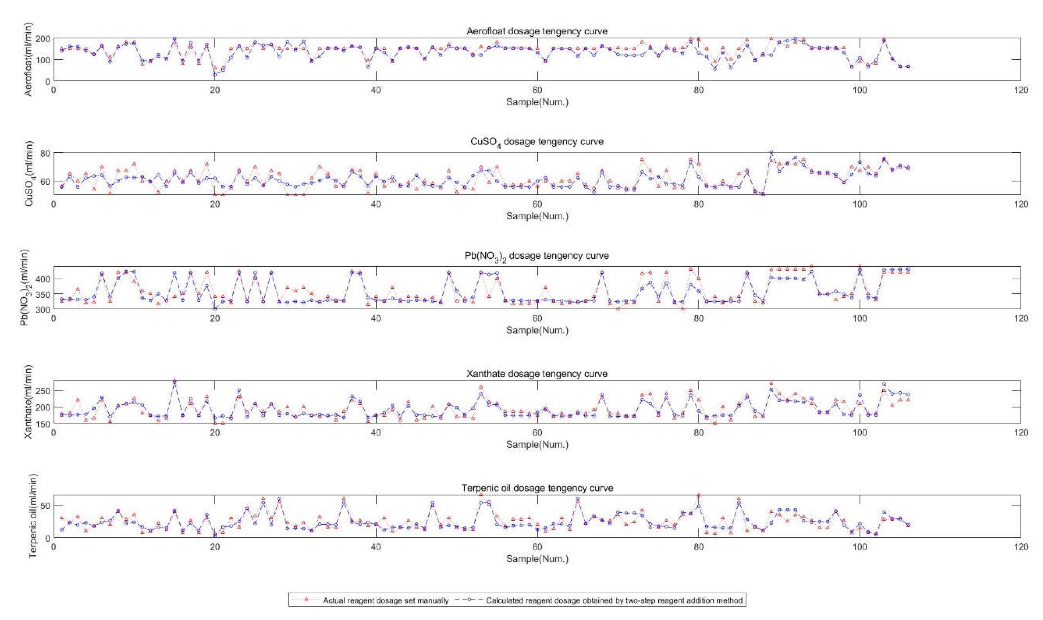
4.1.2. Validation of the Two-Step Reagent Addition Strategy

We tested the overall performance of the reagent addition optimal-setting control method. Taking the fifth rounds of the five-fold cross-validation experiments in antimony rougher flotation, the dosages of xanthate, aerofloat, CuSO₄, Pb (NO₃)₂, and terpenic oil using the STA–BRB rule base of reagent compensation (two-step reagent addition method) and the actual manually set values are shown in Figure 6.

Moreover, the MAEs between the manually set actual reagent addition and calculated reagent addition using the two-step reagent addition method are shown in

Table 12. The MAEs of reagent dosing using two-step reagent addition method.

Reagents	1st Fold	2nd Fold	3rd Fold	4th Fold	5th Fold	Average
Aerofloat	10.0498	17.3263	24.0008	21.6386	14.1372	17.4305 ± 5.0241
CuSO4	2.0468	3.0460	4.2893	5.2921	3.7765	3.6901 ± 1.0998
Pb (NO3)2	10.2426	16.1045	17.2852	19.4135	16.1904	15.8472 ± 3.0457
Xanthate	7.9539	15.1308	16.0834	20.5337	12.2117	14.3827 ± 4.1792
Terpenic oil	4.5212	5.4773	6.6492	12.5953	6.4852	7.1456 ± 2.8303

.

It is evident from Figure 6 and Table 12 that the calculated reagent dosages obtained from the two-step method generally match the actual reagent dosages. By using the two-step reagent addition method, the calculated reagent dosages became closer to the actual reagent dosages.

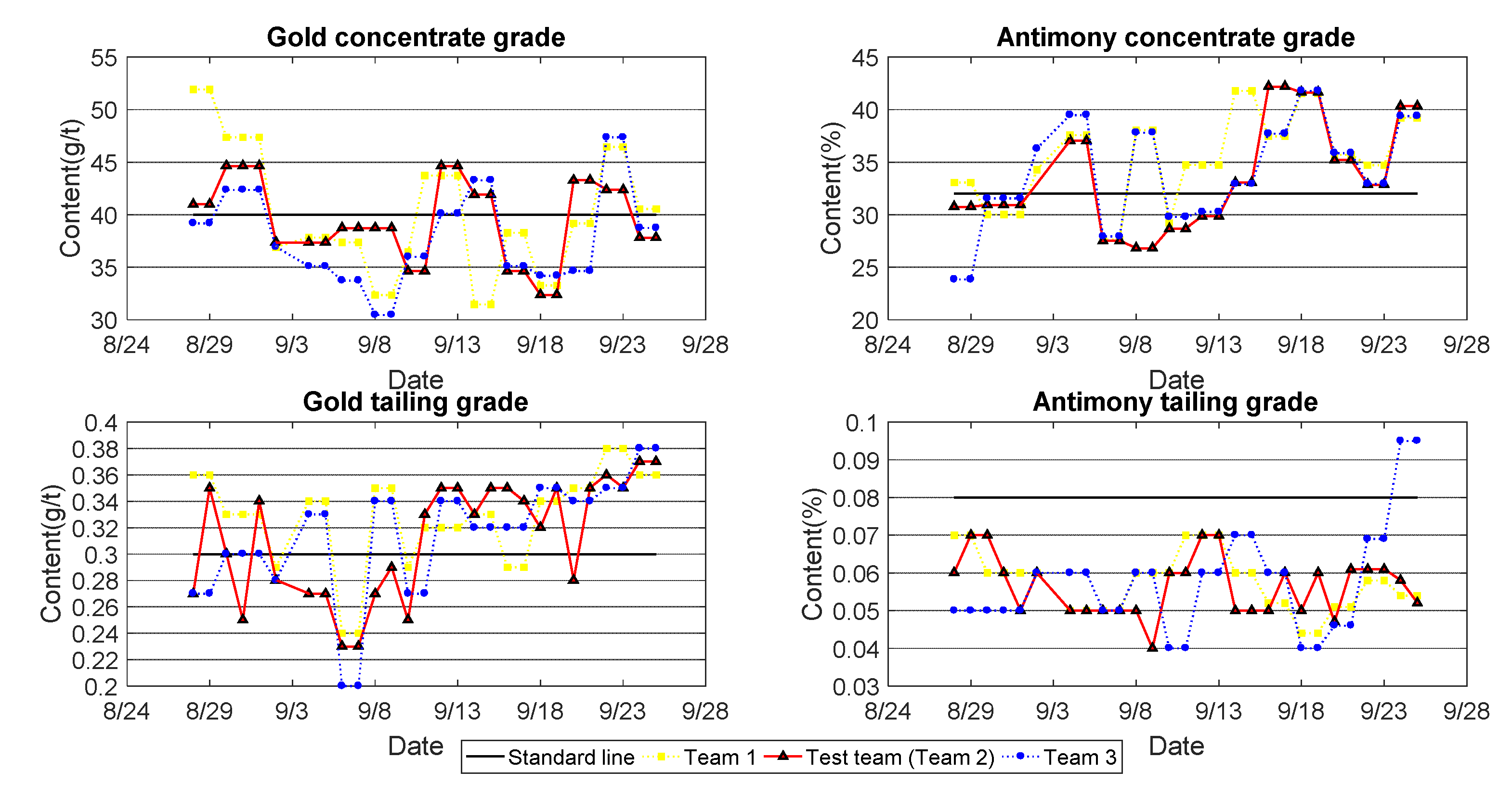
4.2. Industrial Test Results

Using the basic dosage pre-setting model based on RIMER and feedback reagent addition compensation model based on RBR, we implemented an automatic optimal-setting control for the gold-antimony flotation process and tested it in the froth image monitoring system of a gold-antimony flotation plant in Hunan province, China, which is shown in Figure 7.

In gold-antimony flotation production, every 24 h in a day is divided into three shifts, from 0:00 to 8:00 a.m., 8:00 a.m. to 4:00 p.m., and 4:00 to 12:00 p.m. The three shifts are managed by three separate teams. To ensure the reliability of the experimental results, we used a single shift test that lasted for an entire month, i.e., the automatic optimal-setting control system was applied when Team 2 (test team) was on shift. Members of Team 2 only needed to adjust the airflow rates and pulp levels, whereas Teams 1 and 3 used manual control. The feed ore was homogenized and stored in heaps, and each heap was usually used for one week. Thus, the feed grade was stable during the test and the process was under normal operations. Therefore, we can assume that the three teams were tested under the same conditions. The operating results, including concentrate and tailing grades, were compared between the automatic and manual systems. Monitoring results for the concentrate and tailing grade are shown in Figure 8. All technical indices of the three teams during the test are shown in

Table 13. Technical indices of each team.

	Technical Index	Team 1 Cumulative Mean Value	Test Team (Team 2) Cumulative Mean Value	Team 3 Cumulative Mean Value
Feed	Gold ore grade (g/t)	2.27	2.34	2.38
	Antimony ore grade (%)	1.60	1.55	1.61
Tailing and recovery	Gold recovery rate (%)	86.37	87.49	87.61
	Tailing gold content (g/t)	0.33	0.31	0.31
	Antimony recovery rate (%)	96.73	96.84	96.84
	Tailing antimony content (%)	0.05	0.05	0.05

.

As shown in Table 13, there was little difference between the cumulative mean values of gold ore grade and antimony ore ratios, meaning that the process ran under similar ore conditions for the three teams. From Figure 8 and Table 13, the indices of Team 2 are a little bit worse than those of Team 3, but better than the values of Team 1. That is, the automatic system can achieve similar performance to that of manual control. The automatic optimal-setting control of reagent addition can also help workers solve problems related to excessive reliance on human experience, tedious operations, and insufficient timeliness and accuracy.

However, there are still some issues that should be considered and improved. For example, in the rule inputs, only three or five referential points were used. To achieve more precise control of the process, more referential points should be considered. However, this will increase the scale of the rule base. Therefore, an optimized BRB needs to be further reduced, and the rule base for reagent compensation further refined, to achieve a more precise optimization method for reagent addition. Meanwhile, it would be better if the complexity of the reasoning process could be simplified.

5. Conclusions

Reagent addition is a decisive operating variable in the gold-antimony flotation process. According to principles of the flotation process and problems associated with current control of reagent addition and optimization, we proposed a two-step optimal-setting control strategy that included a basic dosage pre-setting model based on RIMER, and a feedback reagent addition compensation model based on RBR. The basic pre-setting model exploits the advantages of the RIMER approach to describe the complex relationships and uncertainty between the reagents and feed conditions. The composition model was based on froth image features and experiences of the operator. From the simulation, it was evident that the BRB and RIMER method has the advantage of describing the uncertainties and using a limited number of rules to solve a complex industrial problem. In an industrial setting, the method could be used to automatically control the process and lead to better performance. Finally, it should be mentioned that the rule model becomes more complicated with too many parameters. This aspect should be improved in future investigations.

References

1. Ata, S. Phenomena in the froth phase of flotation—A review. Int. J. Miner. Processing 2012, 102, 1–12. [Google Scholar] [CrossRef]
2. Bergh, L.G.; Yianatos, J.B. The long way toward multivariate predictive control of flotation processes. J. Process Control 2011, 21, 226–234. [Google Scholar] [CrossRef]
3. Moolman, D.W.; Aldrich, C.; Van Deventer, J.S.; Stange, W.W. Digital image processing as a tool for on-line monitoring of froth in flotation plants. Miner. Eng. 1994, 7, 1149–1164. [Google Scholar] [CrossRef]
4. Rath, S.S.; Sahoo, H.; Das, B. Optimization of flotation variables for the recovery of hematite particles from BHQ ore. Int. J. Miner. Metall. Mater. 2013, 20, 605–611. [Google Scholar] [CrossRef]
5. Azizi, D.; Gharabaghi, M.; Saeedi, N. Optimization of the coal flotation procedure using the Plackett–Burman design methodology and kinetic analysis. Fuel Process. Technol. 2014, 128, 111–118. [Google Scholar] [CrossRef]
6. Vieceli, N.; Durão, F.O.; Guimarães, C.; Nogueira, C.A.; Pereira, M.F.C.; Margarido, F. Grade-recovery modelling and optimization of the froth flotation process of a lepidolite ore. Int. J. Miner. Process. 2016, 157, 184–194. [Google Scholar] [CrossRef]
7. Wang, X.L.; Lu, M.Y.; Wei, S.M.; Xie, Y.F. Multi-objective optimization based optimal setting control for industrial double-stream alumina dige. J. Cent. South Univ. 2022, 29, 173–185. [Google Scholar] [CrossRef]
8. Chuk, D.; Kuchen, B.R. Supervisory control of flotation columns using multi-objective optimization. Miner. Eng. 2011, 24, 1545–1555. [Google Scholar] [CrossRef]
9. Barrozo, M.A.S.; Lobato, F.S. Multi-objective optimization of column flotation of an igneous phosphate ore. Int. J. Miner. Process. 2016, 146, 2–89. [Google Scholar] [CrossRef]
10. Jahedsaravani, A.; Marhaban, M.H.; Massinaei, M.; Saripan, M.I.; Noor, S.B. Froth-based modeling and control of a batch flotation process. Int. J. Miner. Process. 2016, 146, 90–96. [Google Scholar] [CrossRef]
11. Zhang, J.; Tang, Z.H.; Ai, M.X.; Gui, W.H. Nonlinear modeling of the relationship between reagent dosage and flotation froth surface image by Hammerstein-Wiener model. Miner. Eng. 2018, 120, 19–28. [Google Scholar] [CrossRef]
12. Zhu, J.; Gui, W.; Yang, C.; Xu, H.; Wang, X. Probability density function of bubble size based reagent dosage predictive control for copper roughing flotation. Control. Eng. Pract. 2014, 29, 1–12. [Google Scholar] [CrossRef]
13. Zhang, S.; Gao, X.W. A digital twin dosing system for iron reverse flotation. J. Manuf. Syst. 2022, 63, 238–249. [Google Scholar] [CrossRef]
14. Kaartinen, J.; Hätönen, J.; Hyötyniemi, H.; Miettunen, J. Machine-vision based control of zinc flotation-A case study. Control Eng. Pract. 2006, 14, 1455–1466. [Google Scholar] [CrossRef]
15. Xie, Y.; Wu, J.; Xu, D.; Yang, C.; Gui, W. Reagent Addition Control for Stibium Rougher Flotation Based on Sensitive Froth Image Features. IEEE Trans. Ind. Electron. 2017, 64, 4199–4206. [Google Scholar] [CrossRef]
16. Cao, B.F.; Xie, Y.F.; Yang, C.H.; Gui, W.H.; Li, J.Q. Reagent Dosage Control for the Antimony Flotation Process Based on Froth Size Pdf Tracking and an Index Predictive Model. J. Min. Sci. 2019, 55, 452–468. [Google Scholar] [CrossRef]
17. Yang, J.B.; Liu, J.; Wang, J.; Sii, H.S.; Wang, H.W. Belief rule-base inference methodology using the evidential reasoning approach-RIMER. IEEE Trans. Syst. Man Cybern.-Part A: Syst. Hum. 2006, 36, 266–285. [Google Scholar] [CrossRef]
18. Yang, J.B. Rule and utility based evidential reasoning approach for multi-attribute decision analysis under uncertainties. Eur. J. Oper. Res. 2001, 131, 31–61. [Google Scholar] [CrossRef]
19. Yang, J.B.; Xu, D.L. On the evidential reasoning algorithm for multiple attribute decision analysis under uncertainty. IEEE Trans. Syst. Man Cybern.-Part A: Syst. Hum. 2002, 32, 289–304. [Google Scholar] [CrossRef]
20. Ignatkina, V.A.; Shepeta, E.D.; Samatova, L.A.; Bocharov, V.A. An Increase in Process Characteristics of Flotation of Low-Grade Fine-Disseminated Scheelite Ores. Russ. J. Non-Ferr. Met. 2020, 60, 609–616. [Google Scholar] [CrossRef]
21. Geng, Z.X.; Chai, T.Y.; Yue, H. A method of hybrid intelligent optimal setting control for flotation process. In Proceedings of the 2008 7th World Congress on Intelligent Control and Automation, Chongqing, China, 25–27 June 2018; pp. 4713–4718. [Google Scholar]
22. Chen, Y.W.; Yang, J.B.; Xu, D.L.; Zhou, Z.J.; Tang, D.W. Inference analysis and adaptive training for belief-rule based systems. Expert Syst. Appl. 2011, 38, 12845–12860. [Google Scholar] [CrossRef]
23. Yang, C.H.; Zhou, K.J.; Mou, X.M.; Gui, W.H. Froth color and size measurement method for flotation based on computer vision. Chin. J. Sci. Instrum. 2009, 30, 717–721. (In Chinese) [Google Scholar]
24. Han, J.; Yang, C.H.; Zhou, X.J.; Gui, W.H. A two-stage state transition algorithm for constrained engineering optimization problems. Int. J. Control. Autom. Syst. 2018, 16, 522–534. [Google Scholar] [CrossRef]
25. Nair, V.; Hinton, G.E. Rectified linear units improve restricted Boltzmann machines. In Proceedings of the International Conference on Machine Learning, Haifa, Israel, 21–24 June 2010; pp. 807–814. [Google Scholar]
26. Sun, Y.; Wang, X.; Tang, X. Deeply learned face representations are sparse, selective, and robust. In Proceedings of the IEEE Conference on Computer Vision and Pattern Recognition, Boston, MA, USA, 7–12 June 2015; pp. 2892–2900. [Google Scholar]
Figure 1. Process diagram of gold-antimony flotation.
Processes 10 01933 g001
Figure 2. Reagent addition optimal-setting control strategy for gold-antimony flotation process.
Processes 10 01933 g002
Figure 3. Framework of optimal learning model for BRB system.
Processes 10 01933 g003
Figure 4. Probability statistical distributions of optimal froth image features.
Processes 10 01933 g004
Figure 5. Froth image when the froth features are at the optimal intervals.
Processes 10 01933 g005
Figure 6. Comparison of the two methods for reagent dosing.
Processes 10 01933 g006
Figure 7. Hardware structure of froth image monitoring system.
Processes 10 01933 g007
Figure 8. Monitoring results of concentrate and tailing grade.
Processes 10 01933 g008