Abstract
Osteoporosis is still a serious public health issue in Thailand, particularly in postmenopausal women; meanwhile, new effective screening tools are required for rapid diagnosis. This study constructs and confirms an osteoporosis screening tool-based decision tree (DT) model. Four DT algorithms, namely, classification and regression tree; chi-squared automatic interaction detection (CHAID); quick, unbiased, efficient statistical tree; and C4.5, were implemented on 356 patients, of whom 266 were abnormal and 90 normal. The investigation revealed that the DT algorithms have insignificantly different performances regarding the accuracy, sensitivity, specificity, and area under the curve. Each algorithm possesses its characteristic performance. The optimal model is selected according to the performance of blind data testing and compared with traditional screening tools: Osteoporosis Self-Assessment for Asians and the Khon Kaen Osteoporosis Study. The Decision Tree for Postmenopausal Osteoporosis Screening (DTPOS) tool was developed from the best performance of CHAID’s algorithms. The age of 58 years and weight at a cutoff of 57.8 kg were the essential predictors of our tool. DTPOS provides a sensitivity of 92.3% and a positive predictive value of 82.8%, which might be used to rule in subjects at risk of osteopenia and osteoporosis in a community-based screening as it is simple to conduct.
1. Introduction
Osteoporosis is considered a severe public health issue in Thailand since it can result in fractures that leave people bedridden and immobile and eventually lead to illness, including chronic diseases of the respiratory system, pressure ulcers, urinary tract inflammation infection, and possibly death. Osteoporosis is a disease of the bone characterized by a decrease in bone mass and changes in bone structure, leading to an increased risk of fractures [1]. In the population more than 50 years of age, osteoporosis is more common, occurring in 33% of females and 20% of males, due to the lack of estrogen in women after menopause, reducing calcium binding to the bone tissue. The WHO reports that osteoporosis occurs in 1/3 of women aged 60–70 and 2/3 aged 80 [2,3]. Diagnosing and treating patients with osteoporosis are expensive. The estimated annual cost per patient for hip fracture care is THB 116,459, of which the direct cost per patient is THB 59,881 [4]. Dual-energy X-ray absorptiometry (DEXA) for bone mineral density assessment is the gold standard for diagnosing osteoporosis and consistently predicting the risk of fractures caused by osteoporosis [1]. However, Thailand still has a shortage of DEXA bone density scanners. Most bone density scanners are available at university hospitals, private hospitals, hospitals in Bangkok, and some center hospitals. Therefore, most patients with osteoporosis are undiagnosed because early osteoporosis is asymptomatic. Only after fractures have occurred will patients be admitted for treatment and assessment. Some health care institutions employ heel-to-head ultrasound (QUS), which is affordable, quick, and simple to obtain but has limited sensitivity and cannot replace a conventional instrument [5]. Therefore, osteoporosis risk screening criteria are used before considering whether the patients should be referred for examination with DEXA, which will assist with reducing the cost of effective screening in the limited resource and rural areas. In 2001, the risk of osteoporosis in Asian countries was studied, and the formula for determining the risk of osteoporosis, known as the OSTA (Osteoporosis Self-Assessment for Asians) index, was obtained: 0.2 × (weight-age), with body weight in kilograms and age in years [6]. In addition to OSTA screening, there is a Khon Kaen Osteoporosis Study (KKOS) score method [7] that combines the scores from age (year) and weight (kg) and interprets the results as follows: KKOS less than −1 indicates a high risk of developing osteoporosis and KKOS greater than −1 shows a low risk of developing osteoporosis.
The OSTA index and KKOS score were obtained from the conventional mathematic modeling of the univariate models and logistic regression methods based solely on age and weight factors. More recent tools have also been developed for a specific population of Chinese that also used age and weight as predictors using the formula weight (kg) − (2 × age (year)) + 50 [8]. In addition to these tools, the WHO conducted a population-based cohort study in Europe, North America, Asia, and Australia. The FRAX® without bone mineral density (BMD) tool was developed to assess the likelihood of fractures due to osteoporosis in the next decade. The clinical risk associated with BMD was considered, as femoral neck BMD was related to BMI based on age, sex, weight, height, and clinical risk. A modified-FRAX® Thai was developed using the Thai standard value, but inputting variables in the tool is complicated, making it potentially unsuitable for common use [9,10]. Other tools created from the conventional mathematic-based methods since the years of 1998–2002 for classifying the risk of osteoporosis or bone fracture in peri/postmenopausal women include ABONE (predictive variables: age, weight, estrogen) [11], ORAI (predictive variables: age, weight, estrogen) [12], OSIRIS (predictive variables: age, weight, hormone therapy, impact fracture) [13], SCORE (predictive variables: age, weight, race, rheumatoid arthritis, previous fracture, hormone therapy) [14], and SOFSURF (predictive variables: age, weight, smoking, history of fracture) [15]. All of these required some parameters, including estrogen use history, that could be missing due to no data record of the risk population or could not be measured in a limited resource.
Recently, data science has come into play in the medical field by assisting in forecasting disease risk more accurately than traditional methods. As established in a previous study conducted outside Thailand, osteoporosis screening using data science methods is successful for data analysis, highly accurate in predicting osteoporosis risk in postmenopausal women and capable of identifying risk variables linked with osteoporosis [16,17,18,19,20,21]. A decision tree (DT) is one example of a machine learning technology dealing with data analysis with a small assumption. Its primary objective is to perform different classification tasks and establish decision rules. Although some studies have used DT in medicine to perform disease diagnoses [22,23], most of them were according to a single DT algorithm, most frequently C4.5, or just compared with other machine learning algorithms [24,25]. Presently, few researchers have used algorithms such as classification and regression tree (CART); chi-squared automatic interaction detection (CHAID); and quick, unbiased, efficient statistical tree (QUEST) on project case studies and comprehensive analyses of rule characteristics and classification results. Other machine learning algorithms, including support vector machines, random forests, logistic regression, artificial neural network, and eXtreme Gradient Boosting, can also be used for classification predictions, but their results are challenging to interpret [26,27]. Instead, DT is a type of machine learning algorithm and analysis technique that can be used to construct models quickly, perform predictions, identify patterns and rules in data, and process large amounts of data.
In this study, we hypothesized that in comparison with the traditional screening tools, a decision tree-based model could be accessed with high sensitivity sufficient to enhance the screening of osteopenia and osteoporosis in the era of machine learning algorithms for postmenopausal Thai women.
2. Materials and Methods
2.1. Data Collection
We retrospectively collected the data from the electronic health records of postmenopausal Thai women at the department of obstetrics and gynecology, Ramathibodi Hospital, Bangkok. The inclusion criteria were postmenopausal women with anatomy suitable for evaluation by DEXA of the total bone mass density, ability to read and give informed permission, and readiness to participate in the study. The following were listed as exclusion criteria: history or evidence of metabolic bone disease (other than postmenopausal bone loss), presence of cancer with known metastasis to bone, evidence of significant renal impairment, removal of the ovary, previous fracture or replacement of both hips, and prior treatment with any bisphosphonate, fluoride, or calcitonin [6]. Total BMD was assessed by DEXA (Lunar Prodigy, New York, NY, USA) scanning. The definitive diagnosis of osteoporosis was based on WHO criteria [1]. Briefly, participants with a BMD T-score ≤ −2.5 standard deviation (SD) below the normal were considered to have osteoporosis, whereas a BMD T-score between −1 and −2.5 SD was classified as osteopenia. A BMD T-score ≥ −1.0 SD was considered normal. Overall, 266 abnormal (BMD T-score < −1.0 SD; osteopenia/osteoporosis subjects) and 90 normal (BMD T-score ≥ −1.0 SD) postmenopausal women were included in the study. We enrolled 11 simple biographical and anthropometric variables as possible presumptive variables in a model because these variables do not require a special instrument to measure but only require well-trained people to collect accurate results. A simple variable is more suitable as a screening variable in a field population. No missing information was observed for age, weight, and height, while the percentage of missing values in other variables was not more than 5 in both the normal and abnormal groups. Characteristics of the study’s variables are presented in Table 1.

Table 1.
Characteristics of the predictive variables.
2.2. Experimental Design
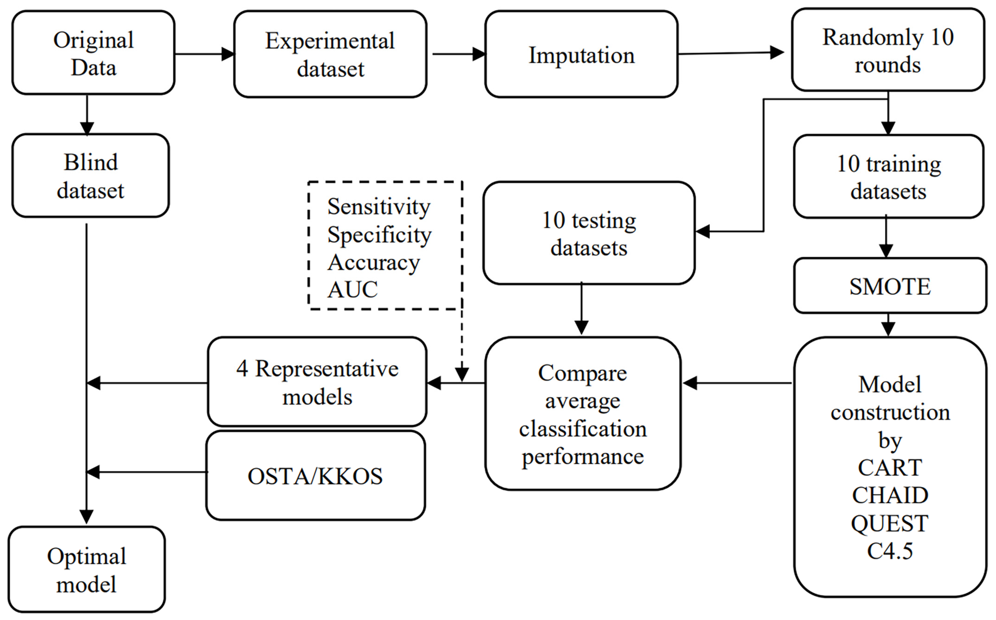
This study proposes a tool for the high-performance screening of osteoporosis risk using a DT. First, as shown in Figure 1, the initial data are categorized into experimental and blind datasets. The missing information in the experiment dataset is treated using k-nearest neighbor imputation before being split into the training and testing datasets randomly in 10 rounds in Python. Furthermore, the Synthetic Minority Oversampling Technique (SMOTE) technique treats the imbalance problem in normal and abnormal groups. The CART, CHAID, QUEST, and C4.5 algorithms are then applied to develop models for 10 datasets. The average accuracy, sensitivity, specificity, and AUC are calculated for 10 models using the testing dataset for each algorithm and subsequently compared. A representative model out of 10 is selected for each machine learning technique, considering the highest accuracy, sensitivity, specificity, AUC, and possibility of implementing the model. The blind dataset is used with the four representative models and compared with the conventional OSTA and KKOS tools, and subsequently, the optimal model is selected.
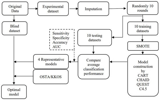
Figure 1.
Model construction and validation using machine learning algorithms.
2.3. Data Preparation
We preprocessed the experimental data, which involved missing data handling, randomly separated them into 10 training and testing datasets, and balanced the training datasets before conducting model construction.
2.3.1. Missing Data Handling
The primary set of predictor variables was subjected to Little’s missing completely at random (MCAR) test. The results showed that missing values were MCAR for the dataset, accounting for p-value = 1.00. A single imputation was employed in the dataset to fill in the missing data. The k-nearest neighbor approach accounted for all predictor factors for imputation, excluding the outcome variable.
2.3.2. Training and Testing Data
We randomized 10 rounds to achieve 10 datasets to ensure the lowest bias by chance in the randomization. The experimental data were separated into training and testing sets following imputation. The training set included 80% of the data for model development, and the testing set consisted of the remaining 20% for internal model validation.
2.3.3. Imbalanced Data Handling
Most well-known machine learning algorithms perform best when the distribution of positive and negative examples is balanced, and even DTs experience issues when the dataset is unbalanced. In these situations, DT models frequently produce results with higher accuracy in most classes. Several studies have shown the benefits of SMOTE for addressing uneven data sets [28,29]. Therefore, for this evaluation, we used SMOTE to balance the data between the majority presented in the abnormal group (experimental dataset, n = 240) and the minority class presented in a normal group (experimental dataset, n = 81).
2.4. DT Algorithms
2.4.1. CART Algorithm
CART is a recursive partitioning algorithm applied to classification and regression. The technique entails repeatedly separating subsets of the dataset into two child nodes using all attributes, starting with the complete dataset. The best feature is selected according to diversity measures (Gini, twoing, ordered twoing, and least-squared deviation) [30]. Here Gini’s impurity for categorical target variables was used.
The Gini’s impurity index of a training set D is defined as follows:
where represents the probability that an instance in D be underclass (for i = 1, 2,…, m) and is calculated by .
The Gini index considers a binary split for each attribute A, which is categorized into and . The Gini index of D, according to the partition, is
The reduction in impurity that binary spit would gain on attribute A is the following:
The attribute that maximizes the reduction in impurity (i.e., has the minimum Gini index) is selected as the splitting attribute [31].
2.4.2. QUEST Algorithm
QUEST is a binary DT algorithm that can be used for data mining and classification. For each split, the algorithm computes the relationship between each input attribute and each target attribute using the ANOVA F-test, Levene’s test (for ordinal and continuous attributes), or Pearson’s chi-square (for nominal attributes). Using two-means clustering, two super-classes are created if the target attribute is multinomial. It is decided which feature will be split based on which one has the strongest correlation with the target attribute. For the input attribute, the best splitting point is determined using quadratic discriminant analysis. Ten-fold cross-validation is performed to prune the trees [32].
2.4.3. CHAID Algorithm
Kass [33] originally proposed the CHAID algorithm. The algorithm is used to determine whether there is a correlation between a categorical dependent variable and several independent variables that could be categorical, numerical, or both. However, the coding and transformation into categorical variables should be finished in advance for numerical variables. The CHAID algorithm is based on a criterion that recursively categorizes the heterogeneous input data set into homogenous groups regarding the dependent variable categories. The Pearson’s chi-square statistic is used as a criterion for division. The procedure for testing and expressing conclusions is similar to the traditional approach for statistically testing hypotheses. The algorithm is conducted in two steps: merging and splitting.
The nonsignificant categories for each independent variable were combined in the merging step. Each independent variable’s final category would lead to a separate child node if the independent variables were used to divide the node. The two variable types with the highest p-values regarding the dependent variable were the most comparable, so they were combined. If no new merging couples are found, or if the p-value for all prospective pairs is less than the specified significance level, the search is continued. The corrected p-value is also computed to apply it in the splitting stage. The p-value is calculated for the merged categories when nonbinary independent variables are used using the Bonferroni adjustment.
The independent variable that will split into the best nodes is determined by comparing the modified p-values associated with each variable. If the adjusted p-value is less than or equal to the significance threshold, the node is categorized into sub-nodes based on the merged categories. If not, the node is considered the terminating node. When all the independent variables in the input have p-values greater than the assigned split threshold, the tree-building procedure ends. When a value is missing, CHAID addresses it by treating every missing value as a valid independent category. CHAID does no pruning.
2.4.4. C4.5 Algorithm
C4.5 is a supervised learning algorithm that uses a splitting criterion known as a gain ratio. The attribute selected as the splitting attribute has the highest gain ratio [31]. Given that a training set D has m distinct values for the class label attribute (for i = 1, 2,…, m). The notations and denote the number of instances in and , respectively. If the cases in are categorized into ν groups according to the values of attribute A as shown in the training data, A splits D into partitions for j = 1, 2,…,ν.
The information gain is defined as the following:
where is the expected information and is the expected information needed to categorize an instance from D based on the partitioning by A.
The gain ratio of A is presented as follows:
2.5. Model Construction and Selection
In this study, we implemented four DT algorithms, CART, CHAID, QUEST, and C4.5, to the training and testing dataset. Each algorithm was run 10 times according to 10 training and testing datasets. Average accuracy, sensitivity, specificity, and AUC were compared. Each algorithm’s representative models were selected according to the best performance, expert knowledge, and possible application. To identify the final optimized model, these 4 selected models were then tested by 35 samples of the blind dataset to achieve the most effective model. The traditional tools OSTA and KKOS were used to compare (Figure 1). Positive predictive value (PPV) and negative predictive value (NPV) were also selected as criteria in this step. For CART, QUEST, and CHAID, we initially ranged the maximum tree depth from 2 to 5, with fixed values for the minimum number of cases in parent and child nodes of 100 and 50, respectively. Likewise, a confidence factor was set between 0.05 and 0.25 in increments of 0.05, and a minimum number of objects was set between 2 and 20 in increment of 2. The optimal model of each algorithm was selected based on the initial high performance of the preliminary testing and simple interpretation. The hyperparameters and conditions used for each algorithm are presented in Table 2. The performance criteria that were used in the study were calculated as follows:

Table 2.
Using the hyperparameters of the four algorithms.
- Accuracy = (TP + TN)/(TP + TN + FP + FN)
- Sensitivity = TP/(TP + FN)
- Specificity = TN/(TN + FP)
- Positive Predictive value (PPV) = TP/(TP + FP)
- Negative predictive value (NPV) = TN/(TN + FN)
where TP represents an outcome in which the model correctly predicts the osteoporosis class, TN represents an outcome in which the model correctly predicts the normal class, FP represents an outcome in which the model incorrectly predicts the osteoporosis class, and FN represents an outcome in which the model incorrectly predicts the normal class.
2.6. Statistical Analysis
A normality test was applied to all continuous variables. The mean and SD were computed for the normally distributed data, whereas median and interquartile range (IQR) values were calculated for non-normal distribution data. An independent t-test or Mann–Whitney test was used to test the differentiation between the two comparative groups as appropriate. In the case of more than two group comparisons, one-way ANOVA was used to compare the differences. A p-value less than 0.05 was considered a significant difference.
3. Experimental Results
3.1. General Characteristics and the Difference in Parameters between the Normal and Abnormal Groups
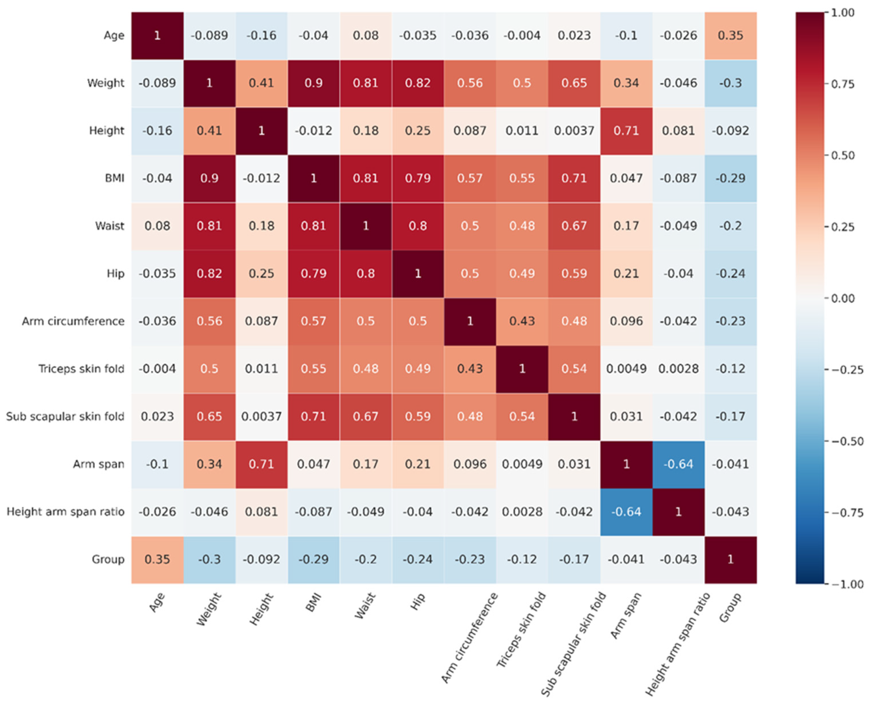
We proposed statistical analysis to initially notice the likelihood of the difference in each parameter between the normal and abnormal groups. The results revealed that among biography and anthropometric features, most features represent significant differences except for height, arm span, and height arm span ratio (Table 3). The most correlated features with osteoporosis status were age and weight (Figure 2). Even though not all significant differences in features were found, we included all the features to perform DT analysis because they may be included in a model tested by different decision tree algorithms as machine learning algorithms have overcome the limitations of statistical-based testing. DT algorithms construct splits on single features that improve classification based on an impurity measure like Gini or entropy [34,35].

Table 3.
Characteristics of the parameters in the normal and abnormal groups.

Figure 2.
The correlation matrix of features and group.
3.2. Performance of Four Decision Tree Algorithms and the Selected Model
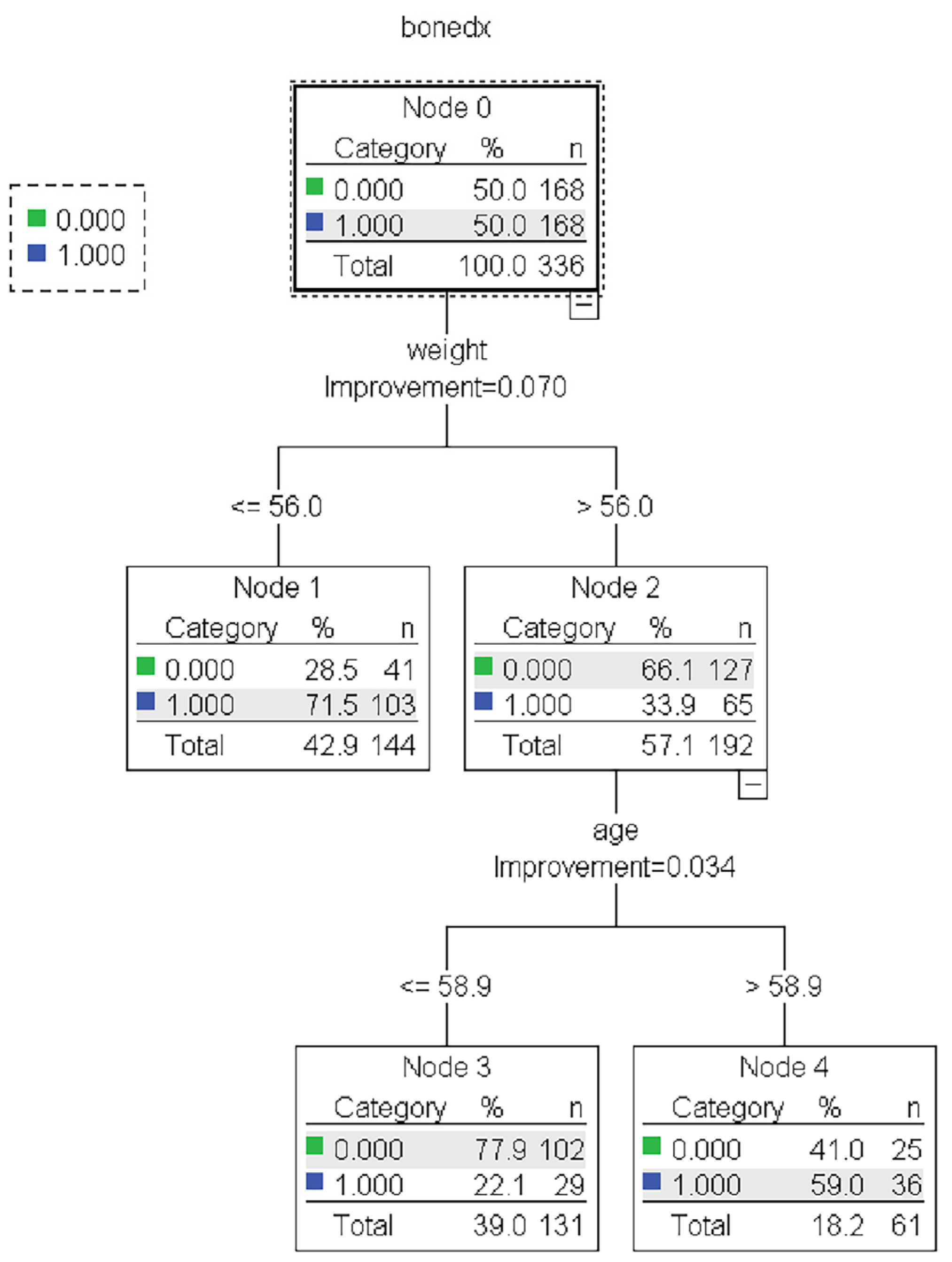
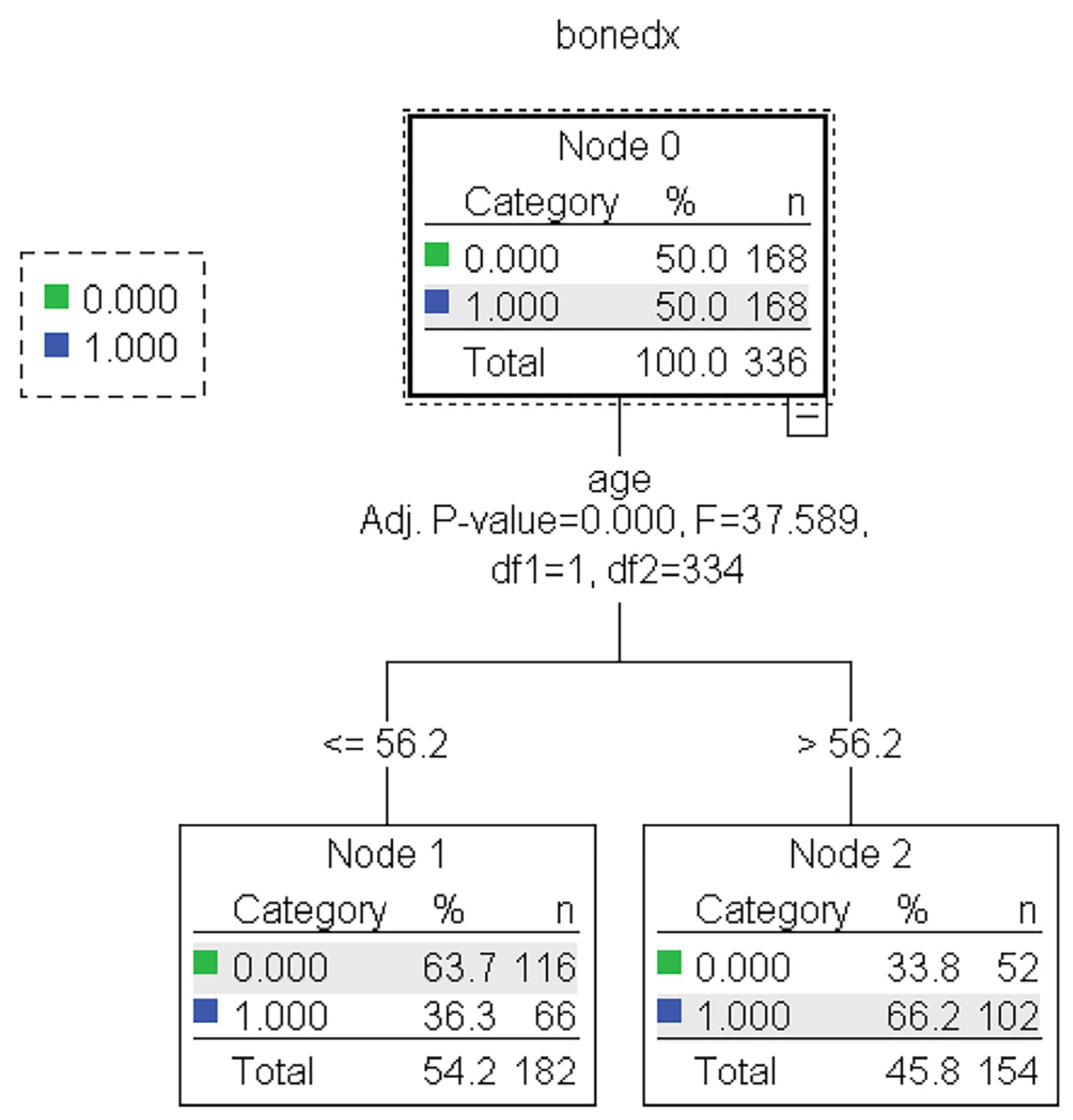
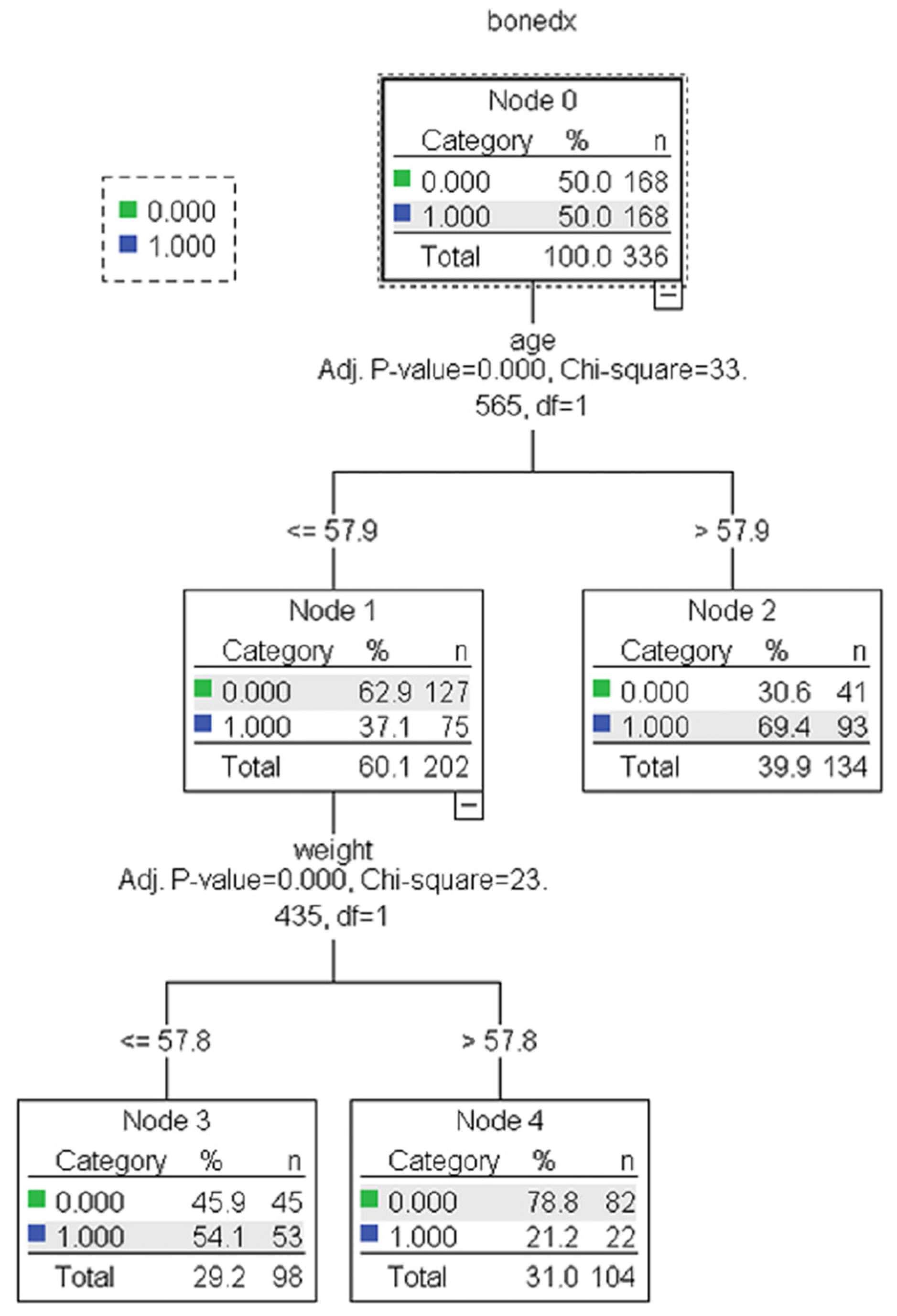
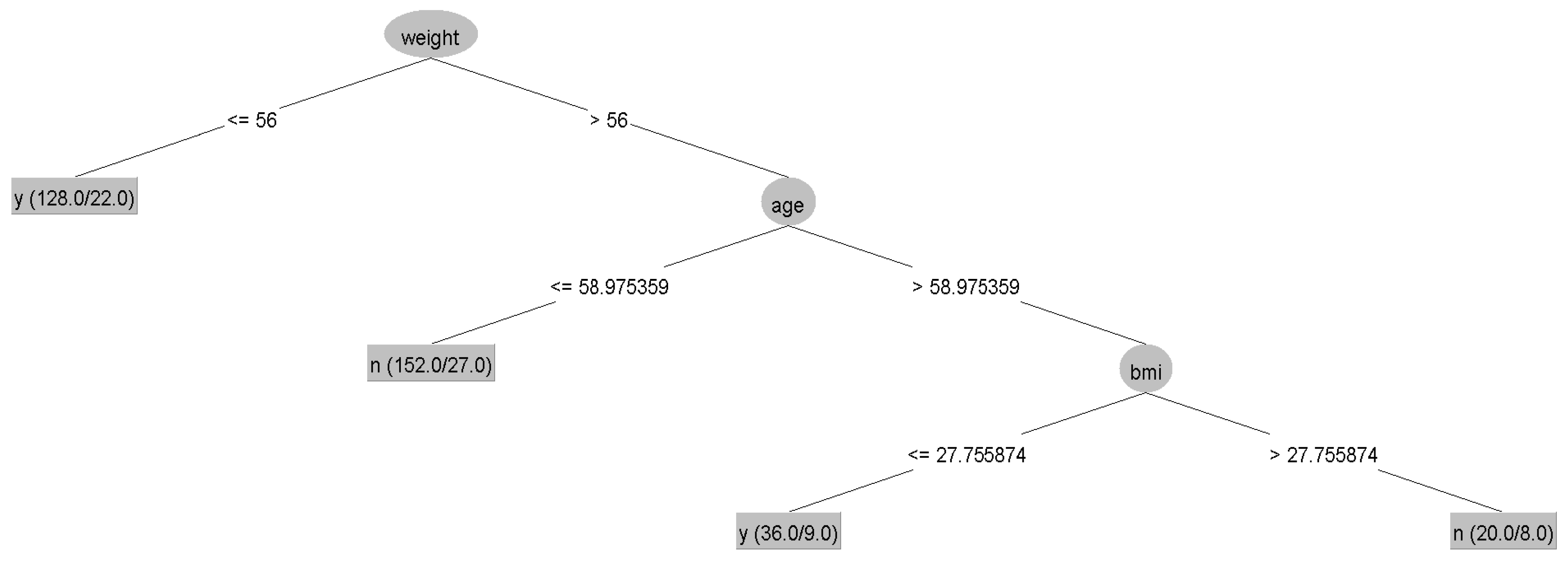
The results showed no statistically significant differences in the average accuracy, sensitivity, specificity, or AUC of the four DT algorithms (p-value > 0.05). Each algorithm presented distinct characteristics. The highest accuracy, sensitivity, specificity, and AUC were found in the CART, C4.5, QUEST, and CHAID algorithms, respectively (Table 4). For each machine learning algorithm, the best model was selected among 10 models considering the testing dataset’s highest accuracy, sensitivity, specificity, and AUC and the possibility of implementing the model. The performance of the representative model for CART, CHAID, QUEST, and C4.5 is presented in Table 5. Among the 4 representative models, CHAID produces the highest accuracy (0.804) and sensitivity (0.875), whereas QUEST expresses the highest specificity (0.880) and AUC (0.773). The representative trees for CART, CHAID, QUEST, and C4.5 are shown in Figure 3, Figure 4, Figure 5 and Figure 6, respectively. Weight and age are the most vital features in CART and CHAID, whereas age is an essential attribute in QUEST. The most critical parameters for the C4.5 algorithm are weight, age, and BMI. For CART, QUEST, CHAID, and C4.5, the depth levels of the tree model are 2, 1, 2, and 3, respectively.

Table 4.
The performance of the four algorithms.

Table 5.
The performance of the representative models for CART, CHAID, QUEST, and C4.5.
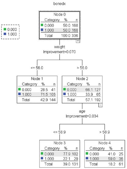
Figure 3.
The representative models of the CART algorithm. Normal and abnormal groups are indicated by 0 and 1, respectively. There are 336 records with a balance of normal and abnormal groups for model construction, as shown in node 0 of the CART tree.
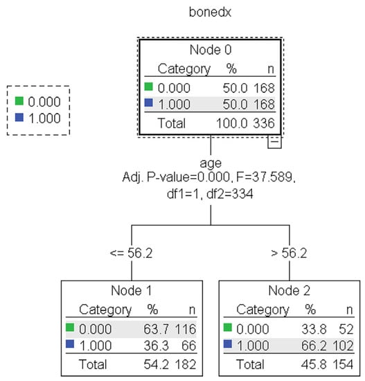
Figure 4.
The representative models of the QUEST algorithm. Normal and abnormal groups are indicated by 0 and 1, respectively. There are 336 records with a balance of normal and abnormal groups for model construction, as shown in node 0 of the QUEST tree.
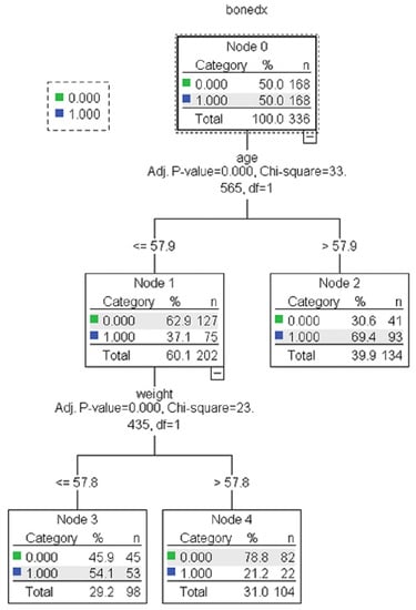
Figure 5.
The representative models of the CHAID algorithm. Normal and abnormal groups are indicated by 0 and 1, respectively. There are 336 records with a balance of normal and abnormal groups for model construction, as shown in node 0 of the CHAID tree.
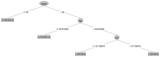
Figure 6.
The representative models of the C4.5 algorithm.
3.3. Blind Data Testing, Final Model Selection and Rule Extraction
The blind records of 35 postmenopausal women were tested using the 4 representative models as shown in Figure 3, Figure 4, Figure 5 and Figure 6 and traditional approach tools, such as OSTA and KKOS (Table 6). As presented in Table 7, the highest accuracy (0.800) and sensitivity (0.923) are provided by the CHAID algorithm, whereas the specificity for CART, CHAID, and C4.5 are comparable. Additionally, the OSTA and KKOS indicated the highest specificity (0.889). The positive predictive value (PPV) and negative predictive value (NPV) range from 0.808 to 0.938 and 0.348 to 0.667, respectively. Regarding health care, detecting the risk of osteoporosis in postmenopausal women is more important than detecting normal patients. Hence, we chose CHAID’s tree model because it has the best sensitivity and PPV for detecting risk in postmenopausal women. The rule was extracted from the tree model of the representative CHAID algorithm, as presented in Table 8. We named our model the Decision Tree for Postmenopausal Osteoporosis Screening (DTPOS).

Table 6.
Classifications for the 35 records of postmenopausal women using the 4 representative models as well as the OSTA and KKOS approaches. Normal and abnormal groups are indicated by 0 and 1, respectively.

Table 7.
Performance of the selected models and comparison with OSTA and KKOS in the blind data.

Table 8.
Decision Tree for Postmenopausal Osteoporosis Screening (DTPOS) rule.
4. Discussion
Studies on the prevalence of osteoporosis in hospitalized Thai women at Thai government hospitals and random surveys of women in every region of Thailand in 2008 and 2011 indicate that 11%–13% of women over 40 are assumed to have femoral neck osteoporosis, and 19%–21% of them have lumbar spine osteoporosis [36,37]. It was reported in 2015 that people with osteoporotic hip fractures in the northern part of the country had higher death rates and other relevant characteristics. In the first year, the average death rate was 21.1%, which was 9.3 times higher than the general population rate. At the end of the 10th year, 68% of people had died [38]. These data showed that osteoporosis is a primary life-threatening condition and a major problem in the country. Therefore, early screening and diagnosis are crucial. Numerous screening tools have been developed with the same goal of identifying the risk population to the entrance to BMD measurement to prevent future bone fracture. Among the screening tools, KKOS, OSTA, and FRAX® are the most frequently referred to in Thailand, as suggested by the Thai Osteoporosis Foundation [37,39]. The prevalence of osteoporosis and hip fracture has not significantly decreased since the tools’ implementation and validation. Furthermore, the number of osteoporosis-related fractures, the expense of health care related to fractures, and post-fracture mortality were all predicted to increase as Thailand’s elderly population (those 60 and older) increases from 14% of the total population in 2015 to approximately 30% by 2050 [40,41,42,43]. Therefore, alternative tools with high sensitivity are required to support different approaches.
The traditional screening tools were mainly developed based on mathematical assumptions that prevent the critical finding of the predictive variables or event from alternate the cutoff point of the variable because the statistical model used had a strict assumption. In the new era of data science, machine learning algorithms have been developed and have overcome the limitation of mathematical and statistical-based modeling [34,35]. Our study found that the DT approach could also identify the predictive variables. The most crucial variables were age and weight, which also agree with several current statistical and machine learning-based tools [8,9,10,11,12,13,14,15,16,18,19,20,21]. We noticed the highest performance with CHAID algorithm, so its representative tree was then used to extract the rule, namely, DTPOS. Postmenopausal women over age 58 have a BMD T-score < −1.0 as the predicting condition of osteopenia or osteoporosis. Postmenopausal women whose age is less than or equal to 58 and weight less than 57.8 kg also have a BMD T-score < −1.0, while those whose weight is more than 57.8 kg are considered to have a BMD T-score ≥ −1.0 or predicted to be in the normal group.
Compared with the KKOS and OSTA in the blind dataset testing, which represent the same age and weight variables in the model, the DTPOS model has the highest accuracy, sensitivity, and NPV. In contrast, the specificity of DTPOS is not very high, although its PPV is comparable. These findings showed that the DTPOS model could identify more osteopenia and osteoporosis in postmenopausal women. For instance, in the disagreement prediction of the 13 abnormal cases (No. 4, 5, 7, 9–11, 17, 19–21, 25, and 29–30), DTPOS correctly forecasted all 13 cases as abnormal, whereas OSTA missed all 13 cases and KKOS missed 9 cases. The performance difference could be due to the different methods used in model construction that provide the different cutoff levels. Overall, KKOS sensitivity and specificity in the validation cohort are 70% and 73%, respectively [43]. Furthermore, the OSTA model is based on the recruitment of samples from many nations, making it non-nation-specific. Different tools based on different construction methods have their own potential and characteristics for classification [20,44]. Implementing different models in various nations results in several performances because of the different body sizes, lifestyles, environmental, and genetic factors. Nine screening tools were evaluated in both men and women among community-dwelling older people in Taiwan. Of these techniques, 6 could deliver up to 100% sensitivity; however, the specificity was not satisfied [45]. A comparison of 6 osteoporosis risk assessment tools among postmenopausal women in Kuala Lumpur, Malaysia, indicated that SCORE had the best balance between recall (1.00), precision (0.04–0.12), and AUC (0.072–0.161) [46]. In middle-aged Thai women, FRAX® without BMD, SCORE, and OSTA have appropriate validity as tools for ruling out osteoporosis with a specificity of more than 75%; however, the sensitivity range is only 1.43–57.33% [4]. For other Asian countries, including Vietnam, OSTA and the osteoporosis screening tool for Chinese (OSTC) were evaluated in the community for osteoporosis screening. OSTA and OSTC were useful self-assessment tools for osteoporosis detection in postmenopausal Vietnamese women. The highest levels of OSTA’s sensitivity and specificity were 74.6% and 81.4%, compared with 73.9% and 82.6% for OSTC [47].
These previous studies show that specific new development tools are required in particular populations to enhance the sensitivity of osteoporosis findings. Our DT machine learning approach could provide a simple rule that is very easy to use, particularly for use in community-based screening. Very high sensitivity, up to 92.3%, showed that our tool could be used to assess the risk of osteopenia and osteoporosis. The village health volunteers can use the tool without any training and with greater frequency. Self-screening is also simple for those with access to a weighted scale and a measuring tape. In the case of those at a risk of osteoporosis, the volunteer or people themselves can immediately change their behavior or lifestyle to reduce the risk of bone fracture and consult a doctor for an osteoporosis diagnosis.
The DTPOS rule recruits a sample from a specific postmenopausal Thai population from only one hospital. The results may not be generalizable for all postmenopausal women in other areas who have distinct biological characteristics. The application’s usage may also be limited in other nations. Although it provides high sensitivity, PPV, and NPV, the specificity is not high enough. The use of the tools is necessary to consider some missing classifications. Because the model was not assessing the performance of people with a high risk of osteoporosis, such as people with a history of fractures, clinical risk factors, lifestyle habits (i.e., smoking and alcohol assumption), estrogen therapy, nutritional status (i.e., vitamin D levels), and genetic predisposition factors, which were reported to affect bone mass density [48,49,50,51], future studies are required to enhance the model’s performance and investigate it in a large study and different settings.
5. Conclusions
We used DT machine learning algorithms to search for a new tool to improve osteoporosis screening in postmenopausal Thai women. We provide an appropriately simple DTPOS tool to rule on the risk of osteoporosis in postmenopausal women. This tool may be used for screening osteoporosis in a community with limited resources.
Author Contributions
Conceptualization, B.M., P.P. and K.T.; methodology, B.M. and P.P.; software, B.M.; validation, K.T.; formal analysis, B.M. and P.P.; investigation, K.T.; resources, K.T.; data curation, B.M., P.P. and K.T.; writing—original draft preparation, B.M., P.P. and K.T.; writing—review and editing, B.M., P.P. and K.T.; visualization, B.M., P.P. and K.T.; supervision, B.M., P.P. and K.T.; project administration, B.M., P.P. and K.T.; funding acquisition, P.P. All authors have read and agreed to the published version of the manuscript.
Funding
This research was funded by Thailand Science Research and Innovation (TSRI) National Science, Research and Innovation Fund (NSRF) (Fiscal Year 2022) grant number REC 64.1129-189-7534.
Institutional Review Board Statement
The study was conducted in accordance with the Declaration of Helsinki, and approved by the Human Research Ethics Committee of Silpakorn University, Nakhon Pathom, Thailand (protocol code COE 65.0202-014 and date of 2 February 2022).
Informed Consent Statement
Not applicable.
Acknowledgments
We thank Rungsunn Tungtrongchitr, Department of Tropical Nutrition and Food Science, Faculty of Tropical Medicine, Mahidol University, and also Sangchai Preutthipan, Department of Obstetrics and Gynaecology, Faculty of Medicine, Ramathibodi Hospital, Mahidol University, for data and material support.
Conflicts of Interest
The authors declare no conflict of interest.
References
- WHO. Prevention and Management of Osteoporosis; (0512-3054 (Print) 0512-3054 (Linking)); World Health Organ Tech Rep Ser, Issue; WHO: Geneva, Switzerland, 2003. Available online: https://www.ncbi.nlm.nih.gov/pubmed/15293701 (accessed on 7 September 2022).
- National Statistical Office. Survey Report of the Elderly Population in Thailand 2007; Tanapress Co., Ltd.: Bangkok, Thailand, 2008.
- Pothisiri, W.; Teerawichitchainan, B. National Survey of Older Persons in Thailand. In Encyclopedia of Gerontology and Population Aging; Gu, D., Dupre, M.E., Eds.; Springer International Publishing: Cham, Switzerland, 2019; pp. 1–5. [Google Scholar]
- Pongchaiyakul, C.; Nguyen, N.D.; Pongchaiyakul, C.; Nguyen, T.V. Development and validation of a new clinical risk index for prediction of osteoporosis in Thai women. J. Med. Assoc. Thail. 2004, 87, 910–916. [Google Scholar]
- Panichkul, S.; Sripramote, M.; Sriussawaamorn, N. Diagnostic performance of quantitative ultrasound calcaneus measurement in case finding for osteoporosis in Thai postmenopausal women. J. Obstet. Gynaecol. Res. 2004, 30, 418–426. [Google Scholar] [CrossRef]
- Koh, L.; Ben Sedrine, W.; Torralba, T.; Kung, A.; Fujiwara, S.; Chan, S.; Huang, Q.; Rajatanavin, R.; Tsai, K.; Park, H. A simple tool to identify Asian women at increased risk of osteoporosis. Osteoporos. Int. 2001, 12, 699–705. [Google Scholar] [CrossRef] [PubMed]
- Prommahachai, A.; Soontrapa, S.; Chaikitpinyo, S. Validation of the KKOS scoring system for Screening of Osteoporosis in Thai Elderly Woman aged 60 years and older. Srinagarind Med. J. 2009, 24, 9–16. [Google Scholar]
- Zhang, J.; Wu, T.; Yang, D. A study on osteoporosis screening tool for Chinese women. Zhongguo Xiu Fu Chong Jian Wai Ke Za Zhi = Zhongguo Xiufu Chongjian Waike Zazhi Chin. J. Reparative Reconstr. Surg. 2007, 21, 86–89. [Google Scholar]
- Kanis, J.A. Fracture Risk Assessment Tool. Centre for Metabolic Bone Disease, University of Sheffield. Available online: https://www.sheffield.ac.uk/FRAX/tool.aspx?lang=en (accessed on 16 August 2022).
- Yingyuenyong, S. Validation of FRAX® WHO Fracture Risk Assessment Tool with and without the Alara Metriscan Phalangeal Densitometer as a screening tool to identify osteoporosis in Thai postmenopausal women. Thai J. Obstet. Gynaecol. 2012, 20, 111–120. [Google Scholar]
- Weinstein, L.; Ullery, B. Identification of at-risk women for osteoporosis screening. Am. J. Obstet. Gynecol. 2000, 183, 547–549. [Google Scholar] [CrossRef]
- Cadarette, S.M.; Jaglal, S.B.; Kreiger, N.; McIsaac, W.J.; Darlington, G.A.; Tu, J.V. Development and validation of the Osteoporosis Risk Assessment Instrument to facilitate selection of women for bone densitometry. CMAJ 2000, 162, 1289–1294. [Google Scholar] [PubMed]
- Sedrine, W.B.; Chevallier, T.; Zegels, B.; Kvasz, A.; Micheletti, M.; Gelas, B.; Reginster, J.-Y. Development and assessment of the Osteoporosis Index of Risk (OSIRIS) to facilitate selection of women for bone densitometry. Gynecol. Endocrinol. 2002, 16, 245–250. [Google Scholar] [CrossRef] [PubMed]
- Lydick, E.; Cook, K.; Turpin, J.; Melton, M.; Stine, R.; Byrnes, C. Development and validation of a simple questionnaire to facilitate identification of women likely to have low bone density. Am. J. Manag. Care 1998, 4, 37–48. [Google Scholar]
- Black, D.; Steinbuch, M.; Palermo, L.; Dargent-Molina, P.; Lindsay, R.; Hoseyni, M.; Johnell, O. An assessment tool for predicting fracture risk in postmenopausal women. Osteoporos. Int. 2001, 12, 519–528. [Google Scholar] [CrossRef] [PubMed]
- Jabarpour, E.; Abedini, A.; Keshtkar, A. Osteoporosis Risk Prediction Using Data Mining Algorithms. J. Community Health Res. 2020, 9, 69–80. [Google Scholar] [CrossRef]
- Kim, D.W.; Kim, H.; Nam, W.; Kim, H.J.; Cha, I.-H. Machine learning to predict the occurrence of bisphosphonate-related osteonecrosis of the jaw associated with dental extraction: A preliminary report. Bone 2018, 116, 207–214. [Google Scholar] [CrossRef] [PubMed]
- Kong, S.H.; Ahn, D.; Kim, B.; Srinivasan, K.; Ram, S.; Kim, H.; Hong, A.R.; Kim, J.H.; Cho, N.H.; Shin, C.S. A Novel Fracture Prediction Model Using Machine Learning in a Community-Based Cohort. JBMR Plus 2020, 4, e10337. [Google Scholar] [CrossRef] [PubMed]
- Moudani, W.; Shahin, A.; Chakik, F.; Rajab, D. Intelligent predictive osteoporosis system. Int. J. Comput. Appl. 2011, 32, 28–37. [Google Scholar]
- Wang, W.; Richards, G.; Rea, S. Wang, W.; Richards, G.; Rea, S. Hybrid data mining ensemble for predicting osteoporosis risk. Conf. Proc. IEEE Eng. Med. Biol. Soc. 2005, 2006, 886–889. [Google Scholar] [PubMed]
- Yoo, T.K.; Kim, S.K.; Kim, D.W.; Choi, J.Y.; Lee, W.H.; Park, E.-C. Osteoporosis risk prediction for bone mineral density assessment of postmenopausal women using machine learning. Yonsei Med. J. 2013, 54, 1321–1330. [Google Scholar] [CrossRef] [PubMed]
- Tayefi, M.; Tajfard, M.; Saffar, S.; Hanachi, P.; Amirabadizadeh, A.R.; Esmaeily, H.; Taghipour, A.; Ferns, G.A.; Moohebati, M.; Ghayour-Mobarhan, M. hs-CRP is strongly associated with coronary heart disease (CHD): A data mining approach using decision tree algorithm. Comput. Methods Programs Biomed. 2017, 141, 105–109. [Google Scholar] [CrossRef]
- Yeo, B.; Grant, D. Predicting service industry performance using decision tree analysis. Int. J. Inf. Manag. 2018, 38, 288–300. [Google Scholar] [CrossRef]
- Arditi, D.; Pulket, T. Predicting the outcome of construction litigation using boosted decision trees. J. Comput. Civ. Eng. 2005, 19, 387–393. [Google Scholar] [CrossRef]
- Lee, M.-J.; Hanna, A.S.; Loh, W.-Y. Decision tree approach to classify and quantify cumulative impact of change orders on productivity. J. Comput. Civ. Eng. 2004, 18, 132–144. [Google Scholar] [CrossRef]
- Liu, L.; Si, M.; Ma, H.; Cong, M.; Xu, Q.; Sun, Q.; Wu, W.; Wang, C.; Fagan, M.J.; Mur, L.; et al. A hierarchical opportunistic screening model for osteoporosis using machine learning applied to clinical data and CT images. BMC Bioinform. 2022, 23, 63. [Google Scholar] [CrossRef] [PubMed]
- Varlamis, I.; Apostolakis, I.; Sifaki-Pistolla, D.; Dey, N.; Georgoulias, V.; Lionis, C. Application of data mining techniques and data analysis methods to measure cancer morbidity and mortality data in a regional cancer registry: The case of the island of Crete, Greece. Comput. Methods Programs Biomed. 2017, 145, 73–83. [Google Scholar] [CrossRef] [PubMed]
- Ramezankhani, A.; Hadavandi, E.; Pournik, O.; Shahrabi, J.; Azizi, F.; Hadaegh, F. Decision tree-based modelling for identification of potential interactions between type 2 diabetes risk factors: A decade follow-up in a Middle East prospective cohort study. BMJ Open 2016, 6, e013336. [Google Scholar] [CrossRef] [PubMed]
- Sreejith, S.; Nehemiah, H.K.; Kannan, A. Clinical data classification using an enhanced SMOTE and chaotic evolutionary feature selection. Comput. Biol. Med. 2020, 126, 103991. [Google Scholar] [CrossRef] [PubMed]
- Ture, M.; Tokatli, F.; Kurt, I. Using Kaplan–Meier analysis together with decision tree methods (C&RT, CHAID, QUEST, C4. 5 and ID3) in determining recurrence-free survival of breast cancer patients. Expert Syst. Appl. 2009, 36, 2017–2026. [Google Scholar]
- Han, J.; Pei, J.; Kamber, M. Data Mining: Concepts and Techniques; Elsevier: Amsterdam, The Netherlands, 2011. [Google Scholar]
- Rokach, L.; Maimon, O. Decision trees. In Data Mining and Knowledge Discovery Handbook; Springer: Berlin/Heidelberg, Germany, 2005; pp. 165–192. [Google Scholar]
- Kass, G.V. Significance testing in automatic interaction detection (AID). J. R. Stat. Soc. Ser. C 1975, 24, 178–189. [Google Scholar]
- Jerez, J.M.; Molina, I.; Garcia-Laencina, P.J.; Alba, E.; Ribelles, N.; Martin, M.; Franco, L. Missing data imputation using statistical and machine learning methods in a real breast cancer problem. Artif. Intell. Med. 2010, 50, 105–115. [Google Scholar] [CrossRef]
- Rajula, H.S.R.; Verlato, G.; Manchia, M.; Antonucci, N.; Fanos, V. Comparison of Conventional Statistical Methods with Machine Learning in Medicine: Diagnosis, Drug Development, and Treatment. Medicina 2020, 56, 455. [Google Scholar] [CrossRef]
- Limpaphayom, K.K.; Taechakraichana, N.; Jaisamrarn, U.; Bunyavejchevin, S.; Chaikittisilpa, S.; Poshyachinda, M.; Taechamahachai, C.; Havanond, P.; Onthuam, Y.; Lumbiganon, P.; et al. Prevalence of osteopenia and osteoporosis in Thai women. Menopause 2001, 8, 65–69. [Google Scholar] [CrossRef] [PubMed]
- Songpatanasilp, T.; Sritara, C.; Kittisomprayoonkul, W.; Chaiumnuay, S.; Nimitphong, H.; Charatcharoenwitthaya, N.; Pongchaiyakul, C.; Namwongphrom, S.; Kitumnuaypong, T.; Srikam, W. Thai Osteoporosis Foundation (TOPF) position statements on management of osteoporosis. Osteoporos. Sarcopenia 2016, 2, 191–207. [Google Scholar] [CrossRef]
- Chaysri, R.; Leerapun, T.; Klunklin, K.; Chiewchantanakit, S.; Luevitoonvechkij, S.; Rojanasthien, S. Factors related to mortality after osteoporotic hip fracture treatment at Chiang Mai University Hospital, Thailand, during 2006 and 2007. J. Med. Assoc. Thai 2015, 98, 59–64. [Google Scholar]
- Suwan, A.; Panyakhamlerd, K.; Chaikittisilpa, S.; Jaisamrarn, U.; Hawanond, P.; Chaiwatanarat, T.; Tepmongkol, S.; Chansue, E.; Taechakraichana, N. Validation of the thai osteoporosis foundation and royal college of orthopaedic surgeons of Thailand clinical practice guideline for bone mineral density measurement in postmenopausal women. Osteoporos. Sarcopenia 2015, 1, 103–108. [Google Scholar] [CrossRef][Green Version]
- Clague, C. Thailand: Osteoporosis Moves Up the Health Policy Agenda. The Economist Intelligence Unit Limited 2021. 2021. Available online: https://impact.economist.com/perspectives/perspectives/sites/default/files/eco114_amgen_thailand_and_philippines_1_3.pdf (accessed on 16 August 2022).
- Indhavivadhana, S.; Rattanachaiyanont, M.; Angsuwathana, S.; Techatraisak, K.; Tanmahasamut, P.; Leerasiri, P. Validation of osteoporosis risk assessment tools in middle-aged Thai women. Climacteric 2016, 19, 588–593. [Google Scholar] [CrossRef]
- Mithal, A.; Ebeling, P.; Kyer, C.S. The Asia-Pacific Regional Audit: Epidemiology, Costs&burden of Osteoporosis in 2013; International Osteoporosis Foundation: Nyon, Switzerland, 2013. [Google Scholar]
- Pongchaiyakul, C.; Songpattanasilp, T.; Taechakraichana, N. Burden of osteoporosis in Thailand. J. Med. Assoc. Thail. 2008, 91, 261–267. [Google Scholar] [CrossRef]
- Nayak, S.; Edwards, D.; Saleh, A.; Greenspan, S. Systematic review and meta-analysis of the performance of clinical risk assessment instruments for screening for osteoporosis or low bone density. Osteoporos. Int. 2015, 26, 1543–1554. [Google Scholar] [CrossRef] [PubMed]
- Chen, S.J.; Chen, Y.J.; Cheng, C.H.; Hwang, H.F.; Chen, C.Y.; Lin, M.R. Comparisons of different screening tools for identifying fracture/osteoporosis risk among community-dwelling older people. Medicine 2016, 95, e3415. [Google Scholar] [CrossRef]
- Toh, L.S.; Lai, P.S.M.; Wu, D.B.-C.; Bell, B.G.; Dang, C.P.L.; Low, B.Y.; Wong, K.T.; Guglielmi, G.; Anderson, C. A comparison of 6 osteoporosis risk assessment tools among postmenopausal women in Kuala Lumpur, Malaysia. Osteoporos. Sarcopenia 2019, 5, 87–93. [Google Scholar] [CrossRef]
- Bui, M.H.; Dao, P.T.; Khuong, Q.L.; Le, P.-A.; Nguyen, T.-T.T.; Hoang, G.D.; Le, T.H.; Pham, H.T.; Hoang, H.-X.T.; Le, Q.C. Evaluation of community-based screening tools for the early screening of osteoporosis in postmenopausal Vietnamese women. PLoS ONE 2022, 17, e0266452. [Google Scholar] [CrossRef] [PubMed]
- Chailurkit, L.O.; Kruavit, A.; Rajatanavin, R. Vitamin D status and bone health in healthy Thai elderly women. Nutrition 2011, 27, 160–164. [Google Scholar] [CrossRef]
- Chavda, S.; Chavda, B.; Dube, R. Osteoporosis Screening and Fracture Risk Assessment Tool: Its Scope and Role in General Clinical Practice. Cureus 2022, 14, e26518. [Google Scholar] [CrossRef] [PubMed]
- Mitek, T.; Nagraba, L.; Deszczyński, J.; Stolarczyk, M.; Kuchar, E.; Stolarczyk, A. Genetic Predisposition for Osteoporosis and Fractures in Postmenopausal Women. Adv. Exp. Med. Biol. 2019, 1211, 17–24. [Google Scholar] [PubMed]
- Nuti, R.; Brandi, M.L.; Checchia, G.; Di Munno, O.; Dominguez, L.; Falaschi, P.; Fiore, C.E.; Iolascon, G.; Maggi, S.; Michieli, R.; et al. Guidelines for the management of osteoporosis and fragility fractures. Intern. Emerg. Med. 2019, 14, 85–102. [Google Scholar] [CrossRef] [PubMed]
Publisher’s Note: MDPI stays neutral with regard to jurisdictional claims in published maps and institutional affiliations. |
© 2022 by the authors. Licensee MDPI, Basel, Switzerland. This article is an open access article distributed under the terms and conditions of the Creative Commons Attribution (CC BY) license (https://creativecommons.org/licenses/by/4.0/).

