Article

Exploiting Past Users’ Interests and Predictions in an Active Learning Method for Dealing with Cold Start in Recommender Systems †

1
ISEP-LISITE, 75014 Paris, France
2
University of Salford, Greater Manchester M5 4WT, UK
3
CNAM-CEDRIC, 75003 Paris, France
*
Author to whom correspondence should be addressed.
This paper is an extended version of our paper published in ICCCI 2017.
Informatics 2018, 5(3), 35; https://doi.org/10.3390/informatics5030035
Submission received: 29 March 2018 / Revised: 2 August 2018 / Accepted: 6 August 2018 / Published: 15 August 2018
(This article belongs to the Special Issue Advances in Recommender Systems)

Abstract

:
This paper focuses on the new users cold-start issue in the context of recommender systems. New users who do not receive pertinent recommendations may abandon the system. In order to cope with this issue, we use active learning techniques. These methods engage the new users to interact with the system by presenting them with a questionnaire that aims to understand their preferences to the related items. In this paper, we propose an active learning technique that exploits past users’ interests and past users’ predictions in order to identify the best questions to ask. Our technique achieves a better performance in terms of precision (RMSE), which leads to learn the users’ preferences in less questions. The experimentations were carried out in a small and public dataset to prove the applicability for handling cold start issues.

1. Introduction

Recommender Systems aim at pre-selecting and presenting first the information in which users might be interested. This has raised the attention of e-commerce applications, where the interests of users are analyzed to predict future purchases and to personalize the offers (a.k.a. items) presented to customers. Recommender systems exploit the current preferences of users and the features of items/users in order to predict their future preference in items. They have demonstrated a great accuracy while predicting the interests of “warm-users”, which are defined as those users whose interests are known. However, they still suffer from cold-start problems, such as the new user cold-start and new item cold-start, also referred to in the literature as “cold-user” and “cold-item” respectively.
Cold-start is the situation in which the recommender system has no or not enough information about the (new) users/items, i.e., their ratings/feedback; hence, the recommendation to users (or of items) are not well performed. On one hand, the item cold-start problem can be alleviated by using the item’s attributes in content-based and hybrid recommendation techniques as this information is easily available; On the other hand, the user cold start is more difficult to deal with since the new user needs to provide his attributes (e.g., age, genre, studies, etc.) and/or expresses his interests in items (i.e., ratings/feedback). However, users are not willing to give much information and/or evaluate many items [1,2].
This issue is commonly encountered in collaborative filtering recommendations as they rely mainly on users’ feedback to predict future users’ interests [3]. Moreover, the recommendations’ accuracy may be an importance dimension very related to the users’ satisfaction and fidelity [1]: better accuracy could lead to better recommendations and better understanding of the users’ interests. Other dimensions affecting the users’ satisfaction, such as recommendation diversity, are not addressed in this article. New users start evaluating the system from their first usage and this makes the recommendation process a challenge for both academia and industry [4]. Users may not trust the recommendations given to them and may leave before the system learns and returns proper recommendations.
The current techniques to cope with the new users cold-start are categorized into passive learning and active learning where:
  • Passive collaborative filtering techniques learn from sporadic users’ ratings; hence learning new users preferences is slow [5]. Other techniques propose correlations between users and/or items by using the users/items attributes [6], such as content-based [7] and hybrid methods [8]. However, dealing with such features slows down the process and adds complexity and domain dependency.
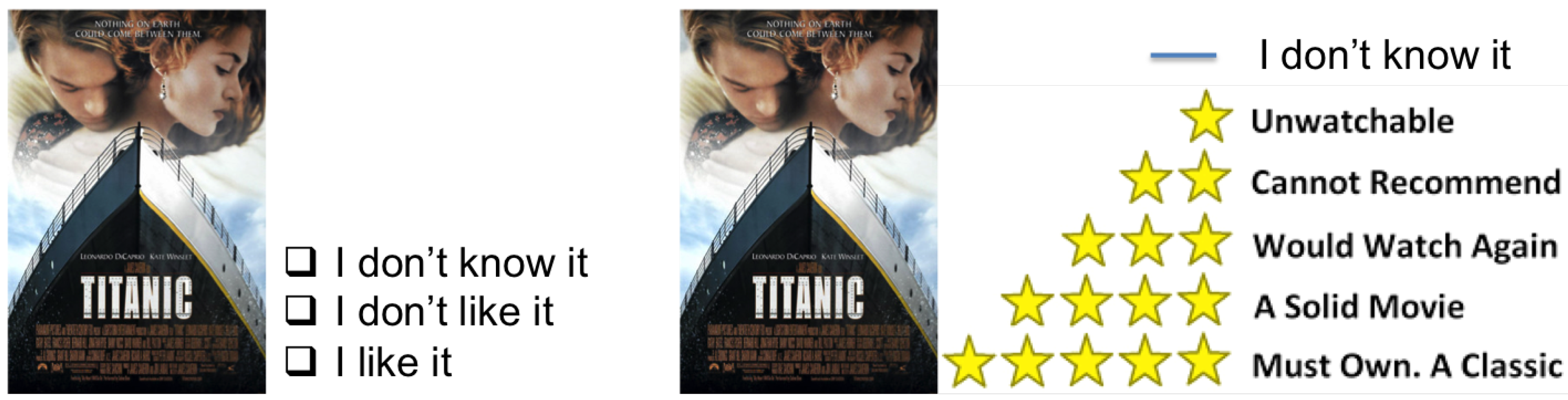
  • Active techniques interact with the new users in order to retrieve a small set of ratings that allows to learn the users’ preferences. A naive but extended approach is to question users about their interests and get their answers [9]. Such questions may include: ‘Do you like this movie?’, with possible answers such as: ‘Yes, I do’; ‘No, I do not’; ‘I have not seen it’. In fact, this process can be applied for cold-users in a sign-up process (a.k.a. Standard Interaction Model) or for warm-users (a.k.a. Conversational and Collaborative Model) where users can provided new preferences to the system; hence the system can better learn all users preferences [1].
In this paper, we focus on active learning to cope with the new user cold-start issue. Specifically, we study the collaborative filtering based techniques as they (1) have already demonstrated great accuracy for warm-users recommendations, (2) allow a fast generation of personalized recommendations to new users, and (3) only require users’ ratings. In fact, it has been demonstrated that few ratings from (new) users are more informative than using users’ attributes making it possible to obtain more accurate recommendations in cold-start situations [10]. As a consequence, we face a very challenging problem based on the advantages and drawbacks of the proposed techniques.
Active learning techniques propose a set of questions and answers to users in the form of a questionnaire. In our context, we refer to the questions as items and to the answers as the users’ preferences to these items. The questionnaires could be batch-oriented (several questions at once) or sequential (the questions are presented one after the other). In addition, the questions can be non-personalized (the same questions are asked to all users, e.g., most sold items), or personalized (the next questions depend on the users’ past answers). However, it was noted that users are not willing to answer many questions [1,2]. Therefore, the main challenge in active learning is to present short but very informative questionnaires with a maximum of 5–7 questions [4]). This maximizes the information retrieved from users and minimizes users’ efforts [11].
The personalization of the questionnaires led to a progressive understanding of the user’s preferences. In fact, the personalization of the questionnaires is close to a recommender system concept, although the latter seeks the items the user likes and the former seeks the items the user recognizes. In this context, we specifically focus on an optimization of the prediction accuracy, since it is directly linked to users’ satisfaction [1].
Current techniques for personalizing questionnaires in active learning collaborative filtering are based on decision trees. These techniques analyze the available warm-users’ ratings in order to find out which items to propose to users. However, their effectiveness in small datasets has not been probed. Moreover, we believe that taking into account warm-users’ predictions may enhance these techniques. In this paper, we suggest to exploit both available warm-users’ ratings and warm-users’ ratings predictions in order to improve the questionnaire. The experimentation shows that our approach enhances previously suggested ones in terms of accuracy and in using a smaller number of questions.
The remaining structure of this paper is organized as follows: Section 2 presents the state of the art for active learning using decision trees techniques. Section 3 gives the background and notation used for decision trees. Section 4 presents our contribution to enhance active learning based on past warm-users’ rating predictions. Section 5 shows the experimentations performed and the results of our approach. Finally we conclude and present our future works in Section 6.

2. Related Work in Active Learning

Active learning [12] is a data acquisition method that not only helps the system to learn cold users preferences, but also lets warm-users clarify and better express their preferences. Thus, the user is more self-conscious about his own preferences while the system continuously presents and discovers new items for the user. This represents a large exploration/exploitation challenge in recommender systems [6] and this will not be discussed further in this paper.
Active learning proposes to the (new) user to fill-out a questionnaire that will retrieve the first user’s preferences. The questions are simple and possible answers are limited. For instance a simple answers to the question ‘Do you like this movie?’ could be ‘Yes, I do like’; ‘No, I do not like’; ‘I have not seen it’. Furthermore, a ‘Rating Stars’ for the question ‘Can you rate this book?’ could be ‘I hate it (1 star)’; ‘I do not like it (2 stars)’; ‘It is acceptable (3 stars)’; ‘I like it (4 stars)’; ‘I love it (5 stars)’; ‘I have not read it’. Figure 1 represents a similar example.
As it can be noticed, the type of questions and answers represent a cost for the user. Therefore, there is a qualitative/quantitative trade-off in questionnaires: short number of questions and short number of answer’s choices lead into a quick filling of questionnaires, but the information retrieved could be not enough to understand new users’ preferences, whereas large questionnaires with multiple answer’s choices may challenge users’ willingness to fill (e.g., boring, too much rating debate, etc.). The personalization of the active learning aims to reduce the users’ effort and to maximize the system’s learning process for the effectiveness of the questionnaire [13].
In this research, we give a global related work of active learning, and we focus on active learning techniques in the domain of collaborative filtering recommendations, particularly those using decision trees as: (1) the sequential question paradigm allows a good personalization of the questionnaire [2], and (2) they aim to well profile a new user by asking as less questions as possible [4].

2.1. Personalization of Questionnaires and Strategies in Active Learning

The personalization of the questionnaire increases the information retrieved from users. Randomly selected candidate items (questions) are possibly not recognized by the new users. The static non personalized questionnaires show always the same candidate items regardless the user (e.g., most sold items), and hence the evolution of her tastes is not well captured. Personalized questionnaires alleviate these drawbacks. On the contrary, they may carry out a waiting time between questions [14], and the users are not willing to wait. Thus, the ideal questionnaire may intelligently present personalized candidate items and be fast to react to answers.
Active learning techniques have one or many strategies to pick up adequate candidate items. Some of them are given below and for a more detailed classification of these criterion strategies please refer to [2,9,12]:
  • Popularity, Variance and Coverage. Most popular items tend to have higher number of ratings, and thus they are more recognized. Popularity-based questionnaires increase the “ratability” [15] of candidate items in order to obtain a larger number of feedbacks, although very particular interests of new user preferences, out of popular items, are not captured. In addition, items with low rating variances are less informative. Thus, variance-based questionnaires show the uncertainty of the system about the prediction of an item [16]. In addition, the item’s coverage (i.e., number of users related to this item) can lead to creating interesting ratings’ correlation patterns between users.
  • Entropy. This strategy uses information theories, such as the Shannon’s Theory [17], to measure the dispersion of items ratings and hence to evaluate items informativeness. This technique tends to select rarely known items. In addition, entropy and popularity are correlated, and they are very influenced by the users’ ratability (capacity of users to know/rate the proposed items) [9].
  • Optimization. The system selects the items from those new feedbacks that may improve the prediction error rate, such as MAE or RMSE. Indeed, this is a very important aspect in recommender systems since error reduction is directly related to users’ satisfaction [1]. Other strategies may focus on the influence of queried item evaluations (influence based [18]), the user partitioning generated by these evaluations (user clustering [19], decision trees [20]) or simply analyze the impact of the given rating for future predictions (impact analysis [21]).
Three very well known non-personalized and batch-oriented strategies are: (1) Entropy0 relaxes the entropy constraints by supposing that unknown ratings are ratings equal to ‘0’ (changing a 1–5 rating scale to 0–5 rating scale), hence a high frequency of ‘0’ tends to decrease the entropy, (2) “LPE” (Logarithmic Popularity Entropy) chooses candidate items regarding their popularity and rating entropy [9], and (3) “HELF” (Harmonic Entropy Logarithmic Frequency) balances the entropy of candidate items against the frequency of rating repetitions [19]. However, the need of personalization in questionnaires has changed batch-oriented into sequential-oriented based questionnaires. This evolution is shown in [14,22,23,24,25]. In these papers, the authors have explained the importance of rapid online questionnaires and the ratability factor over candidate items in order to capture the users preferences. In the next section we focus on personalized questionnaires only.

2.2. Active Learning for Collaborative Filtering

The first appearance of active learning for new users cold-start was in [26], although the first step for creating sequential personalized questionnaires was suggested in [11]. In this paper, the authors enhance a similar approach in  [27] by assuming that users may not be able to rate presented items and thus relaxing the initial assumptions. They suggested a probabilistic collaborative filtering that uses bayesian networks to learn the candidate items entropy. The candidate items are presented sequentially and the whole model is re-adjusted according to past answers. However, these models do not perform well in on-line questionnaires because questions’ answers lead into a time-consuming model update. In [14] this idea was extended by questioning only the most popular items. This reduces the number of items to focus on and results in faster models. In [22] they applied active learning for matrix factorization. They argue that solving the new user cold-start is an optimization problem, which explores the latent space given by the matrix factorization to get new users parameters, then it exploits and adjusts these users parameters. Recomputing the whole matrix with each new rating is not tractable, and hence they propose a fast-online updating [28] after each answer.
One technique that is very meaningful in active learning is user partitioning. It allows to group users of similar tastes into clusters or nodes, and then tries to find out to which group the new user belongs to. In [19] the authors assumed that finding the correct users neighbors will improve the information gain of the questions presented to users. They presented the Information Gain through Clustered Neighbors (IGCN) algorithm to adjust the entropy of the items by taking into account only those users who match with the new user’s profile.
In [4] the authors use non supervised ternary decision trees to model the questionnaire. The decision trees are built off-line to be completely available for new users that receive the questions sequentially. To move to a new question they answer the current one by clicking on one of the three possible answers (‘like’, ‘hate’ and ‘unknown’). The users’ answers lead to a different child node of the ternary decision trees. This creates a personalized tree path that depends on the past users’ answers. On the other hand, this technique uses a collaborative filtering approach to build the decision trees. Using available users’ ratings, they seek the best discriminative item in order to split the population of users into three nodes (users who liked, those who hated and those who do not know this item). The best item is the one which minimizes a statistical error within the users’ ratings of the node. In order to evaluate the performance of the tree, the authors add labels to the candidate items by using the item average prediction method and demonstrated that their technique improves the accuracy of the system.
More recent research seems to focus on decision trees to handle questionnaires and on matrix factorization as a prediction model. The authors in [13] suggest to integrate decision trees construction into the matrix factorization model. They call it “Functional Matrix Factorization”. The first step is to learn about the underlying item feature vectors. In the second step, the users are defined as ratings’ vectors and one function maps these users into an underlying users features vector. This function is responsible for creating a ternary decision tree (‘like’, ‘dislike’, ‘unknown’). Hence, matrix factorization is applied to learn both function and items-features through an iterative alternating minimization process, which is performed in each node of the three. In [29], the authors claim that [13] is computationally too expensive. On the contrary, they suggested incorporating the matrix factorization into decision trees. They first build the decision tree as in [4]. Each node represents an item with an associated rating prediction label. The goal of the matrix factorization is to improve this label. Indeed, they train one matrix factorization model for each level of the tree, and aggregate users within the nodes into a pseudo-user for whom a prediction about the candidate item in the node is performed. This new predicted label replaces the last one.
Very recently, in [30] the authors assume that warm-users can be thought as new users from whom some ratings are known. Thus, this is seen as a supervised decision trees which internally reduces the accuracy of the technique by picking the best discriminative items. Moreover, they split the tree nodes into six, a 1–5 natural scale rating and an unknown node. This technique improves [4], and is later enhanced by (1) taking into account the most popular items only [14], and (2) using matrix factorization to improve the prediction labels assigned to the tree nodes [29].
The approaches in [4,30] use the big but not available Netflix dataset [31]. However, these approaches are not tested on smaller datasets, especially in terms of the number of users/ratings. In fact, a low number of users and ratings may produce an early pruning of some brunches of the tree. Moreover, early nodes with less data reduce the accuracy of the item’s average method and the discriminative items choice.

3. Background and Notation

The goal of decision trees in active learning is to split the users’ population in groups of users’ preferences. Thus, the users within the same tree’s node tend to share similar preferences. By going deeper inside the tree, these groups are refined and preferences are better detected. These techniques in a collaborative filtering context only have access to the available users/items feedback, i.e., ratings. As a consequence, they aim to find out the discriminative items that, in each node of the tree, efficiently split the users’ population depending on the users’ feedback to these items.
This idea is very useful to use with the new users’ cold start. One node is represented by one question about the discriminative item, e.g., ‘Do you like this item?’. The answers are the possible feedback of the new user to this item, e.g., ‘like’, ‘dislike’ and ‘unknown’. Every answer leads to a different question. Therefore, when new users fill-out the questionnaire, they are indeed following a personalized path which tries to detect to which group of users’ preferences they match the best.
In this paper, we will use the following notation for active learning using decision trees algorithms. Formally, let R be the available ratings. The rating of a user u in an item i is defined by r u , i R. In addition, let t be a node in the decision trees. We define U t , I t , and R t as the set of (warm) users, items and ratings currently in the node t. Furthermore, R t ( u ) and R t ( i ) are ratings of the user u and item i in the node t. In addition, our main contribution exploits the predictions over the existing R. Thus, we define P as the predicted set of R, so that for each r u , i R there is a prediction p u , i P. The set P is computed by using collaborative filtering techniques, e.g matrix factorization. Highlight that the number of users, items, and entries in R and P are the same. Particularly, we do not aim to predict sparse values or not known ratings from all possibles entry combinations of U t , I t . Finally, P t is the set of predictions currently in the node t, and P t ( u ) and P t ( i ) are the set of users and items predictions in the node t. Table 1 resumes these notations.

4. Active Learning Decision Trees

This section introduces our contribution. We suggest exploiting not only the available ratings from “warm” users, but also the predictions made by collaborative filtering algorithms over these available ratings. We first give some considerations to decision trees for small datasets as long as the current state of the art has not been tested in these environments. Second, we illustrate our core idea using a real use-case for a better discussion and understanding. We use two datasets from MovieLens  (http://grouplens.org/datasets/movielens/). Besides, we show the properties of the Netflix dataset [31] for datasets’ size comparisons. These datasets are later used in Section 5 to evaluate our approach and their properties are given in Table 2. Third, we present the techniques and algorithms for decision trees in non supervised and supervised techniques. In addition, a complexity analysis of our algorithms is provided.

4.1. Decision Trees in Small Datasets

The active learning in collaborative filtering is more challenging in small datasets since there is less data to make correlations with. Particularly, we discuss the concentration of ratings and users in the nodes of the tree in three co-related aspects: (1) the number of child nodes in a tree, (2) the number of ratings in a node, and (3) the number of users in a node. We do not strictly address this, although as it will be shown in the experimentation phase, we improve the current approaches under this context as well.
The number of child nodes in which the current node t is split plays an important role in small datasets. In big datasets, using a large scale of answers may yield better accuracy while classifying users’ preferences. The large number of users in the dataset is split among all child nodes. Moreover, the less informative node, the group for ‘unknown’ is always the most populated due to the sparse nature of datasets [4]. As a consequence, the tree child nodes containing small number of users tend to be pruned faster. In addition, less populated nodes may result in an unstable performance since there is not much data to correlate. In datasets with less number of users we suggest using short scale answers, such as ‘like’, ‘dislike’ and ‘unknown’. This allows to aggregate users into the same node to ensure the usefulness of the tree.
Moreover, the number of ratings in a tree node helps the system to analyse current items, to find out the best discriminative items and to assign a prediction label to them. This factor is used in [4] as a stopping criteria. The authors claim that there is a very little gain in going further in analyzing nodes with few ratings. Nevertheless, we consider that the number of users should be taken into considerations as well. The number of ratings in a node is directly related to the number of users in this node. This is important in the field of recommender systems since users’ preferences with higher number of ratings are better detected. On the contrary, having less number of ratings per user may lead to a bad understanding of users’ preferences. In decision trees, nodes containing few users but many ratings perform better in preference detection than nodes containing many users with fewer ratings. As a result, taking into account ratings only may yield to unstable performances in small datasets.

4.2. Warm-Users Predictions in Decision Trees

Users are not willing to rate too many items. Hence, the main challenge of active learning is to learn the (new) users’ preferences as soon as possible by creating a short but informative questionnaire. In this section we explain the core of our contribution which is to use the prediction of available ratings to enhance active learning using decision trees.
Current decision trees techniques exploit only the available ratings in R in order to (1) find the discriminative items, (2) split the users’ population, and (3) compute predictions over the candidate items. For instance, let us fix the decision trees analysis into the node t. These techniques iterate among items in I t and analyze their impact in R t . This impact is typically measured by associating an error when splitting users using their preferences to these candidate items. The goal is to find out, for each node of the tree, the best discriminative item that optimizes this error.
In addition, these techniques use a simple item prediction method based on the “item rating average” in order to evaluate a prediction accuracy and to compute prediction labels for candidate items. Note that this technique is adequate for large datasets, which allows a quick and acceptable generation of predictions from the available ratings in R t . furthermore, using more accurate prediction techniques is possible but (1) it is very expensive and time consuming to do it for every node of the tree, and (2) the predictions needed in decision trees are item-oriented regardless of the user (the same item prediction value to any user) rather than user-item oriented (items’ predictions depend on users’ interests).
We propose to change this paradigm by using more accurate predictions over the available ratings R. The main idea is to introduce the prediction P as a new source of useful data. Hence, R and P are available from the root node of the tree. Then, when the node is split into child nodes, R t is split into R t c h i l d . As long as we want to preserve that for every rating r u , i R t there is an associated prediction p u , i P t , for every node t we split P t into P t c h i l d as well. This idea is illustrated in Figure 2. In addition, we propose to use the available ratings in R only to split the users population, and P to find out the best discriminative items to enhance the prediction label of candidate items.
This makes sense since finding discriminative items and label predictions are associated with computing an error. As long as P is built by using more accurate methods than the “item rating average”, this error is minimized efficiently. We propose using efficient algorithms, such as matrix factorization [32]. The main drawback of using matrix factorization is that it computes different item predictions for different users. The decision trees require a unique item prediction value to be applied to any user. In [4,30] the authors use the “item rating average” within R t . We suggest using a similar method, with a major difference that is computing the “item prediction average”, which is indeed the average of the predictions within P t .
Collaborative filtering methods are very accurate for recommending items to users by replicating the users’ rating behavior. As a consequence, they are good as well in guessing the average prediction of users, items, and in general the average rating value of the dataset. We illustrate this by using a real use-case. We perform the matrix factorization (MF) predictions over the Movielens 1M dataset in Table 2 to obtain the predicted values P for R. Table 3 summarizes statistics over R and P. One can see how close the statistic values such as the mean and quartiles between the available ratings and the predicted ratings are.
In addition, we want to go further by considering different users’ populations. We compare the performance of three different predictors: (1) the item rating average (Item-Avg), (2) the matrix factorization (MF), and (3) the matrix factorization average (MF-Avg). The first sets the item’s rating average as the item’s prediction. The second decomposes a matrix R into two random matrices in such a way that the multiplication of both matrices gives approximately the original R [32]. The third uses a matrix of predictions over available ratings given by the matrix factorization to set the item’s prediction average as the item’s prediction. Our goal is to show that (1) as demonstrated, the matrix factorization performs better in terms of accuracy than the item rating average method, and (2) the item prediction average predictions are close to the item rating average predictions.
This analysis is performed as follows. First, we obtain P by performing the matrix factorization over the available R. Second, we count the number of ratings per user and we divide the users into groups; users having less than 50 ratings, less than 100 ratings, etc. highlight that these groups are incremental and thus one user may belong to more than one group. For each of these groups, the users’ ratings and the corresponding users’ predictions are taken from R and P into separated sets R and  P . Third, we evaluate the performance of predictions in P by computing the root mean square error (RMSE). Moreover, we perform the item rating average over R , and item prediction average (MF-Avg) over P , in order to observe their performance as well. The results are given in Figure 3a,b. As expected, MF outperforms the item rating average method. In addition, we observed that MF-Avg attempts to imitate the behavior of the item rating average method. Hence, the item prediction average is also an acceptable predictor regarding the item rating average. In fact, one can observe that item rating average and item prediction average are closer while dealing with more users and ratings. This behavior is perfect in decision trees since the top of the tree is more populated by users and ratings. On they contrary, they diverge while dealing with less users and ratings. This means the accuracy in larger decision trees will decrease. As long as active learning aims to create short questionnaires, this will not a great impact on our approach.

4.3. The Decision Trees Algorithms

This section presents the algorithms used to develop our approaches for decision trees. We can apply our contribution to non supervised and supervised decision trees techniques. Their main drawback is the heavy analysis needed to find out the best discriminative item. For instance, given the current node t, these techniques iterate over all candidate items i I t by analyzing users’ ratings on i. The population of users are then grouped into users’ who rated item i and users who did not. Typically, the latter is more populated due to the sparse nature of the available dataset. Furthermore, the users who rated item i can be grouped into further categorizations, e.g., users who liked/hated, or who rated ‘1, 2, 3, 4, 5’. Then, the population of users in these nodes, and their ratings, are used to evaluate the performance of choosing i as one discriminative item of R t .
The difference between supervised and non-supervised approaches is that the former assumes that “warm”-users can be considered as “cold”-users from which some ratings are known, and hence, the known users’ ratings can be used to validate the technique. As a consequence, it is possible to compute an error based on the prediction accuracy, such as RMSE. On the contrary, since non supervised techniques do not have any validation, they compute a statistical error based on the available ratings in the node. Nevertheless, in both approaches a validation is not possible in the ‘unknown’ nodes, since by definition, there is no rating label for these users to this item. As a consequence, the statistical error is mandatory in this case. Our approach uses similar statistics as [4].

4.3.1. Non Supervised Decision Trees for Active Learning

In [4], the authors define a set of statistics and an internal error using these statistics to find out the best discriminative item. In this approach, the best item is the one which reduces this error. In addition, as long as the tree nodes contain many ratings, they use the item rating average method to compute item label predictions for items.
We suggest to use the predictions P over the available ratings in R in order to enhance this technique. Formally, given the node t, there are ratings r u , i R t so that u U t and i I t . In addition, for each rating r u , i there is an associated prediction p u , i P t . The goal is to find out, among all candidate items j I t , the best discriminative item i . To do that, we compare the current state of the node t to the impact of picking j as discriminative item, as explained below.
The current status of the node j is given by all the items’ ratings in P t . The properties of this status are given by the statistics presented in Equation (1), which consider separately all items in the node. These statistics are simple aggregations over ratings on node j and they allow to glimpse a current state error as Equation (2), which is indeed the error contribution of every item j in the node t.
j I i : s u m ( t ) j = u U t P ( j ) p u , j s u m 2 ( t ) j = u U t P ( j ) p u , j 2 n ( t ) j = | u U t P ( j ) |
e 2 ( t ) = j s u m 2 ( t ) j ( s u m ( t ) j ) 2 / n ( t ) j
We then look for the best candidate item that minimizes this current error. Thus, we analyze the impact of every item j within this node t and the child nodes. We first suppose that j is a discriminative item and we split U t into 3 childs: t L for users who liked j ( r u , j ≥ 4), t D for users who did not like ( r u , j ≤ 4)) and t U for users who do not know the item (absence of rating). Highlight that we use R t to split the users’ population. In addition, we delete the presence of discriminative item ratings in child nodes. As a consequence, one has 3 rating subsets R t L , R t D and R t U in child nodes U t L , U t D and U t U , respectively. The impact of picking j as candidate item is given by the error of these three nodes: E r r t ( j ) = e 2 ( t L ) + e 2 ( t D ) + e 2 ( t U ) . This means that one evaluates the status of the given child nodes by using the Equation (2) and associated subsets P t L , P t D and P t U . However, the number of users in the unknown node t U is normally much larger than in other groups, and hence, the computation is heavier in this node. To avoid this, it is possible to deduce statistics for t U from the node t and the other child nodes t L and t D , as represented in Equation (3):  
s u m ( t u ) j = s u m ( t ) j s u m ( t L ) j s u m ( t D ) j s u m 2 ( t u ) j = s u m 2 ( t ) j s u m 2 ( t L ) j s u m 2 ( t D ) j n ( t u ) j = n ( t ) j n ( t L ) j n ( t D ) j
By doing this analysis with every candidate item j I t , one obtains an associated impact E r r t ( j ) . The discriminative item is the one which minimizes such error, i = a r g m i n E r r t ( j ) , and then it is used as the real splitter to continue the construction of the tree in lower levels.
Finally, once the discriminative item is chosen, the prediction label associated to the tree is given by the item prediction average, i.e., average value of P t ( i ) .
This approach is similar to [4], with two major differences. First, the available ratings are only used to split the population of users. As a consequence, the statistics and the items predictions are computed by using the proposed set of predictions P. Second, once a discriminative item is chosen in a parent node it does not pass to the child nodes. This is done for two reasons: (1) to avoid choosing the same item, and hence, to avoid to pose twice the same question to the same user, and (2) to delete the influence of the items’ ratings in the child nodes. In fact, one can avoid choosing an item without deleting their ratings as done in [4]. Algorithm 1 shows this approach.
Algorithm 1 Non-supervised decision tree algorithm
 1:functionBuildDecisionTree( R t , P t , currentTreeLevel)
 2:    for rating r u , i in R t do
 3:        accumulate statistics for i in node t using p u , i
 4:    end for
 5:    for candidate item j in I t do
 6:        for r u , j in R t ( j ) do
 7:           obtain P t ( u )
 8:           split U t into 3 child nodes based on j
 9:           find the child node where u has moved into
10:           for rating p u , i in P t ( u ) do
11:               accumulate statistics for i in node t c h i l d using p u , i
12:           end for
13:        end for
14:        derive statistics for j in node t U from the t L and t D statistics
15:        candidate error: e t ( j ) = e t L ( j ) + e t D ( j ) + e t U ( j )
16:    end for
17:    discriminative item i = a r g m i n i e t ( i )
18:    compute p i by using item prediction average
19:    if currentTreeLevel < maxTreeLevel then
20:        create 3 child nodes U t c h i l d based on i ratings
21:        for child in child nodes do
22:           exclude i from R t c h i l d
23:           BuildDecisionTree( R t c h i l d , P t c h i l d , currentTreeLevel +1)
24:        end for
25:    end if
26:    return i
27:end function

4.3.2. Supervised Decision Trees for Active Learning

In [30], the authors suggested using warm-users as cold-users from whom some interests are known. This assumption allows to create a supervised decision trees where some labels are known for validation purposes.
We again suggest to use the predictions P over the available ratings in R in order to enhance this technique. Given the current node t, there are warm-users in U t who have ratings in R t and predictions in P t . This technique considers warm-users as cold-users from who some ratings are known. Thus, we split the users ratings into training ratings R t t r a i n and validation ratings R t v a l i d a t i o n . The former represents the interests of the warm-users. The latter are the items labels given when considered as cold-users. Note that we consider the perfect case where a user u and and item j and in U t t r a i n , U t v a l i d a t i o n and I t t r a i n , I t v a l i d a t i o n respectively. As long as for each rating r u , i there is an associated prediction p u , i P t , it is possible to obtain P t t r a i n as well.
As a result, the current node t contains ratings in R t t r a i n , predictions in P t t r a i n , and ratings for validation purposes in R t v a l i d a t i o n . The goal is to find out, among all candidate items j I t , the best discriminative item i . To do that, we compare the current state of the node t to the impact of picking j as discriminative item as explained below.
On the one hand, the state of the node t is given by the Root Mean Square Error (RMSE), which computes the squared difference between current predictions and real observed ratings. Predictions are computed by using the “item predicion average” method over P t t r a i n . Observed ratings are taken from R t v a l i d a t i o n . Therefore, each user u U t is associated to one error R M S E 1 u . The current error in the node is the sum of all user’s errors. On the other hand, we look for the best candidate item that minimizes this current error. Thus, we analyze the impact of every item j within this node t and the child nodes. We first suppose that j is a discriminative item and we split U t into 3 childs: t L for users who liked j ( r u , j ≥ 4), t D for users who did not like ( r u , j ≤ 4)) and t U for users who do not know the item (absence of rating). Highlight that we use R t t r a i n to split the users’ population. In addition, we delete the presence of discriminative item ratings in child nodes. As a consequence, one has 3 rating subsets R t t r a i n L , R t t r a i n D and R t t r a i n U in child nodes U t t r a i n L , U t t r a i n D and U t t r a i n U , respectively. Hence, it is possible to compute the state of the child nodes as it was performed before. This creates a second user error, R M S E 2 u . The impact of picking j as candidate item for the user u is Δ u , i = R M S E 1 u R M S E 2 u . Thus the impact of picking j as candidate item for the node t is given by the sum aggregation of all impacts of j.
The number of candidate items to analyze can be very large. We take into account only the 200 most popular items, as done in [30]. This yields in very acceptable accuracy and a great reduction in the time analysis.
Therefore, after the analysis of all users and candidate items, the item in R t t r a i n associated to a higher overall impact is picked as discriminative item i , since the maximum value here means a higher error difference. Finally, the predicted label for this discriminative items is given by the item prediction average over current node P t .
This approach is similar to [30], with two major differences: (1) P is used to validate the approach, and to obtain items label for the chosen discriminative items, and (2) we split the nodes into 3 child nodes (’like’, ’dislike’, ’unknown’) rather than 6. This warrants a minimum number of users in child nodes to avoid fast pruning in small datasets. Algorithm 2 shows this approach.
Algorithm 2 Supervised decision tree algorithm
 1:functionBuildDecisionTree( U t , R t t r a i n , R t v a l i d a t i o n , P t , currentTreeLevel)
 2:    for user u U t do
 3:        compute R M S E u 1 on R t v a l i d a t i o n ( u ) and P t ( u )
 4:    end for
 5:    for candidate item j from R t t r a i n do
 6:        split U t into 3 child nodes based on j
 7:        for user u U t do
 8:           find the child node where u has moved into
 9:           compute R M S E u 2 on R t v a l i d a t i o n ( u ) and P t ( u )
10:            Δ u , i = R M S E u 1 R M S E u 2
11:        end for
12:    end for
13:     δ = aggregate all Δ u , i
14:    discriminative item i = a r g m a x i δ i
15:    compute p i by using item prediction average
16:    if currentTreeLevel < maxTreeLevel and Δ i 0 then
17:        create 3 child nodes U t c h i l d based on based on i ratings
18:        for child in child nodes do
19:           exclude i from R t c h i l d
20:           BuildDecisionTree( U t c h i l d , R t c h i l d t r a i n , R t c h i l d v a l i d a t i o n , P t c h i l d , currentTreeLevel+1)
21:        end for
22:    end if
23:    return i
24:end function

4.4. Complexity of the Algorithm and Time Analysis

The complexity of our approaches for non-supervised decision trees and supervised decision trees is very similar to [4,30]. In fact, despite some differences in the way of computing the error that needs to be improved, these algorithms follow a similar procedure. The complexity of splitting the users in node t is O ( u U t | R t ( u ) | 2 ) , and thus, for all the nodes in the same level we use O ( u U | R ( u ) | 2 ) . As a consequence, the complexity to build a tree of N questions is O ( N u U | R ( u ) | 2 ) . In fact, adding the prediction set P does not affect the complexity of the algorithms, although, it does affect the memory footprint of the approaches. Considering that ratings R and predictions P sets are coded equally, our approach consumes double of the memory size to store the set P. In addition, extra runtime is required to split both R and P accordingly.
The time-consumption of the algorithms is similar as well. A little extra time is needed in our approaches in order to deal with the split of the prediction in P. In addition, in comparison to [30] our supervised approach is faster due to the reduced number of child nodes.

5. Experimentation

The goal of our experimentation is two-fold (i) to present the behaviour of current techniques in smaller datasets and (ii) to show the performance of our presented approach. Recent techniques have presented their results using Netflix dataset. However, this dataset is no longer available for research. Hence, we use two versions of the Movielens dataset. Table 2 describes the properties of these datasets.
Since our approach considers external prediction techniques as a new source, in order to build our decision trees we use matrix factorization [32] due to its accuracy. We compare our approach in non supervised decision trees, as in [4], and in supervised decision trees, as in [30].
The technique in [4], denoted “Golband”, uses two parameters: bias overfitting λ 1 and rating overfitting λ 2 . We set empirically these parameters to λ 1 = 7 and λ 2 = 200 . The technique in [30], denoted “Karimi”, uses a rating overfitting parameter λ 2 . Our approaches are identified as “Pozo Non Supervised” and “Pozo Supervised”, and they do not contain any parameters, which represents an advantage in comparison to the state of the art.
As long as non supervised decision trees and supervised decision trees require different settings, we explain these experimentations separately. In order to compare the approaches we use the RMSE metric oriented to users, which measures the squared difference between the real ratings and the predicted ratings:
R M S E u = 1 N ( r u , i p i ) 2
where N is the number of ratings of the user u, p i is the predicted label value of the candidate item in the question node and r u , i is the real rating of the user u for the item i. Hence, the evaluation of the error in one question is the average of the users error in this question number. As a consequence, for this metric the lower is the better.
Knowing that the experimentation may depend on the split of the dataset, we run it 50 times and then used the mean value of the RMSE. We use this process to evaluate the performance for the MovieLens 1M and MovieLens 10M.

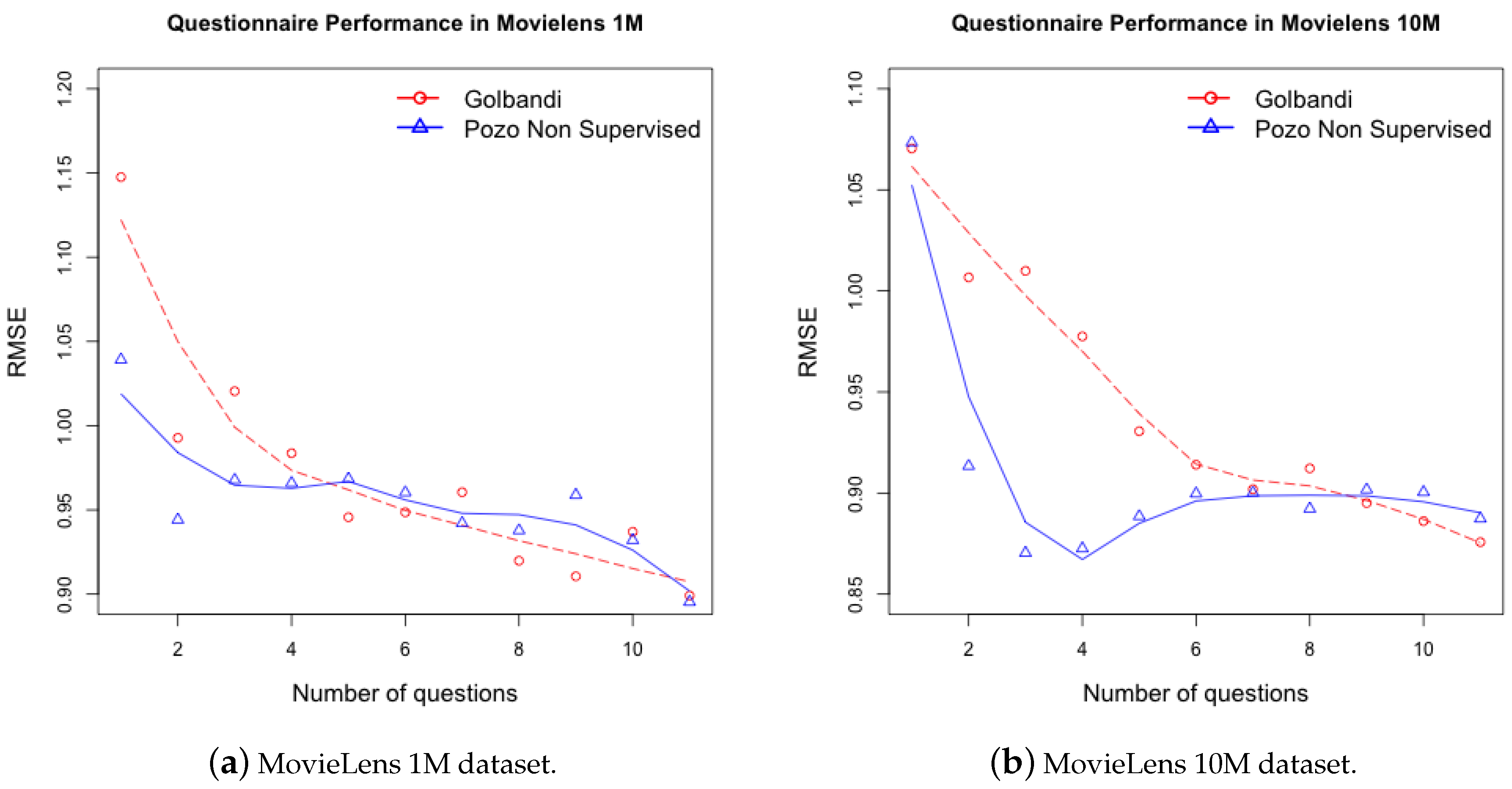
5.1. Non Supervised Decision Trees

The experimentation carried out in [4] splits the datasets into 90% training set, D t r a i n and 10% test set, D t e s t . However, this is not a real cold-start context since the same user may appear in both training and test set. We suggest a real cold-start situation. We split the set of users in the datasets into 90% training set, U t r a i n and 10% test set, U t e s t . Hence, the users in the training set help to build the decision trees and the users in the test set are considered as new user to evaluate the performance of the approach.
The process we have followed to run this experimentation is as follows. First we split the dataset into U t r a i n and U t e s t . Second, we compute the collaborative filtering algorithms over ratings R in U t r a i n and we extract the associated predictions P. Third, we train the approach of “Golbandi" by using U t r a i n . Our approach is trained by using both ratings in training set R and the prediction of the training set P. Finally, the performance of the decision trees is evaluated by using the test set U t e s t . The users in this set are used to answer the questions. If the item is known, we compute the RMSE associated to this answer and this question. Then, the user answers a new question. At the end, we compute the average of the accumulated nodes RMSE.
Figure 4a,b show the results (the mean point values and tendency curves) of this experimentation for MovieLens 1M dataset and MovieLens 10M dataset respectively.
Our approach achieves a lower error with less number of questions. This matches with the needs of active learning; short but very informative questionnaires. This is possible due to the higher accuracy of the matrix factorization. In addition, we notice that the approaches tend to an asymptotic behavior in both Movielens datasets. This corresponds to a case in which users are very profiled, and further knowledge is complicate to extract.
Furthermore, it is interesting to comment the particularity in Figure 4b. “Golbandi” slowly decreases the error and starts finding the asymptote behavior at question 11. Our approach gives very informative questions at the beginning, making the error to decrease very fast. Further than question 4, our approach proposes less informative questions and thus the error slightly increases between the questions 6 and 8. The algorithm is looking for new more informative questions than before, what makes the error decreases again from question 9, and to slowly meet the asymptote.

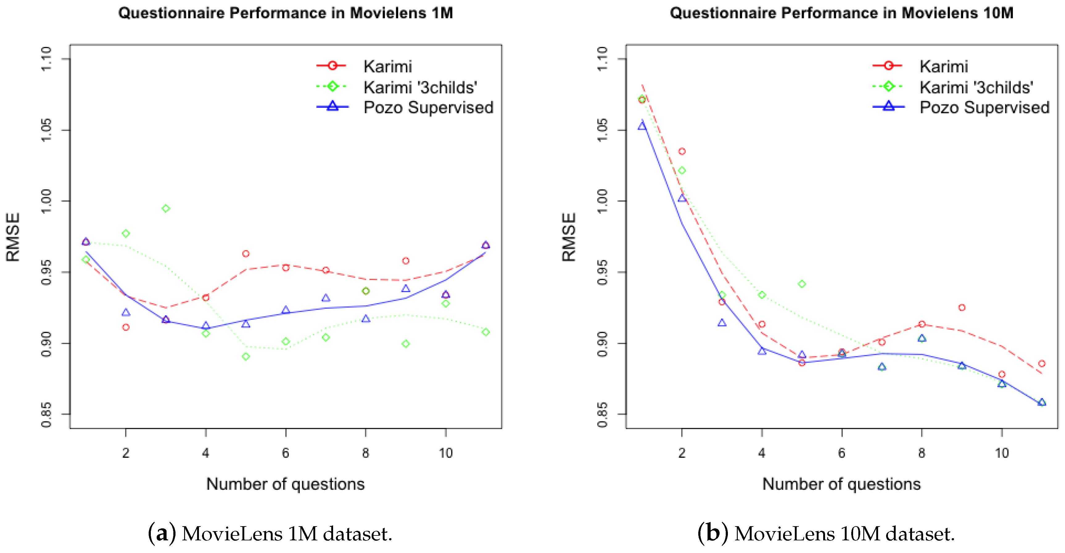
5.2. Supervised Decision Trees

The experimentation carried out in [30] use a four-fold set to evaluate their dataset. The Netflix dataset is already split into 90% training set, D t r a i n , 10% test set, D t e s t . In order to evaluate their technique in cold-start situations, they merge both sets and split the result into 75% user training set, U t r a i n and 25% user test set U t e s t , where users in one set are not present in the other. Then, they cross these 4 sets to create their own settings environment. To train the decision trees they intersect D t r a i n and U t r a i n to get a training set R t r a i n . They use the intersection of D t e s t and U t r a i n to obtain the validation set R v a l i d a t i o n . To evaluate the technique, they use the intersection of D t r a i n and U t e s t as the answer set R a n s w e r , whereas the intersection of D t e s t and U t e s t is the performance set R p e r f o r m a n c e used to evaluate the RMSE performance of the technique.
“Karimi” chose these experimentation settings in order to publish and compare results using the pre-defined D t r a i n and D t e s t Netflix dataset. In addition, we consider that picking up 25% of users the for test set, U t e s t is concerned with the posteriori search of R a n s w e r and R p e r f o r m a n c e . The more users in the test set the more probability to pick up ratings from D t r a i n and D t e s t for R a n s w e r and R p e r f o r m a n c e , respectively. Thus, more test points are possible possible to use.
We simplify the setting above. The process we have followed in the Movielens datasets is as follows. We split the dataset into 90% user training set, U t r a i n and 10% user test set U t e s t , where users in one set are not present in the other. Then, the ratings in U t r a i n are split into 90% rating training set, R t r a i n , and 10% ratings validation set R v a l i d a t i o n . The U t e s t is not split into “answer” and “performance” and it is completely used for probing the approach.
We train “Karimi” by using these settings. In addition, we train a modification of “Karimi” to take into account only 3 child nodes, denoted “Karimi 3 childs”. Figure 5a,b show the results (the mean values and tendency curves) of this experimentation for both MovieLens datasets.
On the one hand, one may observe that our approach achieves a lower error (around 1%) in less number of questions; hence we better capture the preferences of new users. Therefore, our approach still matches with the needs of active learning: short but very informative questionnaires. This is possible due to the higher accuracy of the matrix factorization based predictions. In addition, it is expected to have an asymptotic behavior in large number of questions for both Movielens datasets.
On the other hand, we highlight the non-stability of “Karimi” in Figure 5a. Karimi splits parent nodes into 6 child nodes per level; hence the Movielens 1M dataset has not enough users and ratings in deeper nodes of the tree, and thus it causes this dysfunction. The Karimi “3 childs” implementation enhances this issue by aggregating users into 3 child nodes (“like”, “dislike” and “unknown”). However, our approach overcomes both approaches above. Highlight that the Karimi modification and our approach show close results. In fact, the difference is too small to be perceived in Figure 5b. In addition, one may observe an increase of the error after 6 questions due to the smaller number of users and, again, the fast previously found informative questions.

5.3. Time Analysis

We conclude the experimentations by comparing the time analysis within the different approaches. We use a virtual machine in the cloud with 6 cores Intel(R) Xeon(R) CPU E5-2650 at 2.00 GHz and 14 Gb RAM. The techniques are implemented using a Java multi-threading approach, which distributes the analysis inside the tree nodes. Our non supervised approach increases the time consumption of Golbandi by around 1%, which might be considered as insignificant. On the contrary, the supervised approach reduces the time consumtion of Karimi by around 50% due to the reduced number of child taken into consideration.

6. Conclusions

Recommender Systems suffer from new user cold-starts. This issue is more acute in collaborative filtering techniques since they only rely on users’ ratings to generate recommendations. In order to learn the (new) users’ preferences, passive recommender systems wait for sporadic ratings from users. On the contrary, active learning is proposed as a data acquisition method that gathers users’ ratings by presenting a simple questionnaire to users. For instance, ‘Do you like this item?’: ‘Yes, I do like’; ‘No, I do not like’; ‘I have not seen it’. However, users are not willing to answer many questions or to rate many items. Therefore, the main goal of active learning is to create a short but efficient and informative questionnaire.
The state of the art has evolved from non personalized batch-oriented techniques (giving many questions at once and the same questions to any user) to personalized sequential-oriented questionnaires (giving questions one by one taking into account the past current users’ answers). In our point of view, the personalization of the active learning technique is crucial to better learn the new users preferences and current methods based on decision trees are interesting techniques to model questionnaires. Indeed, the personalization of decision trees allows to predict with which items the new user has been in contact, and present them to the users.
However, active learning techniques based on decision trees have not been applied to small datasets. A lower number of users and ratings affect the performance of these algorithms. In addition, we consider that recent approaches do not properly consider the prediction of candidate items. On the one hand, they use very simple prediction methods to make the decision trees tractable. On the other hand, they only exploit the users’ ratings.
In this paper we proposed using two sources in the decision trees active learning technique. The main idea is to train an accurate collaborative filtering techniques with a ratings dataset to generate a prediction dataset. Both ratings and predictions dataset are used inside the decision trees. The former properly split the users’ population while building the tree. The latter enhances the seek of the best discriminative items (questions) and better predict the associated labels. We have tested this approach in non supervised decision trees and supervised decision trees techniques.
The experimentation uses two publicly available datasets: Movielens 1 million ratings and Movielens 10 million ratings. We show that our approach enhances the state of the art in terms of RMSE and the related number of questions. In fact, we find better questions and better predictions that make it quicker reduce the error. This is especially useful in small dataset contexts, where the low number of users and ratings do not allow to create big decision trees.
Finally, the approach suggested in this paper allows to alleviate the new user cold start, issue that, together with the scalability and large items/users representations, is a big challenge in the domain of recommender systems.
As a perspective and future work, we consider that there are other resources that appear in questionnaires and may be very useful and informative in collaborative filtering active learning techniques. We especially believe that the study of users behavior as in [33,34] and also the time (new) users spent to answer a question are very significant for extracting the users’ preferences. Thus, we focus on “time-aware” recommendation techniques and decision trees to retrieve and exploit not only the users’ answers but also the users’ behavior. On the one hand, we will study new Slope-One [35] techniques to create time-aware off-line questionnaires due to their scalability and reactivity. On the other hand, other collaborative filtering techniques have already demonstrated their compatibility with timestamped preferences [36]. However, time-aware techniques tend to be timely expensive whereas active learning techniques require of fast adaptability to the current users’ answers. As a result, the challenge is to create accurate, scalable recommendation models that evolve in real-time to cope with cold-start issues.

Author Contributions

All authors have contributed equitably to the implementation of the approaches presented in this paper. The work was done jointly in the laboratories in Paris and Manchester. The algorithms have been implemented by M.P. and have been tested and validated by R.C. The experimental phase was under the responsibility of F.M. and E.M.

Funding

This work has been supported by “FIORA” project, and funded by “DGCIS” and Conseil Regional de l’Ile de France.

Conflicts of Interest

Declare conflicts of interest or state “The authors declare no conflict of interest”. Authors must identify and declare any personal circumstances or interest that may be perceived as inappropriately influencing the representation or interpretation of reported research results. Any role of the funding sponsors in the design of the study; in the collection, analyses or interpretation of data; in the writing of the manuscript, or in the decision to publish the results must be declared in this section. If there is no role, please state “The founding sponsors had no role in the design of the study; in the collection, analyses, or interpretation of data; in the writing of the manuscript, and in the decision to publish the results”.

References

  1. Rubens, N.; Elahi, M.; Sugiyama, M.; Kaplan, D. Active learning in recommender systems. In Recommender Systems Handbook; Springer: Berlin, Germany, 2015; pp. 809–846. [Google Scholar]
  2. Elahi, M.; Ricci, F.; Rubens, N. Active Learning in Collaborative Filtering Recommender Systems. In E-Commerce and Web Technologies; Springer: Berlin, Germany, 2014; pp. 113–124. [Google Scholar]
  3. Su, X.; Khoshgoftaar, T.M. A survey of collaborative filtering techniques. Adv. Artif. Intell. 2009, 2009, 421425. [Google Scholar] [CrossRef]
  4. Golbandi, N.; Koren, Y.; Lempel, R. Adaptive bootstrapping of recommender systems using decision trees. In Proceedings of the Fourth ACM International Conference on Web Search and Data Mining, Hong Kong, China, 9–12 February 2011; pp. 595–604. [Google Scholar]
  5. Karimi, R.; Freudenthaler, C.; Nanopoulos, A.; Schmidt-Thieme, L. Comparing prediction models for active learning in recommender systems. In Proceedings of the LWA 2015 Workshops: KDML, FGWM, IR, and FGDB, Trier, Germany, 7–9 October 2015. [Google Scholar]
  6. Kantor, P.B.; Ricci, F.; Rokach, L.; Shapira, B. Recommender Systems Handbook; Springer: Berlin, Germany, 2011; p. 848. [Google Scholar]
  7. Peis, E.; del Castillo, J.M.; Delgado-López, J. Semantic recommender systems. Analysis of the state of the topic. Hipertext. Net 2008, 6, 1–5. [Google Scholar]
  8. Karim, J. Hybrid system for personalized recommendations. In Proceedings of the International Conference on Research Challenges in Information Science (RCIS), Marrakesh, Morocco, 28–30 May 2014; pp. 1–6. [Google Scholar]
  9. Rashid, A.M.; Albert, I.; Cosley, D.; Lam, S.K.; McNee, S.M.; Konstan, J.A.; Riedl, J. Getting to know you: Learning new user preferences in recommender systems. In Proceedings of the 7th International Conference on Intelligent User Interfaces, San Francisco, CA, USA, 13–16 January 2002; pp. 127–134. [Google Scholar]
  10. Pilászy, I.; Tikk, D. Recommending new movies: even a few ratings are more valuable than metadata. In Proceedings of the Third ACM Conference on Recommender Systems, New York, NY, USA, 22–25 October 2009; pp. 93–100. [Google Scholar]
  11. Harpale, A.S.; Yang, Y. Personalized active learning for collaborative filtering. In Proceedings of the 31st Annual International ACM SIGIR Conference on Research and Development in Information Retrieval, Singapore, 20–24 July 2008; pp. 91–98. [Google Scholar]
  12. Chaaya, G.; Metais, E.; Abdo, J.B.; Chiky, R.; Demerjian, J.; Barbar, K. Evaluating Non-personalized Single-Heuristic Active Learning Strategies for Collaborative Filtering Recommender Systems. In Proceedings of the 2017 16th IEEE International Conference on Machine Learning and Applications (ICMLA), Cancun, Mexico, 18–21 December 2017; pp. 593–600. [Google Scholar] [CrossRef]
  13. Zhou, K.; Yang, S.H.; Zha, H. Functional matrix factorizations for cold-start recommendation. In Proceedings of the 34th International ACM SIGIR Conference on Research and Development in Information Retrieval, Beijing, China, 25–29 July 2011; pp. 315–324. [Google Scholar]
  14. Karimi, R.; Freudenthaler, C.; Nanopoulos, A.; Schmidt-Thieme, L. Active learning for aspect model in recommender systems. In Proceedings of the Symposium on Computational Intelligence and Data Mining (CIDM), Paris, France, 11–15 April 2011; pp. 162–167. [Google Scholar]
  15. Carenini, G.; Smith, J.; Poole, D. Towards more conversational and collaborative recommender systems. In Proceedings of the 8th International Conference on Intelligent User Interfaces, Miami Beach, FL, USA, 12–15 January 2003; pp. 12–18. [Google Scholar]
  16. Boutilier, C.; Zemel, R.S.; Marlin, B. Active collaborative filtering. In Proceedings of the Nineteenth Conference on Uncertainty in Artificial Intelligence, Acapulco, Mexico, 7–11 August 2003; Morgan Kaufmann Publishers Inc.: Burlington, MA, USA, 2002; pp. 98–106. [Google Scholar]
  17. Shannon, C.E. A mathematical theory of communication. ACM Sigm. Mob. Comput. Commun. Rev. 2001, 5, 3–55. [Google Scholar] [CrossRef]
  18. Rubens, N.; Sugiyama, M. Influence-based collaborative active learning. In Proceedings of the 2007 ACM Conference on Recommender Systems, Minneapolis, MN, USA, 19–20 October 2007; pp. 145–148. [Google Scholar]
  19. Rashid, A.M.; Karypis, G.; Riedl, J. Learning preferences of new users in recommender systems: An information theoretic approach. ACM Sigk. Explor. Newslett. 2008, 10, 90–100. [Google Scholar] [CrossRef]
  20. Golbandi, N.; Koren, Y.; Lempel, R. On bootstrapping recommender systems. In Proceedings of the 19th ACM International Conference on Information and Knowledge Management, Toronto, Canada, 26–30 October 2010; pp. 1805–1808. [Google Scholar]
  21. Mello, C.E.; Aufaure, M.A.; Zimbrao, G. Active learning driven by rating impact analysis. In Proceedings of the Fourth ACM Conference on Recommender Systems, Barcelona, Spain, 26–30 September 2010; pp. 341–344. [Google Scholar]
  22. Karimi, R.; Freudenthaler, C.; Nanopoulos, A.; Schmidt-Thieme, L. Non-myopic active learning for recommender systems based on matrix factorization. In Proceedings of the Conference on Information Reuse and Integration (IRI), San Diego, CA, USA, 4–6 August 2017; pp. 299–303. [Google Scholar]
  23. Karimi, R.; Freudenthaler, C.; Nanopoulos, A.; Schmidt-Thieme, L. Towards optimal active learning for matrix factorization in recommender systems. In Proceedings of the 2011 23rd IEEE International Conference on Tools with Artificial Intelligence (ICTAI), Boca Raton, FL, USA, 7–9 November 2011; pp. 1069–1076. [Google Scholar]
  24. Karimi, R.; Freudenthaler, C.; Nanopoulos, A.; Schmidt-Thieme, L. Exploiting the characteristics of matrix factorization for active learning in recommender systems. In Proceedings of the Sixth ACM Conference on Recommender Systems, Dublin, Ireland, 9–13 September 2012; pp. 317–320. [Google Scholar]
  25. Karimi, R. Active learning for recommender systems. KI Künstliche Intell. 2014, 28, 329–332. [Google Scholar] [CrossRef]
  26. Kohrs, A.; Merialdo, B. Improving collaborative filtering for new users by smart object selection. In Proceedings of the International Conference on Media Features (ICMF), Florence, Italy, 8–9 May 2001. [Google Scholar]
  27. Jin, R.; Si, L. A bayesian approach toward active learning for collaborative filtering. In Proceedings of the 20th Conference on Uncertainty in Artificial Intelligence, Arlington, WV, USA, 7–11 July 2004; pp. 278–285. [Google Scholar]
  28. Rendle, S.; Schmidt-Thieme, L. Online-updating regularized kernel matrix factorization models for large-scale recommender systems. In Proceedings of the 2008 ACM Conference on Recommender Systems, Pittsburgh, PA, USA, 19–21 June 2008; pp. 251–258. [Google Scholar]
  29. Karimi, R.; Wistuba, M.; Nanopoulos, A.; Schmidt-Thieme, L. Factorized decision trees for active learning in recommender systems. In Proceedings of the 2013 IEEE 25th International Conference on Tools with Artificial Intelligence (ICTAI), Limassol, Cyprus, 10–12 November 2014; pp. 404–411. [Google Scholar]
  30. Karimi, R.; Nanopoulos, A.; Schmidt-Thieme, L. A supervised active learning framework for recommender systems based on decision trees. User Model. User Adapt. Interact. 2015, 25, 39–64. [Google Scholar] [CrossRef]
  31. Narayanan, A.; Shmatikov, V. Robust de-anonymization of large sparse datasets. In Proceedings of the IEEE Symposium on Security and Privacy, Oakland, CA, USA, 18–21 May 2008; pp. 111–125. [Google Scholar]
  32. Zhou, Y.; Wilkinson, D.; Schreiber, R.; Pan, R. Large-scale parallel collaborative filtering for the netflix prize. In Algorithmic Aspects in Information and Management; Springer: Berlin, Germany, 2008; pp. 337–348. [Google Scholar]
  33. Fahim, M.; Baker, T.; Khattak, A.M.; Alfandi, O. Alert me: Enhancing active lifestyle via observing sedentary behavior using mobile sensing systems. In Proceedings of the 2017 IEEE 19th International Conference on e-Health Networking, Applications and Services (Healthcom), Dalian, China, 12–15 October 2017; pp. 1–4. [Google Scholar]
  34. Fahim, M.; Baker, T. Knowledge-Based Decision Support Systems for Personalized u-lifecare Big Data Services. In Current Trends on Knowledge-Based Systems; Alor-Hernández, G., Valencia-García, R., Eds.; Springer: Berlin, Germany, 2017; pp. 187–203. [Google Scholar]
  35. Lemire, D.; Maclachlan, A. Slope One Predictors for Online Rating-Based Collaborative Filtering. In Proceedings of the 2005 SIAM International Conference on Data Mining, Newport Beach, CA, USA, 21–23 April 2005; Volume 5, pp. 1–5. [Google Scholar]
  36. Koren, Y.; Bell, R. Advances in collaborative filtering. In Recommender Systems Handbook; Springer: Berlin, Germany, 2011; pp. 145–186. [Google Scholar]
Figure 1. Example of candidate items and close-form show to users.
Informatics 05 00035 g001
Figure 2. Illustration of our approach and comparison to the state of the art.
Informatics 05 00035 g002
Figure 3. Prediction techniques and average comparisons regarding the RMSE.
Informatics 05 00035 g003
Figure 4. Questionnaire performance in RMSE.
Informatics 05 00035 g004
Figure 5. Questionnaire performance in RMSE.
Informatics 05 00035 g005
Table 1. Notation used in decision trees.
NotationDescription
RSet of ratings
PSet of predictions
uUser
iItem
r u , i Rating of user u in item i
p u , i Predicted rating of user u in item i
tCurrent node of the tree
R t Set of ratings in node t
P t Set of predictions in node t
U t Set of users in node t
I t Set of items in node t
R t ( u ) Set of user’s ratings in node t
R t ( i ) Set of item’s ratings in node t
P t ( u ) Set of user’s predictions in node t
P t ( i ) Set of item’s predictions in node t
Table 2. Properties of different movie datasets.
PropertyMovieLens 1MMovieLens 10MNetflix
Users604071,567480,000
Items390010,68117,000
Ratings1 million10 millions100 millions
Sparsity0.042%1.308%1.225%
ScaleInteger 1–51–5 by 0.5Integer 1–5
Table 3. Statistics for available ratings and matrix factorization predictions. MF1 and MF2 denote predictions over Movielens 1M and Movielens 10M, respectively.
StatisticMovieLens 1MMF1MovieLens 10MMF2
1st Quartile3.003.183.003.13
Median4.003.664.003.58
Mean3.583.583.513.51
3rd Quartile4.004.054.003.96

