Abstract
The aim of the study is to analyze the oil spill pattern from various types of incidents and contaminants to determine the extent that incident data can be used as a baseline to prevent hazardous material releases and improve response activities at a state level. This study addresses the importance of collecting and sharing oil spill incidents as well as analytics using the data. Temporal, spatial and spatiotemporal analysis techniques are employed for the oil-spill related environmental incidents observed in the state of North Dakota, United States of America, from 2000 to 2014, as a result of the oil boom. Specifically, spatiotemporal methods are used to examine how the patterns of environmental incidents in North Dakota, which vary with the time of day, the day, the month, and the season. Results indicate that there were critical spatial and time variations in the distribution of environmental incidents. Application of spatiotemporal interaction visualization techniques, called comap has the potential to help planners and decision makers formulate policy to mitigate the risks associated with environmental incidents, improve safety, and allocate resources.
1. Introduction
With the rapid increase in the industrial activities and energy production in the U.S., substantial hazardous material releases have raised environmental concerns nationwide. Hazardous materials are indispensable for a production-driven economy. While contributing significantly to the economic development in various economic sectors such as manufacturing, transportation, energy production, they have severe effects on the environment [1,2]. Hazardous materials are typically generated in the form of explosives, poison, flammable and combustible substances, and radioactive materials. In general, these substances are released as a result of chemical accidents in a facility or during the transportation. The substances may have adverse effects on the individuals’ health and the environmental sustainability, immediately or gradually in the future. Thus, it is critical to track the incidents using appropriate and timely data collection and analytical techniques by using incident reports even if the harmful effects are not currently visible. In the context, in 1986, the U.S. Congress passed the Emergency Planning and Community Right to Know Act (EPCRA) to develop action plans in order to prevent such incidents’ adverse affects on the socio-economimc and environmental sustainability. Section 304 under EPCRA describes that any emergency releases of hazardous material should be reported to the state and local emergency planning agency [3]. In addition, the federal government initiated preventive legislations such as the Clean Water Act, Federal Railroad Safety Act, Resource Conservation, and Recovery Act, and Toxic Substances Control, and the Toxic Substances Control Act. According to statistics, U.S. Environmental Protection Agency (EPA) and the U.S. Coast Guard handle over 30,000 incident cases each year [4].
Regarding hazardous material incidents, Gunster et al. [5] examined the petroleum and other hazardous material releases in Newark Bay, NJ using the National Response Center (NRC) database. About 1453 incidents were reported during 1982 and 1991 which accounts for a total release of 19 million gallons of hazardous chemicals into the Bay. In 1989, Winder et al. [6] indicated a total of 523 spills and leaks within a six-month period in Australian bays. The Hazardous Substance Emergency Event Surveillance System of Washington Department of Health reported that 51 incidents of 105 incidents in 1992 resulted in human exposure to hazardous materials [7].
Another study by Shorten et al. [3] collected information on all chemical releases to the environment in Chester County, Pennsylvania from 1987 to 1992. They analyzed the pattern of incidents by considering composition, type, location, time, frequency, and the level of emergency response. More than 300 chemical releases were reported. Of those, 235 involved the release of hydrocarbon fuel such as gasoline, diesel fuel, home heating oil, etc. A more recent study by [1] demonstrated the hazardous chemical accidents in China from 2000 to 2006 in regional and enterprise perspectives. That study treated hazardous material release accident from the temporal pattern point of view, thereby ignoring the interactions between space and time. Accidents vary based on the range of factors such as location, type of incidents [8]. In addition, there is often an inherent relationship between spatial and temporal aspects of accident data. Natural hazards or environmental hazardous material release assessment is of importance for not only the emergency and health departments, but also for the local authorities and academic researchers who seek to understand and identify the spatial and temporal pattern of the incidents. One of the major gaps in the governmental or applied research initiatives in the state of North Dakota is the analytical mapping of the incidents (aka Hot Spot analysis) that takes both temporal, and spatial patterns into consideration, so that effective policy making can be possible [9,10,11]. This is mainly because the oil boom and the economic expansion is evolving so rapidly, which causes substantial resource management problems in all areas of the State including healthcare, transportation, emergency management.
The literature is abundant with works that focus either on the spatial or the temporal pattern, and some works focus on both related to analytical assessment of hazardous material releases. However, comprehensive work that considers both aspects are limited. Commonly studied problem domains, where Hot Spot analysis is implemented, include natural hazards or human related accidents (e.g., fire, crime, and car accidents) [10,11]. In this regard, mapping Hot Spot cane be understood as a method of visualizing and analyzing the environmental impacts caused by human or natural accidents across space and time dimensions [12]. Relevant techniques include spatial and temporal analysis (STA) and thematic mapping (TM). STA uses satellite images and geographic information systems (GIS) which has been applied to examine the large-scale patterns of the environmental change and damage to land [13,14]. Several studies show that STA may mislead because hot spots may not follow the shape of ellipses [14]. Thematic mapping as a basic mapping element uses aggregate data and detailed spatial information within the thematic areas are lost [15]. On the other hand, Kernel density estimation (KDE) aggregates points of data within a user-specified search radius and represents the density of points by creating a continuous surface area. KDE uses the two-dimensional spatial probability density functions to project a historical environmental incidents record [15,16]. The KDE method enables analysts to visualize an area with a high concentration of incidents and their impacts. Most environmental incidents occur in vulnerable areas where past incidents have occurred, thus making a Hot Spot map across space and time a great prediction tool for preventing future accidents. The recent trend of spatio-temporal research is to develop comap in line with KDE together as a spatiotemporal technique to examine and support systematic analysis of temporal and spatiotemporal dynamics [17,18,19]. The comap would be helpful to highlight differences in an oil spill pattern, so it will be used to demonstrate the spatial-temporal interaction effect of oil spills. While the research in this paper follows the general approach, previously performed by [20], but this paper focuses on oil spill accidents in North Dakota.
Research Motivation, Objectives and Organization of the Current Study
In this study, a geographic information system (GIS) is used to investigate environmental incidents in the North Dakota to provide quantitative decision support for mitigating hazardous material release effects. GIS-based and geo-coded incident analyses have become increasingly ubiquitous for visualizing accidents across the critical regions [18,21,22] due to the robustness associated with the geospatial information on the location and related volume of spills, which yields critical information about the spatial pattern of accidents [23]. Consequently, more accurate spatiotemporal information is essential for allocating optimal resources to better respond to any incidents when and where they happen [18]. By mapping frequently affected areas, the results can be incorporated into response planning to identify improved locations for equipment, infrastructure planning, etc. In addition, accidents happen randomly and independently across space and time, it is always critical to raise questions about the reason for that location and specific time [21,22].
Since North Dakota (ND) is one of the major oil producing states, and oil spills are currently ongoing issues that must be addressed. Thus, the provision of the spatiotemporal analysis and information in this study would be valuable for predicting future environmental incidents that may have high risks associated with the hazardous material release and for targeting scarce resources to specific locations at particular times of the day, week, month, year [18]. Analysis of types of accidents and contaminants would provide a holistic understanding about the root causes, where decision makers in ND should focus on reducing oil spill accidents. This study also has implications that will elevate public awareness for preventing accidents by sharing historical incident data and providing dashboards using multi-dimensional visual analytics. Due to a short history of data collection regarding oil spills in the state, this study would address the importance of collecting and sharing oil spill incidents as well as analytics using the data. The rest of the paper is organized as follows: Section 2 provides the study area and the environmental incident data used in the study. Section 3 describes the methodology, including temporal, spatial and spatiotemporal analyses. Results and finding are presented in Section 4. The conclusions are provided in Section 5.
2. Study Area and Data Description
The state of North Dakota in the United States is experiencing an economic boom because of shale oil development which has led to rapidly expanding oil production from the Bakken shale formation. North Dakota, located in the Upper Great Plains of the United States, covers 183,273 km2, and shares borders with Minnesota, South Dakota, Montana, and the Canadian provinces of Manitoba and Saskatchewan. North Dakota’s population has grown rapidly as the state has become one of the nation’s major oil producers. Crude oil from North Dakota accounts for 12% of U.S. crude oil production, making North Dakota the second largest oil producing state in the nation. Production in the state reached more than one million barrels per day in April 2014. Since 2007, the large size of the shale formation and a number of wells have contributed to higher oil production. Advanced drilling and hydraulic fracturing technology critically stimulate the growth of oil production in the State. North Dakota is categorized as the fastest growing state in the nation, but there are many issues associated with oil production that have a severe socio-environmental impact. One of these issues is the production, transport and storage of hazardous materials, which have the potential to cause serious human injury, long-lasting health effects and damage to homes, buildings, and other property. Therefore, North Dakota is an appropriate region for examining environmental incidents as this issue already has been reported in many news reports [24].
In North Dakota, both the Department of Health's Environmental Health Section and the Department of Mineral Resources’ Oil and Gas Division of the North Dakota Industrial Commission collects reports of environmental incidents. Any incidents reported to the Department of Health are called general environmental incidents. On the other hand, those reported to the Department of Mineral Resources are called oilfield environmental incidents. Oilfield incidents reported have no location information about latitude and longitude. Therefore, this study focuses on general environmental incidents, and the data is provided by the Division of Water Quality in North Dakota Department of Health from 2000 to 2014. Each record comes with a list of attributes such as the type of incident, type of contaminants, location (latitude and longitude), date and time of the incident, volume, number of fatalities, and the location (e.g., county). Using this data, we created additional attributes for each environmental incident such as the day of the week, the month of the year, and the season. Overall, the dataset had 3041 environmental incident records, out of which 2651 records had information about the time of incidents and were identified as environmental incidents (Figure 1). The dataset obtained from the Department of Health included various types of causes of the incidents: tank (e.g., overflow, leak), fire, vehicle accident, pump (e.g., leak, malfunction), pipeline (e.g., leak, strike), hydraulic (e.g., fluid, break), hose (e.g., leak, break), equipment failure (e.g., leak, malfunction), valve leak, truck (e.g., overfill, leak), transformer (e.g., spill, leak), etc. In terms of type of contaminants, various types of diesel fuel (e.g., #1,#2), crude oil, gasoline, hydraulic oil and fluid, mineral oil (e.g., Polychlorinated Biphenyls (PCB) and non-PCB), natural gas, petroleum, saltwater, ammonia, etc. are included in the attributes. In this study, we considered all of those incidents as environmental incidents because of the complexity of the dataset and the different naming conventions. Lastly, the shapefile of North Dakota county boundaries is easily accessible from North Dakota GIS hub (NDGIS HUB).
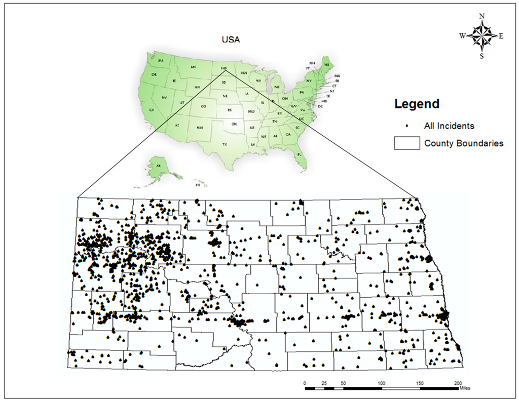
Figure 1.
Map of the study area with environmental incident locations, 2000–2014.
3. Methodology
This study used three different dimentions: temporal, spatial, and spatiotemporal analyses. The temporal analysis provides useful insight into hazardous material release management because this analysis can establish a baseline of activity and reveal new trends because data can be presented by the hour, day, month, and season, and year [18]. Temporal data could be shown using a simple line chart or spider plots because they can illustrate continuity and the chronological order of accidents [25]. Thus, of particular interest to this study is a spider graph, also known as a radar graph or star chart, because a spider graph has no specific beginning and ending time due to its circular nature. A spider graph is also easy to examine because it displays a high sequence of events and patterns by representing clockwise information [18,19]. In addition to this general temporal method, there are more sophisticated methods, including weighted time span analysis and percentage change [25]. Different types of hazardous material release accident statistics can be displayed using one of the above temporal methods.
In this study, the environmental incident data from across North Dakota has been mined to better understand the temporal nature of the accident. The study includes:
- Comparison of the temporal distribution of environmental incidents to all types of incidents and contaminants according to time of the day.
- Identification of the temporal distribution of environmental incident frequency according to the day of the week, month, season, and year.
Spatial statistical mapping is critical to understanding the relationship between spatial and temporal accidents [26,27] and spatial statistics are required for a set of techniques used to describe and model spatial data [28]. Spatial statistical analysis related to the oil spill can be carried out on a spatial database by integrating all the desired information and by generating data layers from the available sources which are updated by field verification [28]. Hot Spot analysis and Kernel density estimation (KDE) were carried out using Kernel density function. In addition to KDE, quadrant count method (QCM), and average nearest neighbor distance (ANND) are the most common methods for spatial pattern analysis [19]. These methods can be classified into two types: area-based technique (e.g., QCM) and distance-based technique (e.g., ANND and KDE) [29]. QCM relies on many characteristics of the distribution of the frequency of the observed numbers of points that are defined as sub-regions of the area of the study [30]. On the other hand, KDE and ANND methods use information of point spacing to characterize patterns [18]. The ANND method is based on the distance between each centroid and the centroid location of nearest neighbor and all nearest neighbor distances are a measure of average. In the ANND method, if the average value of the distance is less than the average of the hypothetical random distribution, the feature being analyzed is considered as clustered, whereas the feature is considered to be dispersed [31]. This study applied the KDE method to estimate the accident intensity (hot spot) of hazardous material releases at different counties in the state. The objective of KDE is to obtain a smooth and continuous estimation of the probability density for univariate or multivariate probability density using a weighted distance function. KDE visualizes the event clusters by representing the hot spots (presence of clusters) or cold spots (presence of fewer clusters) in the distribution of events [32,33].
The Hot Spot analysis assesses whether there are high or low values of environmental incidents clustered spatially within an identifiable boundary. The three major processes involved for analyzing desirable hot spot areas of environmental incidents include: 1) the collection of events, 2) clustered map using Getis-Ord Gi* function, and 3) the Kernel density estimation. Getis-Ord Gi* statistics work by looking at each different feature within the context of the neighboring feature. The feature has to have a high value and be surrounded by other high-value features in order to be a statistically significant Hot Spot. It compares the local sum of all features and its neighbor’s feature proportional to the sum of all features. A statistically significant Z-score results when the difference between a local sum and the expected local sum is too large to be the result of random chance. Z-score is the returned Getis-Ord Gi* statistic for each feature and a larger Z-score indicates a more intense clustering of high values (Hot Spot). The mathematical equation for calculating Gi* can be written as follows [34,35]:
where . is the attribute value x at events j over all n, is the spatial weight vector between feature i and j, and S is the sum of squared weight. The threshold distance (i.e., the proximity of the environmental incident to another) in this study was set to zero to indicate that all features were regarded as neighbors of all other features. We applied this threshold over the entire region of the study. Positive and negative Gi* statistics with high absolute values indicate the clusters of accident with high- and low-value events, respectively. If Gi* is close to zero, it implies a random distribution of events [32,33]. Finally, we performed KDE-based hot spot analysis in the populated field as GiZscore, which is available in the spatial analysis tool. This function calculates the magnitude per unit area using the hot spot feature from the GiZscore field. The output of this analysis is displayed as raster files by indicating the high and low cluster of accident occurrences [36].
Finally, spatiotemporal analysis is performed for a better interpretation of the environmental incidents in ND. There are various mapping and geospatial statistical analysis approaches for spatiotemporal analysis [37,38], which include animation, isosurface, and comap. Animation mapping is an old method that combines some snapshot into a continuous sequence and simulates the movement of the event [39]. The isosurface map analyzes and visualizes spatiotemporal data. This method creates a pattern from the events which occurred on an entire time unit such as day, week, or season so they can be seen at once. This map considers each incident occurrence as a point in space-time (x,y,t) that is used to estimate the probability density function (PDF) of f(x,y,t). Then, this function shows the likelihood of any incidents occurring at location (x,y) at a time (t). The advantage of this method is that it projects the density function in three-dimensional space [18]. On the other hand, comap is an extended version of Cleveland Coplot that visualizes changes in the value of variables over time by using small multiples of the diagram [40]. The method can investigate the relationship between the specific locations of environmental incidents and the variation exists between different time periods [18].
This study examines the effect of temporal change of oil spill accidents (e.g., hour, day, week, month, and season), and their effects on the spatial distribution of the selected environmental incidents. The comap can explore the spatial distribution of environmental incidents at an ordered time interval (e.g., Midnight to 4 a.m., 4 a.m. to 8 a.m.), during a day. Therefore, the hot spots of environmental incidents over space and time can be compared (univariate comap). Asgary et al. [18] suggested a step-by-step approach to create comap. Firstly, the range of each interval should be overlapped with each adjoin interval. Secondly, each interval needs to contain approximately the same number of incidents. The reason for these rules is to present output from the artifact of the classification process [18]. Finally, KDE analysis is performed for each interval for generating the Hot Spot maps. The advantage of this comap is that the changes over the entire time period are illustrated with a single visualization technique [38]. However, there can overlap class boundaries in comap in that a similar distribution of data can be located in several classes. This is a limitation of the application of comap technique [20]. The classification method such as Jenks Natural Breaks can improve this limitation by reducing the variance within each class [41].
4. Results
4.1. Environmental Incident Analysis
General environmental incident data set used for the present study includes over 3000 incidents occurred between 2000 and 2014. Since the data includes many types of incidents and contaminants, dominant incident types and contaminants are illustrated using bar graphs to visualize and compare the frequency of occurrence of the top 10 environmental incidents in the ND. Figure 2 and Figure 3 show the top 10 environmental incidents by type of incident and contaminant. First, in terms of type of incident, the State is found to have a high number of tank related accidents accounting for about 25% of total incidents followed by vehicle accidents with 18.64% share, pipeline 10.47% share, whereas, valve, hose, fire, transformer are found to have relatively lower percent shares, which account for 1.18%, 1.59%, 1.72%, and 1.72%, respectively. In addition, as shown in Figure 3, it can be inferred that diesel accounts for 21.27% of the total type of contaminant share, followed by crude oil for 21.13%, while unknown contaminants account for 1.11% of the total contaminant impact. Similarly, mineral oil accounted for 1.22%, petroleum accounted for 1.38%, ammonia accounted for 1.62%, gasoline accounted for 2.26%, produced water/saltwater accounted for 3.95%, hydraulic fluid/oil accounted for 5.40% of the total release.
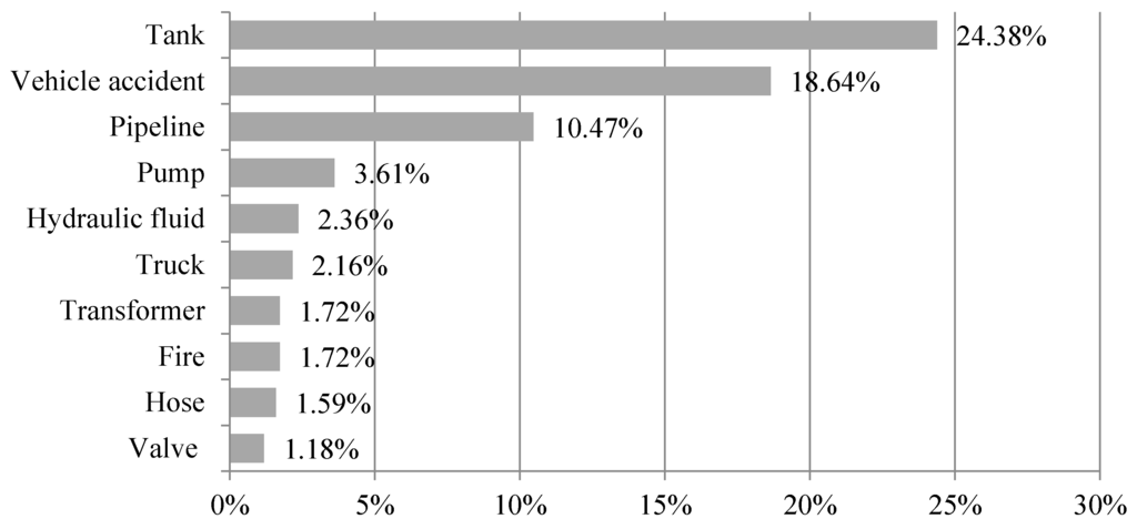
Figure 2.
The percentage share of top 10 incident types.
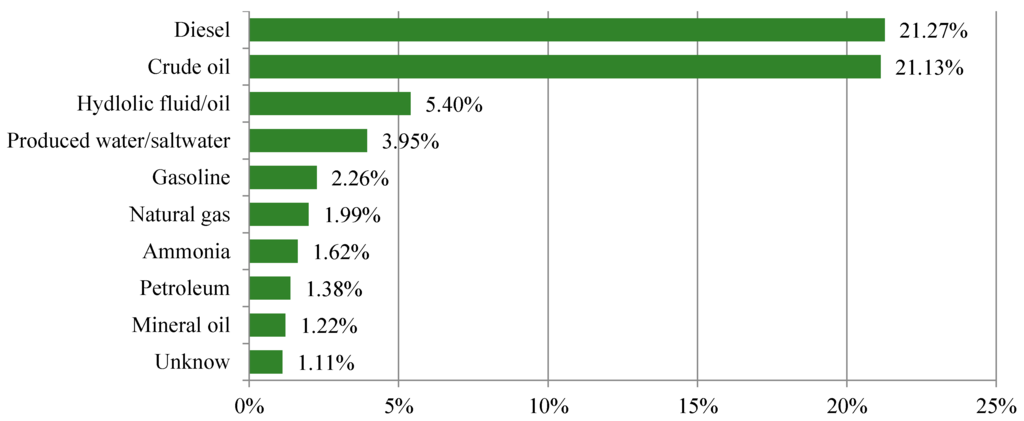
Figure 3.
The percentage share of top 10 contaminant types.
4.2. Temporal Analysis
This section shows the annual pattern of the accidents involving hazardous material releases. According to the line graph (see Figure 4), the level of number of oil spills were steady and below 200 per year until 2010. However, substantial increases observed in after 2010 with an exponentially increasing rate. There were 290 incidents in 2011 and the total number of oil spills jumped to 300 incidents in 2012. The increases continued, with the number of accidents jumping to 590 incidents per year in 2013 reaching almost 800 incidents per year in 2014. These devastating numbers unfortunately indicate that the environmental and emergency management had already lost the control of the problems. The rate of accident level shows the same trend as the rate of oil production [42].
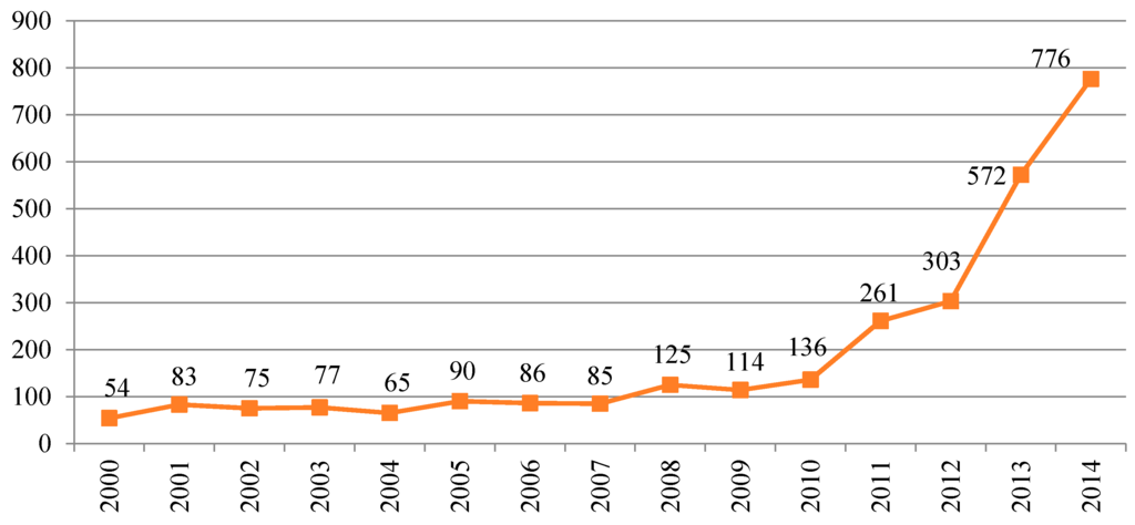
Figure 4.
Annual pattern of environmental incidents in ND, 2000–2014.
Spider graphs are presented in Figure 5a–d to illustrate the temporal pattern of oil spills, including hourly, daily, monthly, and seasonally in North Dakota (to determine the four seasons, meteorological seasons in the Northern Hemisphere are used). First, in terms of the hourly pattern (Figure 5a), most hazardous material releases occurred between 7 a.m. and 5 p.m. with the peak occurring between 2 p.m. and 3 p.m. Figure 5b also shows that environmental incidents are more frequent during weekdays, from Mondays to Fridays, with peaks on Tuesdays, Wednesdays, and Thursdays. Saturdays and Sundays have the least number of environmental incidents. Interestingly, our incident database mirrors what was observed in a 12-year study of hazardous materials incidents in Chester County in Pennsylvania [3] and six-month pilot study conducted in Australia [6]. The highest number of environmental incidents occur in the July, September, and October. The fewest oil spill accidents occur from December to May (Figure 5c). Lastly, Figure 5d also shows the seasonal pattern of oil spill incidents. There is an excessively high number of accidents occur in the summer and the lowest number of the accidents occur in the winter and spring.
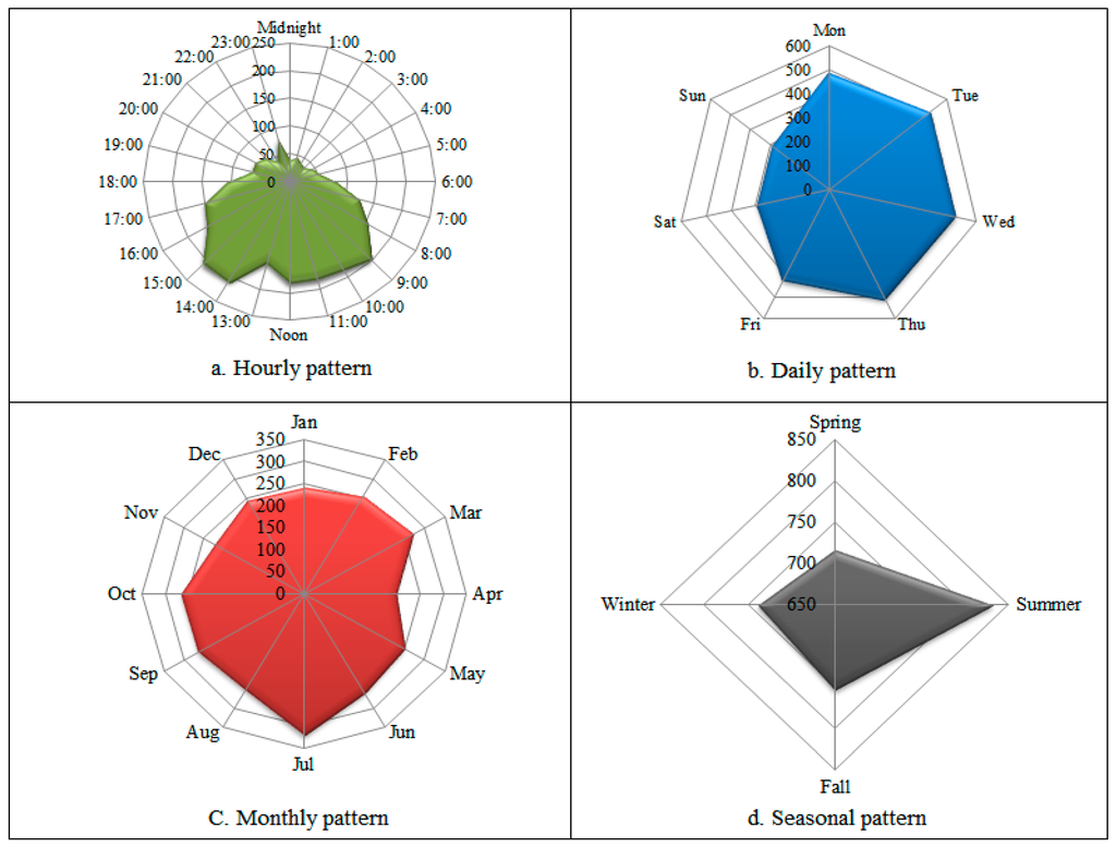
Figure 5.
Temporal pattern of environmental incidents in ND, 2000–2014.
4.3. Spatial Analysis
The Hot Spot and Kernel density surfaces were obtained for total general environmental incidents as a whole during the period between 2000 and 2014. The Hot Spots were estimated using the Getis–Ord Gi* function followed by the event calculation. This function identifies spatial clusters of high intensity (Hot Spots) and of low intensity (cold spots) regions. Dark blue color code indicates the most affected areas, whereas light yellow color code indicates the least affected regions in Figure 6. The following figure shows the results of the Kernel density analysis for all environmental incidents in the ND during the period between 2000 and 2014.
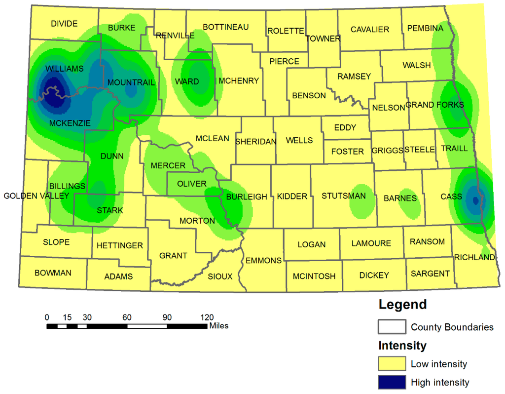
Figure 6.
Spatial analysis (Kernel density estimation), 2000–2014.
KDE is performed at different spatial scales for oil spill accidents. Executing KDE on the whole of North Dakota is useful for identifying primary Hot Spot regions where environmental incidents are not frequent. Findings indicate that unclassified total environmental incidents are particularly clustered around two areas. One of the Hot Spot areas is located either on oil production sites or undeveloped areas (e.g., road, land), which include William, McKenzie and Mountrail counties. One possible reason may stem from the fact that major roads in these counties are in poor condition or outdated, thus, vehicle accidents tend to happen more. This issue is also addressed in the report of Upper Great Plains Transportation Institute [43]. The other Hot Spot is located around the City of Fargo (Cass County), where the population density is significantly high and urban activities are taking place more. The spatial patterns of environmental incidents analyzed in this study enable policy makers to quickly and aesthetically determine the locations, where statistically significant number of accidents occurs.
4.4. Spatiotemporal Analysis
The results presented so far have highlighted that environmental incidents are spread unevenly in either space or time, where this unevenness varied by the pattern of environmental incidents. Although the previous spatial analysis map provides insight into the temporal and spatial patterns of environmental incidents separately, it cannot provide information about the interaction between space and time [18]. In this section, we create and use the comap to determine if the same level of environmental incident risk area is subject to temporal fluctuations of environmental incidents. In the comap (Figure 7), univariate spatiotemporal plots are created for each incident during each time interval with two hours overlapping (such as midnight to 5 a.m., 3 a.m. to 8 a.m.) due to avoiding temporal boundary problem. These plots are numbered from 1 to 6 so that we can identify and interpret the spatial and temporal pattern of the environmental incidents. Figure 7 shows the spatial density of all environmental incidents in North Dakota counties by the hour. As depicted in Figure 7, the density of environmental incidents in North Dakota changes by time (hours) in that there are variations in incident distribution throughout the day. The environmental incident intensity is lower in the early hours of the evening and late hours of the day. Early and late hours of the mornings seem to have a denser pattern of environmental incidents. After peaking in the morning, environmental incidents decrease in terms of the density over time. On the other hand, in terms of spatial pattern, the Hot Spots indicate a dynamic pattern of behavior, particularly around those areas where a massive amount of oil is produced periodically (e.g., Williams, Mckenzie, and Mountrail), as well as in the City of Bismarck (in Burleigh County), the City of Fargo (in Cass County), and the City of Grand Forks (in Grand Forks County). Williams, Mckenzie, and Mountrail are found to have a greater incident density in the morning and have reduced density from midnight to the early hours of the morning. Fargo has a more dynamic density pattern across time. The environmental incident pattern in Fargo gradually increases, peaking during the early morning hours and early in the afternoon, then decreasing as the day continues.
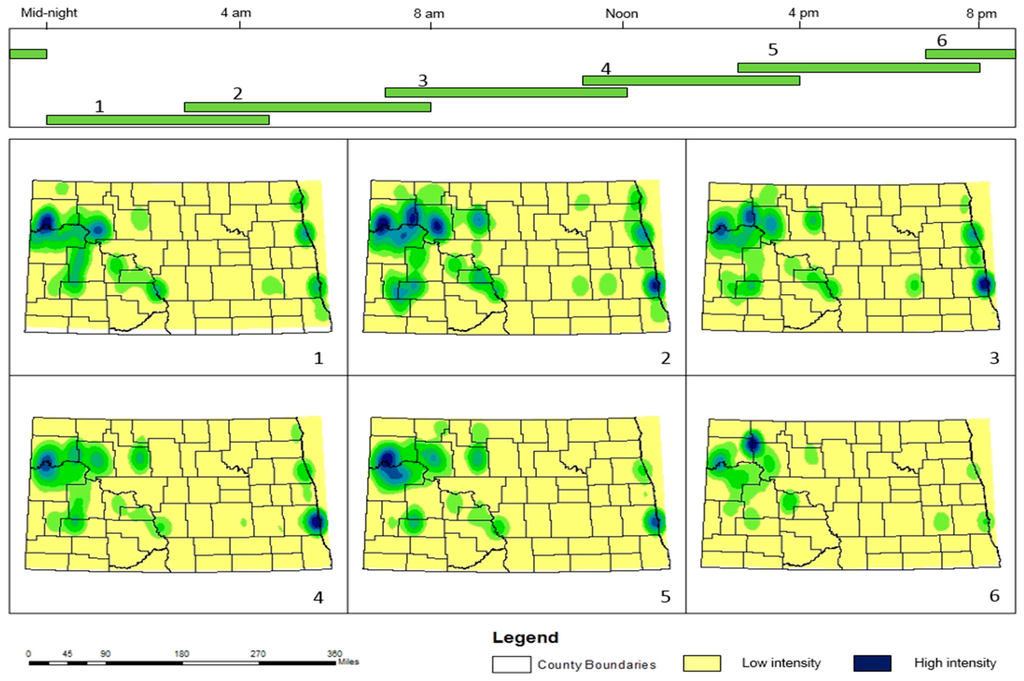
Figure 7.
Univariate comap for environmental incidents (by hour); Interval 1 is from midnight to 5 a.m., Interval 2 is from 3 a.m. to 8 a.m., Interval 3 is from 7 a.m. to noon, Interval 4 is from 11 a.m. to 4 p.m., Interval 5 is from 3 p.m. to 8 p.m., and Interval 6 is from 7 p.m. to midnight, respectively.
To explain the more spatiotemporal relationship between county and incident, we also performed a regression analysis of oil production level and the number of incidents for each county. The result shows that the number of all environmental incidents in North Dakota appears to be closely correlated with the rate of oil production. To assess this, the total amount of oil production from 2000 to 2014 was calculated for the counties, where incidents were reported. The linear rate of oil production for each county is plotted against the number of total environmental incidents in that county. As shown in Figure 8, the least-square linear relationship was significant by R2 = 0.6621 and p-value = 0.000229. This pattern indicates that there is a high risk of environmental incidents in the counties that produce the most oil.
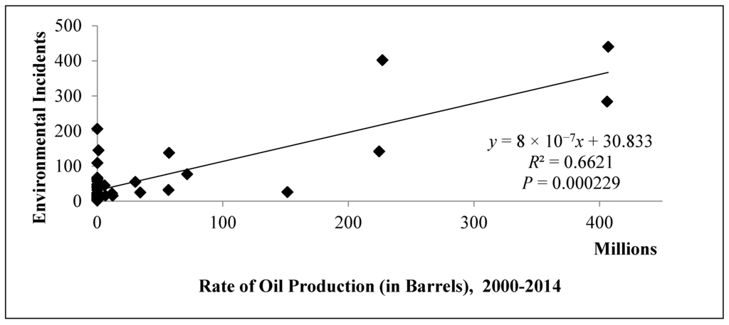
Figure 8.
Regression analysis of oil production vs. environmental incidents in North Dakota.
5. Conclusions
Spatiotemporal analysis adds value to the existing method of identifying the hazardous material release patterns in time. When coupled with spatially related data, spatiotemporal visualization using GIS, dynamic mapping and the simulation of past environmental incidents can provide valuable insights into understanding the possible root causes or locations of environmental incidents [18]. Moreover, GIS can also be used to analyze and visualize spatial data to find out potential patterns in the incident data, which can be effectively used emergency management planning. In this study, all available information about environmental incidents was used to identify the spatiotemporal pattern of hazardous material releases from 2000 to 2014. Our analysis clearly shows that hazardouse waste- related environmental incidents follow spatial and temporal patterns. This study also emphasizes multi-dimensional data collection and significies the effective use of data-driven public decision making proceses for mitigating the oil spills and better environmental and emergence management.
Based on the results, we can conclude: (a) tank, vehicle accident and pipeline were the dominant types of incidents and the most-frequently released contaminants were diesel and crude oil; (b) environmental incidents occurred most often in the morning and afternoon, during the work week, and during warm weather; (c) Kernel density estimation shows that hot spot density tends to be distributed around oil production sites in undeveloped areas as well as in areas of high population density where more urban activities are taking place; (d) a comap (univariate spatiotemporal plot) showed that there were variations in incident distribution throughout the day; and (e) there was a spatial relationship between the number of environmental incidents and the amount of oil production associated with each county.
The analytical and conceptual findings of this study will be instrumental in mitigating the risks associated with environmental incidents. To improve the environmental safety and emergency management performance across the state, planners and decision makers must identify and consider these spatiotemporal patterns and use them in formulating policies regarding the handling, transport and storage of hazardous materials. In fact, current results indicate that the awareness and effectiveness of emergency management and environmental policy making in the state is very outdated, lousy, and, questionable. A thorough professional understanding and impartial but society and environmentally friendly regulations, and actions are immediately required to deal with hazardous material incidents. The policy focus should directly address prevention efforts on specific times of day, days of the week, and seasons when accidents happen more frequently. From the analysis results, one can easily find the problematic area of oil spill accident. For example, tank, pump, hose, and valve related accidents are majorly attributed to construction or oil well sites that have high impact on release of crude oil, saltwater, and hydraulic fluid/oil. Oil spills that were based on diesel and gasoline (final products) are usually attributed to the transportation related root causes. Therefore, adequate staffing and resources should be allocated for the time and locations where more accidents happens so that the probability of accidents can be reduced. Allocating resources to the right place and at the right time is critical to enhance the incident response time [3], as well as ensuring safety during the operation of facilities and transporters. As the well-known mantra indicates, what gets measures gets managed, the emergency and contingency plans should be organized around the findings of analytical (data science) efforts such as i.e., collecting, storing, and sharing datasets) through analytics as well as visualization.
While this study demonstrated spatiotemporal variations of the oil spills in the state of North Dakota, the current focuses lacked the analytical understanding about the specific types of incidents and contaminants, because the primary focus was to provide an overview of spatiotemporal pattern of unclassified environmental incidents. Therefore, the specific types of the incidents will be further analyzed by classifying the most frequent type of incidents and contaminants such as storage or transportation. Future work should also corroborate the existing results and extend our understanding of the current problem. We can examine the relationship between environmental incidents, socioeconomic characteristics of different areas and the environmental incidents that occur there. Another possible future extension would be focusing on the volume of environmental incidents to clarify the impact of a hazardous material release to the environment and land use.
Acknowledgments
The research was partially funded by the Mountain-Plains Consortium (MPC), one of the University Transportation Centers of U.S. Department of Transportation.
Author Contributions
Y.S. Park and H. Al-Qublan conceived and designed the research plan; Y.S. Park performed the experiments; Y.S. Park and G. Egilmez analyzed the data; Y.S. Park and E.S. Lee contributed reagents/materials/analysis tools; Y.S. Park and E.S. Lee wrote the paper.
Conflicts of Interest
The authors declare no conflict of interest. The founding sponsors had no role in the design of the study; in the collection, analyses, or interpretation of data; in the writing of the manuscript, and in the decision to publish the results.
Abbreviations
The following abbreviations are used in this manuscript:
| KDE: | Kernel density estimation |
| GIS: | geographic information systems |
References
- Duan, W.; Chen, G.; Ye, Q. The situation of hazardous chemical accidents in China between 2000 and 2006. J. Hazard. Mater. 2011, 186, 1489–1494. [Google Scholar] [CrossRef] [PubMed]
- Li, Y.; Brimicombe, A.; Ralphs, M.P. Spatial data quality and sensitivity analysis in GIS and environmental modelling: the case of coastal oil spills, Computer. Environ. Urban Syst. 2000, 24, 95–108. [Google Scholar] [CrossRef]
- Shorten, C.; Galloway, J.; Krebs, J.; Fleming, R. A 12-year history of hazardous materials incidents in Chester County, Pennsylvania. J. Hazard. Mater. 2002, 89, 29–40. [Google Scholar] [CrossRef]
- United States Coast Guard, National Response Center. 2014. Available online: http://www.nrc.uscg.mil/ (accessed on 5 May 2015).
- Gunster, D.; Gillis, C.; Bonnevie, N.; Abel, T. Petroleum and hazardous chemical spills in Newark Bay, New Jersey, USA from 1982 to 1991. Environ. Pollut. 1993, 82, 245–253. [Google Scholar] [CrossRef]
- Winder, C.; Tottszer, A.; Navratil, J.; Tondon, R. Hazardous materials incidents reporting: Results of nationwide trial. J. Hazard. Mater. 1992, 31, 119–134. [Google Scholar]
- Burgess, J.; Pappas, G.; Robertson, W. Hazardous materials incidents: The Washington Poison Center experience and approach to exposure assessment. J. Occup. Environ. Med. 1997, 39, 760–766. [Google Scholar] [CrossRef] [PubMed]
- Ianc, C. Factors affecting the cost of oil spills. In Proceedings of the GAOCMAO Conference, Muscat, Oman, 12–14 May 2002.
- Giesppe, S.; Helfried, O.; Pietro, P.; Kalliopi, R. Forests of the Mediterranean region: Gaps in knowledge and research needs. For. Ecol. Manag. 2000, 132, 97–109. [Google Scholar]
- Asgary, A.; Ghaffari, J.; Levy, J. Spatial and temporal analyses of structural fire incidents and their causes: A case of Toronto, Canada. Fire Saf. J. 2010, 45, 44–57. [Google Scholar] [CrossRef]
- Plug, C.; Xia, J.; Caulfield, C. Spatial and temporal visualisation techniques for crash analysis. Accid. Anal. Prev. 2011, 43, 1937–1946. [Google Scholar] [CrossRef] [PubMed]
- Pew, K.; Larsen, C. GIS analysis of spatial and temporal patterns of human-caused wildfires in the temperate rainforest of Vancouver Island, Canada. For. Ecol. Manag. 2001, 140, 1–18. [Google Scholar] [CrossRef]
- Jaiswal, R.; Mukherjee, S.; Raju, K.; Saxena, R. Forest fire risk zone mapping from satellite imagery and GIS. Int. J. Appl. Earth Obs. Geoinf. 2002, 4, 1–10. [Google Scholar] [CrossRef]
- Chainey, S.; Tompson, L.; Uhlig, S. The utility of hotspotmapping for predicting spatial patterns of crime. Secur. J. 2008, 21, 4–28. [Google Scholar] [CrossRef]
- Laurian, L.; Funderburg, R. Environmental justice in France? A spaio-temporal analysis of incinerator location. J. Envrion. Plan. Manag. 2014, 53, 424–446. [Google Scholar] [CrossRef]
- Wang, D.; Ding, W.; Lo, H.; Stepinski, T.; Salazar, J.; Morabito, M. Crime hotspot mapping using the crime related factors—A spatial data mining approach. Appl. Intell. 2013, 39, 772–782. [Google Scholar] [CrossRef]
- Bowers, K. Book Review. In Mapping and Analysing Crime Data: Lessons from Research and Practice; CRC Press: Boca Raton, FL, USA, 2004; p. 47. [Google Scholar]
- Gerber, M. Predicting crime using Twitter and Kernel density estimation. Decis. Support Syst. 2014, 61, 115–125. [Google Scholar] [CrossRef]
- Cao, G.; Wang, S.; Hwang, M.; Padmanabhan, A.; Zhang, Z.; Soltani, K. A scalable framework for spatiotemporal analysis of location-based social media data. Environ. Urban Syst. 2015, 51, 70–82. [Google Scholar] [CrossRef]
- Corcoran, J.; Higgs, G.; Brunsdon, C. The use of spatial analytical techniques to explore patterns of fire incidence: A South Wales case study. Comput. Environ. Urban Syst. 2007, 31, 623–647. [Google Scholar] [CrossRef]
- Maher, M.; Mountain, L. The identification of accident blackspots: A comparison of current methods. Accid. Anal. Prev. 1988, 20, 143–151. [Google Scholar] [CrossRef]
- Liang, L.; Hua, L.; Ma’som, D. Traffic accident application using geographic information system. J. East. Asia Soc. Transp. Stud. 2005, 6, 3474–3589. [Google Scholar]
- Oliveira, E.; Silveira, B.; Alves, F. Support mechanisms for oil spill accident response in costal lagoon areas (Ria de Aveiro, Portugal). J. Sea Res. 2014, 93, 112–117. [Google Scholar] [CrossRef]
- North Dakota Department of Health. North Dakota Hazardous Waste Compliance Guide; Division of Waste Management: Bismarck, ND, USA, 2012.
- Boba, R. Crime Analysis and Crime Mapping; Sage: Beverly Hills, CA, USA, 2005. [Google Scholar]
- Haining, R. Spatial Data Analysis: Theory and Practice; University of Cambridge Press: Cambridge, UK, 2003. [Google Scholar]
- Levin, N.; Kim, K.; Nitz, L. Spatial analysis of Honolulu motor vehicle crashes: I. spatial patterns. Accid. Anal. Prev. 1995, 27, 663–674. [Google Scholar] [CrossRef]
- Prasannakumar, V.; Vijith, H.; Charutha, R.; Geetha, N. Spatio-temporal clustering of road accidents: GIS based analysis and assessment. Procedia Soc. Behav. Sci. 2011, 21, 317–325. [Google Scholar] [CrossRef]
- Haggett, P.; Cliff, A.; Frey, A. Locational Analysis in Human Geography; Edward Arnold: London, UK, 1997. [Google Scholar]
- Gatrell, A.; Bailey, T.; Diggle, P. Spatial point pattern analysis and its application in geographical epidemiology. Trans. Inst. Br. Geogr. 1996, 21, 256–274. [Google Scholar] [CrossRef]
- Mitchell, A. Guide to GIS Analysis; ESRI Press: Redlands, CA, USA, 2005; Volume 2. [Google Scholar]
- Silverman, B.W. Density Estimation for Statistics and Data Analysis. Number 26 in Monographs on Statistics and Applied Probability; Chapman & Hall: London, UK, 1986. [Google Scholar]
- Bailey, T.C.; Gatrell, A.C. Interactive Spatial Data Analysis; Routledge: Abingdon-on-Thames, UK, 1995. [Google Scholar]
- Ord, J.; Getis, A. Local Spatial Autocorrelation Statistics: Distribution Issues and an Application. Geogr. Anal. 1995, 27, 286–306. [Google Scholar] [CrossRef]
- Getis, O.J. Testing for local spatial autocorrelation in the presence of global autocorrelation. J. Reg. Sci. 2001, 41, 411–432. [Google Scholar]
- DeGroote, J.; Sugumaran, R.; Brend, S.; Tucker, B.; Bartholomay, L. Landscape, demographic, entomological, and climatic associations with human disease incidence of West Nile virus in the state of Iowa. Int. J. Health Geogr. 2008, 7, 1. [Google Scholar] [CrossRef] [PubMed]
- Finkenstadt, B.; Held, L.; Ishan, V. Statistical Methods for Spatiotemporal Systems; Chapman and Hall/CRC: Boca Raton, FL, USA, 2007. [Google Scholar]
- Ugarte, M. Statistical methods for Spatio-temporal systems. J. R. Stat. Soc. Ser. A 2007, 170, 1182. [Google Scholar] [CrossRef]
- Curtis, A.; Leiner, M.; Hanlon, C. Using hierarchical nearest neighbor analysis and animation to investigate the spatial and temporal patterns of raccoon rabies in West Virgina, PA, USA. In Geographic Information Systems and Health Applications; Idea Group Publishing: Hershey, PA, USA, 2002; pp. 155–171. [Google Scholar]
- Brunsdon, C. The comap: Exploring spatial pattern via conditional distributions. Comput. Environ. Urban Syst. 2001, 25, 53–68. [Google Scholar] [CrossRef]
- Jenks, G.F. The data model concept in statistical mapping. Int. Yearbook Cartogr. 1967, 7, 186–190. [Google Scholar]
- U.S. Department of Energy. North Dakota Field Production of Crude Oil (Thousdands Barrels Per Day); Energy Information Administration: Washington, DC, USA, 2014.
- UGPTI. Infrastructure Needs: North Dakota’s County, Township and Tribal Roads and Bridges: 2015–2034; Upper Great Plains Transportation Institute: Fargo, ND, USA, 2014. [Google Scholar]
© 2016 by the authors; licensee MDPI, Basel, Switzerland. This article is an open access article distributed under the terms and conditions of the Creative Commons Attribution license ( http://creativecommons.org/licenses/by/4.0/).