Article

Enhancing 3D MRI-Based Necrotic Core Segmentation in Glioblastoma Using Activation Functions in Deep Learning


by
Mushtaq Mahyoob Saleh
1,*,
Eltahir Mohamed Hussein
1,
Musab Elkheir Salih
1 and
Mohamed A. A. Ahmed
1,2
1
Biomedical Engineering Department, College of Engineering, Sudan University of Science and Technology, P.O. Box 407, Khartoum 11111, Sudan
2
Electrical & Electronic Engineering, Professional Construction & HE Engineering, University Centre Colchester, Colchester Institute, Colchester CO3 3LL, UK
*
Author to whom correspondence should be addressed.
Informatics 2026, 13(7), 118; https://doi.org/10.3390/informatics13070118
Submission received: 25 May 2026 / Revised: 1 July 2026 / Accepted: 9 July 2026 / Published: 20 July 2026
(This article belongs to the Section Medical and Clinical Informatics)

Abstract

Precise brain tumour delineation is vital for therapy protocols and tracking. However, standard Rectified Linear Units (ReLU) struggle to capture subtle necrotic-core variations due to zero-gradient behaviour in the negative domain. To address this, we present a controlled benchmark of 12 activation functions within a fixed Residual 3D U-Net using the Brain Tumour Segmentation (BraTS) 2020 dataset. In the single-run benchmark, Swish achieved the best necrotic-core (NCR) Dice (0.676; +2.0% over ReLU, p < 0.01), while TanhExp attained the highest whole-tumour accuracy (0.879). To test the reliability of these single-run results, the four functions central to our claims were retrained across three random seeds. This analysis confirmed a small but consistent NCR advantage for the smooth and adaptive functions—Swish (0.677 ± 0.003) and PReLU (0.678 ± 0.004) over ReLU (0.661 ± 0.012; pooled p < 0.001)—with Swish among the most stable functions in this region. By contrast, the apparent single-run differences in the enhancing tumour, and the underperformance of PReLU, did not generalise across seeds, indicating that activation-function effects in this task are concentrated in the necrotic core and that single-seed comparisons can be misleading. Crucially, Swish achieved these gains with zero additional trainable parameters and only a ~1% training latency penalty on common hardware. Replacing ReLU with Swish offers a cost-effective, architecture-preserving strategy to improve segmentation reliability and boundary delineation. Ultimately, this zero-cost architectural modification is a promising, preliminary step towards more reliable automated tumour delineation, pending prospective validation on multi-institutional data and expert radiological assessment.

1. Introduction

Brain tumours are complex diseases which, if not treated, can severely affect a patient by causing malfunctioning in several organs and systems of the body. The brain is the main organ that controls each operation of the body. Therefore, the unusual growth of brain tissue, whether benign or malignant in nature can exert pressure on parts that control vital activities. This pressure can cause prolonged pain and several neurological disorders that may occur in any part of the body and, in severe conditions, may also lead to death.
There exist two major classes of brain tumours: primary and secondary tumours. Primary tumours originate from glial cells and may occur anywhere in the brain. These tumours seldom metastasise to other parts of the body, even though they may be benign or malignant. The most common primary tumour types include pituitary tumours, meningiomas, and gliomas. On the other hand, secondary tumours, also referred to as metastatic tumours, arise due to cancers that have spread from other parts of the body into the brain or spinal cord [1].
According to the World Health Organisation (WHO), brain tumours are categorised into four grades, ranging from Grade I to Grade IV. Grade IV represents the most aggressive and malignant form, which has a high growth rate and malignancy level, while Grade I is the initial stage, with moderate growth [2,3]. Various types of brain tumours, commonly referred to as gliomas, have been noted. Among these, low-grade and high-grade gliomas are the most common and aggressive types, characterised by rapid growth and serious effects on the patient. Glioblastoma is considered a Grade IV tumour by the WHO. In addition, there is a very high possibility of recurrence after treatment [4].
Accurately identifying and localising brain tumours remains difficult due to their heterogeneous morphology, variable sizes, and diverse anatomical locations. Therefore, Magnetic Resonance Imaging (MRI) has been widely utilised to overcome such challenges, as it provides rich structural information and excellent soft-tissue contrast. A typical MRI examination includes four main imaging modalities: T1-weighted scans, T1ce-weighted scans following contrast administration, T2-weighted scans, and Fluid-Attenuated Inversion Recovery (FLAIR) scans. Each modality provides complementary information, allowing for a comprehensive investigation of tumour characteristics [5,6,7].
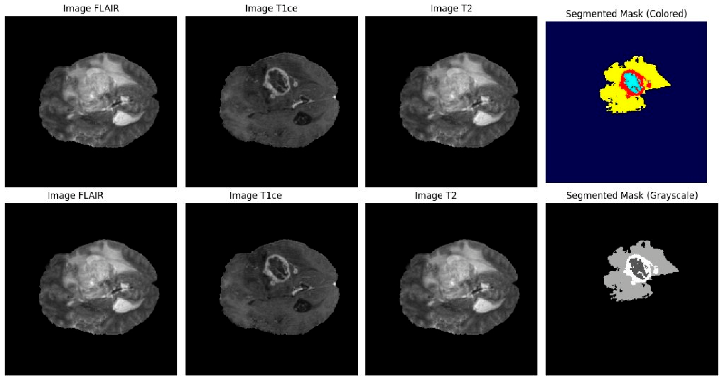
Figure 1 shows all four MRI modalities with grey-scale and colour-coded segmentation maps of tumour regions. In these visualisations, oedema, indicating fluid accumulation in brain tissue, with no active tumour cells, is shown in yellow. The enhancing-tumour region, typically containing a high-grade malignancy, is coloured in red. The colour blue indicates the non-enhancing-tumour region, which does not take up the contrast material and may contain necrotic tissue; however, viable tumour cells remain and can proliferate, leading to continued tumour growth.
FLAIR imaging, which is derived from T2-weighted sequences, increases the contrast of oedema by suppressing the Cerebrospinal Fluid (CSF) signal, making it dark. This is quite sensitive in detecting oedema and non-enhancing areas of the tumour. In routine T2-weighted images, both CSF and fluid-containing tissues appear bright; therefore, oedema can be well delineated. T1-weighted images, in which CSF is dark and tumour contrast is low, are mainly useful for detailed anatomical information. Following contrast administration, usually with gadolinium-based compounds, T1ce images highlight regions with blood–brain barrier disruption, whereas areas of oedema and non-enhancing tumour are relatively unenhanced.
Brain tumour segmentation can be achieved using various conventional methods [7], such as thresholding [8], watershed [9], region growing [10], edge detection [11], and clustering [8,12]. These methods are time-consuming and labour-intensive. Moreover, they struggle to cope with the complexities of brain tumours, given the challenges posed by volumetric data, tumour position and volume, low contrast ratios, and intensity variations. Because traditional algorithms rely on manually crafted rules, they inherently lack the flexibility to adapt to the immense morphological diversity of gliomas. Currently, image processing in the medical field has undergone a revolution driven by Artificial Intelligence (AI), Machine Learning (ML), and Deep Learning (DL), which have resolved issues encountered with other methods. By automatically learning hierarchical spatial features directly from the volumetric data, DL models can successfully navigate the highly variable contexts that confound classical methods. Several deep learning architectures, such as AlexNet [13], VGGNet [14], InceptionNet [15], XceptionNet [16], U-Net [17], ResNet [18], and DenseNet [19], have been applied to medical imaging tasks. Among these models, the U-Net [17] has gained widespread recognition for its robust feature extraction from images, along with its U-shaped structure, which effectively encodes both global and local information through an encoder–decoder architecture with skip connections.
Convolutional neural networks (CNNs) form the building blocks of the U-Net. The U-Net is a deep learning technique that employs volumetric data, such as 3D MRI images in the BraTS challenge, to learn the spatial hierarchy of features. The brain tumour segmentation (BraTS) challenge [20] is an annual initiative conducted under the Medical Image Computing and Computer Assisted Intervention (MICCAI) society, with the aim of advancing research related to brain tumour segmentation. This society was created in 2012.
U-Net employs CNNs that learn features step by step, progressing from low-level features such as textures to high-level features representing complex patterns [21]. Activation functions, an important component of deep learning models, provide an effective means of replicating such complex patterns. Choosing the appropriate activation function is critical to enhancing the accuracy of segmentation, improving training speed, and minimising the vanishing gradient problem. Swish [22], ReLU [23], Leaky ReLU [24], PReLU [25], ELiSH [26], HardELiSH [26], ELU [27], GELU [28], Mish [29], TanhExp [30], Logish [31], and Smish [32] are some commonly used activation functions in deep learning methods for tumour segmentation tasks [33]. While dealing with high-dimensional MRI data, any advancement in computational time, gradient backpropagation, characteristic extraction, or rectifying the vanishing gradient issue can prove beneficial in improving the performance of the proposed methodology. This eventually leads to accurate, effective, and more reliable brain tumour segmentation. Therefore, selecting the proper activation function is critical for achieving maximum performance.
Although many improvements have been achieved through residual connections, cascaded connections, and ensemble learning architectures, the standard activation function used in most existing models for 3D image segmentation is the ReLU (Rectified Linear Unit). Although the ReLU activation function is efficient during computation, it is affected by drawbacks such as the zero gradient problem when inputs are negative, and another issue referred to as the “dying ReLU” problem. When processing negative inputs—which frequently occur in normalised, hypointense regions like the necrotic core—ReLU neurons stop updating, leading to a loss of subtle boundary information. To fill this research gap, this study aims to assess twelve different activation functions within a fixed and standard 3D U-Net architecture (ImprovedUNetED) using the BraTS2020 dataset for brain tumour segmentation.
To our knowledge, this is the first study to isolate the activation function as a single controlled variable across a panel of twelve functions within a fixed volumetric residual U-Net, and to evaluate its effect at the level of individual glioma sub-regions—in particular the necrotic core, whose hypointense, irregular boundaries are the most sensitive to how negative pre-activations are treated. Prior work typically varies the activation alongside architectural or training changes, confounding its individual contribution; by freezing all other factors, we attribute the measured differences solely to non-linearity.
A key strength of this study is the controlled experimental design, where all architectural and training hyperparameters remain constant. Consequently, this research evaluates how different activation functions affect convergence, generalisation, overlap, and boundary detection during tumour segmentation.
The contributions of this study are threefold:
  • A controlled and reproducible evaluation of twelve different activation functions in a residual 3D U-Net architecture.
  • A thorough evaluation using overlap and boundary measures, including the Dice Score, IoU, sensitivity, Specificity, and Hausdorff Distance (HD95).
  • Quantitative evidence, validated across three random seeds, that the effect of the activation function is region-specific and concentrated in the necrotic core, where smooth or adaptive functions (Swish and PReLU) yield a small but consistent and more stable improvement over ReLU; differences in the enhancing tumour, tumour core and whole tumour—and the apparent single-run underperformance of PReLU—did not generalise across seeds, underscoring the importance of multi-seed evaluation for activation-function comparisons.
  • Unlike processing slices individually, the 3D U-Net architecture uses three-dimensional convolution to extract features from the entire volume, leveraging the full spatial context of the input data. Because the 3D U-Net directly extracts hierarchical features from volumetric data, it is found to be more robust and efficient than the 2D U-Net architecture. This approach improves the model’s overall performance significantly [34,35,36].

2. Literature Review

Recently, deep learning has become the basis for automatic brain tumour segmentation. The driving force behind this progress is the availability of standardised benchmark datasets, such as the BraTS Challenge. The initial results published in BraTS showed the efficacy of multimodal MRI and algorithmic fusion techniques for image segmentation when compared to conventional image processing methods.
Some research works have utilised the 3D U-Net for segmenting brain tumours. While the 3D U-Net has become the de facto standard for this task, researchers continually grapple with optimising its architecture to balance computational cost and segmentation accuracy. For example, Fernando and Tsokos [37] (2023) combined statistical techniques with deep learning to segment brain tumours from 3D MRI images, achieving higher accuracy than previous methods. However, their approach was hindered by slow convergence rates and a susceptibility to local optima. Ullah et al. [38] (2021) developed a technique to enhance brain MRI images as a preprocessing step for brain tumour segmentation using the 3D U-Net, achieving high Dice coefficients. Nevertheless, their results did not surpass existing state-of-the-art techniques.
Feng et al. [39] (2020) proposed an ensemble of 3D U-Net models combined with a multivariate linear regression approach to enhance segmentation performance; however, their methodology could lead to overfitting given the small sizes of the datasets used. Ballestar and Vilaplana [40] (2020) explored the architectures of 3D U-Net models using patch-based methods along with model ensembles for improvement, but they noted that their methodology could potentially produce more false positives, especially in the enhancing-tumour area.
A 3D U-Net-based approach for both segmentation tasks and survival analysis was proposed by Wang et al. [41] (2020), improving the segmentation result, but with limited results for survival analysis. Lastly, in one of the highest impacts in this area, Kamnitsas et al. [42] proposed DeepMedic, which is a 3D CNN for brain tumour segmentation, comparing the power of volumetric information over the 2D slice-based approaches. Their updated version using residual learning played an important role in advancing this area, but with the drawback that their approach depends on high-quality training data with limited results in cases with differences between training and testing distributions.
To lay a foundation for research in the area, challenges such as Multimodal brain tumour segmentation (BraTS) are crucial, as they define a common benchmark for segmentation approaches through standardised datasets.
The BraTS annual competitive setting has played a vital role in promoting innovation, which directly resulted in the creation of increasingly more accurate and innovative deep learning methods, thus reflecting the chronological development of the field. A chronological summary of these key BraTS challenge studies, including their specific contributions and limitations, is outlined in Table 1.
Nevertheless, the above advances, despite being effective for the model’s overall performance, are not satisfactory for the segmentation accuracy on the sub-regions of the tumour and the enhancement and necrotic regions that have more severe issues with imbalance and boundaries. This is because most current solutions focus on the architectural complexity, the loss function design, and the data augmentation techniques, while predominantly using the conventional activation function such as ReLU or Leaky ReLU.
Despite good optimisation properties of some recent activation functions like PReLU, ELU, Swish, Mish, and GELU in general deep learning problems, the individual effects of these functions on volumetric medical image segmentation have yet to be fully explored. The current literature typically applies changes in activation functions simultaneously with other architectural changes, hence making it difficult to establish the exact contribution of these individual changes. Consequently, the isolated impact of non-linear activation profiles on the intricate boundaries of glioma sub-regions remains critically underexplored. Our own earlier study provided initial evidence in this direction, showing that replacing ReLU with a single smooth, piecewise activation (HardELiSH) improved U-Net performance in MRI brain tumour segmentation [43]; however, that work examined a single function in a basic U-Net and did not isolate activation-function effects across multiple functions or at the level of individual tumour sub-regions.
Table 1. Chronological summary of BraTS challenge studies (2014–2023): contributions and limitations.
Author and DateMethod UsedContributionLimitation
Menze et al. (2015) [20]Launched the BraTS (Multimodal Brain Tumour Image Segmentation) benchmark Established the foundational BraTS multi-contrast dataset, evaluation platform, and demonstrated the superiority of algorithm fusion.High tumour variability and reliance on single annotations complicated ranking and masked long-term reliability issues.
Kamnitsas et al. (2016) [42]3D Convolutional Neural Network (CNN)Presented DeepMedic, a volumetric 3D CNN with residual connections, with enhanced performance using data augmentation.Performance decreases with mismatch of data in training and testing. Accuracy is poor for the fine tumour structures of necrosis and non-enhancing portions.
Kamnitsas et al. (2018) [44]An ensemble framework combining multiple deep learning architectures (EMMA), including DeepMedic, FCN, and U-Net.Proposed EMMA, an ensemble of various architectures (DeepMedic, FCN, U-Net), to improve robustness by minimising the individual models’ bias.Being complex, it imposed heavy computational costs, making it impractical for real-time processing in a clinical setting, without dealing with the issue of interpretability of models.
Myronenko. (2018) [45]Encoder–decoder network architectures enhanced through autoencoder-based regularisation.Proposed an encoder–decoder network with a Variational Autoencoder (VAE) regularisation term to address overfitting issues.Dependent on high-quality annotated data and having a high computational cost, real-world application was limited by the ability to address severe tumour/artefact variability.
Jiang et al. (2020) [46]Segmentation Enhancement Using a Cascaded U-Net ArchitectureProposed a novel Two-Stage Cascaded U-Net that refines coarse initial predictions into fine details, establishing SOTA robustness on BraTS 2019.Dependence on BraTS 2019 data reduced universality, while the complex structure of the cascaded network raised a risk of overfitting.
Isensee et al. (2020) [47]nnU-Net architecture enhanced through the use of batch normalisation.Proposed self-configuring nnU-Net framework with batch normalisation in place of instance normalisation, achieving SOTA results by adapting it for BraTS 2020.There was limited experimental verification and fixation on certain metrics (Dice/HD95), making it difficult to generalise or understand the relevance of experiments.
Luu and Park (2021) [48]Enhanced nnU-Net with Group NormalisationImproved nnU-Net with doubled filter sizes, group normalisation (instead of BatchNorm), and Axial Attention in the decoder achieved SOTA results on BraTS 2021.Dependence on high-quality MR images is significant, with segmentation error quickly deteriorating with image artefacts or lack of data integrity.
Zeineldin et al. (2022) [49]An ensemble-based methodology that combines several architectures, namely DeepSeg, nnU-Net, and DeepSCAN.Created an ensemble of multiple frameworks (DeepSeg, nnU-Net, DeepSCAN) that scored the first position with outstanding DSC/HD95, indicating excellent generality for glioma in adults.The model’s robustness was observed to be less in capturing the complexities unique to paediatric brain tumours with considerable variability.
Ferreira et al. (2024) [50]GAN-based data augmentation and combining models like nnU-Net and Swin UNETR.Integrated GAN-based synthetic data augmentation with an ensemble of sophisticated models (nnU-Net, Swin UNETR) for enhanced segmentation performance.The computational complexity with a persistent need for initial annotation of high-quality data inhibits real-time translation for clinical applications.
The annual BraTS challenge has opened the doors towards the rapid transition from foundational benchmarks to sophisticated deep learning solutions. This decade-long evolution can be summarised by three key methodological shifts:

2.1. Volumetric and Architectural Foundation (2014–2017)

The initial phase established the necessary structure and proved the viability of deep learning. BraTS 2014 [20] provided the foundational multi-contrast MRI dataset and evaluation protocols, highlighting the early benefits of algorithm fusion. The pivotal shift occurred in 2016 with the introduction of 3D Convolutional Neural Networks (CNNs), such as DeepMedic [42], which definitively demonstrated the superiority of volumetric data processing over 2D methods. By 2017, researchers addressed model limitations by leveraging ensemble methods (EMMA) [44] to reduce biases and improve overall robustness across multiple architectures.

2.2. Generalisation and Automation (2018–2021)

This period focused on making the models more robust in the face of limited data and diverse acquisition settings. In 2018, the use of Variational Autoencoder (VAE) regularisation [45] provided one of the key techniques for enhancing generalisation and preventing overfitting in low-data environments. Further, a refinement process using a coarse-to-fine strategy to enhance detail was proposed in the form of the Cascaded U-Net [46]. The most critical milestone came in 2020 with the nnU-Net framework [47], which standardised the entire segmentation pipeline through self-configuration and became the standard baseline. This was further enhanced incrementally in 2021 through architectural modifications, such as Group Normalisation and Axial Attention, which raised the performance ceiling even higher for the automated U-Net paradigm.

2.3. Addressing Complexity and Data Scarcity (2022–2023)

The most recent challenges focused on solving complex domain-specific issues and leveraging new data sources. The 2022 challenge [49] saw a return to powerful multi-framework ensembles to achieve superior generalised performance, while simultaneously exposing the significant challenge of applying these models to paediatric tumours. Finally, 2023 introduced Enhanced Synthetic Data Augmentation via GANs, integrating generative models with state-of-the-art architectures (like nnU-Net and Swin UNETR) [50,51] to mitigate the annotation bottleneck and improve model generalisation capacity. In parallel, Transformer-based segmentation matured rapidly over this period: TransBTS [52] embedded a Transformer within a 3D CNN encoder–decoder, UNETR [53] adopted a pure Vision-Transformer encoder, and Swin UNETR [51] introduced a hierarchical shifted-window Transformer that set a new performance ceiling on BraTS 2021, at a markedly higher parameter and data cost than the residual U-Net used here. This U-Net-to-Transformer evolution, and the role of activation functions within it, is surveyed comprehensively by Saleh and Biswal [54]. Although existing 3D U-Nets for BraTS segmentation are powerful, they are limited by three critical shortcomings that restrict their clinical viability and translation and limit their accuracy and ability to leverage brain tumour context.
  • Sub-region Accuracy Disparity: While models typically achieve high overall whole-tumour (WT) Dice scores (0.85+), performance degrades significantly in the two smaller and more clinically significant sub-regions—the ET and TC. This challenge is mostly due to extreme class imbalance, as the relatively small target regions are hard to segment correctly.
  • Limited Architectural Flexibility: Traditional U-Net architectures with fixed, non- adaptive components often lack generalisation across the highly heterogeneous, multi-institutional BraTS datasets.
  • Inherent Limitations of ReLU: The standard ReLU activation function is widely used in existing models due to its computational simplicity. However, the standard ReLU suffers from the “dying ReLU” problem, where neurons with negative inputs stop updating because the gradient is zero. In the context of MRI data, this hard thresholding irreversibly erases subtle structural variations within hypointense tumour regions.
This paper addresses this gap by enabling a controlled comparison of twelve activation functions on the same residual 3D U-Net. By focusing solely on the effects of nonlinear activation patterns, this research complements existing studies on architectural improvements and provides new insights into enhancing segmentation results and boundaries for volumetric brain tumour images.

3. Methodology

3.1. BraTS Datasets

The BraTS 2020 dataset includes 44 GB of patient MRI scans of glioma patients, which are of four modalities: T1, T1ce, T2, and FLAIR. This dataset includes four volumetric images per patient, which are taken from the same region of the brain. These volumetric images of MRI, which are commonly used for brain tumour segmentation, are of four types: T1, T1ce, T2, and FLAIR images. Along with these images, it also includes segmentation masks for each patient, which are created by experts to indicate different tumour regions of interest, including necrotic and non-enhancing-tumour core, peritumoral oedema, and enhancing tumour.
These annotation labels are defined as: Label 0 represents the non-tumour region (NT), Label 1 represents the necrotic and non-enhancing-tumour core (NCR/NET), Label 2 represents peritumoral oedema (ED), Label 3 is not used as no pixels are present, and Label 4 represents the gadolinium-enhancing tumour (ET).
The NIfTI file format encodes the high-resolution volumetric MRI dataset. By convention in neuroimaging, NIfTI enables dense storage of complex object representations alongside important metadata. This technical capability is increasingly important to assure accurate spatial orientation and scaling of multi-dimensional image data in analysis.

3.1.1. Volumetric Data Structure and Anatomical Planes

The multimodal MRI images as well as their segmentations are volumetric in nature with 3D data that is formed by stacking a series of 2D images with pixel sizes in width by height for corresponding slices. These axes represent the normal anatomical planes, namely axial, coronal, and sagittal planes. Each of these planes represents a different perspective, which is helpful in localising, identifying, and separating complex anatomical structures or abnormalities, such as brain tumours.

3.1.2. Relevance of Slices and Expert Segmentation

Input data: 3D NIfTI volumes with a spatial resolution of 155 2D slices stacked on top of each other. Each 2D slice has a resolution of 240 × 240 pixels and is represented by a single-channel grey-scale image.
The computational efficiency is further improved by limiting the analysis to slices that contain a considerable amount of anatomical information or pathology. This is an important step in identifying the slices that are of the utmost importance to be addressed in the segmentation and analysis process. This is applicable for all image modalities, i.e., T1, T1ce, T2, FLAIR, etc., along with other planes such as Axial, Coronal, and Sagittal.
What is more important is the information provided in the image segmentation by the experts, which is crucial for providing information about the tumour mass.
This information is utilised for training and testing purposes by defining:
  • Tumour Localisation: The location of the tumour within the brain volume.
  • Structural Metrics: The size of the tumour, shape of the tumour, etc.
  • Heterogeneity and Composition: The various structures within the tumour, which include the tumour mass, the necrotic centre, the enhancing tumour, and the existence of oedema.
  • Tissue Involvement: The association between the tumour and the brain tissue.
  • Multimodal Correlation: The overall understanding of the tumour, which is critical for the differentiation of the tumour.

3.1.3. Preprocessing and Class Handling

Region of Interest reduction: In the final volume-based pipeline, rather than selecting individual informative 2-D slices, each volume is reduced by a fixed three-dimensional centre-crop (Section 3.1.6) that removes predominantly empty background while retaining the brain and its immediate surroundings, lowering memory and compute cost without resampling.
The original segmentation maps include labels 1, 2, and 4. To ensure contiguous indexing, Label 4 (enhancing tumour) is remapped to Label 3.
Background handling: Although the background class (0) dominates the voxel distribution, the fixed centre-crop preserves the full brain region and its surrounding context. No per-case exclusion of low-tumour volumes was applied in the volume-based pipeline, so every case with all four modalities and an expert segmentation is retained.
To remove inconsistencies between the multimodal MRI images (T1, T1ce, T2, and FLAIR), the intensities of each modality were normalised using z-score standardisation over the non-zero brain voxels (zero mean, unit variance). This is crucial for effective neural network training, as it harmonises the intensity distributions across modalities so that the network does not learn from absolute intensity magnitudes, which vary between scanners and acquisitions.

3.1.4. 2D Pixels vs. 3D Voxels in Medical Imaging

While a 2D image is made up of pixels or multi-channel pixels, a 3D biomedical image is built from voxels, or volumetric pixels. These 3D images are often stored in NIfTI-formatted files that record all the image information, including its properties (metadata). When a 3D NIfTI image file is opened, a volume of image data is assembled by sequentially accessing and compiling its 155 2D image slices. The total number of voxels V t in a 3D image is calculated as the product of the number of 2D slices ( S t ), the height of each slice ( H s ), and the width of each slice ( W s ):
V t   =   S t   ×   H s   ×   W s ,

3.1.5. Rescaling and Normalisation

The initial preprocessing applied intensity normalisation to each of the four MRI modalities (FLAIR, T1, T1ce, and T2) using z-score standardisation: within the non-zero brain region of each modality, voxel intensities were rescaled to zero mean and unit variance. This per-modality standardisation harmonises intensity distributions across scans and modalities—which vary with scanner and acquisition settings—so that the network does not learn from absolute intensity magnitudes, and it accelerates convergence during training. The four standardised modalities were stacked along the channel axis into a single four-channel volume, and each volume was centre-cropped to an isotropic 128 × 128 × 128 region (Section 3.1.6), producing an input array of shape (128, 128, 128, 4) that provides the model with combined anatomical and pathological information across all four sequences. The corresponding segmentation masks were retained as integer label volumes, with the enhancing-tumour label remapped from 4 to 3 to ensure contiguous class indices (Section 3.1.3).

3.1.6. Region of Interest (ROI) and Ground-Truth Encoding

To alleviate memory limitations and optimise computational resources for the areas of the image data most relevant to the analysis a region of interest (ROI) approach was utilised. Using empirical analysis of the spatial distribution of brain tissue across the cohort, each volume was centre-cropped to a fixed 128 × 128 × 128 region defined by the voxel index ranges [56:184] along the two in-plane axes and [13:141] along the axial (slice) axis. Because brain tissue is concentrated in the central portion of each 240 × 240 × 155 volume, this fixed crop retains the brain and its immediate surroundings while discarding the predominantly empty background; cropping rather than resampling reduces the input to a memory-tractable size without interpolation, thereby avoiding resampling artefacts that could blur the fine necrotic-core boundaries under study.
The NumPy segmentation masks produced for this multi-class semantic segmentation task have been converted into int64 one-hot encoded tensor representations. This representation converts each categorical class label into a binary vector of length equal to the number of classes, where the index corresponding to the true class is set to 1 and all remaining indices are set to 0 (e.g., a voxel belonging to class 1 out of four classes would be encoded as [0, 1, 0, 0]).

3.1.7. Dataset Curation and Split

Curation was performed at the patient (volume) level. After confirming the presence of all four MRI modalities and the expert segmentation, the 369 BraTS 2020 training cases were partitioned into 80% for training and 20% for hold-out validation, yielding 296 training volumes and 73 validation volumes. Splitting at the patient level—rather than pooling individual 2-D slices—guarantees that all slices from a given patient reside exclusively in either the training or the validation set, preventing information leakage between the two partitions.

3.1.8. Creating a Custom PyTorch DataLoader

We have implemented a custom dataset class, BraTSDataset, that inherits from “torch.utils.data.Dataset” to support file loading, format conversion, and batching. The number of samples (one per patient volume) is returned by the class “len” method, while the class “getitem” method gets and transforms an image and an associated mask from the given index, in addition to normalised image and mask tensors. The train and validation data loaders were created with a batch size of 2 and number workers = 2, which will help us load the data in parallel and make the training process more efficient (see Figure 2). Representative middle slices of the final processed volumes (including FLAIR, T1ce, and T2 modalities) are displayed to verify the successful execution of the data preparation and scaling steps.
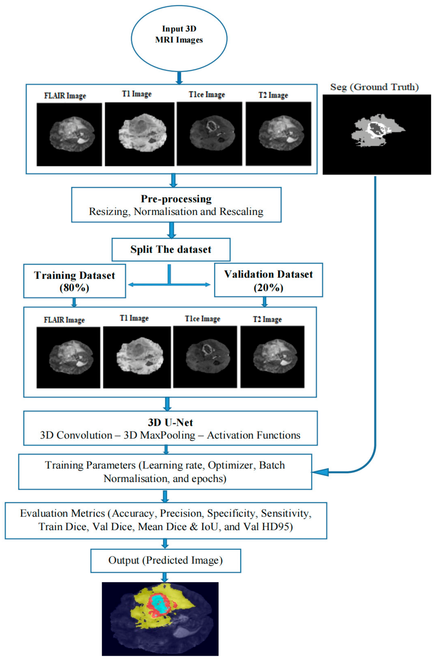
Figure 3 illustrates the systematic methodology: 1. Data preprocessing (resizing, rescaling and normalisation of input images); 2. dataset preparation (splitting of the BraTS dataset into training and validation); 3. model training (building the 3D U-Net architecture with chosen activation functions); and 4. evaluation metrics such as (accuracy, precision, specificity, DSC, Mean DSC, IoU, and HD95).

3.2. Building a 3D U-Net Model

An improved 3D U-Net architecture, hereafter referred to as ImprovedUNet3D, has been developed specifically for brain tumour segmentation in this study. Residual Blocks in the ImprovedUNet3D model improved gradient propagation and feature mapping across deep layers of the U-Net architecture. Each Residual Block includes two 3 × 3 × 3 convolutional operations with batch normalisation and activation functions and a shortcut connection defined as:
y   =   F ( x )   +   W S x ,
where F ( x ) signifies the primary transformation route, and W S x indicates the shortcut link. The shortcut connection will be established using a 1 × 1 × 1 convolution when the number of input and output channels is unequal. This guarantees that both dimensions are consistent before applying the element-wise summation.
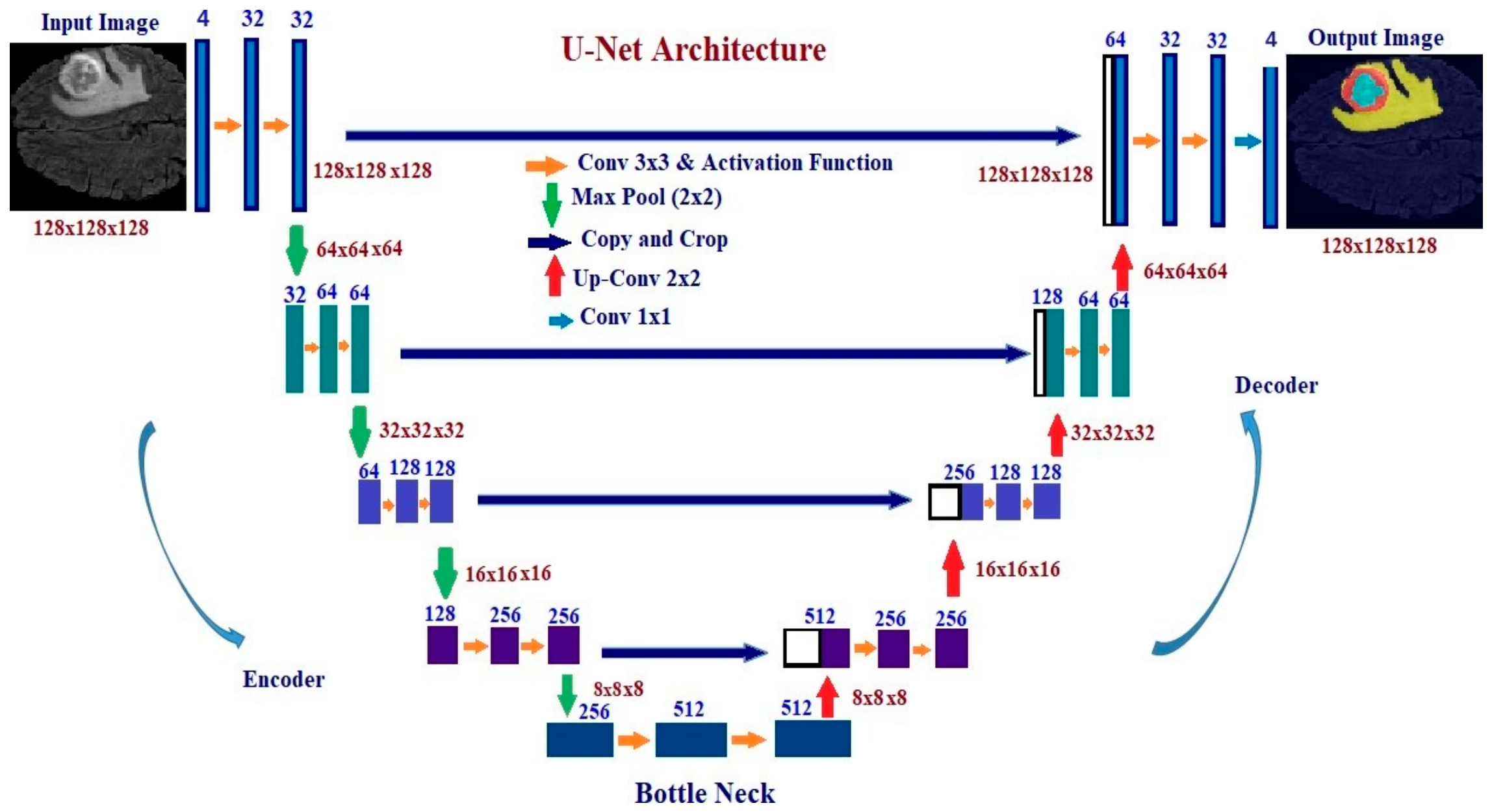
The structure consists of four levels with →32→64→128→256 channels in the encoder. Each level of the encoder consists of one Residual Block followed by 2 × 2 × 2 max pooling operations. At the encoder bottleneck, a Residual Block computes a 512-channel representation. The decoder is structured to maintain the same spatial resolution as the encoder via transposed convolutions, concatenated skip connections from the encoder, and Residual Blocks at each level, reducing channels from 512→256→128→64→32 A single 1 × 1 × 1 convolution operation finalises the decoding process by creating a single representation for the Cout segmentation classes that the model uses when applying Softmax in the loss function. Throughout the model’s development, the ImprovedUNet3D architecture demonstrated better feature extraction, improved optimisation stability, and higher volumetric accuracy in multimodal MRI image segmentation.

Architecture Specification

The core segmentation model utilised in this study is a lightweight, custom-designed 3D Residual U-Net (ImprovedUNet3D). The network comprises a 4-level encoder–decoder structure connected by a bottleneck layer. To mitigate the vanishing gradient problem in deep 3D networks, standard convolutional blocks were replaced with Residual Blocks. Each Residual Block consists of two consecutive 3 × 3 × 3 3D Convolutional layers, each followed by 3D batch normalisation and the specified experimental activation function (e.g., ReLU or Swish). A 1 × 1 × 1 3D Convolutional skip connection is added if the input and output channel dimensions differ. Downsampling is achieved via 2 × 2 × 2 Max Pooling, while upsampling utilises 2 × 2 × 2 3D Transposed Convolutions (stride 2). The final output layer is a 1 × 1 × 1 3D Convolution mapping to the 4 BraTS target classes. Table 2 shows a detailed layer-by-layer specification of the used 3D Residual U-Net. The total trainable parameter count for the network is exactly 22.93 million, ensuring a highly efficient memory footprint suitable for standard clinical hardware.
Figure 4 shows the proposed 3D U-Net model. The model takes an input image of size 128 × 128 × 128 and uses a symmetric encoder–decoder architecture. The convolutional layers in the encoder use 3 × 3 kernels to reduce the image’s spatial dimensions while extracting high-level features. In the encoder, max pooling with a 2 × 2 kernel is applied to further reduce the image size. The decoder then reconstructs the resolution of the upsampled image from the encoder using 2 × 2 up-convolution layers, concatenating each upsampled feature map with the encoder’s cropped feature map to maintain spatial detail in the final segmentation output generated by 1 × 1 convolutional layers.

3.3. Activation Functions

Non-linear activation functions play a significant role in constructing deep learning models for capturing heterogeneous morphological features in multimodal MRI scans. These functions transform the linear inputs into non-linear outputs to enable the network to learn and capture complex features, hierarchical representations necessary for accurate segmentation of tumour sub-regions. Furthermore, selecting an appropriate activation function is crucial in stabilising the training process of deep architectures, directly influencing computational efficiency and mitigating gradient-related degradation, like the vanishing gradient problem.
The choice of activation function is a determining factor in the network’s ability to model complex, nonlinear boundaries between tumour and healthy tissue. To this end, we designed an experimental framework that investigates twelve activation functions, categorised into two groups: traditional rectified units (ReLU) [23], Leaky ReLU [24], PReLU [25], ELU [27] and their modern smooth or self-gated variants: GELU [28], Swish [22], Mish [29], EliSH, HardELiSH [26], TanhExp [30], Logish [31], and Smish [32]. We specifically selected this diverse set to directly contrast the rigid, piecewise-linear behaviour of traditional rectifiers against the continuous, non-monotonic properties of modern self-gating functions. We train the model independently with each of them, with the goal of benchmarking their impact on gradient flow and generalisation capabilities and, particularly, of isolating the trade-offs between computational complexity and segmentation performance in MRI analysis.

3.3.1. Evaluation of Activation Function Strategy

To make fair and impartial comparisons between experiments, all experiments used the same Improved UNET3D network architecture, the same loss function, optimisation method and its parameters, mini-batch size, and the same preprocessing method for training and predicting images. The only difference across sets of experiments was the activation method applied to the convolutional blocks of their network architectures. By strictly freezing all other network parameters and data augmentation pipelines, this controlled environment allows for the direct evaluation of the effects of nonlinear activation functions on gradient flow, convergence, stability, and segmentation accuracy, without interference from changes in architecture or optimisation methods.

3.3.2. The Critical Role of Activation Functions

The work is driven by the hypothesis that optimising the core non-linearity of the U-Net will enable the direct tackling of ReLU shortcomings and improve sub-region segmentation accuracy. The activation function is the basic “decision-maker” in a neuron.
By implementing a Parametric ReLU (PReLU), we introduce a learnable parameter ( α ) that controls the response to negative inputs. This setup offers two benefits:
  • Inhibits Neuron Death: Setting the gradient for negative inputs to a non-zero, learnable value addresses the “dying ReLU” issue and ensures the network’s capacity to learn remains intact.
  • Increases Model Expressiveness: The learnable parameter enables the model to adapt to more complex data distributions, which is crucial for capturing subtle boundaries and the internal heterogeneity of brain tumour sub-regions.
Therefore, our work offers a more focused study of a core element used in deep segmentation networks. We therefore examine whether more flexible, adaptive functions such as PReLU—alongside smooth, self-gated functions—enhance sub-region segmentation, testing this empirically rather than assuming it.
Table 3 shows the formulas and characteristics of twelve activation functions utilised in this study.
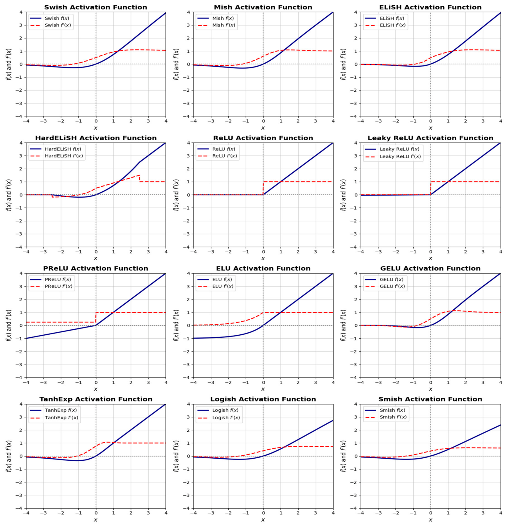
Figure 5 shows a graphical representation of the twelve activation functions explored in this study and their derivatives. The figure starts with the Swish activation function and ends with the Gaussian Error Linear Unit (GELU). Each of the twelve activation functions and its corresponding derivatives is explicitly shown in dedicated visualisations, produced programmatically in Python 3.12.13 using common scientific libraries within a Google Colab environment.
The pipeline was implemented in Python 3.12.13 using PyTorch 2.10.0, with NumPy 2.0.2, SciPy 1.16.3, nibabel 5.4.2, pandas 2.2.2 and Matplotlib 3.10.0/Seaborn 0.13.2 for data handling, metric computation and visualisation, and fvcore for FLOP analysis, within the Google Colab environment (runtime 2026.04), on NVIDIA A100-SXM4-40GB and NVIDIA L4 GPUs (NVIDIA Corporation, Santa Clara, CA, USA).

3.4. Experimental Setup and Training Details

To ensure absolute reproducibility and a strictly controlled environment for the activation-function ablation study, all network variants were trained under identical configurations.

3.4.1. Data Partitioning and Augmentation

The BraTS 2020 dataset (369 patient volumes) was partitioned into a training set (80%) and a hold-out validation set (20%). All MRI modalities (T1, T1ce, T2, FLAIR) were z-score intensity-normalised and centre-cropped to a 128 × 128 × 128 region during preprocessing (Section 3.1.5 and Section 3.1.6). To ensure that variations in performance were strictly attributable to the mathematical properties of the activation functions rather than stochastic data transformations, dynamic spatial data augmentations (e.g., random rotations or elastic deformations) were deliberately omitted during the training loop, establishing a pure, unconfounded baseline for activation behaviour.

3.4.2. Hyperparameters and Optimisation

All models were trained from scratch for exactly 100 epochs using a batch size of 2. Optimisation was performed using the AdamW optimiser with an initial learning rate of 3   ×   10 4 . To facilitate smooth convergence, the learning rate was modulated using a Cosine Annealing scheduler ( T m a x   =   100 ). The network weights were optimised using a combined loss function consisting of standard Cross-Entropy Loss and Soft Dice Loss, ensuring both pixel-wise classification accuracy and holistic volumetric overlap.

3.4.3. Hardware, Mixed Precision, and Reproducibility

Training was accelerated utilising PyTorch 2.10.0 Automatic Mixed Precision (AMP), which scales gradients via torch.amp.GradScaler to significantly reduce GPU memory consumption (VRAM) without degrading mathematical precision. To eliminate training variance and guarantee a fair head-to-head comparison, all experimental runs were initialised with a globally fixed random seed (seed = 42), enforcing deterministic behaviour across PyTorch, NumPy, and cuDNN backends. Therefore, the reported results represent single, highly controlled, deterministic runs rather than multi-trial averages. Convergence criteria dictated that the final model weights selected for inference were those that achieved the highest mean whole-tumour Dice score on the validation set during the 100-epoch training cycle.

3.5. Training Process

All model training and experiments were conducted using Google Colab Pro+ with an NVIDIA GPU (40 GB VRAM). The model was trained for 100 epochs using the AdamW optimiser, widely recognised for its stability and strong performance in deep learning applications, with an initial learning rate of 3 × 10 4 .
First, gradients are computed as follows:
g t   =     θ t   L ( θ t ) ,
Then update the rule for AdamW is defined as:
m t   =     β 1     m t 1   +   1     β 1 g t ,
v t = β 2     v t 1 + 1 β 2 g t 2 ,
v ^ t = max ( v ^ t 1 ,   v ^ t ) ,
θ t + 1 = θ t ղ v ^ t   + ϵ   m t ,
where m t , v t are the first and second biased moment estimates, respectively, v t is the bias-corrected counterpart, g t represents the gradient of the loss function, β 1 , β 2 are exponential decay rates for the first and second moment estimate (commonly set to 0.9 and 0.999). ϵ is a small constant (e.g., 10 8 ) to prevent division by zero, is the learning rate.
Learning Rate Schedule (Cosine Annealing): The learning rate, denoted by η(t), was controlled by a Cosine Annealing schedule. Cosine Annealing is a method of reducing the learning rate from a maximum value to a minimum value according to a cosine curve, sometimes with restarts or cyclical learning. For a given epoch ( t ), the learning rate η( t ) is calculated as:
η t =   η m i n   + 0.5 ( η m a x η m i n )     1 + cos t T m a x π
where η m a x is the initial maximum learning rate, η m i n is the minimum learning rate, t is the current epoch number (or iteration number) and T m a x is the total number of epochs (or maximum number of iterations for one cycle). In addition, Cosine Annealing learning rate is used as the scheduler, allowing aggressive learning in the early training phase and, as training progresses, finer adjustments, which may lead to better convergence and generalisation. The network was optimised with a combined loss consisting of an unweighted Cross-Entropy term and a soft-Dice term. Such a loss function allows the Cross-Entropy component to handle pixel-wise classification, while the Dice component directly optimises overlap between predicted and ground-truth segmentations, which is important for imbalanced medical image segmentation tasks.
No per-class Cross-Entropy weighting was applied; class imbalance is addressed by the Dice component, and the loss was kept identical across all activation-function experiments so that performance differences are attributable solely to the activation function. Finally, to accelerate the training process with a smaller memory footprint, the Automatic Mixed Precision (AMP) is enabled using torch.cuda.amp.GradScaler to allow training the model with lower precision when it is numerically safe to do so. Regular evaluation on a validation set was performed within the training loop, and the model state dictionary with the best validation loss was saved to disk, ensuring that the best-performing model was preserved. The code also performs garbage collection and clears the CUDA cache at the start of each new epoch to optimise memory usage, particularly for large 3D data.
A set of comprehensive evaluation metrics has been utilised to assess and evaluate the performance of the 3D U-Net architecture on this particular task. Overlap metrics—the Dice Similarity Coefficient and Jaccard Index [55,56] have been utilised to assess the degree of conformity between the segmentation outcome of the model and the ground-truth segmentations of the tumour sub-regions such as the necrotic core, oedema, and enhancing-tumour regions.
These metrics are very relevant to medical image segmentation, where the proper delineation of structures is essential. In addition to the above-mentioned overlap metrics, sensitivity, precision, and specificity are computed on a per-class basis. Sensitivity measures the model’s ability to identify all positive pixels, while precision is the number of correctly identified positive pixels divided by the total number of pixels predicted as positive. Specificity expresses the model’s ability to correctly identify negative pixels (true negatives) [56]. Furthermore, surface distance metrics such as the Hausdorff Distance 95 (HD95) provide a robust quantification of boundary accuracy [57] (outliers are handled) by computing the minimum Hausdorff Distance between the predicted and true segmentation boundaries. The HD95 is computed for each tumour sub-region after post-processing the predictions by removing small connected components (noise) to ensure that only biologically relevant segmentations contribute to the metric [58]. The intersection over Union (IoU) further quantifies the overlap between predicted and ground-truth regions [59].
Table 4 presents the comprehensive suite of metrics used to evaluate the model’s performance in this study. Each metric is mathematically derived on a per-class level and then averaged to provide an overall understanding of segmentation accuracy and quality. Collectively, these metrics offer a robust assessment of the model’s capabilities.

Statistical Reliability of the Results

All of these evaluation scores were calculated on a per-class basis over each validation volume, then averaged over the validation set. In an attempt to reduce the impact of outliers, in these results, the Hausdorff Distance was measured using the 95th percentile (HD95). While there were minor discrepancies among the various activation functions, clear trends were noticed across several supporting scores such as the Dice Score, IoU, sensitivity, and HD95.
Statistical analysis: For every metric and tumour sub-region, each activation function was compared against the ReLU baseline using the Wilcoxon signed-rank test, a non-parametric paired test. Pairing was performed per patient, matching the two models on the same validation volumes, so that each comparison reflects within-subject differences without assuming normally distributed scores—appropriate given the skewed Dice and heavy-tailed HD95 distributions. Significance is denoted in Table 5, Table 6, Table 7 and Table 8 as * (p < 0.05) and ** (p < 0.01). Because each activation × region × metric cell constitutes a separate test, we additionally report Holm- and Benjamini–Hochberg (BH)-adjusted p-values computed across the comparison family of each metric. The principal necrotic-core improvement of Swish over ReLU remains significant under both corrections (raw p < 0.001; Holm-adjusted p = 0.024; BH-adjusted p = 0.012), while several smaller single-run differences survive only the less conservative Benjamini–Hochberg control. The multi-seed and cross-validation analyses (Section 5.6) establish which of these single-run effects generalise; in particular, the enhancing-tumour and PReLU differences do not.

4. Results

4.1. Segmentation Accuracy: Dice Similarity and Hausdorff Distance

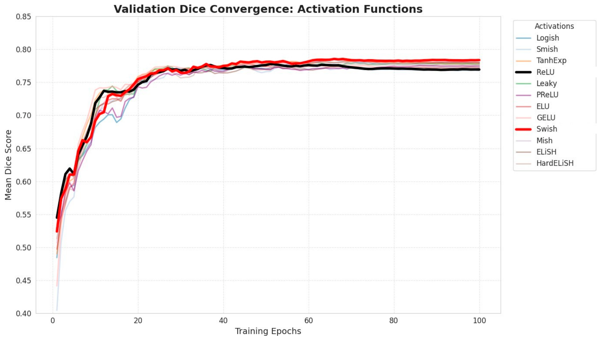
Quantitative evaluation reveals that smooth, non-monotonic activation functions consistently yield superior boundary delineation over standard rectified units. The learning curves for the 12 evaluated activation functions show rapid initial convergence within the first 20 epochs before reaching a stabilisation phase. As illustrated in Figure 6, while all models eventually converge to a high-performance plateau with a mean Dice score greater than 0.75, Swish (the winner) exhibits the most robust and stable performance throughout the latter half of the training process. Swish and TanhExp consistently outperformed the ReLU baseline in final mean Dice scores. Quantitative comparisons across tumour sub-regions are detailed in Table 5. The baseline ReLU achieved mean Dice scores of 0.805 for the enhancing tumour (ET) and 0.871 for the tumour core (TC). Swish demonstrated a statistically significant improvement (p < 0.01) over this baseline, achieving 0.812 for ET and 0.864 for TC.
Notably, while TanhExp emerged as the top performer for the whole-tumour (WT) region with a Dice score of 0.879, Swish consistently outperformed all other functions in the critical intratumoral structures (necrotic core and enhancing tumour). This suggests that while TanhExp is superior for volumetric delineation, Swish captures the fine-grained internal boundaries more effectively.
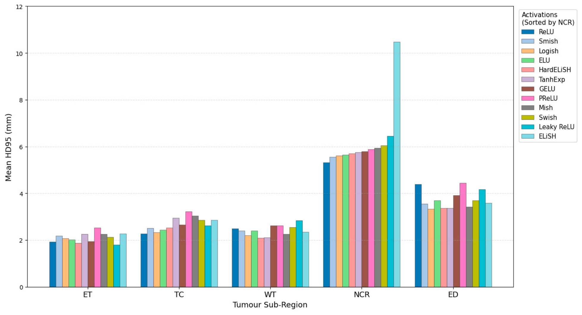
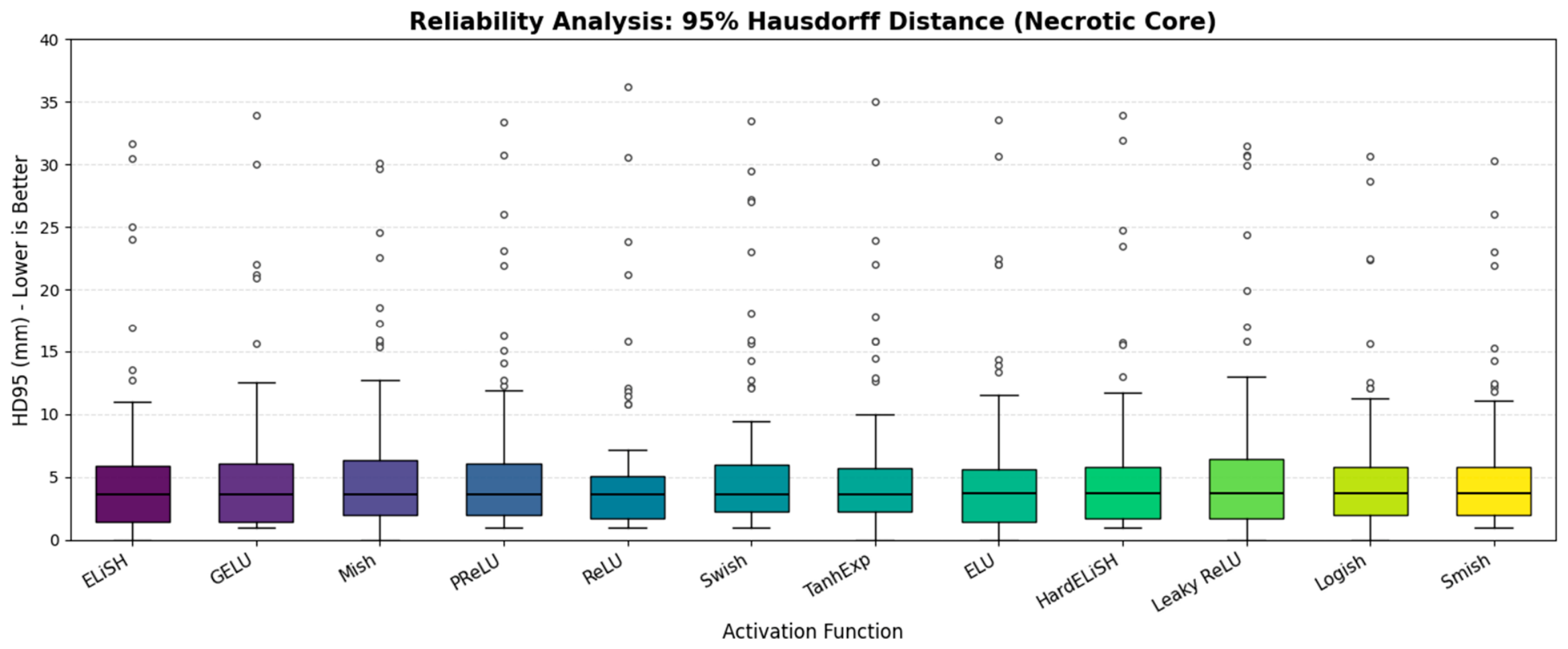
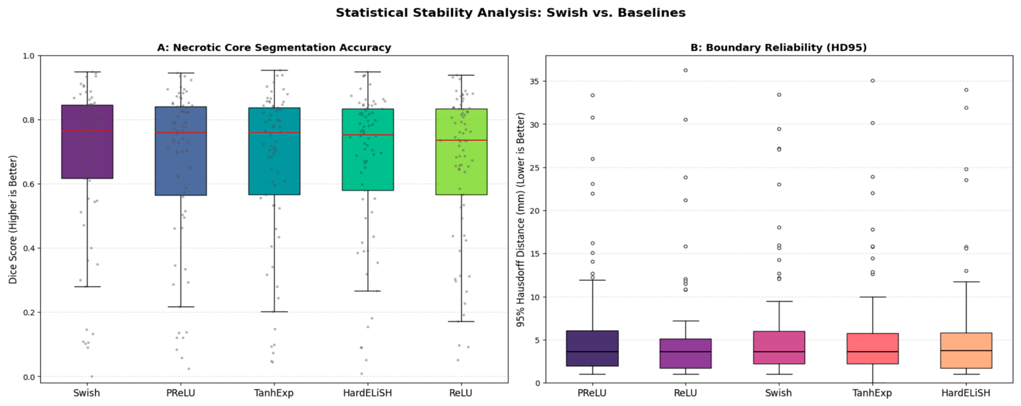
Regarding boundary delineation reliability, the 95% Hausdorff Distance (HD95) results (Table 6, Figure 7) demonstrate that Leaky ReLU achieved the highest stability in the enhancing-tumour region with the lowest mean HD95 of 1.79 mm. While Swish yielded a slightly higher mean HD95 (2.13 mm) than ReLU (1.93 mm), the difference was not statistically significant. Importantly, Swish avoided the catastrophic boundary instability seen in ELiSH, which produced extreme outliers in the necrotic core (HD95 10.48 ± 43.49 mm, reflecting occasional empty predictions); the remaining functions, including HardELiSH, were far more contained. This reliability in the necrotic core is further visualised in the boxplots (Figure 8), where significant outliers (up to 35 mm) highlight the boundary instability of certain functions despite low median values.
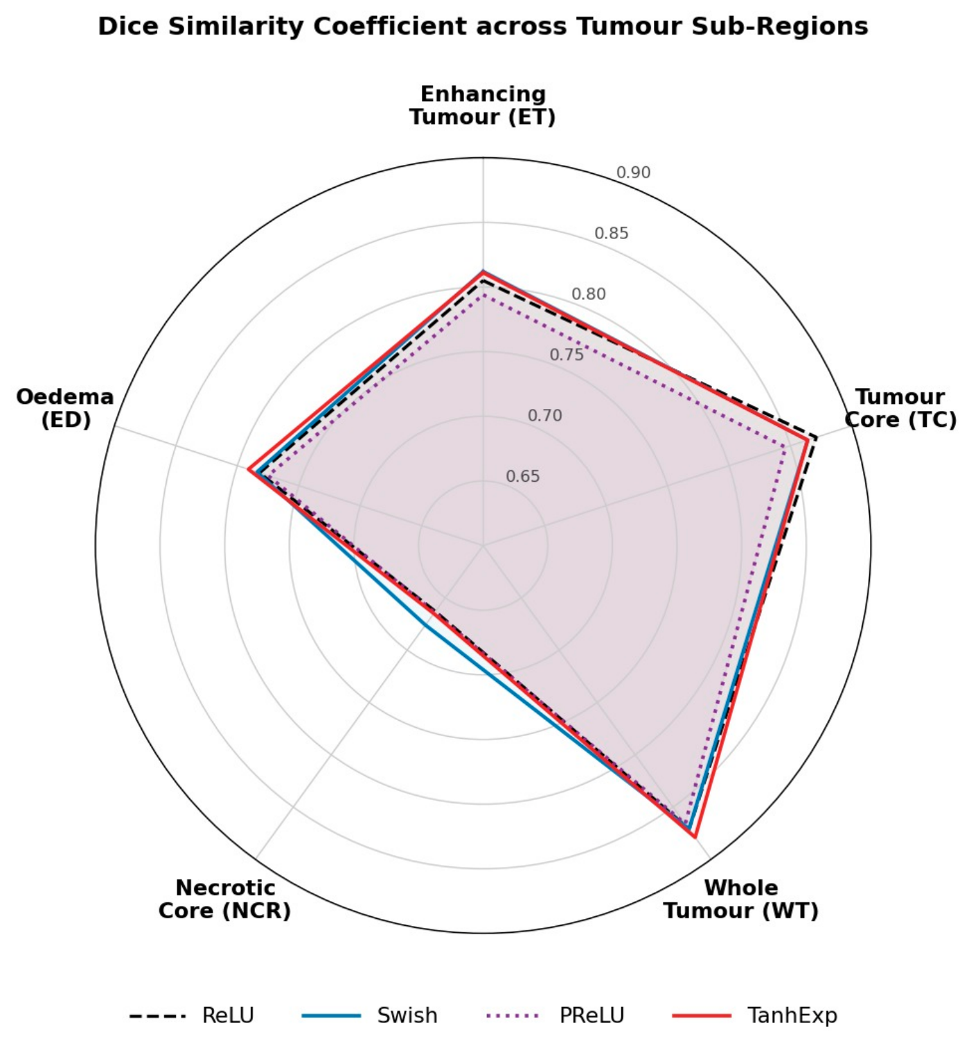
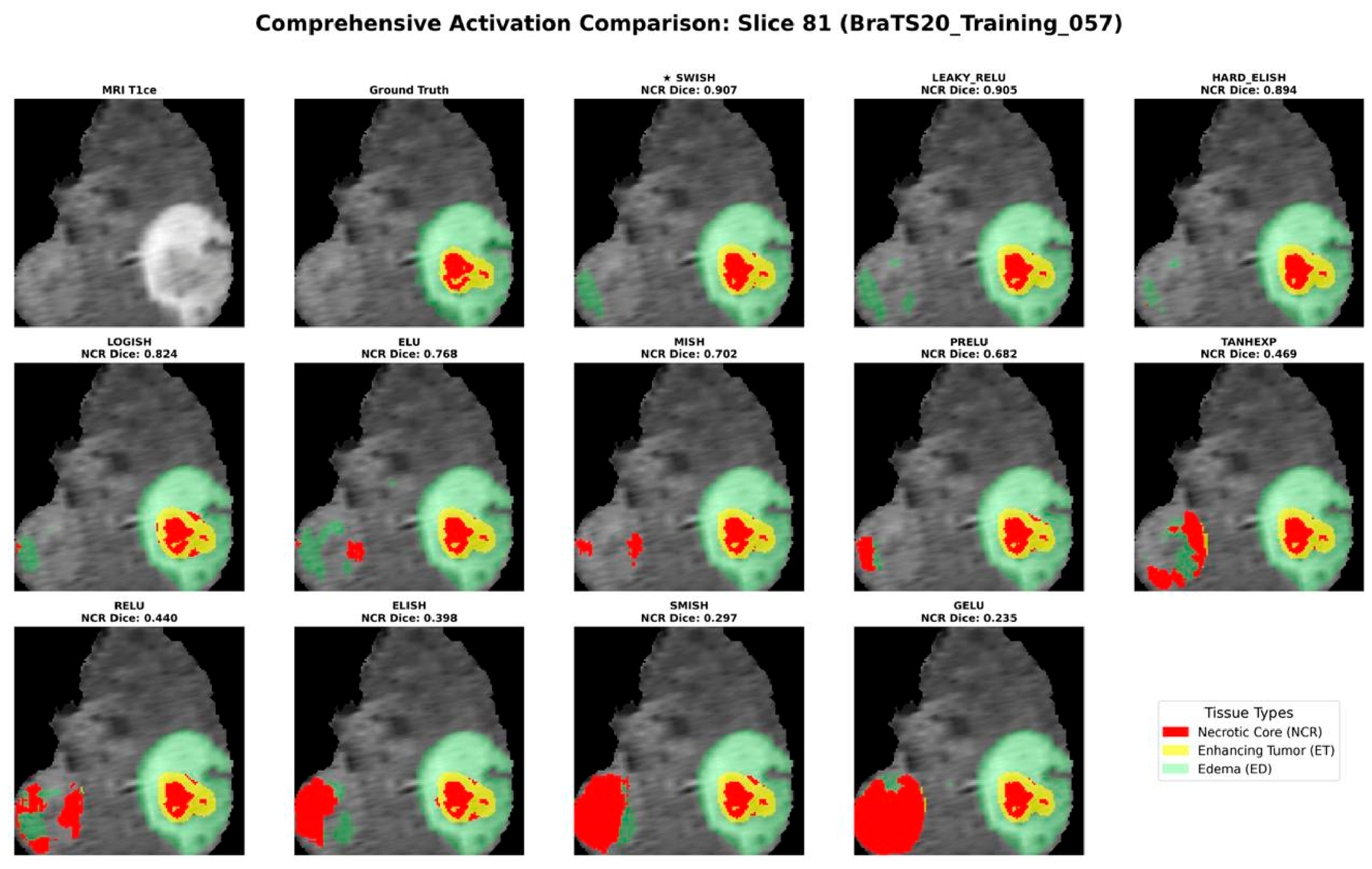
A holistic view of performance is provided in the radar chart (Figure 9) comparing Dice Similarity Coefficients (DSCs) across five sub-regions. While TanhExp shows a marginal lead in the whole tumour and ReLU remains highly competitive in the tumour core, the differences between functions are small across all regions. Qualitative results further support these findings, showing that while most functions capture the primary mass, variations in necrotic-core Dice scores (0.235 to 0.907) highlight differences in local boundary precision.

4.2. Qualitative Analysis of Segmentation Boundaries

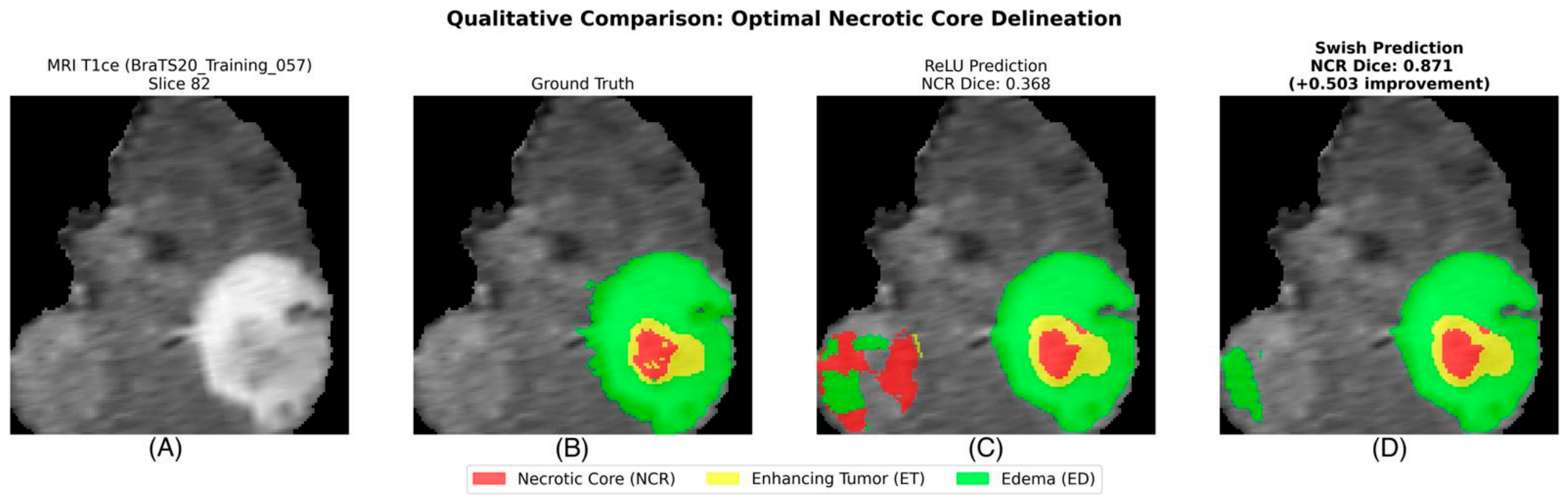
To validate these quantitative improvements, we examined segmentation quality on challenging validation cases (Figure 10). Specifically, Figure 11 presents a comparative overlay for Patient BraTS20_Training_057 (Slice 82), a case characterised by a highly complex, jagged necrotic-core boundary. To better illustrate the morphological differences captured by the 95% Hausdorff Distance (HD95) metric, magnified insets are provided for the region of interest.
The baseline ReLU model exhibits characteristic over-smoothing, failing to preserve the intricate internal topology of the necrotic core (Slice NCR Dice: 0.368). In contrast, the Swish model successfully delineates the complex, fragmented boundary of the necrotic core with high fidelity (Slice NCR Dice: 0.871), achieving a morphological structure significantly closer to the ground truth.

4.3. Sensitivity and Precision Analysis: The “Aggression” Trade-Off

To identify the drivers of performance, sensitivity (recall) and precision (PPV) were analysed (Table 7 and Table 8). This granular analysis exposes a critical tension between volume overestimation and boundary precision. ReLU exhibited the highest sensitivity (ET: 0.857, TC: 0.882), but at the cost of significantly lower precision (ET: 0.777), suggesting a tendency to over-segment. Conversely, Swish acted as a more discriminative filter; although its enhancing-tumour sensitivity was lower than ReLU (0.818 vs. 0.857), its precision was 5.0% higher (0.827).

4.4. Statistical Stability and Outlier Analysis

Beyond mean accuracy, clinical reliability requires consistent performance across the entire patient population. The distribution of Dice scores and Hausdorff Distances (HD95) for the necrotic-core highlights important differences in stability across activation functions (Figure 12).
While the baseline ReLU shows a reasonable median performance, it exhibits a wider interquartile range (IQR) and several significant outliers, indicating inconsistent performance on difficult cases. ELiSH displays the most extreme instability, its necrotic-core HD95 reaching the empty-prediction penalty (mean 10.48 ± 43.49 mm), which renders it unsuitable for clinical automation; the remaining functions, including HardELiSH, show far more contained HD95 distributions. Swish combines a higher median necrotic-core Dice with the tightest interquartile range among the evaluated functions, indicating consistent central performance, although its HD95 distribution is comparable to that of the other functions rather than uniquely free of outliers.

4.5. Computational Efficiency and Resource Utilisation

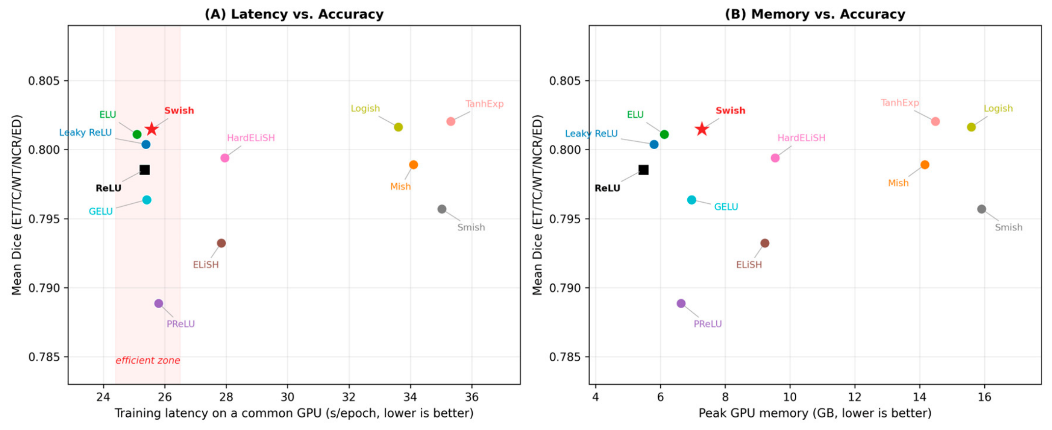
To enable a fair comparison, all twelve activation functions were profiled on a single common GPU (NVIDIA A100-SXM4-40 GB; full results in Supplementary Table S2), removing the need for any cross-hardware normalisation. On this common hardware, the simple rectified units (ReLU, Leaky ReLU, ELU) and Swish were the fastest at approximately 25 s per epoch, while the complex functions Logish, Mish, Smish and TanhExp were the slowest at 33–35 s per epoch (1.33–1.39× the ReLU baseline). For instance, Mish required about 1.35× the per-epoch time of ReLU—substantial, but well below the threefold figure suggested by the earlier cross-hardware normalisation.
Swish occupies the optimal efficiency–accuracy zone: on common hardware it introduces only a ~1% latency penalty (25.6 s vs. 25.3 s per epoch) over ReLU while delivering its necrotic-core accuracy gain. The piecewise HardELiSH increased per-epoch time by only about 10% (28.0 s)—not the very large penalty implied by the earlier normalised figures—whereas the smooth, exponential-based functions (Mish, Logish, Smish, TanhExp) carried the largest cost, in both latency (~1.35×) and peak memory.
From an architectural efficiency perspective, Swish occupies the Pareto-optimal frontier (Figure 13). It achieves top-tier accuracy with a training latency comparable to ReLU, whereas complex functions such as TanhExp and Logish were 33–39% slower on common hardware. While memory usage was largely dominated by the U-Net backbone, Mish and TanhExp showed a measurable increase in peak VRAM due to more complex gradient storage requirements.

5. Discussion

5.1. The Precision–Sensitivity Trade-Off: Scalpel vs. Blunt Instrument

Our comprehensive evaluation reveals a fundamental dichotomy in activation-function behaviour for medical image segmentation, highlighting that raw sensitivity does not necessarily equate to clinical utility. The baseline ReLU function demonstrated the highest sensitivity (recall) across the enhancing-tumour (ET: 0.857) and tumour-core (TC: 0.882) regions. However, this high sensitivity was accompanied by significantly lower precision (ET: 0.777), indicating a tendency toward systemic over-segmentation. In clinical terms, ReLU behaves as a “blunt instrument,” capturing the majority of true tumour voxels but failing to discriminate them effectively from surrounding oedema or healthy tissue.
In contrast, Swish emerged as a “precision instrument.” While it sacrificed moderate sensitivity (~4%), this trade-off was justified by a significant improvement in precision (+5.0% in ET compared to ReLU). This suggests that Swish’s non-monotonic and smooth profile enables the network to learn more complex, discriminative features, resulting in segmentation boundaries that are sharper and more clinically reliable than the baseline. This finding challenges the conventional reliance on ReLU for medical segmentation, proposing that precision (i.e., reduction in false positives) is a critical driver of improved Dice performance in modern architectures.
This precision is visually corroborated by the magnified qualitative analysis (Figure 11), which demonstrates Swish’s ability to faithfully trace jagged, non-linear tumour concavities that the ReLU baseline blindly over-smooths.

5.2. Necrotic-Core Trade-Offs and Learnable Activations

The necrotic core (NCR) represents the most challenging sub-region due to its irregular shape and textural similarity to the surrounding tumour core. HardELiSH achieved the highest precision (0.835), demonstrating exceptional selectivity. However, its low sensitivity (0.602) renders it overly conservative for clinical safety. Swish provided the optimal balance, improving NCR Dice scores to 0.676 (p < 0.01) by filtering background noise without aggressively discarding true positive voxels. In practical terms, the necrotic core is a marker of tumour aggressiveness and treatment response, so a more faithful delineation of its irregular boundary supports more consistent volumetric tracking over time; nevertheless, this ~2% absolute Dice gain is best interpreted as an incremental, zero-cost reliability improvement that is unlikely on its own to alter an individual clinical decision.
In the single-seed run, the learnable PReLU function appeared not to improve performance, showing reduced enhancing-tumour sensitivity (0.789 vs. ReLU’s 0.857, a relative drop of 6.8%). However, our three-seed reliability analysis (Section 5.6) showed that this underperformance did not generalise: averaged across seeds, PReLU was competitive in every sub-region and matched Swish on the necrotic core (0.678 vs. 0.677). The single-run weakness therefore appears to have been largely seed-driven rather than an intrinsic limitation of the learnable activation, and we caution against over-interpreting single-seed differences between closely matched functions.

5.3. Computational Cost and Efficiency Analysis

A critical factor in deploying 3D medical imaging models to clinical environments is their computational footprint. To substantiate the cost-effectiveness of substituting the standard ReLU activation with Swish, we profiled the architectural and computational overhead of both models during training and inference (Table 9).
f ( x ) = x σ ( x ) where σ ( x ) is the logistic sigmoid activation function.
Because Swish () is a mathematical substitution applied element-wise, it introduces exactly zero additional trainable parameters to the 22.93 M parameter network. As tracked by the fvcore hardware profiler, the floating-point operations (FLOPs) remained identical at 491.28 GFLOPs, as the addition of a sigmoid multiplication is highly optimised on modern hardware and completely dwarfed by the cost of the 3D convolutions. During our mixed-precision training loop, peak GPU memory utilisation (VRAM) for Swish saw only a marginal increase (+1.16 GB; 6.96 GB versus 5.80 GB for ReLU) due to the caching of intermediate tensors required for backpropagation, remaining well within the capacity of standard GPUs. Training time per epoch was virtually identical (25.6 s versus 25.3 s on a common A100 GPU, a ~1% difference). Furthermore, the inference time required to process a full 128 × 128 × 128 3D MRI volume was comparable (~28 ms for both functions, the cost being dominated by the 3D convolutions rather than the activation). These metrics quantitatively verify that the significant +2.0% Dice improvement in necrotic-core segmentation achieved by Swish comes at a negligible computational cost, confirming it as a highly cost-effective architectural upgrade.

5.4. Computational Efficiency on Common Hardware

Because the original profiling combined two different GPUs, we re-measured the per-epoch training time, inference time and peak memory for all twelve functions on a single GPU (NVIDIA A100-SXM4-40 GB), so that no cross-hardware normalisation is required (Supplementary Table S2). On common hardware, the complex functions TanhExp and Logish were 33–39% slower per epoch than Swish—a real but moderate overhead; the previously reported ~3.0× normalisation factor overstated this gap.
Swish demonstrated Pareto-optimal efficiency, achieving top-tier accuracy at near-baseline latency and memory. In contrast, Mish and TanhExp incurred a higher memory footprint due to the storage of intermediate tensors required for complex derivative computations. Consequently, while TanhExp may be suitable for offline processing scenarios where maximal accuracy is prioritised (e.g., tumour volume estimation), Swish remains the more practical choice in resource-constrained settings, where computational and real-time-inference constraints are critical considerations.

5.5. Performance Context and Architectural Benchmarking

To validate the reliability of our experimental framework, we compared our results against established benchmarks for the 3D U-Net architecture (Table 10). Our baseline ReLU model achieved an enhancing-tumour Dice score of 0.805, which compares favourably with published results for standard 3D U-Nets, including the attention-gated U-Net [60] (ET 0.760 on BraTS 2019, as reported in the TransBTS study [52]) and the hybrid CNN–Transformer TransBTS [52] (ET 0.787, WT 0.901 on BraTS 2020). This confirms that our implementation provides a robust baseline for isolating the effects of activation functions.
Notably, our best-performing model, Swish, achieved an enhancing-tumour Dice score of 0.812. This result surpasses standard U-Net benchmarks and approaches the performance of more complex architectures. The Swish model effectively matches the tumour-core performance of the BraTS 2020-winning nnU-Net framework (0.864 vs. 0.851 [47]) and is competitive with attention-gated U-Net variants [60], despite using a single lightweight network rather than the self-configuring, augmentation-heavy nnU-Net pipeline.
It is critical to contextualise the absolute Dice scores reported in this study—particularly for the challenging necrotic core (0.676)—against the broader landscape of BraTS 2020 challenge submissions. State-of-the-art (SOTA) frameworks, most notably the top-ranking nnU-Net variations, achieve substantially higher absolute segmentation accuracy (often creating a ~20% performance gap in specific sub-regions). However, these peak performances are overwhelmingly driven by heavy model ensembling, multi-stage cascading architectures, extensive test-time augmentations (TTA), and dynamic pipeline self-configurations. More recent Transformer-based architectures push these absolute scores higher still: Swin UNETR reports WT/TC/ET Dice of 0.926/0.885/0.858 on the larger BraTS 2021 cohort [51], while UNETR [53] has not been benchmarked on BraTS (its published brain tumour results use the Medical Segmentation Decathlon task) and is therefore discussed qualitatively rather than tabulated.
The primary objective of this research is not to establish a new SOTA absolute performance metric—which is often driven by computationally expensive ensemble heuristics rather than core architectural efficiency—but rather to conduct a strictly controlled ablation study isolating the specific impact of non-monotonic activation functions. To achieve this, we deliberately utilised a fixed, lightweight, single-stage 3D Residual U-Net. Comparing this parameter-efficient baseline directly against challenge-winning ensembles would conflate the benefits of massive architectural complexity with the intrinsic mathematical properties of the activation functions. By freezing the architectural capacity and training pipeline, our framework provides an unconfounded environment. This controlled setting conclusively demonstrates that merely substituting the standard ReLU with Swish yields a statistically significant (+2.0%, p < 0.01) improvement in necrotic-core segmentation. Thus, while our absolute baseline is lower than heavily engineered ensembles, the relative gains demonstrated by non-monotonic functions represent a fundamental, zero-cost architectural upgrade that can be seamlessly integrated into future SOTA pipelines to bridge this performance gap.

5.6. Reliability of the Key Findings: Multi-Seed and Cross-Validation

To assess the reliability of the single-seed results, the four functions central to our claims—ReLU, Swish, PReLU and TanhExp—were retrained under three independent random seeds (42, 1337 and 2025) with an otherwise identical pipeline, and evaluated on the same 73-patient validation set (Table 11; full per-metric results in Supplementary Table S1). Two findings were robust to seed. First, the necrotic-core advantage of the smooth and adaptive functions over ReLU reproduced: Swish (0.677 ± 0.003) and PReLU (0.678 ± 0.004) both exceeded ReLU (0.661 ± 0.012), with a pooled Wilcoxon signed-rank p < 0.001 across all 219 patient–seed pairs. Second, ReLU was the least stable function in this region (seed-level standard deviation 0.012 versus 0.003–0.004 for the smooth functions). By contrast, the differences between functions in the enhancing tumour, tumour core, whole tumour and oedema were small and fell within seed-level variability, and the single-run underperformance of PReLU was not reproduced. Notably, seed 42—the seed used for the main single-run tables—proved to be an outlier in which the Swish and PReLU necrotic-core advantages were not individually significant (p = 0.76 and p = 0.53), whereas both reached p < 0.001 under seeds 1337 and 2025. This directly motivates the multi-seed protocol requested during review.
To assess sensitivity to the particular data split, we additionally performed five-fold cross-validation over all 369 patient volumes for the same four functions, with the seed held fixed so that only the partition varied; each patient is scored once, by a model that never saw it (out-of-fold prediction; Table 12; full per-metric results in Supplementary Table S3). Because this evaluates the entire cohort rather than the single 73-patient hold-out set, the absolute Dice values differ from Table 5, Table 6, Table 7 and Table 8 (whole-tumour Dice is higher and enhancing-tumour Dice lower over the full cohort); the between-function comparison is the quantity of interest. The cross-validation reinforced the multi-seed findings. The necrotic-core advantage of Swish over ReLU was directionally consistent in every one of the five folds (+0.7 to +1.1 Dice points; mean +0.8), confirming that it is not an artefact of the chosen split, although the pooled difference across all 369 patients was small and did not reach significance (Wilcoxon p = 0.13). In the enhancing tumour, tumour core, whole tumour and oedema the functions were statistically indistinguishable, as before. Taken together, the multi-seed and cross-validation analyses indicate that activation-function effects in this task are small, region-specific (concentrated in the necrotic core) and consistent in direction, rather than large or broadly significant.

5.7. Mechanistic Analysis of Gradient Flow in Hypointense Regions

The empirical superiority of the Swish activation function ( f ( x ) =   x σ ( x ) ) over the baseline ReLU ( f x =   max 0 , x ) in segmenting the necrotic core (NCR) can be directly attributed to its non-monotonicity and gradient preservation properties in negative domains.
In multimodal MRI, the necrotic core typically presents as a highly hypointense (dark) region, particularly on T1-weighted contrast-enhanced (T1ce) sequences. Following standard zero-mean, unit-variance dataset normalisation, these low-intensity necrotic voxels frequently map to negative input values during forward propagation. Because the neural network processes these dark biological tissues as negative numerical values, the activation function’s mathematical treatment of the negative domain becomes the defining factor in segmentation success. When utilising ReLU, any negative pre-activation value is strictly clamped to zero. This hard thresholding introduces two critical failure modes for dark tissue: (1) Feature erasure in the forward pass, where subtle texture variations within the dead necrotic tissue are uniformly squashed to zero, making it impossible for deeper layers to distinguish boundaries; and (2) gradient zeroing (the “dying ReLU” phenomenon) during backpropagation. Because the derivative of ReLU is exactly zero for negative inputs, the network halts weight updates for these regions, failing to learn subtle morphological boundaries.
Conversely, Swish permits a bounded, non-zero negative output for negative inputs. This smooth, non-monotonic curve preserves the continuous relative differences between adjacent hypointense voxels in the forward pass, allowing the network to retain fine-grained textural information. Crucially, the derivative of Swish remains non-zero for negative inputs, facilitating continuous, stable gradient flow during backpropagation. This mechanistic advantage ensures that the network actively updates its weights in response to the subtle gradient shifts at the boundary of dead tissue, directly explaining the significant +2.0% Dice improvement observed in NCR segmentation.

5.8. Limitations

This study evaluated activation functions without data augmentation in order to isolate their effects, so the reported performance may underestimate the accuracy achievable under augmented training. Evaluation was limited to the BraTS 2020 dataset, without external, multi-institutional or prospective validation and without expert radiological assessment of the outputs, making the results a controlled benchmark rather than evidence of clinical applicability. In addition, the study employed a lightweight 3D Residual U-Net, and findings may differ for more advanced architectures such as UNETR and Swin UNETR. Nevertheless, the three-seed experiments and five-fold cross-validation supported the reproducibility of the key findings, particularly for necrotic-core segmentation, where Swish’s advantage over ReLU was consistent in direction across all seeds and folds.

6. Conclusions

This study presents a comprehensive benchmark of 12 activation functions for 3D brain tumour segmentation, extending beyond conventional accuracy metrics to include sensitivity, precision, boundary reliability, and computational efficiency. Our findings lead to three principal conclusions.

6.1. Swish Is a Stable, Low-Cost Choice for Necrotic-Core Segmentation

Swish consistently outperformed the industry-standard ReLU in Dice score and precision, particularly in the challenging necrotic core (+2.0%). While TanhExp demonstrated superior performance for total tumour volume delineation, Swish offered the best balance between boundary precision and computational efficiency. By effectively preserving subtle gradients in hypointense regions, this makes it a suitable choice for capturing heterogeneous intra-tumour structures, warranting further clinical validation.

6.2. Single-Seed Differences Must Be Interpreted with Care

Our three-seed reliability analysis (Section 5.6) tempers one of the single-run observations. Although PReLU appeared to underperform in the initial single-seed experiment, this did not reproduce: averaged over three seeds, PReLU was competitive across all sub-regions and matched Swish on the necrotic core. Rather than showing that learnable activations fail in imbalanced tasks, the data show that differences between closely matched activation functions can be smaller than the run-to-run variability of a single training seed. This reinforces the value of multi-seed evaluation and motivates caution when ranking activation functions from a single run.

6.3. Efficiency Remains a Critical Consideration

On common hardware, Swish offers the most favourable trade-off between segmentation quality and training latency. Its minimal computational overhead, combined with statistically significant accuracy gains, makes it the most practical candidate among the evaluated functions for resource-constrained research and pre-clinical settings. Ultimately, replacing ReLU with Swish is a zero-cost intervention that narrows the gap between theoretical accuracy and practical, resource-constrained medical-imaging research, though clinical adoption will require further validation.

7. Future Work

Future research should explore hybrid activation landscapes in which functions are dynamically selected based on feature context. For example, a spatially adaptive architecture could leverage the high sensitivity of ReLU for initial tumour localisation while transitioning to the high-precision Swish function for fine-grained boundary delineation. Such a mechanism could potentially mitigate the sensitivity–precision trade-off identified in this study and further advance the robustness of automated medical image segmentation systems.
Additionally, evaluating activation behaviour within emerging architectures—such as Transformer-based segmentation models—and validating results across multi-institutional datasets would further strengthen the generalisability and clinical relevance of these findings.

Supplementary Materials

The following supporting information can be downloaded at https://www.mdpi.com/article/10.3390/informatics13070118/s1, Table S1: Multi-seed reliability—across-seed Dice, sensitivity, precision and HD95 over three random seeds; Table S2: Same-hardware computational efficiency (per-epoch time, inference time and peak VRAM) for all twelve activation functions on a single NVIDIA A100-SXM4-40 GB GPU; Table S3: Five-fold cross-validation—across-fold Dice, sensitivity, precision and HD95.

Author Contributions

Conceptualisation, M.M.S. and E.M.H.; methodology, M.M.S.; software, M.M.S. and M.A.A.A.; validation, M.M.S. and M.A.A.A.; formal analysis, M.M.S. and M.A.A.A.; investigation, M.M.S.; resources, M.M.S., E.M.H. and M.E.S.; data curation, M.M.S.; writing—original draft preparation, M.M.S.; writing—review and editing, M.M.S., E.M.H., M.E.S. and M.A.A.A.; visualisation, M.M.S. and M.A.A.A.; supervision, E.M.H. and M.E.S.; project administration, E.M.H. All authors have read and agreed to the published version of the manuscript.

Funding

This research was supported by a scholarship from the Yemen–Sudan Cultural Exchange Programme, sponsored by the Ministry of Higher Education and Scientific Research of Yemen and the Ministry of Higher Education and Scientific Research of Sudan. The article processing charge (APC) was funded by Gamal Qaed Abdo Ahmed Al-Kamil.

Institutional Review Board Statement

Ethical review and approval were waived for this study because it exclusively utilised the publicly available, fully anonymised brain tumour segmentation (BraTS) datasets. As this research involves secondary computational analysis of previously de-identified data and no new human subjects were recruited or experimented upon by the authors, it is exempt from standard Institutional Review Board (IRB) requirements.

Informed Consent Statement

Not applicable. This study exclusively utilised the publicly available, fully de-identified BraTS 2020 dataset. As no new human subjects were recruited and all data was previously anonymised by the dataset providers, additional informed consent was not required.

Data Availability Statement

The multimodal MRI data analysed in this study are derived from the publicly available brain tumour segmentation (BraTS) 2020 dataset. This dataset can be accessed via the official BraTS challenge repository provided by the Centre for Biomedical Image Computing and Analytics (CBICA) at the University of Pennsylvania. The custom PyTorch scripts and model checkpoints supporting the findings of this study are available from the corresponding author upon reasonable request.

Acknowledgments

The authors thank Sudan University of Science and Technology for its institutional support and the organisers of the BraTS 2020 challenge for providing the dataset used in this study. During the preparation of this manuscript, the authors used Google Gemini 3.1 Pro to refine the academic language and structure; the authors have reviewed and edited the output and take full responsibility for the content of this publication.

Conflicts of Interest

The authors declare no conflicts of interest. The funders had no role in the design of the study; in the collection, analyses, or interpretation of data; in the writing of the manuscript; or in the decision to publish the results.

Abbreviations

The following abbreviations are used in this manuscript:
AMPAutomatic Mixed Precision
BraTSBrain Tumour Segmentation
CBICACentre for Biomedical Image Computing and Analytics
CNNConvolutional Neural Network
DLDeep Learning
DSCDice Similarity Coefficient
EDOedema
ETEnhancing Tumour
FLAIRFluid-Attenuated Inversion Recovery
FLOPsFloating Point Operations
GPUGraphics Processing Unit
MICCAIMedical Image Computing and Computer Assisted Intervention
MLMachine Learning
MRIMagnetic Resonance Imaging
NCRNecrotic Core
PPVPositive Predictive Value (Precision)
ReLURectified Linear Unit
ROIRegion of Interest
SOTAState-of-the-Art
T1ceT1-weighted contrast-enhanced
TTATest-Time Augmentation
VAEVariational Autoencoder
VRAMVideo Random Access Memory
WHOWorld Health Organisation
WTWhole Tumour

References

  1. American Cancer Society. Types of Brain Tumors and Spinal Cord Tumors in Adults. Available online: https://www.cancer.org/cancer/types/brain-spinal-cord-tumors-adults/about/types-of-brain-tumors.html (accessed on 17 August 2025).
  2. Hanif, F.; Muzaffar, K.; Perveen, K.; Malhi, S.M.; Simjee, S.U. Glioblastoma Multiforme: A Review of its Epidemiology and Pathogenesis through Clinical Presentation and Treatment. Asian Pac. J. Cancer Prev. 2017, 18, 3. [Google Scholar] [CrossRef] [Scilit] [PubMed]
  3. Louis, D.N.; Perry, A.; Wesseling, P.; Brat, D.J.; Cree, I.A.; Figarella-Branger, D.; Hawkins, C.; Ng, H.K.; Pfister, S.M.; Reifenberger, G.; et al. The 2021 WHO classification of tumors of the central nervous system: A summary. Neuro Oncol. 2021, 23, 1231–1251. [Google Scholar] [CrossRef] [Scilit] [PubMed]
  4. Glioblastoma|Treatment and Prognosis|Brain Tumour Research. Available online: https://braintumourresearch.org/pages/types-of-brain-tumours-glioblastoma?srsltid=AfmBOoqBc2DtXCpMfVxzW5UicUeL4uTbt8TcvKC94iJr-sYXktHE8fcG (accessed on 2 March 2026).
  5. Sabeghi, P.; Zarand, P.; Zargham, S.; Golestany, B.; Shariat, A.; Chang, M.; Yang, E.; Rajagopalan, P.; Phung, D.C.; Gholamrezanezhad, A. Advances in Neuro-Oncological Imaging: An Update on Diagnostic Approach to Brain Tumors. Cancers 2024, 16, 576. [Google Scholar] [CrossRef] [Scilit] [PubMed]
  6. Bakas, S.; Zeng, K.; Sotiras, A.; Rathore, S.; Akbari, H.; Gaonkar, B.; Rozycki, M.; Pati, S.; Davatzikos, C. GLISTRboost: Combining multimodal MRI segmentation, registration, and biophysical tumor growth modeling with gradient boosting machines for glioma segmentation. In Brainlesion: Glioma, Multiple Sclerosis, Stroke and Traumatic Brain Injuries; Lecture Notes in Computer Science; Springer International Publishing: Cham, Switzerland, 2016; Volume 9556, pp. 144–155. [Google Scholar]
  7. Saleh, M.M.; Salih, M.E.; Ahmed, M.A.A.; Hussein, A.M. From Traditional Methods to 3D U-Net: A Comprehensive Review of Brain Tumour Segmentation Techniques. J. Biomed. Sci. Eng. 2025, 18, 1–32. [Google Scholar] [CrossRef]
  8. Khilkhal, R.; Ismael, M. Brain Tumor Segmentation Utilizing Thresholding and K-Means Clustering. In Proceedings of the Al-Muthanna 2nd International Conference on Engineering Science and Technology (MICEST 2022); IEEE: New York, NY, USA, 2022; pp. 43–48. [Google Scholar]
  9. Hasan, S.M.K.; Ahmad, M. Two-step verification of brain tumor segmentation using watershed-matching algorithm. Brain Inform. 2018, 5, 8. [Google Scholar] [CrossRef] [Scilit] [PubMed]
  10. Verma, O.P.; Hanmandlu, M.; Susan, S.; Kulkarni, M.; Jain, P.K. A simple single seeded region growing algorithm for color image segmentation using adaptive thresholding. In Proceedings of the 2011 International Conference on Communication Systems and Network Technologies (CSNT 2011); IEEE: New York, NY, USA, 2011; pp. 500–503. [Google Scholar]
  11. Aslam, A.; Khan, E.; Beg, M.M.S. Improved Edge Detection Algorithm for Brain Tumor Segmentation. Procedia Comput. Sci. 2015, 58, 430–437. [Google Scholar] [CrossRef] [Scilit]
  12. Abdel-Maksoud, E.; Elmogy, M.; Al-Awadi, R. Brain tumor segmentation based on a hybrid clustering technique. Egypt. Inform. J. 2015, 16, 71–81. [Google Scholar] [CrossRef] [Scilit]
  13. Krizhevsky, A.; Sutskever, I.; Hinton, G.E. ImageNet Classification with Deep Convolutional Neural Networks. Adv. Neural Inf. Process. Syst. 2012, 60, 84–90. [Google Scholar] [CrossRef] [Scilit]
  14. Simonyan, K. Very deep convolutional networks for large-scale image recognition. arXiv 2014, arXiv:1409.1556. [Google Scholar]
  15. Szegedy, C.; Liu, W.; Jia, Y.; Sermanet, P.; Reed, S.; Anguelov, D.; Erhan, D.; Vanhoucke, V.; Rabinovich, A. Going deeper with convolutions. In Proceedings of the 2015 IEEE Conference on Computer Vision and Pattern Recognition (CVPR); IEEE: New York, NY, USA, 2015; pp. 1–9. [Google Scholar]
  16. Chollet, F. Xception: Deep learning with depthwise separable convolutions. In Proceedings of the 30th IEEE Conference on Computer Vision and Pattern Recognition (CVPR); IEEE: New York, NY, USA, 2017; pp. 1800–1807. [Google Scholar]
  17. Ronneberger, O.; Fischer, P.; Brox, T. U-Net: Convolutional Networks for Biomedical Image Segmentation. arXiv 2015, arXiv:1505.04597. [Google Scholar]
  18. He, K.; Zhang, X.; Ren, S.; Sun, J. Deep residual learning for image recognition. In Proceedings of the IEEE Conference on Computer Vision and Pattern Recognition (CVPR); IEEE: New York, NY, USA, 2016; pp. 770–778. [Google Scholar]
  19. Huang, G.; Liu, Z.; Van Der Maaten, L.; Weinberger, K.Q. Densely connected convolutional networks. In Proceedings of the 30th IEEE Conference on Computer Vision and Pattern Recognition (CVPR); IEEE: New York, NY, USA, 2017; pp. 2261–2269. [Google Scholar]
  20. Menze, B.H.; Jakab, A.; Bauer, S.; Kalpathy-Cramer, J.; Farahani, K.; Kirby, J.; Burren, Y.; Porz, N.; Slotboom, J.; Wiest, R.; et al. The Multimodal Brain Tumor Image Segmentation Benchmark (BRATS). IEEE Trans. Med. Imaging 2015, 34, 1993–2024. [Google Scholar] [CrossRef] [Scilit] [PubMed]
  21. Kermanidis, K.L.; Maragoudakis, M.; Krichen, M. Convolutional Neural Networks: A Survey. Computers 2023, 12, 151. [Google Scholar] [CrossRef] [Scilit]
  22. Ramachandran, P.; Zoph, B.; Le, Q.V. Searching for activation functions. arXiv 2017, arXiv:1710.05941. [Google Scholar]
  23. Agarap, A.F. Deep Learning using Rectified Linear Units (ReLU). arXiv 2018, arXiv:1803.08375. [Google Scholar]
  24. Xu, J.; Li, Z.; Du, B.; Zhang, M.; Liu, J. Reluplex made more practical: Leaky ReLU. In Proceedings of the IEEE Symposium on Computers and Communications (ISCC); IEEE: New York, NY, USA, 2020. [Google Scholar]
  25. He, K.; Zhang, X.; Ren, S.; Sun, J. Delving Deep into Rectifiers: Surpassing Human-Level Performance on ImageNet Classification. Biochem. Biophys. Res. Commun. 2018, 498, 254–261. [Google Scholar]
  26. Basirat, M.; Roth, P.M. The quest for the golden activation function. arXiv 2018, arXiv:1808.00783. [Google Scholar]
  27. Clevert, D.A.; Unterthiner, T.; Hochreiter, S. Fast and Accurate Deep Network Learning by Exponential Linear Units (ELUs). In Proceedings of the 4th International Conference on Learning Representations (ICLR 2016), San Juan, Puerto Rico, 2–4 May 2015. [Google Scholar]
  28. Hendrycks, D.; Gimpel, K. Gaussian Error Linear Units (GELUs). arXiv 2016, arXiv:1606.08415. [Google Scholar]
  29. Misra, D. Mish: A Self Regularized Non-Monotonic Activation Function. Available online: https://github.com/digantamisra98/Mish (accessed on 18 July 2025).
  30. Liu, X.; Di, X. TanhExp: A Smooth Activation Function with High Convergence Speed for Lightweight Neural Networks. IET Comput. Vis. 2020, 15, 136–150. [Google Scholar]
  31. Zhu, H.; Zeng, H.; Liu, J.; Zhang, X. Logish: A new nonlinear nonmonotonic activation function for convolutional neural network. Neurocomputing 2021, 458, 490–499. [Google Scholar] [CrossRef] [Scilit]
  32. Wang, X.; Ren, H.; Wang, A. Smish: A Novel Activation Function for Deep Learning Methods. Electronics 2022, 11, 540. [Google Scholar] [CrossRef] [Scilit]
  33. Dubey, S.R.; Singh, S.K.; Chaudhuri, B.B. Activation functions in deep learning: A comprehensive survey and benchmark. Neurocomputing 2022, 503, 92–108. [Google Scholar] [CrossRef] [Scilit]
  34. Tran, M.; Vo-Ho, V.K.; Le, N.T.H. 3DConvCaps: 3DUnet with Convolutional Capsule Encoder for Medical Image Segmentation. In Proceedings of the International Conference on Pattern Recognition (ICPR); IEEE: New York, NY, USA, 2022; pp. 4392–4398. [Google Scholar]
  35. Zhang, Y.; Liao, Q.; Ding, L.; Zhang, J. Bridging 2D and 3D segmentation networks for computation-efficient volumetric medical image segmentation: An empirical study of 2.5D solutions. Comput. Med. Imaging Graph. 2022, 99, 102088. [Google Scholar] [CrossRef] [Scilit] [PubMed]
  36. Yu, Q.; Xia, Y.; Xie, L.; Fishman, E.K.; Yuille, A.L. Thickened 2D Networks for Efficient 3D Medical Image Segmentation. arXiv 2019, arXiv:1904.01150. [Google Scholar]
  37. Fernando, K.R.M.; Tsokos, C.P. Deep and statistical learning in biomedical imaging: State of the art in 3D MRI brain tumor segmentation. Inf. Fusion 2023, 92, 450–465. [Google Scholar] [CrossRef] [Scilit]
  38. Ullah, F.; Ansari, S.U.; Hanif, M.; Ayari, M.A.; Chowdhury, M.E.H.; Khandakar, A.A.; Khan, M.S. Brain MR Image Enhancement for Tumor Segmentation Using 3D U-Net. Sensors 2021, 21, 7528. [Google Scholar] [CrossRef] [Scilit] [PubMed]
  39. Feng, X.; Tustison, N.J.; Patel, S.H.; Meyer, C.H. Brain Tumor Segmentation Using an Ensemble of 3D U-Nets and Overall Survival Prediction Using Radiomic Features. Front. Comput. Neurosci. 2020, 14, 25. [Google Scholar] [CrossRef] [Scilit] [PubMed]
  40. Ballestar, L.M.; Vilaplana, V. MRI brain tumor segmentation and uncertainty estimation using 3D-UNet architectures. In Brainlesion: Glioma, Multiple Sclerosis, Stroke and Traumatic Brain Injuries; Lecture Notes in Computer Science; Springer International Publishing: Cham, Switzerland, 2020; Volume 12658, pp. 376–390. [Google Scholar]
  41. Wang, F.; Jiang, R.; Zheng, L.; Meng, C.; Biswal, B. 3D U-Net Based Brain Tumor Segmentation and Survival Days Prediction. In Brainlesion: Glioma, Multiple Sclerosis, Stroke and Traumatic Brain Injuries; Lecture Notes in Computer Science; Springer International Publishing: Cham, Switzerland, 2020; Volume 11992, pp. 131–141. [Google Scholar]
  42. Kamnitsas, K.; Ferrante, E.; Parisot, S.; Ledig, C.; Nori, A.V.; Criminisi, A.; Rueckert, D.; Glocker, B. DeepMedic for brain tumor segmentation. In Brainlesion: Glioma, Multiple Sclerosis, Stroke and Traumatic Brain Injuries; Lecture Notes in Computer Science; Springer International Publishing: Cham, Switzerland, 2016; Volume 10154, pp. 138–149. [Google Scholar]
  43. Salih, M.M.; Salih, M.E.; Ahmed, M.A.A. Enhancement of U-Net Performance in MRI Brain Tumour Segmentation Using HardELiSH Activation Function. In Proceedings of the 2019 International Conference on Computer, Control, Electrical, and Electronics Engineering (ICCCEEE), Khartoum, Sudan, 21–23 September 2019; pp. 1–5. [Google Scholar] [CrossRef] [Scilit]
  44. Kamnitsas, K.; Bai, W.; Ferrante, E.; McDonagh, S.; Sinclair, M.; Pawlowski, N.; Rajchl, M.; Lee, M.; Kainz, B.; Rueckert, D.; et al. Ensembles of multiple models and architectures for robust brain tumour segmentation. In Brainlesion: Glioma, Multiple Sclerosis, Stroke and Traumatic Brain Injuries; Springer: Cham, Switzerland, 2018; pp. 450–462. [Google Scholar]
  45. Myronenko, A. 3D MRI brain tumor segmentation using autoencoder regularization. In Brainlesion: Glioma, Multiple Sclerosis, Stroke and Traumatic Brain Injuries; Lecture Notes in Computer Science; Springer International Publishing: Cham, Switzerland, 2018; Volume 11384, pp. 311–320. [Google Scholar]
  46. Jiang, Z.; Ding, C.; Liu, M.; Tao, D. Two-Stage Cascaded U-Net: 1st Place Solution to BraTS Challenge 2019 Segmentation Task. In Brainlesion: Glioma, Multiple Sclerosis, Stroke and Traumatic Brain Injuries; Lecture Notes in Computer Science; Springer International Publishing: Cham, Switzerland, 2020; Volume 11992, pp. 231–241. [Google Scholar]
  47. Isensee, F.; Jäger, P.F.; Full, P.M.; Vollmuth, P.; Maier-Hein, K.H. nnU-Net for Brain Tumor Segmentation. In Brainlesion: Glioma, Multiple Sclerosis, Stroke and Traumatic Brain Injuries; Lecture Notes in Computer Science; Springer International Publishing: Cham, Switzerland, 2020; Volume 12659, pp. 118–132. [Google Scholar]
  48. Luu, H.M.; Park, S.H. Extending nn-UNet for brain tumor segmentation. In Brainlesion: Glioma, Multiple Sclerosis, Stroke and Traumatic Brain Injuries; Lecture Notes in Computer Science; Springer International Publishing: Cham, Switzerland, 2021; Volume 12963, pp. 173–186. [Google Scholar]
  49. Zeineldin, R.A.; Karar, M.E.; Burgert, O.; Mathis-Ullrich, F. Multimodal CNN Networks for Brain Tumor Segmentation in MRI: A BraTS 2022 Challenge Solution. In Brainlesion: Glioma, Multiple Sclerosis, Stroke and Traumatic Brain Injuries; Lecture Notes in Computer Science; Springer International Publishing: Cham, Switzerland, 2022; Volume 13769, pp. 127–137. [Google Scholar]
  50. Ferreira, A.; Solak, N.; Li, J.; Dammann, P.; Kleesiek, J.; Alves, V.; Egger, J. How we won BraTS 2023 Adult Glioma challenge? Just faking it! Enhanced Synthetic Data Augmentation and Model Ensemble for brain tumour segmentation. arXiv 2024, arXiv:2402.17317. [Google Scholar]
  51. Hatamizadeh, A.; Nath, V.; Tang, Y.; Yang, D.; Roth, H.R.; Xu, D. Swin UNETR: Swin Transformers for Semantic Segmentation of Brain Tumors in MRI Images. In Brainlesion: Glioma, Multiple Sclerosis, Stroke and Traumatic Brain Injuries (BrainLes 2021); Lecture Notes in Computer Science; Springer International Publishing: Cham, Switzerland, 2022; Volume 12962, pp. 272–284. [Google Scholar] [CrossRef] [Scilit]
  52. Wang, W.; Chen, C.; Ding, M.; Yu, H.; Zha, S.; Li, J. TransBTS: Multimodal Brain Tumor Segmentation Using Transformer. In Medical Image Computing and Computer Assisted Intervention—MICCAI 2021; Lecture Notes in Computer Science; Springer International Publishing: Cham, Switzerland, 2021; Volume 12901, pp. 109–119. [Google Scholar] [CrossRef] [Scilit] [PubMed]
  53. Hatamizadeh, A.; Tang, Y.; Nath, V.; Yang, D.; Myronenko, A.; Landman, B.; Roth, H.R.; Xu, D. UNETR: Transformers for 3D Medical Image Segmentation. In Proceedings of the IEEE/CVF Winter Conference on Applications of Computer Vision (WACV), Waikoloa, HI, USA, 3–8 January 2022; pp. 1748–1758. [Google Scholar]
  54. Saleh, M.M.; Biswal, B.B. From U-Net to Swin-Unet Transformers: The Next-Generation Advances in Brain Tumor Segmentation with Deep Learning. J. Biomed. Sci. Eng. 2025, 18, 328–350. [Google Scholar] [CrossRef]
  55. Thada, V.; Jaglan, V. Comparison of jaccard, dice, cosine similarity coefficient to find best fitness value for web retrieved documents using genetic algorithm. Int. J. Innov. Eng. Technol. 2013, 2, 202–205. [Google Scholar]
  56. Taha, A.A.; Hanbury, A. Metrics for evaluating 3D medical image segmentation: Analysis, selection, and tool. BMC Med. Imaging 2015, 15, 29. [Google Scholar] [CrossRef] [Scilit] [PubMed]
  57. Aydin, O.U.; Taha, A.A.; Hilbert, A.; Khalil, A.A.; Galinovic, I.; Fiebach, J.B.; Frey, D.; Madai, V.I. On the usage of average Hausdorff distance for segmentation performance assessment: Hidden error when used for ranking. Eur. Radiol. Exp. 2021, 5, 4. [Google Scholar] [CrossRef] [Scilit] [PubMed]
  58. Ghaffari, M.; Sowmya, A.; Oliver, R. Automated Brain Tumour Segmentation Using Cascaded 3D Densely-Connected U-Net. In Brainlesion: Glioma, Multiple Sclerosis, Stroke and Traumatic Brain Injuries; Lecture Notes in Computer Science; Springer International Publishing: Cham, Switzerland, 2021; Volume 12658, pp. 481–491. [Google Scholar]
  59. Rezatofighi, H.; Tsoi, N.; Gwak, J.; Sadeghian, A.; Reid, I.; Savarese, S. Generalized Intersection over Union: A Metric and a Loss for Bounding Box Regression. In Proceedings of the IEEE/CVF Conference on Computer Vision and Pattern Recognition (CVPR), Long Beach, CA, USA, 15–20 June 2019; pp. 658–666. [Google Scholar]
  60. Oktay, O.; Schlemper, J.; Le Folgoc, L.; Lee, M.; Heinrich, M.; Misawa, K.; Mori, K.; McDonagh, S.; Hammerla, N.Y.; Kainz, B.; et al. Attention U-Net: Learning Where to Look for the Pancreas. arXiv 2018, arXiv:1804.03999. [Google Scholar]
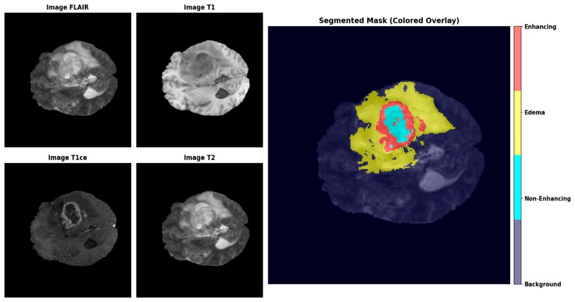
Figure 1. Magnetic Resonance Imaging (MRI) input modalities (FLAIR, T1, T1ce, and T2) with the corresponding segmented mask. Colour Key: yellow indicates oedema, red represents the enhancing tumour, and blue denotes the non-enhancing/necrotic core tumour.
Informatics 13 00118 g001
Figure 2. Sample slices of pre-processed multimodal MRI data with corresponding ground-truth grey-scale and coloured segmentation masks (enhancing tumour, oedema, and necrotic core). Colour Key: yellow indicates oedema, red represents the enhancing tumour, and blue denotes the non-enhancing/necrotic core tumour.
Informatics 13 00118 g002
Figure 3. Proposed 3D MRI brain tumour segmentation methodology. Colour Key: yellow indicates oedema, red represents the enhancing tumour, and blue denotes the non-enhancing/necrotic core tumour.
Informatics 13 00118 g003
Figure 4. Proposed 3D U-Net model for brain tumour segmentation.
Informatics 13 00118 g004
Figure 5. Visual representation of activation functions and their derivatives.
Informatics 13 00118 g005
Figure 6. Validation Dice score convergence across 100 training epochs. The learning curves for the twelve activation functions demonstrate rapid initial convergence within the first 20 epochs, followed by stabilisation. Swish and TanhExp exhibit marginally higher final mean Dice scores than the ReLU baseline. While all models converge to a high-performance plateau (mean Dice > 0.75), Swish maintains a smooth, stable trajectory throughout the latter half of the training process.
Informatics 13 00118 g006
Figure 7. Reliability by region: 95% Hausdorff Distance (lower is better).
Informatics 13 00118 g007
Figure 8. Reliability analysis of various activation functions using 95% Hausdorff Distance (HD95) for the necrotic-core. The boxplot compares boundary delineation accuracy across 12 activation functions, where a lower HD95 value indicates better performance. While median values remain consistently low (under 5 mm) across all models, the presence of significant outliers (ranging up to 35 mm) suggests varying degrees of boundary instability for certain cases within the necrotic-core segmentation.
Informatics 13 00118 g008
Figure 9. Radar chart comparing Dice Similarity Coefficients (DSCs) for four representative activation functions (ReLU, Swish, PReLU and TanhExp) across the five tumour sub-regions. Scores span from approximately 0.66 in the challenging necrotic core to 0.88 in the whole tumour. TanhExp (red) shows a marginal lead in the whole tumour, while ReLU (black dashed) remains highly competitive in the tumour core; overall, the differences between functions are small across all regions.
Informatics 13 00118 g009
Figure 10. Qualitative comparison of tumour segmentation results across activation functions for a representative MRI slice. The panels display the segmentation of necrotic (red), enhancing (yellow), and oedema (green) tissue types against the ground truth. While most functions accurately capture the primary tumour mass, variations in the necrotic-core (NCR) Dice score (ranging from 0.235 to 0.907) highlight differences in boundary precision, with Swish and Leaky ReLU achieving high local accuracy (0.907 and 0.905, respectively) for this specific patient sample. ★ denotes the best-performing activation function (Swish).
Informatics 13 00118 g010
Figure 11. Qualitative segmentation performance. Comparative overlay for Patient 057 (Slice 82). (A) T1ce MRI slice. (B) Ground-truth overlay (Red: necrotic core (NCR), Yellow: enhancing tumour (ET), Green: oedema (ED)). (C) ReLU Prediction: The model fails to capture the central necrotic core (Slice Dice: 0.368). (D) Swish Prediction: Successfully delineates the core boundary (Slice Dice: 0.871), demonstrating superior structural preservation.
Informatics 13 00118 g011
Figure 12. Statistical stability analysis of necrotic-core segmentation. (A) Box plot of Dice scores showing that Swish achieves a higher median accuracy with a tighter interquartile range than the baseline. (B) Box plot of 95% Hausdorff Distance (HD95) for the necrotic core, where Swish shows a contained distribution comparable to HardELiSH and PReLU.
Informatics 13 00118 g012
Figure 13. Architectural Efficiency Dashboard (single-GPU, NVIDIA A100-SXM4-40 GB): (A) Per-epoch training latency versus segmentation accuracy. (B) Peak GPU memory versus mean Dice. Swish provides an optimal trade-off, achieving competitive accuracy at near-baseline latency and memory, whereas Logish, Mish, Smish and TanhExp incur ~1.3–1.4× latency and ~2.5× memory for no accuracy gain.
Informatics 13 00118 g013
Table 2. Detailed layer-by-layer specification of the improved 3D residual U-Net.
Block LevelOperation/Layer TypeInput ChannelsOutput ChannelsKernel SizeStrideActivation
Input3D MRI Modalities
(T1, T1ce, T2, FLAIR)
44---
Encoder 1Residual Block
(Conv BN Act) × 2
432 3 × 3 × 3 1Variable
Max Pooling 3D3232 2 × 2 × 2 2-
Encoder 2Residual Block
(Conv BN Act) × 2
3264 3 × 3 × 3 1Variable
Max Pooling 3D6464 2 × 2 × 2 2-
Encoder 3Residual Block
(Conv BN Act) × 2
64128 3 × 3 × 3 1Variable
Max Pooling 3D128128 2 × 2 × 2 2-
Encoder 4Residual Block
(Conv BN Act) × 2
128256 3 × 3 × 3 1Variable
Max Pooling 3D256256 2 × 2 × 2 2-
BottleneckResidual Block
(Conv BN Act) × 2
256512 3 × 3 × 3 1Variable
Decoder 4Transposed Conv 3D
(Upsample)
512256 2 × 2 × 2 2-
Concatenation with
Encoder 4
512512---
Residual Block
(Conv BN Act) × 2
512256 3 × 3 × 3 1Variable
Decoder 3Transposed Conv 3D
(Upsample)
256128 2 × 2 × 2 2-
Concatenation with
Encoder 3
256256---
Residual Block
(Conv BN Act) × 2
256128 3 × 3 × 3 1Variable
Decoder 2Transposed Conv 3D
(Upsample)
12864 2 × 2 × 2 2-
Concatenation with
Encoder 2
128128---
Residual Block
(Conv BN Act) × 2
12864 3 × 3 × 3 1Variable
Decoder 1Transposed Conv 3D
(Upsample)
6432 2 × 2 × 2 2-
Concatenation with
Encoder 1
6464---
Residual Block
(Conv BN Act) × 2
6432 3 × 3 × 3 1Variable
OutputConvolution 3D (Logits)324 1 × 1 × 1 1Linear
Bold denotes the header row and the network’s structural stages. “Variable” refers to the specific activation function being evaluated in that experimental fold, e.g., ReLU or Swish.
Table 3. Characteristics and formulas of activation functions used in this study.
Activation FunctionMathematical FormulaCharacteristics
ReLU [23] f x = m a x 0   ,   x ,
where x is the input of the neuron
Computational efficiency; induces sparsity; prone to “dying ReLU” problem.
Leaky ReLU [24] f x = x ,     x 0 α x ,     x < 0
where α 0.01
Addresses the dying ReLU problem by permitting a small, non-zero gradient for negative input values.
PReLU [25] f x = x ,     x 0 α x ,     x < 0 Similar to Leaky ReLU, but α is a learnable parameter during training.
ELU [27] f x = x , x 0 α ( e x 1 ) , x < 0 Smoother than ReLU; pushes mean activations closer to zero; robust to noise.
GELU [28] f x = 0.5 × 1 + tanh 2 π   x + 0.044715 x 3   Probabilistic; weights inputs by their percentile; smoother curvature than ReLU.
Swish [22] f ( x ) = x   σ ( x ) = x 1 + e x   Non-monotonic; smooth; self-gated; often outperforms ReLU in deep networks.
Mish [29] f x = x   tanh ( ln ( 1 + e x ) )     Self-regularised; non-monotonic; smooth; preserves small negative information.
EliSH [26] f x = x   σ ( x ) , x 0 e x 1 σ ( x )   , x < 0 Combines the benefits of ELU and Swish; handles negative values smoothly.
HardEliSH [26]   f x = x max 0 , min 1 , x + 1 2 ,   i f   x 1 e x 1 max 0 , min 1 , x + 1 2   i f   x < 0 A computationally faster, piecewise-linear approximation of ELiSH.
TanhExp [30] f x = x . tanh ( e x ) Exhibits characteristics of hyperbolic tangent and exponential functions. It helps in improving gradient flow by avoiding issues of vanishing gradients in deep nets.
Logish [31] f ( x ) = x . ln ( 1 + 1 1 + e x ) Has a smooth sigmoid-like curve, which produces output in a given range, thus increasing the non-linearity of the model. It improves the gradient flow by preventing the output from saturating to extremes.
Smish [32]       f x = x . t a n h ( ln   1 + 1 1 + e x ) Has a smooth, non-linear form, which incorporates the properties of both the Swish and sigmoid functions, providing unbounded positive output.
Bold denotes the activation-function names (row labels).
Table 4. Summary of evaluation metrics and their formulas and characteristics.
MetricsMathematical FormulaCharacteristics
Accuracy T P   + T N   T P   + F P   + T N   + F N Overall pixel-wise correctness; can be misleading with class imbalance.
Precision T P   T P   + F P   Reliability of positive predictions; crucial when false positives are costly.
Recall (Sensitivity) T P   T P   + F N   Ability to detect all positive cases; crucial when false negatives are costly.
Dice Similarity Coefficient (F1-Score)     2 × P r e c i s i o n   ×   R e c a l l P r e c i s i o n + R e c a l l Robust overlap measure balancing precision/recall; widely used for imbalanced segmentation.
Specificity T N   T N   + F P   Correct identification of negative cases; important for confidently ruling out disease.
Jaccard Index T P   T P   + F p   + F N   Intersection over Union; robust measure of overall segmentation overlap and localisation.
Hausdorff Distance H A , B = max max a A min b B a b , max b B min a A b a Maximum boundary discrepancy; critical for assessing precise edge delineation.
Mean IoU I o U = I n t e r s e c t i o n U n i o n =   A p r e d A g t A p r e d A g t Average segmentation quality across all classes; balances class performance.
Table 5. Dice Similarity Coefficient (DSC) across tumour sub-regions.
ActivationETTCWTNCRED
Logish0.805 ± 0.089
[0.783, 0.824]
0.866 ± 0.110
[0.839, 0.889]
0.877 ± 0.091 *
[0.854, 0.896]
0.670 ± 0.236 **
[0.613, 0.721]
0.791 ± 0.131 *
[0.760, 0.819]
Smish0.801 ± 0.101
[0.777, 0.823]
0.860 ± 0.118
[0.832, 0.886]
0.871 ± 0.102
[0.846, 0.892]
0.661 ± 0.237
[0.606, 0.713]
0.785 ± 0.139
[0.751, 0.816]
TanhExp0.811 ± 0.077 *
[0.794, 0.828]
0.864 ± 0.118
[0.836, 0.888]
0.879 ± 0.084 **
[0.859, 0.897]
0.665 ± 0.244 *
[0.607, 0.717]
0.791 ± 0.127 **
[0.761, 0.819]
ReLU0.805 ± 0.083
[0.786, 0.824]
0.871 ± 0.097
[0.849, 0.891]
0.871 ± 0.090
[0.850, 0.891]
0.663 ± 0.230
[0.609, 0.714]
0.782 ± 0.137
[0.749, 0.812]
Leaky ReLU0.809 ± 0.085
[0.789, 0.827]
0.866 ± 0.104
[0.840, 0.888]
0.877 ± 0.084 **
[0.858, 0.896]
0.659 ± 0.255
[0.600, 0.716]
0.790 ± 0.134 **
[0.759, 0.819]
PReLU0.794 ± 0.116
[0.766, 0.818]
0.846 ± 0.145 **
[0.811, 0.877]
0.866 ± 0.110
[0.837, 0.888]
0.664 ± 0.248 *
[0.606, 0.719]
0.775 ± 0.149
[0.740, 0.807]
ELU0.808 ± 0.087 *
[0.787, 0.828]
0.867 ± 0.109
[0.841, 0.891]
0.874 ± 0.093
[0.851, 0.893]
0.671 ± 0.237 **
[0.615, 0.724]
0.786 ± 0.132
[0.754, 0.815]
GELU0.797 ± 0.096
[0.773, 0.817]
0.854 ± 0.117 **
[0.826, 0.879]
0.874 ± 0.085
[0.854, 0.892]
0.670 ± 0.241 *
[0.612, 0.723]
0.787 ± 0.132
[0.756, 0.815]
Swish0.812 ± 0.092 **
[0.790, 0.832]
0.864 ± 0.119
[0.835, 0.890]
0.871 ± 0.098
[0.847, 0.891]
0.676 ± 0.244 **
[0.618, 0.728]
0.784 ± 0.135
[0.753, 0.814]
Mish0.805 ± 0.109 **
[0.780, 0.829]
0.862 ± 0.127
[0.832, 0.890]
0.877 ± 0.083 **
[0.857, 0.895]
0.661 ± 0.258 *
[0.600, 0.718]
0.789 ± 0.128 *
[0.760, 0.817]
EliSH0.800 ± 0.132 *
[0.767, 0.827]
0.855 ± 0.156
[0.818, 0.888]
0.869 ± 0.115
[0.841, 0.893]
0.660 ± 0.260
[0.598, 0.719]
0.783 ± 0.142
[0.748, 0.814]
HardEliSH0.804 ± 0.081
[0.785, 0.822]
0.865 ± 0.102
[0.841, 0.886]
0.873 ± 0.080
[0.854, 0.890]
0.670 ± 0.235
[0.616, 0.722]
0.784 ± 0.129
[0.754, 0.813]
Best results are bold. Statistical significance vs. ReLU: * p < 0.05, ** p < 0.01. Values in square brackets are bootstrap 95% confidence intervals (5000 resamples). ET = Enhancing Tumour; TC = Tumour Core; WT = Whole Tumour; NCR = Necrotic Core; ED = Oedema.
Table 6. 95% Hausdorff Distance (lower is better) statistical significance vs. ReLU.
ActivationETTCWTNCR
EliSH2.269 ± 4.672 [1.43, 3.53]2.857 ± 5.601 [1.74, 4.25]2.338 ± 3.782 [1.62, 3.34]10.478 ± 43.489 [4.36, 21.47]
ELU2.011 ± 3.274 [1.41, 2.87]2.439 ± 4.244 [1.58, 3.52]2.392 ± 4.067 [1.60, 3.42]5.650 ± 6.592 [4.24, 7.25]
GELU1.941 ± 2.155 [1.51, 2.48]2.655 ± 4.540 [1.75, 3.83]2.627 ± 6.303 [1.54, 4.37]5.794 ± 6.475 [4.43, 7.33]
HardEliSH1.875 ± 2.634 [1.36, 2.55]2.529 ± 4.818 [1.59, 3.76]2.093 ± 2.493 [1.58, 2.70]5.691 ± 6.569 ** [4.31, 7.29]
Leaky ReLU1.794 ± 2.349 [1.33, 2.40]2.615 ± 4.108 [1.78, 3.63]2.843 ± 7.986 * [1.54, 5.00]6.450 ± 7.501 ** [4.89, 8.26]
Logish2.079 ± 2.814 [1.52, 2.79]2.331 ± 3.323 [1.63, 3.14]2.207 ± 3.376 [1.52, 3.04]5.604 ± 5.989 * [4.36, 7.11]
Mish2.256 ± 4.029 [1.48, 3.26]3.040 ± 5.293 [1.95, 4.34]2.259 ± 2.993 * [1.64, 2.97]5.940 ± 6.632 [4.57, 7.51]
PReLU2.532 ± 4.560 [1.62, 3.64]3.225 ± 5.329 ** [2.11, 4.57]2.618 ± 4.294 [1.76, 3.67]5.882 ± 6.922 [4.44, 7.52]
ReLU1.933 ± 2.522 [1.44, 2.57]2.278 ± 3.348 [1.60, 3.09]2.497 ± 3.568 [1.77, 3.39]5.315 ± 6.404 [3.96, 6.89]
Smish2.173 ± 3.547 [1.49, 3.10]2.508 ± 4.070 [1.69, 3.53]2.395 ± 3.526 [1.68, 3.30]5.549 ± 5.906 [4.30, 6.96]
Swish2.130 ± 3.496 [1.46, 3.02]2.858 ± 5.327 [1.76, 4.19]2.539 ± 3.757 [1.77, 3.45]6.039 ± 7.181 [4.52, 7.76]
TanhExp2.256 ± 3.791 [1.50, 3.26]2.948 ± 5.780 [1.80, 4.42]2.101 ± 2.828 * [1.53, 2.80]5.749 ± 6.668 [4.32, 7.39]
Best results are bold. Statistical significance vs. ReLU: * p < 0.05, ** p < 0.01. Values in square brackets are bootstrap 95% confidence intervals (5000 resamples).
Table 7. Sensitivity (recall)—ability to detect tumour tissue. Statistical significance vs. ReLU.
ActivationETTCWTNCRED
EliSH0.832 ± 0.158 ** [0.792, 0.865]0.848 ± 0.162 ** [0.807, 0.882]0.875 ± 0.148 [0.839, 0.906]0.632 ± 0.256 [0.571, 0.687]0.808 ± 0.167 * [0.768, 0.845]
ELU0.823 ± 0.131 ** [0.792, 0.852]0.849 ± 0.117 ** [0.821, 0.875]0.865 ± 0.134 ** [0.833, 0.893]0.647 ± 0.239 [0.588, 0.698]0.794 ± 0.165 [0.755, 0.831]
GELU0.790 ± 0.136 ** [0.758, 0.820]0.810 ± 0.134 ** [0.778, 0.840]0.876 ± 0.117 ** [0.847, 0.900]0.621 ± 0.245 ** [0.562, 0.676]0.821 ± 0.151 ** [0.785, 0.854]
HardEliSH0.824 ± 0.115 ** [0.796, 0.850]0.831 ± 0.119 ** [0.804, 0.858]0.895 ± 0.107 ** [0.869, 0.918]0.602 ± 0.244 ** [0.547, 0.657]0.841 ± 0.140 ** [0.808, 0.872]
Leaky ReLU0.840 ± 0.107 ** [0.816, 0.864]0.847 ± 0.106 ** [0.823, 0.871]0.887 ± 0.111 [0.859, 0.910]0.611 ± 0.231 ** [0.558, 0.663]0.827 ± 0.147 ** [0.793, 0.859]
Logish0.829 ± 0.126 ** [0.799, 0.858]0.849 ± 0.119 ** [0.821, 0.874]0.869 ± 0.127 ** [0.839, 0.897]0.633 ± 0.237 ** [0.578, 0.686]0.801 ± 0.159 * [0.762, 0.835]
Mish0.837 ± 0.141 ** [0.803, 0.867]0.863 ± 0.101 ** [0.840, 0.885]0.881 ± 0.114 [0.853, 0.904]0.645 ± 0.234 * [0.589, 0.698]0.810 ± 0.152 * [0.774, 0.844]
PReLU0.789 ± 0.151 ** [0.754, 0.822]0.822 ± 0.144 ** [0.787, 0.853]0.848 ± 0.145 ** [0.813, 0.879]0.651 ± 0.248 [0.592, 0.706]0.776 ± 0.178 ** [0.734, 0.817]
ReLU0.857 ± 0.107 [0.832, 0.880]0.882 ± 0.097 [0.859, 0.903]0.884 ± 0.121 [0.854, 0.909]0.651 ± 0.237 [0.595, 0.703]0.804 ± 0.160 [0.766, 0.840]
Smish0.817 ± 0.136 ** [0.784, 0.845]0.843 ± 0.137 ** [0.811, 0.872]0.861 ± 0.137 ** [0.829, 0.890]0.641 ± 0.241 [0.584, 0.694]0.792 ± 0.164 ** [0.752, 0.827]
Swish0.818 ± 0.134 ** [0.785, 0.846]0.840 ± 0.124 ** [0.811, 0.866]0.866 ± 0.139 ** [0.833, 0.895]0.645 ± 0.236 [0.588, 0.699]0.800 ± 0.170 [0.759, 0.837]
TanhExp0.848 ± 0.096 * [0.826, 0.869]0.859 ± 0.100 ** [0.836, 0.881]0.879 ± 0.117 ** [0.850, 0.904]0.633 ± 0.235 ** [0.578, 0.685]0.807 ± 0.152 [0.771, 0.840]
Best results are bold. Statistical significance vs. ReLU: * p < 0.05, ** p < 0.01. Values in square brackets are bootstrap 95% confidence intervals (5000 resamples).
Table 8. Precision (PPV)—ability to exclude false positives. Statistical significance vs. ReLU.
ActivationETTCWTNCRED
EliSH0.801 ± 0.107 ** [0.776, 0.825]0.893 ± 0.137 ** [0.859, 0.922]0.888 ± 0.086 ** [0.867, 0.907]0.775 ± 0.248 ** [0.716, 0.828]0.794 ± 0.142 [0.761, 0.825]
ELU0.814 ± 0.099 ** [0.790, 0.836]0.903 ± 0.122 ** [0.872, 0.928]0.903 ± 0.076 ** [0.884, 0.918]0.781 ± 0.223 ** [0.730, 0.829]0.809 ± 0.136 ** [0.778, 0.839]
GELU0.828 ± 0.102 ** [0.803, 0.850]0.923 ± 0.115 ** [0.895, 0.946]0.888 ± 0.087 ** [0.867, 0.906]0.803 ± 0.235 ** [0.745, 0.853]0.778 ± 0.149 * [0.741, 0.810]
HardEliSH0.804 ± 0.108 ** [0.779, 0.828]0.918 ± 0.115 ** [0.889, 0.942]0.867 ± 0.099 ** [0.843, 0.888]0.835 ± 0.205 ** [0.786, 0.879]0.760 ± 0.154 ** [0.724, 0.793]
Leaky ReLU0.797 ± 0.116 ** [0.770, 0.823]0.903 ± 0.136 ** [0.871, 0.932]0.882 ± 0.092 ** [0.861, 0.903]0.808 ± 0.266 ** [0.745, 0.866]0.778 ± 0.154 ** [0.741, 0.812]
Logish0.802 ± 0.108 ** [0.775, 0.826]0.903 ± 0.125 ** [0.872, 0.928]0.903 ± 0.081 ** [0.883, 0.920]0.798 ± 0.215 ** [0.745, 0.844]0.810 ± 0.135 ** [0.778, 0.839]
Mish0.803 ± 0.112 ** [0.777, 0.826]0.882 ± 0.160 ** [0.843, 0.915]0.887 ± 0.090 ** [0.866, 0.907]0.767 ± 0.272 ** [0.704, 0.827]0.795 ± 0.142 [0.762, 0.826]
PReLU0.828 ± 0.109 ** [0.802, 0.851]0.898 ± 0.160 ** [0.860, 0.931]0.906 ± 0.080 ** [0.887, 0.924]0.779 ± 0.227 ** [0.724, 0.827]0.807 ± 0.141 ** [0.774, 0.839]
ReLU0.777 ± 0.115 [0.751, 0.802]0.875 ± 0.122 [0.844, 0.900]0.877 ± 0.096 [0.855, 0.897]0.747 ± 0.224 [0.693, 0.796]0.788 ± 0.152 [0.752, 0.822]
Smish0.808 ± 0.108 ** [0.783, 0.833]0.897 ± 0.116 ** [0.869, 0.921]0.902 ± 0.084 ** [0.882, 0.920]0.763 ± 0.235 * [0.708, 0.815]0.810 ± 0.141 ** [0.776, 0.841]
Swish0.827 ± 0.096 ** [0.806, 0.848]0.906 ± 0.134 ** [0.873, 0.934]0.896 ± 0.080 ** [0.877, 0.914]0.784 ± 0.247 ** [0.725, 0.836]0.800 ± 0.132 [0.770, 0.831]
TanhExp0.794 ± 0.111 ** [0.767, 0.817]0.887 ± 0.147 ** [0.850, 0.917]0.894 ± 0.082 ** [0.874, 0.912]0.791 ± 0.239 ** [0.734, 0.842]0.800 ± 0.135 * [0.768, 0.830]
Best results are bold. Statistical significance vs. ReLU: * p < 0.05, ** p < 0.01. Values in square brackets are bootstrap 95% confidence intervals (5000 resamples).
Table 9. Computational cost comparison (ReLU vs. Swish).
MetricReLU
(Baseline)
Swish
(Proposed)
Overhead/
Difference
Trainable Parameters22.93 M22.93 M+0 (No change)
GFLOPs (Forward Pass)491.28491.28+0 (Negligible)
Peak VRAM (Train, Batch = 2)5.80 GB6.96 GB+ 1.16 GB
Training Time (per Epoch)25.34 s25.57 s+ 0.23 s (~1%)
Inference Time (per Volume)~28 ms~28 mscomparable
Note: Hardware profiling was conducted on a single NVIDIA A100-SXM4-40 GB GPU; peak VRAM is the maximum allocated memory during training. Full 12-function timings are in Supplementary Table S2. Inference time is activation-independent (~28 ms/volume); the higher ReLU figure in the raw timing log reflects a one-off validation-data caching cost. Bold indicates the best value in each column.
Table 10. Comparison of the proposed model against published U-Net and Transformer benchmarks on the BraTS dataset.
ArchitectureStudyBraTS EditionDice WTDice TCDice ET
3D Residual U-Net (baseline, ReLU)This study20200.8710.8710.805
3D Residual U-Net (proposed, Swish)This study20200.8710.8640.812
nnU-Net (challenge winner)Isensee et al. [47]20200.8900.8510.820
TransBTSWang et al. [52]2020 †0.9010.8170.787
Attention U-NetOktay et al. [60] ‡20190.8880.7720.760
Swin UNETRHatamizadeh et al. [51]20210.9260.8850.858
Best result among the proposed models is shown in bold. † TransBTS BraTS 2020 validation with test-time augmentation; ‡ Attention U-Net BraTS 2019 results as reported by Wang et al. [52]. UNETR [53] is not tabulated because its published brain tumour evaluation uses the Medical Segmentation Decathlon task rather than BraTS. State-of-the-art methods typically rely on ensembling, test-time augmentation and/or larger BraTS editions, whereas the present study reports a single lightweight model.
Table 11. Across-seed Dice (mean ± SD over seeds 42/1337/2025).
ActivationETTCWTNCRED
ReLU0.808 ± 0.0040.865 ± 0.0070.875 ± 0.0020.661 ± 0.0120.787 ± 0.005
Swish0.801 ± 0.0110.861 ± 0.0080.875 ± 0.0050.677 ± 0.0030.789 ± 0.006
PReLU0.800 ± 0.0070.862 ± 0.0070.875 ± 0.0030.678 ± 0.0040.789 ± 0.003
TanhExp0.810 ± 0.0040.865 ± 0.0040.876 ± 0.0060.666 ± 0.0040.787 ± 0.007
Table 12. Five-fold cross-validation—across-fold Dice (mean ± SD over folds, out-of-fold predictions).
ActivationETTCWTNCRED
ReLU0.754 ± 0.0370.827 ± 0.0270.903 ± 0.0150.655 ± 0.0340.778 ± 0.026
Swish0.755 ± 0.0360.832 ± 0.0280.903 ± 0.0150.663 ± 0.0350.778 ± 0.022
PReLU0.760 ± 0.0310.826 ± 0.0220.902 ± 0.0140.652 ± 0.0310.778 ± 0.025
TanhExp0.757 ± 0.0360.831 ± 0.0220.902 ± 0.0180.660 ± 0.0270.780 ± 0.024
Disclaimer/Publisher’s Note: The statements, opinions and data contained in all publications are solely those of the individual author(s) and contributor(s) and not of MDPI and/or the editor(s). MDPI and/or the editor(s) disclaim responsibility for any injury to people or property resulting from any ideas, methods, instructions or products referred to in the content.