
Article

Mapping Sub-Field Crop Water Use Dynamics Using OpenET Data and Zero-Shot Time-Series Foundation Model

by
Chinmay Deval
1,2 and
Siddharth Chaudhary
1,2,*
1
Earth System Science Center, The University of Alabama in Huntsville, 320 Sparkman Drive, Huntsville, AL 35899, USA
2
NASA Marshall Space Flight Center, Huntsville, AL 35808, USA
*
Author to whom correspondence should be addressed.
Informatics 2026, 13(6), 95; https://doi.org/10.3390/informatics13060095
Submission received: 5 May 2026 / Revised: 10 June 2026 / Accepted: 15 June 2026 / Published: 18 June 2026

Abstract

Precision agriculture increasingly relies on high-resolution, long-term remote sensing to delineate sub-field management zones. However, traditional spatial zonation assumes temporal stationarity, utilizing seasonal aggregates that obscure transient, intra-annual stress signals. This study develops a data-driven framework to characterize both persistent and non-stationary crop water use dynamics by integrating monthly, 30-m evapotranspiration (ET) data from OpenET (2000–2025) with zero-shot temporal anomaly detection. A pre-trained time-series foundation model (Chronos-T5-Small) generated counterfactual expectations for sub-field ET, quantifying deviations using a mean absolute error-based anomaly score. Unsupervised clustering of these anomaly scores with longitudinal ET metrics partitioned the landscape into dynamic biophysical regimes. Cross-registered against legacy persistence mapping based on seasonal totals, the foundation model showed strong directional agreement (86.1%, Cohen’s Kappa = 0.716) in identifying chronically constrained zones across 869 shared active pixels. Crucially, the framework identified 966 historically persistent pixels undergoing stability decay, of which 95.3% were statistically verified via paired t-tests to have collapsed into the field’s baseline variance pool. Furthermore, counterfactual anomaly detection isolated zones of recent acute divergence, differentiating enduring edaphic constraints from sudden system disruptions. This approach demonstrates how foundation models can transition from purely predictive engines to diagnostic instruments, advancing operational precision agriculture.

1. Introduction

The increasing demand for sustainable agricultural production under climate variability has intensified the need for high-resolution, data-driven monitoring of agroecosystem dynamics. Precision agriculture operates on the foundational premise that agricultural fields are inherently heterogeneous; sub-field variability in soil properties, topography, and historical management drives profound spatial differences in crop performance [1]. Historically, the delineation of sub-field management zones relied heavily on yield monitor data or intensive, in situ soil sampling. However, the advent of high-resolution remote sensing has transformed this paradigm, enabling spatially explicit observation of crop vigor, water use, and environmental conditions across continuous spatial and temporal scales [2]. In this context, precision agriculture integrates geospatial data, remote sensing technologies, and analytical frameworks to optimize input allocation, improve production and water use efficiency, reduce environmental impacts, and inform agronomic decision-making [3].
Among remotely sensed variables, evapotranspiration (ET) provides a physically grounded and integrative measure of crop water use that links plant physiological processes with land–atmosphere energy exchanges [4,5]. Satellite-based ET products have been widely applied to characterize within-field variability, assess irrigation demand, and identify zones of chronic water stress [6,7]. The emergence of OpenET, a multi-model ensemble platform providing 30 m monthly ET estimates across the Contiguous United States, has substantially expanded the temporal depth and spatial resolution of publicly available ET data [8,9]. This has created new opportunities for long-term analysis of sub-field crop water use dynamics as well as identification of persistent and emerging patterns in sub-field consumptive water use. In irrigated systems, long-term ET analyses have demonstrated that temporally stable patterns of crop water use can reliably inform precision management strategies. Prior work in Idaho’s Magic Valley has demonstrated that temporally stable patterns of sub-field crop water use, derived from multi-year seasonal totals, can serve as robust indicators of sub-field management zones [10,11]. Persistent high- and low-performing zones linked to soil physical properties, topographic variation, and other drivers were identified by normalizing ET to the field average and applying pixel-level hypothesis testing over a 16-year seasonal total record, providing an operational baseline for variable rate management (VRM) guidance [10]. These approaches have proven highly effective for isolating persistently high and low crop water use zones based on seasonal ET totals, aligning with established temporal stability theories in ecohydrology [6,12].
However, the reliance on long-term seasonal aggregation such as those used in these previous studies [10] carries a critical, often unexamined limitation of assuming temporal stationarity. Approaches based on seasonal totals assume that the spatial structure of crop water use, driven by static edaphic properties, remains largely consistent over time. In practice, modern agricultural systems are highly dynamic. Intra-annual changes in mechanical infrastructure (e.g., center-pivot nozzle degradation), biological stressors (e.g., localized pest outbreaks), or acute environmental conditions can rapidly alter system behavior. These non-stationary disruptions cause historically persistent zones to degrade, shift, or completely collapse. Because seasonal aggregation inherently smooths over sub-seasonal variance, traditional methods fundamentally obscure these transient disturbances and emerging stress signals until they manifest as permanent yield losses. This limitation highlights a critical unmet need: the ability to detect acute deviations from expected system behavior as they occur, enabling early identification of operational failures that persistence-based approaches are fundamentally unable to capture.
Concurrently, machine learning has transformed agricultural analytics, offering new pathways to model complex temporal dynamics [13]. Yet, the application of deep learning in agricultural remote sensing has traditionally relied on supervised learning paradigms that require extensive labeled datasets, which severely limits their scalability across diverse agroecological regions [14]. Furthermore, traditional time-series forecasting models struggle to capture the highly nonlinear, compound dynamics of climate-crop interactions without continuous, localized fine-tuning. More recently, a new class of artificial intelligence tools, like the time-series foundation models such as Google’s TimeFM [15] and Amazon’s Chronos [16], have emerged with the capacity to learn generalizable temporal dynamics from large, diverse training corpora and apply zero-shot forecasting to novel time series without domain-specific fine-tuning. These models offer a fundamentally different lens for analyzing ET time series: rather than summarizing historical behavior, they can generate an expectation of what a pixel’s behavior should look like given its history, against which the actual observed behavior can be compared. When cast as a counterfactual baseline, the model’s output does not simply forecast the crop water use. Rather, it diagnoses the present, revealing whether a pixel is behaving consistently with its historical state or has undergone a structural shift.
This reframing is the central conceptual contribution of this study. We apply Chronos-T5-Small [16], a pre-trained zero-shot time-series foundation model, in a counterfactual anomaly detection mode to 25 years of monthly OpenET data across four irrigated center-pivot fields in the Magic Valley, Idaho. Model-generated counterfactual expectations are compared against observed ET to generate pixel-level anomaly scores. These are combined with three longitudinal relative ET indicators, which capture long-term transpiration capacity, system stability, and temporal persistence within an unsupervised K-Means clustering framework. This produces five distinct biophysical regimes that represent both stable edaphic structure and dynamic system transitions.
The key research question this study addresses is: Can long-term, monthly satellite-derived ET data be leveraged without labeled training data to simultaneously map stable sub-field management zones and detect their breakdown through non-stationary analysis? We validate our framework against the legacy persistence baseline maps [10] and confirm detected stability decay using paired t-tests on raw seasonal total ET. This integrated approach advances the use of satellite remote sensing and foundation models in precision agriculture from static spatial classification to dynamic inference of system-state evolution, providing operational guidance that is both spatially explicit and temporally responsive.

2. Materials and Methods

2.1. Study Area and Agronomic Context

This study was conducted at four center-pivot fields within the Idaho Center for Agriculture, Food, and the Environment (Idaho CAFE) Sustainable Water and Soil Health Demonstration Farm near Rupert, Idaho, USA [10,17]. The fields were established in March 2019 and have been used for evaluating sustainable water and soil management practices. Before the establishment of the demonstration farm, the fields were managed under a conventional four-year crop rotation that included sugar beet (Beta vulgaris), barley (Hordeum vulgare), and potato (Solanum tuberosum), with regular applications of inorganic fertilizers [17]. These fields are located in the Magic Valley region of southern Idaho, which has a semi-arid climate characterized by hot summers and cold winters. Average annual precipitation is approximately 280 mm, with most precipitation occurring as snowfall during winter [18]. Consequently, agricultural production in the region relies on irrigation from the Snake River and groundwater resources [18,19]. Mean annual temperature is 7.8 °C, with temperatures typically ranging from 0 to 15.6 °C [17]. The soils are primarily derived from volcanic materials, including basalt, and are generally well drained and fertile [20].

2.2. Data Acquisition and Preprocessing

A 25-year (2000–2025) monthly time series of pixel-level evapotranspiration (ET) estimates was extracted at 30 m spatial resolution using the OpenET ensemble product for the growing season months of April through October, yielding seven monthly observations per year and 175 total time steps across the study period. In contrast to the previous study [10], monthly rather than seasonal total ET values were used to preserve within-season temporal structure and enable the autoregressive pattern learning required by the foundation model. To isolate localized edaphic and management constraints from macroscopic inter-annual climate variability, raw ET values were normalized to a dimensionless Relative ET (relET) metric. For a given pixel i at time step t (representing a specific month and year), relET is calculated as the quotient of the pixel’s actual ET and the spatial mean of the entire field (N pixels) for that identical time step:
r e l E T p , t = E T p , t 1 n i = 1 n E T i , t
This normalization ensures a spatial mean of approximately 1.0 at every time step, effectively detrending the longitudinal dataset from seasonal phenology and regional meteorological anomalies, thereby isolating the site-specific spatial heterogeneity.

2.3. Historical Baseline Profiling

To characterize the fundamental physical properties of the landscape, the 25-year relET sequence for each pixel was collapsed into three longitudinal summary statistics. These metrics represent the long-term hydrologic behavior of the soil–canopy system:
Long-Term Transpiration Capacity (μET): Calculated as the temporal arithmetic mean of all observations. This metric serves as a normalized baseline of the localized ecohydrological performance, representing the fundamental ability of the soil–canopy system to sustain water flux independent of macroscopic climate trends.
μ r e l E T = 1 N t = 1 N r e l E T t
System Stability (σET): Calculated as the temporal standard deviation, quantifying the pixel’s sensitivity to environmental variance.
σ r e l E T = 1 N 1 t = 1 N ( r e l E T t μ r e l E T ) 2
Temporal Persistence (Ptemp): Calculated via Lag-1 Autocorrelation to measure the autoregressive memory of the soil (e.g., deep clay vs. highly drained sand).
P t e m p = t = 1 N 1 ( r e l E T t   μ r e l E T ) ( r e l E T t + 1   μ r e l E T ) t = 1 N ( r e l E T t   μ r e l E T ) 2

2.4. Zero-Shot Temporal Anomaly Detection

While longitudinal statistics effectively characterize chronic edaphic constraints, they cannot identify recent, non-stationary system shifts, which represents the central limitation of persistence-only frameworks. To address this, we applied Chronos-T5-Small [16], a pre-trained autoregressive time-series foundation model trained on a large and diverse corpus of real and synthetic time series, to perform zero-shot probabilistic forecasting on each pixel’s monthly relET sequence without any domain-specific training or fine-tuning. The selection of the Chronos-T5-Small variant was a deliberate design choice aimed at balancing zero-shot predictive performance with the computational constraints of large-scale, pixel-level agrohydrological monitoring. As demonstrated in recent benchmarking studies [21], while larger foundation models (e.g., Time-MoE or Moirai-2) provide significant predictive gains in specific economic forecasting contexts, they incur substantial memory and latency overheads. Furthermore, research has demonstrated that foundation models consistently outperform traditional statistical and bespoke deep learning methods in zero-shot settings [22]. By opting for the Chronos-T5-Small architecture, we leverage the robust, pre-trained temporal representations of foundation models while maintaining an inference speed and memory footprint suitable for high-throughput spatio-temporal data, ensuring both scalability and scientific reproducibility.
For each pixel, the temporal sequence was partitioned into a historical context window (the initial baseline years, spanning 2000–2024) and an 8-step hold-out window representing the 2025 growing season, the most recent complete annual observation period. The historical context tensor was passed to the Chronos pipeline, which generated a probabilistic forecast for the hold-out window, sampling 100 trajectories to characterize predictive uncertainty. A Chronos Anomaly Score (Ascore) was derived using the Mean Absolute Error (MAE) between the median model expectation ( r e l E T p r e d , m ) and the actual observed values (   r e l E T o b s , m ) over the final M months:
A s c o r e = 1 M m = 1 M |   r e l E T o b s , m   r e l E T p r e d , m
where M = 8. A high anomaly score indicates that a pixel’s behavior during the 2025 growing season deviated substantially from what the model expected based on its 24-year history. By treating the model output as a counterfactual baseline, defined as the expected behaviour given the historical relative dynamics, rather than a conventional forecast, deviations are interpretable as diagnostic signals of system state change rather than simple prediction error. The 80th percentile prediction interval (10th to 90th percentile of sampled trajectories) was also used to classify pixels whose observed values fell entirely outside the expected envelope as undergoing significant divergence. Inference was conducted in batches of 64 pixels on CPU using PyTorch (2.11.0) with float32 precision.

2.5. Unsupervised Spatial Zonation

To partition the continuous multidimensional feature space into discrete, actionable agronomic management zones, we applied an unsupervised K-Means clustering algorithm. Prior to clustering, the four engineered features were standardized to a mean of 0 and a variance of 1 to ensure equal weighting. Each pixel was represented as a 4-dimensional vector: xp = [μrelET, σrelET, Ascore, Ptemp].
The algorithm minimized the Within-Cluster Sum of Squares (WCSS) to partition the pixels into clusters. Cluster assignment was determined by minimizing the Euclidean distance between the pixel vector and the respective cluster centroids ck:
d ( xp , ck )   =   ( μ r e l E T μ k ) 2 + ( σ r e l E T σ k ) 2 + ( A s c o r e A k ) 2 + ( P t e m p P k ) 2
The k = 5 clusters naturally resolved into the following biophysical regimes:
  • Consistently Above Average: High μ r e l E T , high persistence, and low variance.
  • Baseline: μ r e l E T ≈ 1.0, moderate variance, representing the true field average.
  • Consistently Below Average: Low μ r e l E T and low variance, indicating permanent, moderate constraints.
  • Chronically Underperforming: Lowest μ r e l E T and highest historical variance.
  • Recent Acute Divergence: High historical μ r e l E T coupled with a maximum Ascore, identifying historically stable zones currently undergoing stability decay.

2.6. Statistical Corroboration of Algorithm Downgrades

To evaluate the validity and translational utility of the K-Means zonation, we compared the framework’s output against the 16-year legacy persistence baseline established for the same CAFE fields in the previous study [10]. The legacy method derived pixel-level persistence classifications using seasonal total ET from the University of Idaho/Idaho Department of Water Resources METRIC-based ET product (1986–2020), normalized to field-average relative crop water use (RCWU). Pixels whose time-series mean RCWU was statistically different from the field average at α = 0.05 were classified as persistently high or persistently low relative crop water use zones; all others were assigned to the baseline class. Critically, this legacy method uses seasonal aggregate totals and only one of the models used in OpenET, whereas the current framework operates on monthly time steps and uses an ensemble ET value, a fundamental methodological difference that enables detection of within-season dynamics not captured by annual summaries.
Validation was structured in two phases. First, directional agreement was quantified on the set of pixels where both methodologies detected a persistent spatial anomaly (i.e., both classified a pixel as non-baseline). For these 869 shared pixels, we computed a confusion matrix, overall directional accuracy, and Cohen’s Kappa coefficient to assess cross-methodological agreement in classifying the direction of the anomaly (high vs. low).
Second, pixels that the K-Means framework classified as Baseline (i.e., ‘downgraded’ from a legacy extreme), as well as pixels where both methods agreed, were subjected to a paired t-test (α = 0.05) comparing their raw seasonal total ET against the true field-average seasonal total ET for each year of the record. This provided a physically grounded verification: pixels that the model downgraded to baseline should show no statistically significant departure from the field mean, while pixels validated as persistent extremes should retain measurable physical separation. A pixel was classified as an ‘AI Downgrade (Proven True Baseline)’ if its t-test yielded p > 0.05, confirming that it no longer behaves as a physical extreme regardless of its historical classification.

3. Results

3.1. Biophysical Zonation of Sub-Field Crop Water Use

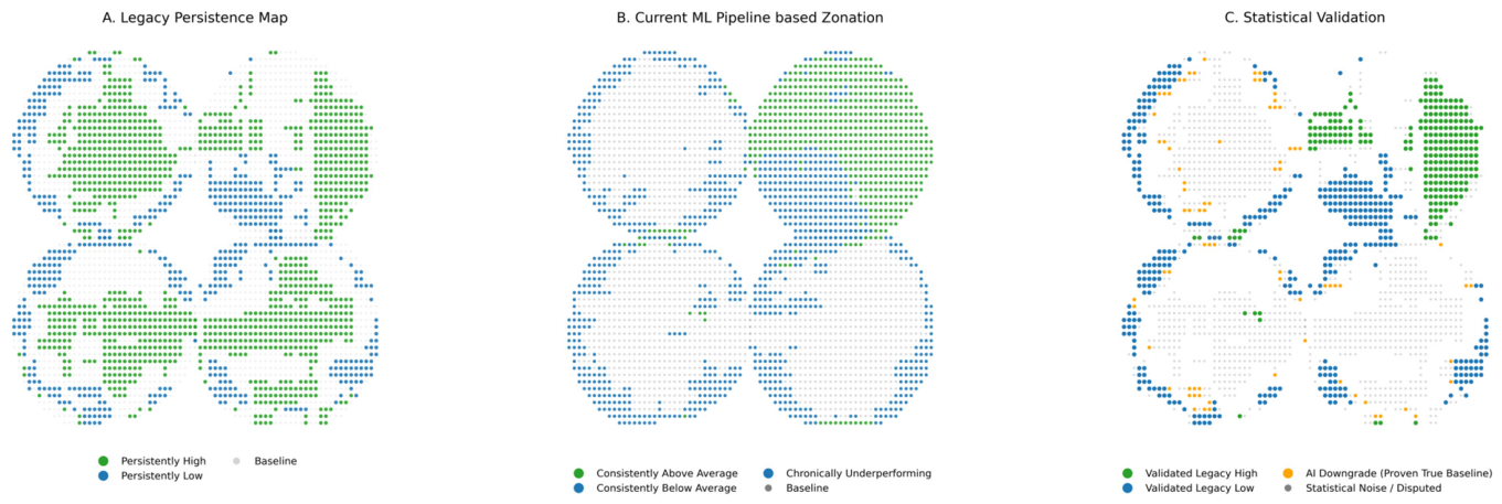
The unsupervised K-Means algorithm, applied to the four-dimensional feature space across four CAFE center-pivot fields, produced five spatially coherent and physically interpretable biophysical regimes (Figure 1A). The spatial arrangement of clusters reflects well-established patterns in irrigated center-pivot systems: Consistently Above Average pixels (green) concentrate toward the pivot center and in areas previously identified as high-performing by soil surveys, while Chronically Underperforming pixels (red) cluster at field peripheries, consistent with edge-effect dynamics documented in the previous study [10,11] and associated with shallow bedrock and advective stress. Baseline pixels (gray) form the spatial majority in each field, consistent with their mathematical definition as the modal class. Figure 1B overlays the Recent Acute Divergence pixels (purple) onto the historical zone map, revealing a spatial distribution of these divergences.

3.2. Spatial Concordance and the Identification of Stability Decay

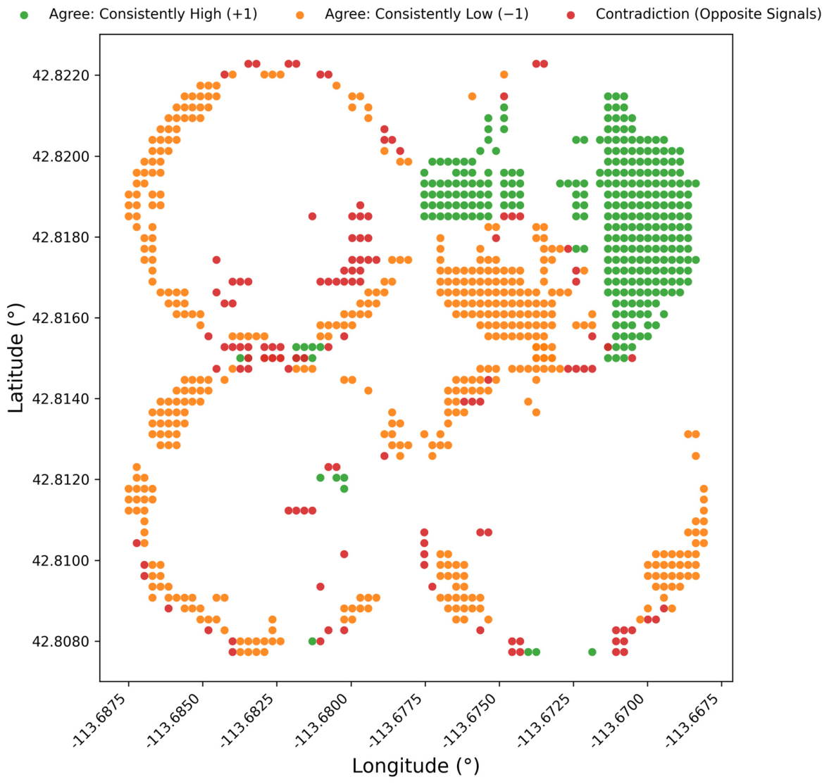
To evaluate whether the new monthly, AI-augmented framework reproduces the spatial information encoded in the established 16-year persistence baseline [10], we spatially co-registered the K-Means classifications against the legacy persistence map for the 869 pixels where both methodologies detected a persistent spatial anomaly (Figure 2 and Figure 3).
The confusion matrix for shared signals (Table 1) showed that 444 pixels were classified as Consistently Low by both methods, and 304 pixels were classified as Consistently High by both, for a total of 748 agreements. The remaining 121 pixels represented directional contradictions. This yields an overall directional accuracy of 86.1% and a Cohen’s Kappa coefficient of 0.716, indicating substantial cross-methodological agreement (Table 2). The Kappa value is particularly notable given that the two methods differ fundamentally in their temporal input (monthly vs. seasonal), mathematical approach (ML clustering vs. hypothesis testing), and temporal extent (25 vs. 16 years).
Agreement was heterogeneous across fields. Field 42 achieved the highest accuracy (97.3%, κ = 0.936), reflecting a field with strong, stable edaphic signals. Field 39 showed the lowest agreement (69.0%, κ = 0.038), suggesting more complex temporal dynamics or management-induced variability that the two methods resolve differently. The underlying causes for the near-zero κ at Field 39, potentially including depth to bedrock and within-field topographic differences [10], warrant further investigation. The cross-field variability in agreement reinforces that sub-field dynamics are field-specific and that no single aggregation method will uniformly capture all system states.

3.3. Statistical Corroboration of AI-Detected Non-Stationarity

A critical distinguishing feature of the K-Means framework is its classification of 966 pixels, previously designated as persistent extremes in the legacy baseline, into the Baseline cluster. Rather than treating this as classification error, we tested whether this ‘downgrade’ reflects genuine physical non-stationarity using seasonal total ET as an independent validation variable. For each downgraded pixel, we conducted a paired t-test (α = 0.05) comparing its seasonal total ET across all available years against the true field-average seasonal total ET computed from all pixels within the field for the same years.
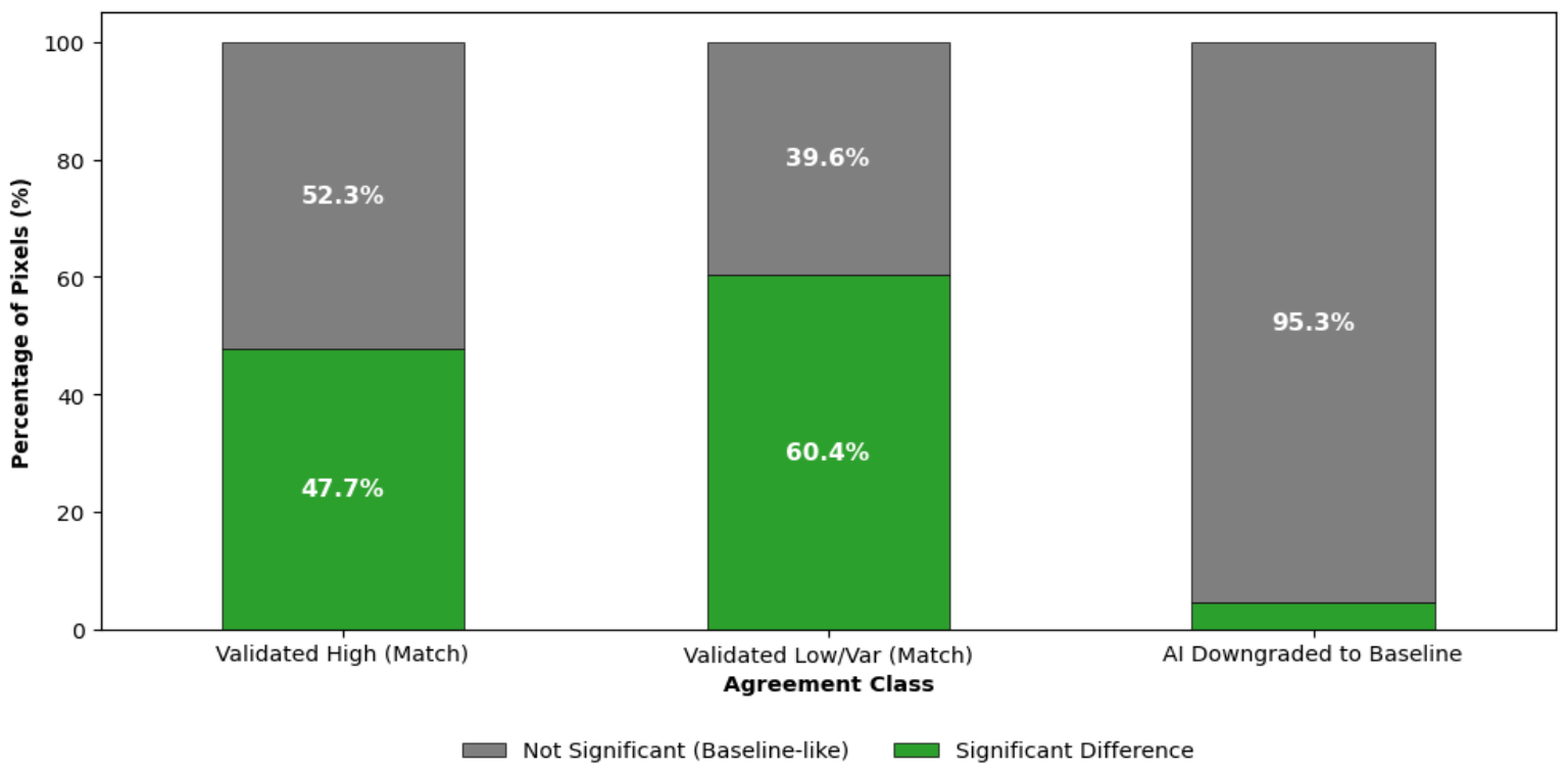
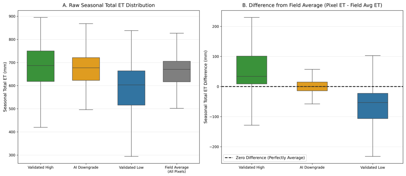
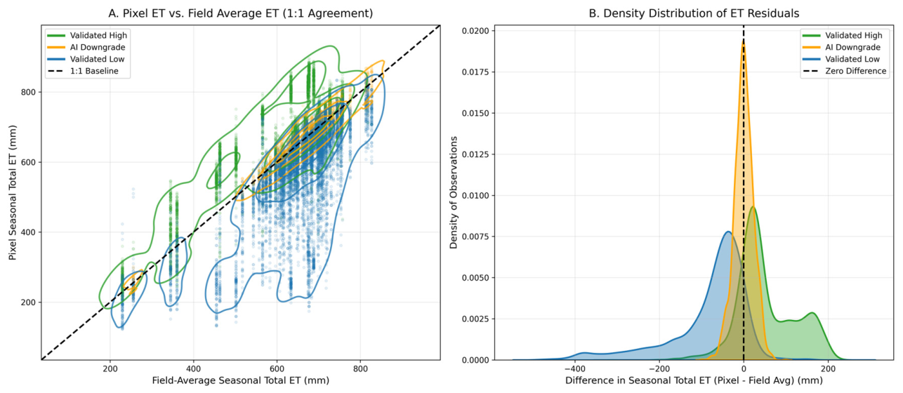
The results provided a strong statistical corroboration of the AI-driven reclassification (Figure 4, Figure 5 and Figure 6). Of the 966 downgraded pixels, 95.3% exhibited no statistically significant departure from the field-average seasonal total ET (p > 0.05), indicating an absence of consistent multi-year deviation from baseline conditions. This suggests that these pixels no longer exhibit persistent extreme behavior, but instead fluctuate within the natural variability of the field. Importantly, this does not imply strict equivalence to the field mean, but rather a loss of stable, repeatable divergence consistent with a transition from structured anomaly to background variability. In this context, the observed downgrades reflect stability decay: historical persistence patterns that have demonstrably collapsed back into the field’s natural variance pool.
In contrast, the framework correctly preserved the physical identity of validated extreme zones. For pixels classified as Validated Low/Var, where both methods agreed on a low-performing classification, 60.4% retained statistically significant departure from the field average (p < 0.05), confirming that genuine edaphic constraints were not false-positively erased by the new framework. For validated high pixels, 47.7% achieved strict statistical significance, while their interquartile ET range remained visibly elevated above the field baseline (Figure 5A), consistent with the inherently higher within-year variance characteristic of maximizing transpiration systems. Pixels assigned to the contradiction class, where the two methods assigned opposite directions, showed intermediate statistical separation (32.2% significant), consistent with their interpretation as spatially or temporally unstable zones lacking consistent directional behavior.

3.4. Detection of Transient Stress and Acute Anomalies

While the longitudinal statistical metrics captured chronic ecohydrological behavior, the zero-shot counterfactual baseline enabled the identification of an additional, qualitatively distinct class of behavior: transient, acute system disruption. The counterfactual framework established an expected relET trajectory for the final 8 months of the observation period (the 2025 growing season) by conditioning the Chronos-T5-Small model on each pixel’s historical context. A pixel was classified as exhibiting Recent Acute Divergence if its observed relET values during the hold-out window fell entirely outside the model’s 80% prediction interval (the 10th–90th percentile envelope of 100 sampled trajectories).
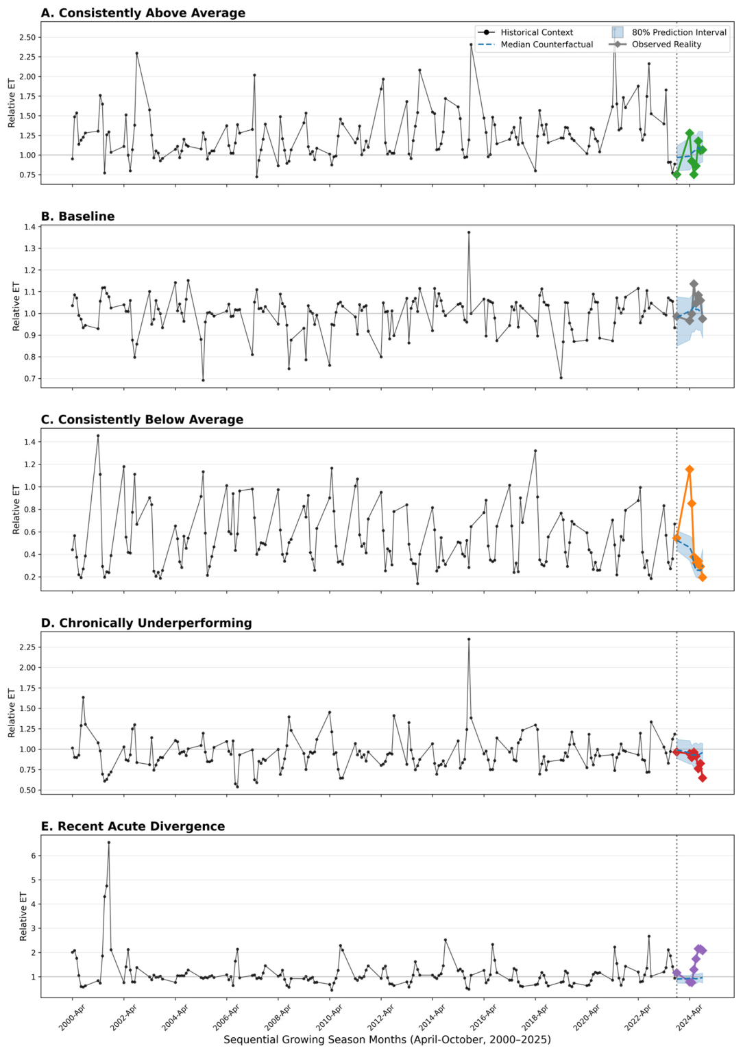
Figure 7 illustrates representative pixel time series for all five K-Means regimes, with the counterfactual expectation (dashed blue line) and 80% prediction interval (shaded ribbon) shown for the hold-out window. Panels A through D demonstrate that the model correctly anticipates the behavior of pixels in stable regimes: Consistently Above Average pixels receive a high counterfactual expectation and closely track it; Baseline pixels receive a near-unity expectation and are observed; accordingly, Consistently Below Average pixels receive a low expectation that reflects their persistent constraint. The Recent Acute Divergence panel (E) provides a stark contrast: for these pixels, which had stable, near-average histories, the model generates a reasonable expectation near relET = 1.0, but the observed 2025 values diverge sharply upward or downward, falling entirely outside the counterfactual envelope.
By framing the foundation model’s output as a counterfactual rather than a standard forecast, the pipeline effectively decouples a pixel’s current acute stress state from its historical baseline. This provides a critical operational distinction for precision agriculture: differentiating between areas that are chronically constrained by soil properties (requiring long-term amendment) and areas experiencing sudden mechanical or biological failures that diverge from their expected physical capability (requiring immediate intervention).

4. Discussion

The results demonstrate that integrating long-term monthly ET dynamics with a zero-shot time-series foundation model provides a fundamentally enhanced framework for characterizing sub-field agroecosystem heterogeneity, one that simultaneously preserves spatially coherent edaphic structure and detects its temporal breakdown. This dual capability addresses a core limitation of conventional persistence-based approaches, which by averaging across years implicitly assume that the spatial organization of crop water use is stationary.
The strong cross-methodological agreement observed between the framework presented in this study and the legacy baseline established in the previous study [10] provides important methodological validation. Despite operating on fundamentally different temporal inputs (monthly vs. seasonal totals), different mathematical frameworks (unsupervised ML clustering vs. pixel-level hypothesis testing), and different temporal extents (25 vs. 16 years, including some mismatching years), the two approaches converge strongly on the directional classification of persistent spatial anomalies. This convergence demonstrates that the monthly, AI-augmented framework maintains the core spatial structure of underlying soil and topographic constraints that the legacy method identified through independent physical analysis.
Agreement was asymmetric across the two directions of persistence, however. The framework exhibited substantially stronger recall for legacy low-performing zones (444 shared vs. 95 false-highs) than for high-performing zones (304 shared vs. 26 false-lows). This asymmetry is physically interpretable: areas of chronically low ET are often driven by hard physical limits such as shallow bedrock, coarse-textured soils with low water holding capacity that leave strong and stable imprints in the monthly time series regardless of management context. In contrast, high-performing zones often reflect more nuanced combinations of favorable soil depth, water access, and management optimization that may vary across the 25-year record as crop types, irrigation prescriptions, or equipment change. This interpretation aligns with the previous studies [10,11] on the same sites, which similarly observed that areas of persistently elevated water use were more sensitive to crop rotation and management-induced dynamics.
The most significant contribution of this work is the explicit identification and physical validation of stability decay, the collapse of historically persistent spatial patterns into statistically indistinguishable baseline behavior. Of the 966 pixels that the framework downgraded from legacy extreme to Baseline, 95.3% were confirmed by paired t-test to exhibit no statistically significant departure from the field-average seasonal total ET. This near-total correspondence between algorithmic downgrade and physical collapse provides strong evidence that the K-Means framework is not simply reclassifying stable patterns erroneously, but instead detects genuine system-state transitions that the legacy 16-year study could not reveal because it was computed over a period when those patterns were still active.
The implications are practically significant. Precision management strategies based on legacy persistence maps may lead to systematic misallocation of resources in areas where those patterns may no longer hold. This finding suggests that persistence maps derived from multi-decadal aggregates should be treated as temporally bounded products, requiring periodic revision as management practices, irrigation infrastructure, and soil conditions evolve. A framework capable of detecting this decay in near-real time, as presented here, provides the operational update mechanism that static persistence maps lack.
Monthly lagged ET information adds a key operational advantage by preserving within-season variability that is lost in seasonal aggregates. While seasonal totals support retrospective assessment, monthly trajectories retain the temporal structure needed to detect emerging deviations in crop water use during the growing season. In heterogeneous agroecosystems, these sub-seasonal signals enable earlier identification of shifts in field conditions, including both gradual stability decay and abrupt anomalies, thereby improving the timeliness of irrigation diagnostics and management response.
The detection of Recent Acute Divergence introduces a second, equally important capability: the identification of localized anomalies and sudden operational failures that are not easily explained by persistent environmental constraints. Some of these cluster along linear arcs within center-pivot fields, a pattern that can be consistent with irrigation system irregularities such as nozzle blockages or pressure variation. However, in this case, many of the affected pixels are located near field edges and have historically shown lower performance, raising the possibility of boundary or management effects.
Even so, the counterfactual approach remains useful: because the model defines an expected trajectory based on each pixel’s history, a sharp deviation from that expectation signals a departure from typical behavior, regardless of absolute productivity. These deviations may reflect short-term disturbances or operational issues but should be interpreted cautiously in edge areas.
This operational distinction between chronic constraints and acute anomalies enables fundamentally different management responses. Persistently underperforming zones driven by shallow bedrock or coarse soils require long-term structural interventions such as soil amendment, reclassification of management prescriptions, or targeted capital investment. Zones exhibiting Recent Acute Divergence, by contrast, require immediate field inspection and equipment diagnostics. Conflating these two signal types under a single framework would undermine actionable precision management.
The counterfactual formulation using model output not as a prediction of the future but as a diagnostic standard for the present represents a conceptual shift in how foundation models can be applied in environmental analysis. Rather than asking ‘what will happen next,’ the framework asks, ‘is this system behaving as it should, given its history?’ This framing is particularly suited to satellite-derived ET monitoring in agricultural fields, where the goal is not trajectory prediction but continuous system health assessment at the pixel scale for targeted management.
Several limitations of this study should be acknowledged. The k = 5 cluster solution was selected based on a combination of WCSS elbow analysis and domain-based interpretability constraints; alternative cluster solutions may reveal additional sub-regimes or merge classes that this analysis treats separately. The absence of concurrent yield maps, in situ soil moisture measurements, or irrigation system maintenance logs limits our ability to independently confirm the physical causes of detected anomalies, particularly for the Recent Acute Divergence class, which remains a spatially informed hypothesis rather than a confirmed diagnosis. The foundation model’s internal decision-making is not fully interpretable under current explainability tools, which may limit regulatory or operational trust in high-stakes precision management applications.
Future work should focus on expanding the validation to diverse crops, irrigation technologies, and ecohydrological settings to assess generalizability. Integration with soil physical property datasets, irrigation system telemetry, and yield maps would substantially strengthen both the validation and the operational interpretability of detected anomalies. Additionally, exploring alternative foundation models and ensemble approaches across multiple zero-shot models could improve robustness and quantify methodological uncertainty. Finally, formalizing the counterfactual anomaly detection framework within a near-real-time operational pipeline, updating the anomaly score as each growing season concludes, would translate this research approach into a practical tool for dynamic precision agriculture decision support.
To ensure computational feasibility, we designed our framework to leverage foundation models, thereby bypassing the intensive per-series training required by traditional methods (e.g., SARIMA) and bespoke architectures (e.g., LSTMs), which are often computationally prohibitive for large-scale, pixel-level applications. Our selection of the Chronos-T5-Small architecture aligns with the ‘zero-shot’ transferability documented by [22], providing an inference efficiency suitable for high-throughput spatiotemporal data. As supported by the findings of [21], utilizing smaller, optimized foundation models strikes an effective balance between predictive robustness and operational resource requirements. This approach ensures that our framework remains both reproducible and scalable for regional-level agrohydrological monitoring.

5. Conclusions

This study presents an integrated, scalable framework for characterizing sub-field crop water use dynamics in irrigated agricultural systems by combining 25 years of monthly OpenET ET data with zero-shot temporal anomaly detection and unsupervised clustering. The framework is validated against an established 16-year legacy persistence baseline and confirmed through independent physical corroboration using raw seasonal total ET.
The key quantitative findings are as follows: (1) The framework achieved 86.1% directional accuracy and a Cohen’s Kappa of 0.716 across 869 shared-signal pixels, confirming that the new monthly, ML-based approach recovers the spatial structure of legacy persistence patterns despite fundamental methodological differences. (2) Of 966 pixels algorithmically downgraded from legacy extremes to baseline, 95.3% were confirmed to be statistically indistinguishable from the field-average seasonal total ET, providing direct evidence of stability decay rather than model error. (3) Of 444 pixels validated as persistent low-performing extremes by both methods, 60.4% retained statistically significant separation from the field mean, confirming that genuine edaphic constraints were preserved and not erased by the new method.
Beyond reproducing and extending legacy persistence classification, the counterfactual formulation of the foundation model enables a qualitatively new capability: the detection of Recent Acute Divergence—pixels where observed 2025 ET fell entirely outside the model’s 80% counterfactual prediction interval. These events represent a potential early warning signal for operational failures that persistence-based methods cannot detect.
Collectively, these findings establish a dual-mode diagnostic framework for precision agriculture: chronic edaphic constraints requiring long-term structural intervention are distinguished from transient operational disruptions requiring immediate field response. In irrigated semi-arid systems such as Idaho’s Magic Valley, where center-pivot irrigation simultaneously buffers soil variability and introduces new temporal instabilities, this distinction is critical for improving water use efficiency, reducing input misallocation, and enhancing adaptive management capacity.
The framework requires no labeled training data and, operating on publicly available OpenET data, provides a transferable methodological template for satellite-based agrohydrological monitoring at the sub-field scale. However, the framework was evaluated on only four irrigated fields within a single ecohydrological region (Idaho’s Magic Valley). While the results demonstrate strong performance within this study area, additional validation across distinct ecohydrological regions, irrigation management systems, and rainfed agricultural settings is needed before broader geographic generalizability can be established. Deployment across larger irrigated regions may also benefit from GPU-accelerated inference to support operational-scale implementation.

Author Contributions

Conceptualization, C.D. and S.C.; methodology, C.D.; software, C.D.; validation, C.D. and S.C.; formal analysis, C.D. and S.C.; investigation, C.D. and S.C.; data curation, C.D. and S.C.; writing—original draft preparation, C.D. and S.C.; writing—review and editing, C.D. and S.C.; visualization, C.D. and S.C. All authors have read and agreed to the published version of the manuscript.

Funding

This research received no external funding.

Institutional Review Board Statement

Not applicable.

Informed Consent Statement

Not applicable.

Data Availability Statement

Monthly OpenET data were retrieved from Google Earth Engine (GEE). All field boundary data and the scripts used for data processing and analysis are available in the GitHub repository: https://github.com/devalc/TSFM_subfield_ET_zonation (accessed on 8 June 2026).

Conflicts of Interest

The authors declare no conflicts of interest.

References

  1. Finger, R.; Swinton, S.M.; Benni, N.E.; Walter, A. Precision Farming at the Nexus of Agricultural Production and the Environment. Annu. Rev. Resour. Econ. 2019, 11, 313–335. [Google Scholar] [CrossRef] [Scilit]
  2. Mulla, D.J. Twenty Five Years of Remote Sensing in Precision Agriculture: Key Advances and Remaining Knowledge Gaps. Biosyst. Eng. 2013, 114, 358–371. [Google Scholar] [CrossRef] [Scilit]
  3. Erickson, B.; Fausti, S.W. The Role of Precision Agriculture in Food Security. Agron. J. 2021, 113, 4455–4462. [Google Scholar] [CrossRef] [Scilit]
  4. Allen, R.G.; Tasumi, M.; Trezza, R. Satellite-Based Energy Balance for Mapping Evapotranspiration with Internalized Calibration (METRIC)—Model. J. Irrig. Drain. Eng. 2007, 133, 380–394. [Google Scholar] [CrossRef] [Scilit]
  5. Anderson, M.C.; Allen, R.G.; Morse, A.; Kustas, W.P. Use of Landsat Thermal Imagery in Monitoring Evapotranspiration and Managing Water Resources. Remote Sens. Environ. 2012, 122, 50–65. [Google Scholar] [CrossRef] [Scilit]
  6. Zipper, S.C.; Loheide, S.P., II. Using Evapotranspiration to Assess Drought Sensitivity on a Subfield Scale with HRMET, a High Resolution Surface Energy Balance Model. Agric. For. Meteorol. 2014, 197, 91–102. [Google Scholar] [CrossRef] [Scilit]
  7. Xue, J.; Bali, K.M.; Light, S.; Hessels, T.; Kisekka, I. Evaluation of Remote Sensing-Based Evapotranspiration Models against Surface Renewal in Almonds, Tomatoes and Maize. Agric. Water Manag. 2020, 238, 106228. [Google Scholar] [CrossRef] [Scilit]
  8. Volk, J.M.; Huntington, J.L.; Melton, F.S.; Allen, R.; Anderson, M.; Fisher, J.B.; Kilic, A.; Ruhoff, A.; Senay, G.B.; Minor, B.; et al. Assessing the Accuracy of OpenET Satellite-Based Evapotranspiration Data to Support Water Resource and Land Management Applications. Nat. Water 2024, 2, 193–205. [Google Scholar] [CrossRef] [Scilit]
  9. Melton, F.S.; Huntington, J.; Grimm, R.; Herring, J.; Hall, M.; Rollison, D.; Erickson, T.; Allen, R.; Anderson, M.; Fisher, J.B.; et al. OpenET: Filling a Critical Data Gap in Water Management for the Western United States. JAWRA J. Am. Water Resour. Assoc. 2022, 58, 971–994. [Google Scholar] [CrossRef] [Scilit]
  10. Deval, C.; Brooks, E.S.; Schott, L.R.; Kelley, J.; Bjorneberg, D.L. Persistence Patterns in Subfield Crop Water Use to Guide Variable Rate Management. Environ. Res. Water 2025, 1, 025001. [Google Scholar] [CrossRef] [Scilit]
  11. Brooks, E.; Deval, C.; Dobre, M.; Olson, S.; Mokry, J. Identifying Temporally Persistent Cropping Patterns Using Remote Sensing to Direct and Evaluate Management; ASA-CSSA-SSSA: Madison, WI, USA, 2025. [Google Scholar]
  12. Vanderlinden, K.; Vereecken, H.; Hardelauf, H.; Herbst, M.; Martínez, G.; Cosh, M.H.; Pachepsky, Y.A. Temporal Stability of Soil Water Contents: A Review of Data and Analyses. Vadose Zone J. 2012, 11, vzj2011.0178. [Google Scholar] [CrossRef] [Scilit]
  13. Liakos, K.G.; Busato, P.; Moshou, D.; Pearson, S.; Bochtis, D. Machine Learning in Agriculture: A Review. Sensors 2018, 18, 2674. [Google Scholar] [CrossRef] [Scilit] [PubMed]
  14. Shin, J.; Mahmud, M.S.; Rehman, T.U.; Ravichandran, P.; Heung, B.; Chang, Y.K. Trends and Prospect of Machine Vision Technology for Stresses and Diseases Detection in Precision Agriculture. AgriEngineering 2022, 5, 20–39. [Google Scholar] [CrossRef] [Scilit]
  15. Das, A.; Kong, W.; Sen, R.; Zhou, Y. A decoder-only foundation model for time-series forecasting. arXiv 2023, arXiv:2310.10688. [Google Scholar]
  16. Ansari, A.F.; Stella, L.; Turkmen, C.; Zhang, X.; Mercado, P.; Shen, H.; Shchur, O.; Rangapuram, S.S.; Arango, S.P.; Kapoor, S.; et al. Chronos: Learning the language of time series. arXiv 2024, arXiv:2403.07815. [Google Scholar]
  17. Salem, H.M.; Schott, L.R.; Piaskowski, J.; Chapagain, A.; Yost, J.L.; Brooks, E.; Kahl, K.; Johnson-Maynard, J. Evaluating intra-field spatial variability for nutrient management zone delineation through geospatial techniques and multivariate analysis. Sustainability 2024, 16, 645. [Google Scholar] [CrossRef] [Scilit]
  18. Tasumi, M.; Allen, R. Satellite-based ET mapping to assess variation in ET with timing of crop development. Agric. Water Manag. 2007, 88, 54–62. [Google Scholar] [CrossRef] [Scilit]
  19. Tasumi, M.; Allen, R.G.; Trezza, R.; Wright, J.L. Based energy balance to assess within-population variance of crop coefficient curves. J. Irrig. Drain. Eng. 2005, 131, 94–109. [Google Scholar] [CrossRef] [Scilit]
  20. Othberg, K.L.; Kauffman, J.D.; Gillerman, V.S.; Garwood, D.L. Geologic Map of the Twin Falls 30 × 60 Minute Quadrangle, Idaho. 2012. Available online: www.idahogeology.org/pub/Maps/Geologic_Maps/PDF/Twin_Falls__GM-49-B.pdf (accessed on 4 March 2026).
  21. Wang, L.; Zhang, B. The Promise of Time-Series Foundation Models for Agricultural Forecasting: Evidence from Commodity Prices. 2026. Available online: https://arxiv.org/abs/2601.06371v2 (accessed on 12 April 2026).
  22. Montet, F.; Pasquier, B.; Wolf, B. Benchmarking Foundation Models for Time-Series Forecasting: Zero-Shot, Few-Shot, and Full-Shot Evaluations. Comput. Sci. Math. Forum 2025, 11, 32. [Google Scholar] [CrossRef] [Scilit]
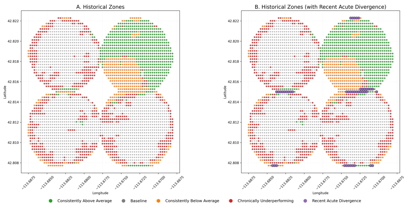
Figure 1. Sub-field biophysical regime maps derived from the K-Means clustering framework. (A) Historical zone classification based on long-term monthly relET indicators (μrelET, σrelET, Ptemp). (B) Historical zones with the Recent Acute Divergence overlay (purple), revealing acute anomalies during the 2025 growing season.
Informatics 13 00095 g001
Figure 2. Signal directionality map showing the spatial distribution of cross-methodological agreement and contradiction for the 869 pixels where both methods detected a persistent anomaly. Green: both methods agree on Consistently High; Orange: both agree on Consistently Low; Red: the methods assign opposite directions (contradiction).
Informatics 13 00095 g002
Figure 3. Three-panel cross-methodological validation. (A) Legacy persistence baseline derived from 16-year seasonal total ET in previous study [10], corresponding to Figure 7c of Reference [10]: persistently high (green), persistently low (blue), and baseline (gray). (B) Unsupervised K-Means zonation from the current framework. Classified categories are intentionally color-coded to be comparable to previous study. (C) Spatial distribution of agreement status: green = Validated High, blue = Validated Low, gray = Contradiction, orange = AI Downgrade to True Baseline.
Informatics 13 00095 g003
Figure 4. Statistical corroboration of cross-algorithmic agreement classes using paired t-tests on seasonal total ET (α = 0.05), evaluated against the true field-average ET computed from all pixels. Bars show the proportion of pixels in each class that are statistically significantly different from the field mean (green) versus not significantly different (gray). The AI-downgraded class is dominated by non-significant pixels (95.3%), indicating a lack of consistent multi-year deviation from field-average behavior, while validated low-performing zones retain strong statistical separation.
Informatics 13 00095 g004
Figure 5. Physical verification of algorithmic classifications via seasonal total evapotranspiration. (A) Raw seasonal total ET distributions for Validated High, AI Downgrade, Validated Low, and Field Average pixel populations. The downgraded population overlaps closely with the field average median. (B) ET residuals (Pixel ET minus Field Average ET). The AI Downgrade population is tightly centered on zero, confirming physical collapse into the field mean, while the Validated Low population maintains a clear negative offset. Boxplot colors correspond to the subfield regions shown in Figure 3.
Informatics 13 00095 g005
Figure 6. Kernel Density Estimation (KDE) of seasonal total ET residuals. (A) Pixel ET vs. field-average ET scatter plot: Validated High pixels cluster above the 1:1 line; Validated Low below; AI Downgrade pixels straddle it. (B) KDE of ET differences: the AI Downgrade density (orange) peaks at zero difference, providing visual corroboration that 95.3% of these pixels are statistically indistinguishable from the field mean.
Informatics 13 00095 g006
Figure 7. Zero-shot counterfactual validation of the five K-Means biophysical regimes. Representative pixel time series for each cluster showing monthly relET from 2000 to 2025 (black line), the model’s median counterfactual expectation for the 2025 growing season (dashed blue), the 80% prediction interval (shaded blue), and observed 2025 values (colored diamonds). Panels (AD): stable regimes where observed behavior closely tracks the counterfactual expectation. Panel (E): Recent Acute Divergence, where observed behavior falls entirely outside the counterfactual envelope, indicating a sudden system-state disruption, not chronic constraint.
Informatics 13 00095 g007
Table 1. Confusion matrix for directional agreement between the K-Means pipeline and legacy persistence baseline on the 869 shared-signal pixels.
Legacy: HighLegacy: LowRow Total
ML: High30495399
ML: Low26444470
Column Total330539869
Table 2. Cross-methodological agreement statistics and per-field breakdown for shared-signal pixels (n = 869). Results are reported separately for the four study fields: the northwest field (Field 39), northeast center-pivot field (Field 42), southwest field (Field 26), and southeast field (Field 27).
FieldShared PixelsBoth LowBoth HighAccuracy (%)Cohen’s κ
261441081081.90.336
27146108678.10.163
39168112469.00.038
4241111628497.30.936
All86944430486.10.716
Disclaimer/Publisher’s Note: The statements, opinions and data contained in all publications are solely those of the individual author(s) and contributor(s) and not of MDPI and/or the editor(s). MDPI and/or the editor(s) disclaim responsibility for any injury to people or property resulting from any ideas, methods, instructions or products referred to in the content.