Abstract
The growing sophistication of cyberattacks in Internet of Things (IoT) environments demands proactive and efficient solutions. We present an automated hyperparameter optimization (HPO) method for detecting cyberattacks in IoT that explicitly addresses class imbalance. The approach combines a Random Forest surrogate, a UCB acquisition function with controlled exploration, and an objective function that maximizes weighted F1 and MCC; it also integrates stratified validation and a compact selection of descriptors by metaheuristic consensus. Five models (RandomForest, AdaBoost, DecisionTree, XGBoost, and MLP) were evaluated on CICIoT2023 and CIC-DDoS2019. The results show systematic improvements over default configurations and competitiveness compared to Hyperopt and GridSearch. For RandomForest, marked increases were observed in CIC-DDoS2019 (F1-Score from 0.9469 to 0.9995; MCC from 0.9284 to 0.9986) and consistent improvements in CICIoT2023 (F1-Score from 0.9947 to 0.9954; MCC from 0.9885 to 0.9896), while maintaining low inference times. These results demonstrate that the proposed HPO offers a solid balance between performance, computational cost, and traceability, and constitutes a reproducible alternative for strengthening cybersecurity mechanisms in IoT environments with limited resources.
1. Introduction
Machine learning (ML) is transforming a wide range of industries through its application in fields such as medical diagnosis [1,2,3,4], education [5], autonomous vehicles [6,7], and finance [8], among others [9]. However, the performance of ML models depends heavily on the configuration of their hyperparameters, a process known as hyperparameter optimization (HPO) or tuning. Hyperparameters are settings that govern the model’s learning process and must be defined before training [10]. This includes hyperparameters such as the learning rate, the depth of decision trees, or the architecture of neural networks [11,12,13]. For example, the RandomForest implementation in Scikit-Learn has 19 hyperparameters that must be carefully defined before implementation [14].
These hyperparameters can be configured in various ways, depending on the model and dataset. One approach is manual tuning through trial and error. However, this process is time-consuming, resource-intensive, and highly dependent on the researcher’s experience, with no guarantee of finding an optimal configuration, especially for complex models with high-dimensional hyperparameter spaces [15,16]. On the other hand, using the default values provided by ML libraries offers a convenient starting point. However, these default values are rarely tailored to a specific problem or dataset and may therefore compromise model performance [17].
To address these limitations, various automated and systematic HPO methods have been developed. Among them, Grid Search (GS) exhaustively evaluates all combinations within a pre-defined parameter space [18]. In practice, an iterative procedure is often used to approximate a global optimum: the search begins with a broad range of values and a large step size, then progressively refines the search around promising regions based on the results. Although straightforward to implement, its main disadvantage is its inefficiency in high-dimensional spaces, as the number of evaluations grows exponentially with the number of hyperparameters, a phenomenon known as the curse of dimensionality [19]. Formally, for parameters each taking distinct values, the computational complexity scales as [20]. Consequently, GS is only effective for small configuration spaces.
Another technique is Random Search (RS), which has a very similar approach to GS, proposing to randomly sample a predefined number of values from the space between the upper and lower limits as candidate hyperparameter values, and then train each of these candidates [21]. It should be noted that if the value space is large enough, it can identify the global optimum or approximations, and with a limited budget it explores more regions than GS. This technique easily parallelizes and allocates resources because each evaluation is independent; since the total number of evaluations n is fixed before starting, its complexity is [22]. By sampling from a specified distribution, it reduces the risk of investing time in low-performing subregions and, with sufficient budget, can find the optimum or near-optimum.
Bayesian optimization (BO) is an iterative method for HPO that, unlike GS and RS, decides each new evaluation based on previous results using a probabilistic surrogate model and an acquisition function [23]; the surrogate estimates the posterior distribution of performance, and the acquisition selects points that balance exploration and exploitation to maximize the probability of identifying the global optimum or its best approximation, avoiding overlooking superior configurations in unexplored areas. Its operating cycle is: build the surrogate, propose the optimal configuration in the model, evaluate it in the actual objective function, update the surrogate, and repeat until the iteration limit is reached.
A very popular HPO library is Hyperopt, which implements a sequential optimization process guided by surrogates such as the tree-structured Parzen estimator (TPE) [24]. It formalizes the search as an acyclic expression graph where a null distribution of space is defined (specification language with stochastic nodes and choice for conditional parameters), a loss function, an optimization algorithm, and a database that accumulates the history of configurations and losses; its core is TPE, which learns two densities on each hyperparameter, for the best configurations and for the rest (modeled with Gaussian mixtures), and proposes new candidates by maximizing , a strategy equivalent to optimizing a form of expected improvement but more suitable for mixed and hierarchical domains [25].
Detecting attacks on IoT poses specific challenges for HPO, and even more so due to the vulnerabilities of IoT devices, such as the heterogeneity of communication protocols, low computing power, irregular update cycles, among others [26,27]. This has led to the emergence of different types of attacks such as distributed denial of service (DDoS), malware, botnets, etc. [28]. To address these threats, different ML models are implemented that are trained with datasets that present a severe imbalance between normal traffic and certain types of attacks, which skew metrics such as accuracy and require optimizing more informative objectives such as weighted F1, AUC-ROC/PR, and MCC [29,30,31].
In previous studies [32,33,34,35,36], it has been observed that hyperparameter optimization has been carried out arbitrarily or has not been detailed systematically. This often translates into combinations of default values, manual adjustments, weak validation protocols, inadequate metrics in the face of imbalance, and the absence of cross-validation, generating optimistic and poorly reproducible estimates. To address these limitations, we propose a hyperparameter optimization method geared toward detecting cyberattacks in IoT, structured in four stages: (i) a robust surrogate based on Random Forest; (ii) an Upper Confidence Bound (UCB) acquisition function that balances exploration and exploitation of the search space; (iii) an early stopping scheme to reduce computational cost; and (iv) a multi-objective criterion that maximizes weighted F1 and normalized MCC, with soft constraints on latency and model size.
The proposed method is compared with Hyperopt, GridSearch and evaluated on five supervised learning models, each with specific hyperparameter spaces. To accelerate training and inference, heuristic optimizers such as Adaptive Aquila Optimizer (AAO), Artificial Bee Colony (ABC), Ant Colony Optimization (ACO), Adaptive Inertia Weight Particle Swarm Optimization (AIW-PSO), and Hybrid Improved Whale Optimization Algorithm (HI-WOA) were integrated. Through consensus among heuristics, the most relevant characteristics of the datasets are identified. The evaluation was performed on CICIoT2023 and CIC-DDoS2019, aimed at threat classification in IoT environments with limited resources. The experimental results show significant improvements in attack detection for the optimized ML models compared to their non-optimized counterparts.
Within this framework, the research aligns with the Sustainable Development Goals (SDGs). It contributes to SDG 9 (Industry, Innovation, and Infrastructure) by offering an interoperable and reproducible HPO scheme that optimizes ML models for IoT devices with limited resources. Thus, the study not only advances the state of the art in IoT threat detection with rigorous evaluation and comparable protocols but also bridges the implementation gap by delivering a usable and standardizable HPO framework for edge and cloud deployments.
2. Methodology
2.1. Materials
For this study, two datasets were used to evaluate the performance of the proposed HPO method together with five ML models for classifying IoT attacks. The CICIoT2023 dataset [37] provides a realistic representation of 33 types of attacks grouped into 8 categories, including normal traffic: DDoS, DoS, reconnaissance, web, brute force, impersonation, and Mirai. It features a total of 46,686,579 records and 47 descriptors, obtained from the original PCAP files. The second dataset was CIC-DDoS2019 [38], specifically aimed at characterizing malicious traffic from 17 types of DDoS attacks, with 431,371 records and 80 descriptors. This dataset complements the first by offering a more DDoS-focused perspective, which allowed us to analyze the performance of the models in scenarios with different volumes and attribute granularities. Both datasets were selected to ensure diversity of scenarios and realism in the tests, allowing us to evaluate the generalization capacity of the proposed classifiers.
The proposed method and classification algorithms were implemented using the Python 3.12.7 programming language and various ML libraries such as Scikit-learn and Mealpy, among others. The calculations were performed on a computer equipped with an Intel Core Ultra 9 275HX processor, 32 GB of RAM, NVIDIA GeForce RTX 5080 GPU, and Windows 11 64-bit operating system.
2.2. Data Preprocessing, Standardization, and Division
Data preprocessing is considered one of the most important and critical steps before implementing an ML model. The following steps were applied:
- -
- Initially, given the large number of records in the CICIoT2023 dataset (approximately 46 million records), it was decided to implement a stratified subsampling of 1% in all classes, resulting in a dataset of 466,846 records. This decision was based on the fact that it ensures that the proportion of the attack class and the benign class is maintained, preserving the original distribution and the nature of the imbalance problem. The global seed used was 42, which is used for both subsampling and stratified cross-validation. All compared methods share exactly the same folds in order to perform paired comparisons. The evaluation protocol is based on k-fold cross-validation (k = 10); in each fold, preprocessing is adjusted exclusively with the training data from the fold to avoid data leakage. In the CIC-DDoS2019 dataset, which contained 431,371 records, 100% of the records were used, maintaining the same criteria as for the first dataset used.
- -
- Descriptors with constant values in all records were analyzed and removed from the datasets to optimize the analysis. In the CICIoT2023 dataset, six descriptors were identified that met this condition, namely: ‘ece_flag_number’, ‘cwr_flag_number’, ‘Telnet’, ‘SMTP’, ‘IRC’, and ‘DHCP’. In the CIC-DDoS2019 dataset, twelve descriptors with constant values were identified: ‘Bwd PSH Flags’, ‘Fwd URG Flags’, ‘Bwd URG Flags’, ‘FIN Flag Count’, ‘PSH Flag Count’, ‘ECE Flag Count’, ‘Fwd Avg Bytes/Bulk’, ‘Fwd Avg Packets/Bulk’, ‘Fwd Avg Bulk Rate’, ‘Bwd Avg Bytes/Bulk’, ‘Bwd Avg Packets/Bulk’, and ‘Bwd Avg Bulk Rate’. In addition, the ‘Unnamed: 0’ descriptor containing the sequential numbering of the records was removed, as was the ‘Label’ descriptor that included the type of attack for each record. It was also decided to remove this because there was another descriptor, ‘Class’, that grouped the different types of attacks more appropriately. At this stage, 6 descriptors from CICIoT2023 and 14 descriptors from CIC-DDoS2019 were removed.
- -
- An analysis of duplicate, empty, and infinite values (positive and negative) was also performed to identify and remove them from the datasets. In the case of CICIoT2023, no records were found that met these conditions. In contrast, 7698 duplicate records were identified in CIC-DDoS2019, which were removed to ensure the quality of the information analyzed.
- -
- Standardizing (z-score) the data allows the algorithms to generalize much better and more stable. For each descriptor, we compute the mean and standard deviation on the training split only and apply the same parameters to validation and test.
- -
- The new preprocessed dataset is divided into training, validation, and test sets with a ratio of 60%, 20%, and 20%, respectively, using a fixed random seed (42) to preserve class priors. The division was performed in a stratified manner, ensuring that the proportion of each class remained constant across all subsets.
2.3. Feature Selection
A robust approach is established to select the most relevant characteristics of the datasets, which integrated five optimization algorithms: ACO, ABC, AAO, AIW_PSO, HI-WOA. To balance consensus and diversity, only descriptors selected by at least three of the five algorithms are retained. An objective function was established to automatically evaluate the quality of each subset of features proposed by the optimization algorithms. For each candidate solution, a binary mask is constructed from a threshold of 0.5 indicating which attributes are included in the model. With the selected features, a Decision Tree is trained using the training set and predictions are made on the test set. Subsequently, two complementary metrics (F1 Score and Matthews Correlation Coefficient (MCC)) are calculated and combined using their geometric means to obtain a single fitness value. This approach allows for the simultaneous measurement of classifier performance and stability, favoring the selection of more informative features for IoT attack detection.
Taking the study proposed in [39] as a reference, Algorithm 1 is presented, which describes the feature selection process.
| Algorithm 1: Feature Selection Process | |
| 1. | Step 1: Load dataset and optimization algorithms |
| 2. | Import CICIoT2023, CIC-DDoS2019. |
| 3. | |
| 4. | Step 2: Define the fitness function |
| 5. | Use a DecisionTree (DT) as the base model |
| 6. | Evaluate performance on the validation set using the geometric mean between |
| 7. | F1 Score and MCC. |
| 8. | Step 3: Run optimization algorithms |
| 9. | : |
| 10. | using DT. |
| 11. | Record the best binary mask. |
| 12. | End |
| 13. | Step 4: Add Feature Selection Results |
| 14. | Step 5: Output |
| 15. | Return to the final list of features selected by at least three optimization algorithms |
2.4. Proposed HPO Method
The HPO problem consists of finding a hyperparameter configuration within a search space that maximizes the performance of an ML model, measured by an objective function . Formally, it can be expressed as [16]:
where is the hyperparameter configuration that produces the optimal value , and a hyperparameter can take any value from the search space , which can be continuous, integer, or categorical values. Since is computationally expensive, sequential optimization with a surrogate is used.
The concept of surrogate is not new; it is the basis of the Bayesian optimization method that integrates SMAC (Sequential Model-based Algorithm Configuration) [40]. In SMAC, a Gaussian model is defined, where and are the mean and variance of a regression function , estimated as , y . In this case, is the set of regression trees in the forest: each tree is trained by sampling with replacement instances from the training set, and in each tree, the partition nodes are chosen from hyperparameters, setting minimum thresholds for instances and the total number of trees to contain the cost. Among its limitations, it does not incorporate early stopping or adaptive capping, which can degrade performance with large time limits; its evaluations are restricted to small captimes and, when adding capping, the model must handle censored data; its convergence guarantees apply mainly to finite spaces (not to continuous parameters without additional smoothness assumptions); and the selection of configurations is based on a simple heuristic (multi-start local search and random sampling) that the authors themselves consider improvable when seeking diversity with high expected gain [40].
The methodological proposal does not seek to introduce a new optimization paradigm but rather positions itself as a highly specialized and effective variant of Bayesian Optimization (BO). Although the use of a Random Forest surrogate model to guide the search is a fundamental concept in approaches such as SMAC, the novelty lies in the combination of refinements specific to the domain of cybersecurity in IoT. These key improvements include a scalar objective function that explicitly maximizes the F1-Score and Matthews Correlation Coefficient (MCC) to handle class imbalance [30], a UCB acquisition function with an ε-greedy scheme and elite-guided mutation for more efficient space exploration, and the integration of an early stopping scheme to reduce computational costs. This combination, designed for the attack detection problem, is the main contribution of the study. Mathematically, it is expressed as:
- (i)
- Scalar objective function (weighted F1 + normalized MCC)
Let be the support-weighted over class and let , denote de multiclass Mathews correlation coefficient. We normalize to , as:
We combined and with the harmonic mean, adding a small stabilization constant (we use ):
For set of hyperparameters , the HPO objective is:
- (ii)
- Surrogate-based acquisition.
Let be an encoding of the hyperparameter vector . We fit a RandomForest surrogate on the archive , where is the size of the evaluations file in iteration ; . Denote the ensemble trees by , where is the total number of trees in the random forest. For any candidate , the surrogate mean and dispersion are:
We then score candidates with an upper confidence bound (UCB),
which trades off exploitation (large ) and exploration (large ).
- (iii)
- Candidate set and ε-greedy selection with elite-guided mutation
At iteration , we generate a pool , where is the number of candidates generated in iteration and indexes each candidate. The pool is built by random sampling from the search space and elite-guided mutation of the top-K configuration with highest rewards:
where controls mutation intensity and respects the constraints of each hyperparameter type integer, log-scaled, categorical or nullable. To avoid resampling, a canonical signature is used to filter duplicates. Selection follows ε-greedy police over UCB:
with a linear cooling schedule:
Early stopping. We terminate the search when no candidate surpasses the incumbent (best-so-far) reward by at least for consecutive iterations. Let be the scalar reward at iteration and the incumbent at iteration . We stop at iteration if,
That is, the improvement over the last iterations does not exceed . In all experiments we set , con iterations. This criterion operates on the incumbent (best-so-far) rather than on a running average.
- (iv)
- Stratified K-fold evaluation in parallel
Each is scored by stratified K-fold cross-validation to stabilize the estimate of
This reduces variance roughly as . Executing the folds over workers shorten wall-time to while keeping total work.
- (v)
- Computational complexity
Per iteration , fitting de RF surrogate over archive points costs with trees. Scoring candidates via UCB cost . Evaluating a chosen with k-fold CV cost , where is the model-specific training cost. Thus, the dominant term is per evaluation; total search cost scales with the matched budget .
As explained above, this approach is a specialized variant in the domain of optimization with a random forest surrogate, but it differs in three design options tailored to IoT cybersecurity. (i) We optimize a scalar objective that considers class imbalance, the support-weighted harmonic mean of F1 and a normalized MCC (Equations (3)–(5)), which prioritizes robust detection of minority classes. (ii) Candidate selection combines UCB acquisition with an ε-greedy policy and elite-guided mutation to maintain controlled diversity in mixed/hierarchical hyperparameter spaces (Equations (6)–(10)). (iii) We apply stratified K-fold evaluation with a tolerance-based early stopping rule (Equation (11)) to reduce computation and stabilize estimates (Equation (12)). Compared to SMAC, although both are based on RF surrogates, our method employs a different proposal policy (UCB + ε-greedy + elite mutation) and explicit F1/MCC scaling targeting severe imbalances, while BOHB focuses on multi-fidelity resource allocation through successive halving/Hyperband.
Method Calibration and Parameter Fixing
An experiment was designed on a synthetic multi-class dataset consisting of 100,000 records, 30 descriptors, and a category containing five classes. The classifier used in these tests is DecisionTree, and the space to be optimized was: max_depth ∈ {3, 150} or None (p = 0.25), min_samples_split ∈ {2, 30}, min_samples_leaf ∈ {1, 10}, ccp_alpha ∈ {1 × 10⁻⁶, 1 × 10⁻¹} (log), max_leaf_nodes ∈ {2, 50}, criterion ∈ {gini, entropy, log_loss}, and splitter ∈ {best, random}. This design covers everything from compact, regularized trees to deeper structures, maintaining stable encoding for the surrogate.
Table 1 shows five combinations of hyperparameters for the proposed method, covering exploration and exploitation scenarios. C1 (stable exploration) presents a balance between exploration and exploitation at a moderate cost. C2 (high exploration) presents greater space coverage, more variance, and time. C3 (high exploitation) presents convergence with risks of local optima. C4 (stable exploitation) is used to obtain more robust metrics with a higher cost per evaluation. C5 (intensive optimization) is used to maximize the probability of achieving better rewards.

Table 1.
Hyperparameter combinations for the proposed HPO method.
The experimental results of the proposed method (Figure 1) show that F1, MCC, and harmonic reward evolve in tandem, with initial oscillations and subsequent stabilization in a narrow range between 0.863 and 0.868, suggesting that the tree’s hyperparameter space is relatively optimal for this problem. C1 offers a cost-performance balance with 0.863; by increasing exploration in C2 (higher ε and κ, more candidates and initiators), a slight increase in the maximum (≈0.866) is observed in exchange for greater variance and time; C3 (aggressive exploitation) converges quickly and cheaply but does not outperform C1, evidencing the risk of local optima; C4 (same dynamics as C1, but with CV = 5) smooths the signal and slightly increases robustness and the peak to 0.8665 with almost linear cost in folds; and C5 (intensive optimization, many iterations, large batch, and CV = 10) achieves the best value, reaching 0.8683 with the most stable signal at the end, although it is the most expensive option. In summary, more exploration tends to yield slightly better but more unstable peaks, more exploitation accelerates convergence with the risk of stagnation, and more CV improves reliability at a higher cost; given that the absolute differences are small, the choice should be guided by budget and risk tolerance.
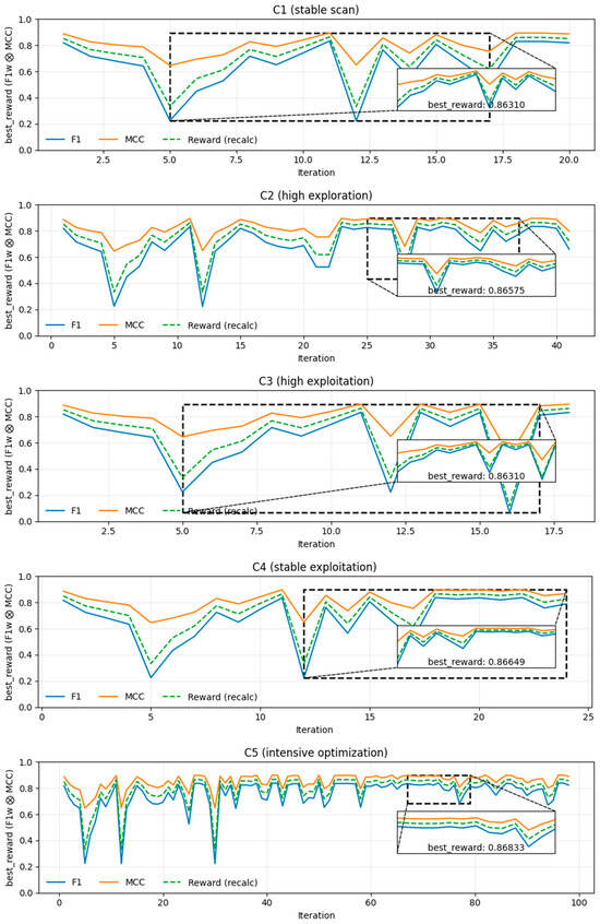
Figure 1.
Evolution of metrics and best reward under five HPO configurations (C1–C5) in synthetic dataset. The dashed rectangles in each main panel highlight the range of iterations in which the current best solution appears, while the solid rectangles frame the corresponding enlarged boxes that magnify this region and report the best reward value.
2.5. Evaluation Metrics for ML Models
Performance metrics are essential for evaluating the effectiveness of an ML model, and the confusion matrix is the starting point for this analysis. By comparing predictions with actual labels, the matrix allows us to quantify hits and misses by class and obtain key indicators: accuracy expresses the proportion of correct predictions; the F1 score combines precision and recall into a single useful measure when it is necessary to balance both aspects; and the MCC or Matthews correlation coefficient summarizes the quality of the classification by taking into account true and false positives/negatives. Together, these metrics provide a more comprehensive and reliable view of performance, especially valuable in multi-class or class-imbalanced scenarios, where precision alone can be misleading. All of these metrics are derived from the confusion matrix, where TP corresponds to true positives, TN to true negatives, FP to false positives, and FN to false negatives.
3. Results
3.1. Selection of Descriptors
The selection of descriptors combined five heuristic algorithms (AAO, ABC, ACO, AIW_PSO, HI_WOA), retaining descriptors for at least three algorithms, ensuring consensus and diversity. To evaluate the suitability of the heuristic algorithms, the study in [39] was used as a reference, which implemented a decision tree optimized using the geometric mean F1 and MCC to balance precision and recall. This improved predictive performance by prioritizing the most relevant features, increasing the efficiency of detecting different attacks on IoT. Table 2 consolidates the results of the selected descriptors. For CICIoT2023, timing and traffic header descriptors predominated, while for CIC-DDoS2019, packet lengths/rates and transport flags predominated.
Table 2.
Summary of feature selection by dataset and consensus frequency.
3.2. Results Without Hyperparameter Tuning
Five classifiers were implemented: RandomForest (RF), Adaboost (ADA), DecisionTree (DT), XGBoost (XGB), and Multilayer Perceptron (MLP), using the default values specified in the scikit-learn library [41]. Table 3 shows the performance metrics for the two datasets used. For the CICIoT2023 dataset, RF exhibited the best initial performance with an F1-Score of 0.994740 and an MCC of 0.988533. The DT and XGB models showed statistically close results, with F1-Score values of 0.993787 and 0.993566, respectively. In the case of the CIC-DDoS2019 dataset, RF again ranked as the best starting point (F1-Score: 0.946909, MCC: 0.928399), with DT (F1-Score: 0.946506) and XGB (F1-Score: 0.945887) as competitive alternatives. In terms of efficiency, DT had the shortest inference time in both scenarios (0.013083 s for CICIoT2023 and 0.010000 s for CIC-DDoS2019), which shows a favorable result between predictive performance and computational cost compared to more complex models such as RF.
Table 3.
Performance metrics without hyperparameter tuning.
3.3. Results with Hyperparameter Tuning
The tuning results of the proposed method and Hyperopt are reported. Although GridSearch is widely used, its exhaustive execution over the same search space was computationally unfeasible; for example, in DecisionTree it took over 14,400 s to find the best hyperparameters. For this reason, complete GridSearch results are not included, and the analysis focuses on the detailed results of the proposed method and Hyperopt. In the case of Hyperopt, stratified cross-validation (k = 10) and 20 evaluations per search were used. The proposed method was run with the C5 configuration (Section Method Calibration and Parameter Fixing). The initial ranges of the hyperparameters were set randomly; then, preliminary tuning was performed with Hyperopt on a subset of data from the training set. When the average best score was <0.98, the value ranges were expanded or shortened, and the search was repeated until that threshold was exceeded.
With the search space now stabilized, optimization was performed on the entire training set (60%) and the model was trained using training + validation (80%). The final evaluation was performed on the test set (20%), which was not used during optimization. For the datasets used, the final ranges and selected values are summarized in Table 4.
Table 4.
Definition of the value space for ML models.
For the CICIoT2023 dataset (Table 5), the proposed method demonstrates significant improvements in efficiency and performance for certain models. In the case of RF, it reduces training time by 77.1% at the cost of a minimal decrease in score (−0.000307). For ADA and DT, it not only improves the score (+0.002858 and +0.010278, respectively) but also shortens training times by 33.9% and 45.8%. On the other hand, Hyperopt maintains an advantage in the score for XGB (+0.000644) and MLP (+0.001234), although this implies a higher time cost in the case of XGB.
Table 5.
Obtaining the best hyperparameters for the CICIoT2023 dataset.
In the analysis of the CIC-DDoS2019 dataset (Table 6), similar patterns are observed. The proposed method outperforms Hyperopt in RF (+0.000033) and DT (+0.003706) scores, also achieving training time reductions of 68.4% and 32.0%, respectively. For ADA, although Hyperopt achieves a higher score (+0.000881), the proposed method is considerably faster (59.9%). Hyperopt remains marginally superior in score for XGB (+0.000356) and MLP (+0.000645), with variable training times.
Table 6.
Obtaining the best hyperparameters for the CIC-DDoS2019 dataset.
Table 7 consolidate the final metrics of the optimized models in the test sets. Key findings reveal that the proposed method achieves the most substantial performance gain with the DT model in the CICIoT2023 dataset, increasing the MCC by 0.024301 compared to Hyperopt while reducing inference time. Similarly, for the CIC-DDoS2019 dataset, the proposed method consistently improves the performance of RF and DT, with a notable increase in the MCC of DT, which goes from 0.98461 to 0.995703. In addition, the proposed method demonstrates a remarkable ability to reduce inference times without sacrificing performance; for example, with RF on CIC-DDoS2019, it achieves a higher F1-Score with an inference time 19.7% lower. Hyperopt maintains a marginal advantage in score for MLP models in both datasets and for XGB in CIC-DDoS2019, although the differences are minimal. Finally, the ADA classifier optimized with the proposed method for CICIoT2023 shows a significant improvement in MCC (+0.009705), consolidating itself as a robust alternative.
Table 7.
Performance metric results for the CICIoT2023 and CIC-DDoS2019 datasets.
The comparison between the results with default values (Table 3) and those obtained after hyperparameter optimization (Table 7) confirms the importance of the HPO phase. Although the base models already showed high performance, systematic adjustment consistently increased accuracy, F1-Score, and MCC, with particular emphasis on CIC-DDoS2019, where classifiers such as RF and DT went from a range of approximately 0.92–0.94 to higher values of 0.99 in F1/MCC. In CICIoT2023, the improvements were more moderate but uniform across methods, suggesting that HPO not only increases the average level of performance but also reduces variability between configurations. Furthermore, these benefits are achieved without significantly penalizing inference times, maintaining viability in resource-constrained environments. This demonstrates that optimization is not a marginal improvement, but a fundamental step in unlocking the maximum predictive potential of classifiers and ensuring robust, high-fidelity attack detection capabilities.
Another relevant aspect is the tuning time required by each HPO method. In several cases (for example, RF and DT), the proposed method achieves better or equivalent “best scores” with less training time, suggesting more efficient exploration of the space and early convergence toward promising regions (local quality optima). This time advantage is especially visible in CICIoT2023 (see Table 5 and Table 6), where the reduction in the time needed to find competitive configurations is systematic without sacrificing stability or metrics. Overall, the results indicate that, in addition to improving performance, the proposed search scheme optimizes computational cost, a critical factor for limited budgets and IoT/edge scenarios.
Table 8 presents a comparative analysis of the results of this study with recent work in the literature on IoT cybersecurity. However, it is important to note that a direct comparison is inherently difficult due to differences in evaluation protocols, datasets, and reported metrics. Specifically, the reference works use different benchmarks (e.g., BOTIoT, TON-IoT [32], and MBB-IoT [35,36]), employ a variable number of descriptors, and do not consistently report the F1-Score and MCC, metrics that are critical for imbalanced datasets, as well as HPO techniques. This means that comparisons should be read with caution and as indicative, not conclusive, evidence. Even so, Table 8 reveals clear patterns: several papers report accuracy (e.g., [35] 0.9998 in MBB-IoT) or F1 per class ([34]: 100% for DDoS and 97% for Benign), omitting global F1 and MCC; the number of descriptors varies widely (20–77); and HPO is rarely documented (only [34] mentions Random Search). In this context, our approach with transparently optimized RF achieves promising results in generalizing different types of attacks and is viable for deployment in IoT environments.
Table 8.
Comparative analysis of the proposed approach.
4. Conclusions
This paper presents a systematic, reproducible HPO method adapted to the challenges of cybersecurity data, such as class imbalance. Unlike arbitrary approaches documented in the literature, the method integrates a Random Forest surrogate, a controlled exploration UCB acquisition function, and an objective function that maximizes F1-Score and MCC to address imbalanced sets.
The results demonstrate that the HPO process is a fundamental step, rather than a merely marginal one, in maximizing the effectiveness of ML models in cybersecurity. Systematic optimization allowed us to raise the performance of the classifiers from an already robust base to a higher level of accuracy and reliability, with F1-Score and MCC metrics exceeding 0.99 in the complex CIC-DDoS2019 dataset. The most notable finding is the competitiveness of the proposed method compared to an established standard such as Hyperopt. This method not only matched or exceeded predictive performance in most scenarios, but also achieved dramatic reductions in training times, demonstrating a superior balance between computational efficiency and detection capability.
Although the feature selection approach based on metaheuristic consensus proved to be robust, it is important to recognize an inherent methodological limitation in the fitness function used. To evaluate the quality of the feature subsets, a Decision Tree was used as a reference model. This choice, while computationally efficient, introduces a non-trivial bias: the selected feature set is best suited for tree-based models (such as DT, RF, and XGB), but may not be optimal for classifiers with fundamentally different architectures, such as MLP. The results in the study, where the greatest performance gains are observed in tree models, could reflect this bias. As future work, we propose exploring the use of a model-agnostic fitness function or one based on a committee of classifiers, to obtain a more universally applicable subset of features, as well as deploying the adjusted models in a real-world setting with a tolerance scheme based on periodic re-tuning, sliding windows, and semi-supervised learning.
Author Contributions
Conceptualization, F.L.B.-S. and M.G.F.; data curation, formal analysis, Project administration, Software, Visualization, Writing—review and editing, F.L.B.-S.; Investigation, Resources, Validation, Writing—original draft, F.L.B.-S., L.P., M.J.G.-C., M.D. and M.G.F.; Methodology, F.L.B.-S., L.P. and M.G.F.; Supervision, F.L.B.-S. and M.G.F. All authors have read and agreed to the published version of the manuscript.
Funding
This work was developed thanks to the competitive grant for the multidisciplinary project “New methods based on machine learning for the detection of cyber-attacks in IoT environments,” approved by Resolution No. 098-2025-R-UPNW at Norbert Wiener Private University.
Institutional Review Board Statement
Not applicable.
Informed Consent Statement
Not applicable.
Data Availability Statement
The data may be provided free of charge to interested readers by requesting the correspondence author’s email.
Conflicts of Interest
The authors declare no conflicts of interest.
References
- García-García, R.E. Applications of Artificial Intelligence in Hospital Quality Management: A Review of Digital Strategies in Healthcare Settings. Rev. Cient. Sist. Inform. 2025, 5, e928. [Google Scholar] [CrossRef]
- Mahoto, N.A.; Shaikh, A.; Sulaiman, A.; Reshan, M.S.A.; Rajab, A.; Rajab, K. A Machine Learning Based Data Modeling for Medical Diagnosis. Biomed. Signal Process. Control 2023, 81, 104481. [Google Scholar] [CrossRef]
- Bolia, C.; Joshi, S. Optimized Deep Neural Network for High-Precision Psoriasis Classification from Dermoscopic Images. Rev. Cient. Sist. Inform. 2025, 5, e966. [Google Scholar] [CrossRef]
- Rodriguez, M.R.R.; Calpa, C.A.D.; Paz, H.A.M. Comparison of kernel functions in the prediction of cardiovascular disease in Artificial Neural Networks (ANN) and Support Vector Machines (SVM). EthAIca 2025, 4, 172. [Google Scholar] [CrossRef]
- Del-Águila-Castro, M. Sistemas Inteligentes y su Aplicación en la Evaluación del Desempeño Académico Universitario: Una Revisión de la Literatura en el Contexto Sudamericano. Rev. Cient. Sist. Inform. 2024, 4, e671. [Google Scholar] [CrossRef]
- Garikapati, D.; Shetiya, S.S. Autonomous Vehicles: Evolution of Artificial Intelligence and the Current Industry Landscape. Big Data Cogn. Comput. 2024, 8, 42. [Google Scholar] [CrossRef]
- Shafique, R.; Rustam, F.; Murtala, S.; Jurcut, A.D.; Choi, G.S. Advancing Autonomous Vehicle Safety: Machine Learning to Predict Sensor-Related Accident Severity. IEEE Access 2024, 12, 25933–25948. [Google Scholar] [CrossRef]
- El Hajj, M.; Hammoud, J. Unveiling the Influence of Artificial Intelligence and Machine Learning on Financial Markets. J. Risk Financ. Manag. 2023, 16, 434. [Google Scholar] [CrossRef]
- Melo, R.A.V.; Peña, J.C.C.; Rosero, J.A.R. Enriching the tourist experience at the Santuario de las Lajas through image recognition using WhatsApp. EthAIca 2025, 4, 180. [Google Scholar] [CrossRef]
- Raiaan, M.A.K.; Sakib, S.; Fahad, N.M.; Al Mamun, A.; Rahman, A.; Shatabda, S.; Mukta, S.H. A Systematic Review of Hyperparameter Optimization Techniques in Convolutional Neural Networks. Decis. Anal. J. 2024, 11, 100470. [Google Scholar] [CrossRef]
- Bischl, B.; Binder, M.; Lang, M.; Pielok, T.; Richter, J.; Coors, S.; Thomas, J.; Ullmann, T.; Becker, M.; Boulesteix, A.; et al. Hyperparameter Optimization: Foundations, Algorithms, Best Practices, and Open Challenges. WIREs Data Min. Knowl. Discov. 2023, 13, e1484. [Google Scholar] [CrossRef]
- Franceschi, L.; Donini, M.; Perrone, V.; Klein, A.; Archambeau, C.; Seeger, M.; Pontil, M.; Frasconi, P. Hyperparameter Optimization in Machine Learning. arXiv 2025. [Google Scholar] [CrossRef]
- Shekhar, S.; Bansode, A.; Salim, A. A Comparative Study of Hyper-Parameter Optimization Tools. In Proceedings of the 2021 IEEE Asia-Pacific Conference on Computer Science and Data Engineering (CSDE), Brisbane, Australia, 8–10 December 2021. [Google Scholar] [CrossRef]
- scikit-learn. RandomForestClassifier. Available online: https://scikit-learn.org/stable/modules/generated/sklearn.ensemble.RandomForestClassifier.html (accessed on 24 August 2025).
- Akinremi, B. Best Tools for Model Tuning and Hyperparameter Optimization. Neptune.ai. Available online: https://neptune.ai/blog/best-tools-for-model-tuning-and-hyperparameter-optimization (accessed on 24 August 2025).
- Yang, L.; Shami, A. On Hyperparameter Optimization of Machine Learning Algorithms: Theory and Practice. Neurocomputing 2020, 415, 295–316. [Google Scholar] [CrossRef]
- Elgeldawi, E.; Sayed, A.; Galal, A.R.; Zaki, A.M. Hyperparameter Tuning for Machine Learning Algorithms Used for Arabic Sentiment Analysis. Informatics 2021, 8, 79. [Google Scholar] [CrossRef]
- Injadat, M.; Moubayed, A.; Nassif, A.B.; Shami, A. Systematic Ensemble Model Selection Approach for Educational Data Zining. Knowl.-Based Syst. 2020, 200, 105992. [Google Scholar] [CrossRef]
- Claesen, M.; Simm, J.; Popovic, D.; Moreau, Y.; De Moor, B. Easy Hyperparameter Search Using Optunity. arXiv 2014. [Google Scholar] [CrossRef]
- Lorenzo, P.R.; Nalepa, J.; Kawulok, M.; Ramos, L.S.; Pastor, J.R. Particle Swarm Optimization for Hyper-Parameter Selection in Deep Neural Networks. In Proceedings of the Genetic and Evolutionary Computation Conference (GECCO ’17), Berlin, Germany, 15–19 July 2017; ACM: New York, NY, USA, 2017; pp. 481–488. [Google Scholar] [CrossRef]
- Bergstra, J.; Bengio, Y. Random Search for Hyper-Parameter Optimization. J. Mach. Learn. Res. 2012, 13, 281–305. [Google Scholar]
- Witt, C. Worst-Case and Average-Case Approximations by Simple Randomized Search Heuristics. In Proceedings of the 22nd Annual Conference on Theoretical Aspects of Computer Science (STACS’05), Stuttgart, Germany, 24–26 February 2005; Springer: Berlin/Heidelberg, Germany, 2005; pp. 44–56. [Google Scholar] [CrossRef]
- Snoek, J.; Larochelle, H.; Adams, R.P. Practical Bayesian Optimization of Machine Learning Algorithms. arXiv 2012. [Google Scholar] [CrossRef]
- Hyperopt Documentation. Available online: https://hyperopt.github.io/hyperopt/ (accessed on 17 September 2025).
- Bergstra, J.; Yamins, D.; Cox, D.D. Making a Science of Model Search: Hyperparameter Optimization in Hundreds of Dimensions for Vision Architectures. Proc. Mach. Learn. Res. 2013, 28, 115–123. [Google Scholar]
- Kumari, P.; Jain, A.K. A Comprehensive Study of DDoS Attacks over IoT Network and Their Countermeasures. Comput. Secur. 2023, 127, 103096. [Google Scholar] [CrossRef]
- Miri Kelaniki, S.; Komninos, N. A Study on IoT Device Authentication Using Artificial Intelligence. Sensors 2025, 25, 5809. [Google Scholar] [CrossRef]
- Wahab, S.A.; Sultana, S.; Tariq, N.; Mujahid, M.; Khan, J.A.; Mylonas, A. A Multi-Class Intrusion Detection System for DDoS Attacks in IoT Networks Using Deep Learning and Transformers. Sensors 2025, 25, 4845. [Google Scholar] [CrossRef]
- Saito, T.; Rehmsmeier, M. The Precision-Recall Plot Is More Informative than the ROC Plot When Evaluating Binary Classifiers on Imbalanced Datasets. PLoS ONE 2015, 10, e0118432. [Google Scholar] [CrossRef]
- Chicco, D.; Jurman, G. The Advantages of the Matthews Correlation Coefficient (MCC) over F1 Score and Accuracy in Binary Classification Evaluation. BMC Genom. 2020, 21, 6. [Google Scholar] [CrossRef]
- Davis, J.; Goadrich, M. The Relationship between Precision-Recall and ROC Curves. In Proceedings of the 23rd International Conference on Machine Learning (ICML ’06), Pittsburgh, PA, USA, 25–29 June 2006; ACM: New York, NY, USA, 2006; pp. 233–240. [Google Scholar] [CrossRef]
- Khanday, S.A.; Fatima, H.; Rakesh, N. Implementation of Intrusion Detection Model for DDoS Attacks in Lightweight IoT Networks. Expert Syst. Appl. 2023, 215, 119330. [Google Scholar] [CrossRef]
- Najar, A.A.; Manohar, N.S. A Robust DDoS Intrusion Detection System Using Convolutional Neural Network. Comput. Electr. Eng. 2024, 117, 109277. [Google Scholar] [CrossRef]
- Mahadik, S.S.; Pawar, P.M.; Muthalagu, R. Edge-HetIoT Defense against DDoS Attack Using Learning Techniques. Comput. Secur. 2023, 132, 103347. [Google Scholar] [CrossRef]
- Ullah, S.; Mahmood, Z.; Ali, N.; Ahmad, T.; Buriro, A. Machine Learning-Based Dynamic Attribute Selection Technique for DDoS Attack Classification in IoT Networks. Computers 2023, 12, 115. [Google Scholar] [CrossRef]
- Lv, H.; Du, Y.; Zhou, X.; Ni, W.; Ma, X. A Data Enhancement Algorithm for DDoS Attacks Using IoT. Sensors 2023, 23, 17496. [Google Scholar] [CrossRef]
- Neto, E.C.P.; Dadkhah, S.; Ferreira, R.; Zohourian, A.; Lu, R.; Ghorbani, A.A. CICIoT2023: A Real-Time Dataset and Benchmark for Large-Scale Attacks in IoT Environment. Sensors 2023, 23, 5941. [Google Scholar] [CrossRef]
- Sharafaldin, I.; Lashkari, A.H.; Hakak, S.; Ghorbani, A.A. Developing Realistic Distributed Denial of Service (DDoS) Attack Dataset and Taxonomy. In Proceedings of the 2019 International Carnahan Conference on Security Technology (ICCST), Chennai, India, 1–3 October 2019; pp. 1–8. [Google Scholar] [CrossRef]
- Akouhar, M.; Ouhssini, M.; El Fatini, M.; Abarda, A.; Agherrabi, E. Dynamic Oversampling-Driven Kolmogorov–Arnold Networks for Credit Card Fraud Detection: An Ensemble Approach to Robust Financial Security. Egypt. Inform. J. 2025, 31, 100712. [Google Scholar] [CrossRef]
- Hutter, F.; Hoos, H.H.; Leyton-Brown, K. Sequential Model-Based Optimization for General Algorithm Configuration. In Learning and Intelligent Optimization; Coello, C.A.C., Ed.; Springer: Berlin/Heidelberg, Germany, 2011; pp. 507–523. [Google Scholar] [CrossRef]
- scikit-learn: Machine Learning in Python—Scikit-Learn 1.7.2 Documentation. Available online: https://scikit-learn.org/stable/ (accessed on 18 August 2025).
Disclaimer/Publisher’s Note: The statements, opinions and data contained in all publications are solely those of the individual author(s) and contributor(s) and not of MDPI and/or the editor(s). MDPI and/or the editor(s) disclaim responsibility for any injury to people or property resulting from any ideas, methods, instructions or products referred to in the content. |
© 2025 by the authors. Licensee MDPI, Basel, Switzerland. This article is an open access article distributed under the terms and conditions of the Creative Commons Attribution (CC BY) license (https://creativecommons.org/licenses/by/4.0/).