Hybrid Approach Using Dynamic Mode Decomposition and Wavelet Scattering Transform for EEG-Based Seizure Classification

Abstract

Epilepsy is a brain disorder that affects individuals; hence, preemptive diagnosis is required. Accurate classification of seizures is critical to optimize the treatment of epilepsy. Patients with epilepsy are unable to lead normal lives due to the unpredictable nature of seizures. Thus, developing new methods to help these patients can significantly improve their quality of life and result in huge financial savings for the healthcare industry. This paper presents a hybrid method integrating dynamic mode decomposition (DMD) and wavelet scattering transform (WST) for EEG-based seizure analysis. DMD allows for the breakdown of EEG signals into modes that catch the dynamical structures present in the EEG. Then, WST is applied as it is invariant to time-warping and computes robust hierarchical features at different timescales. DMD-WST combination provides an in-depth multi-scale analysis of the temporal structures present within the EEG data. This process improves the representation quality for feature extraction, which can convey dynamic modes and multi-scale frequency information for improved classification performance. The proposed hybrid approach is validated with three datasets, namely the CHB-MIT PhysioNet dataset, the Bern Barcelona dataset, and the Khas dataset, which can accurately distinguish the seizure and non-seizure states. The proposed method performed classification using different machine learning and deep learning methods, including support vector machine, random forest, k-nearest neighbours, booster algorithm, and bagging. These models were compared in terms of accuracy, precision, sensitivity, Cohen’s kappa, and Matthew’s correlation coefficient. The DMD-WST approach achieved a maximum accuracy of 99% and F1 score of 0.99 on the CHB-MIT dataset, and obtained 100% accuracy and F1 score of 1.00 on both the Bern Barcelona and Khas datasets, outperforming existing methods

1. Introduction

Epilepsy is a cognitive impairment affecting millions of lives worldwide. This disorder significantly diminishes the standard of living of individuals diagnosed with it, published by [1]. Epilepsy can be caused by various factors, including genetic disorders, brain injury, infections, and developmental disorders. The treatment approaches include medications, lifestyle modifications, and in certain instances, surgical procedures. However, managing epilepsy can be challenging due to the multifaceted nature of the disorder. An electroencephalogram (EEG) is used to detect different brain activities. Early detection of epilepsy is important, as it can significantly impact the management and treatment of the condition. The occurrence of unprovoked seizures characterises epilepsy due to anomalies in the brain [2]. The seizures induce involuntary movements that may affect a portion or the entirety of the body, occasionally leading to disruptions in sensation, intellectual functioning, mood, or even loss of consciousness. seizures are distinguished into generalised seizures and focal seizures [3]. The frequency of seizures differs among patients, varying from less than once annually to many occurrences daily [4,5]. Detecting seizures through EEG signals is essential in diagnosing epilepsy [6]. Figure 1 and Figure 2 illustrate time series plots of signals during seizure and non-seizure files, respectively, for the CHBMIT dataset. Figure 3 and Figure 4 present representative EEG signal plots from the Barcelona and Khas datasets, respectively.

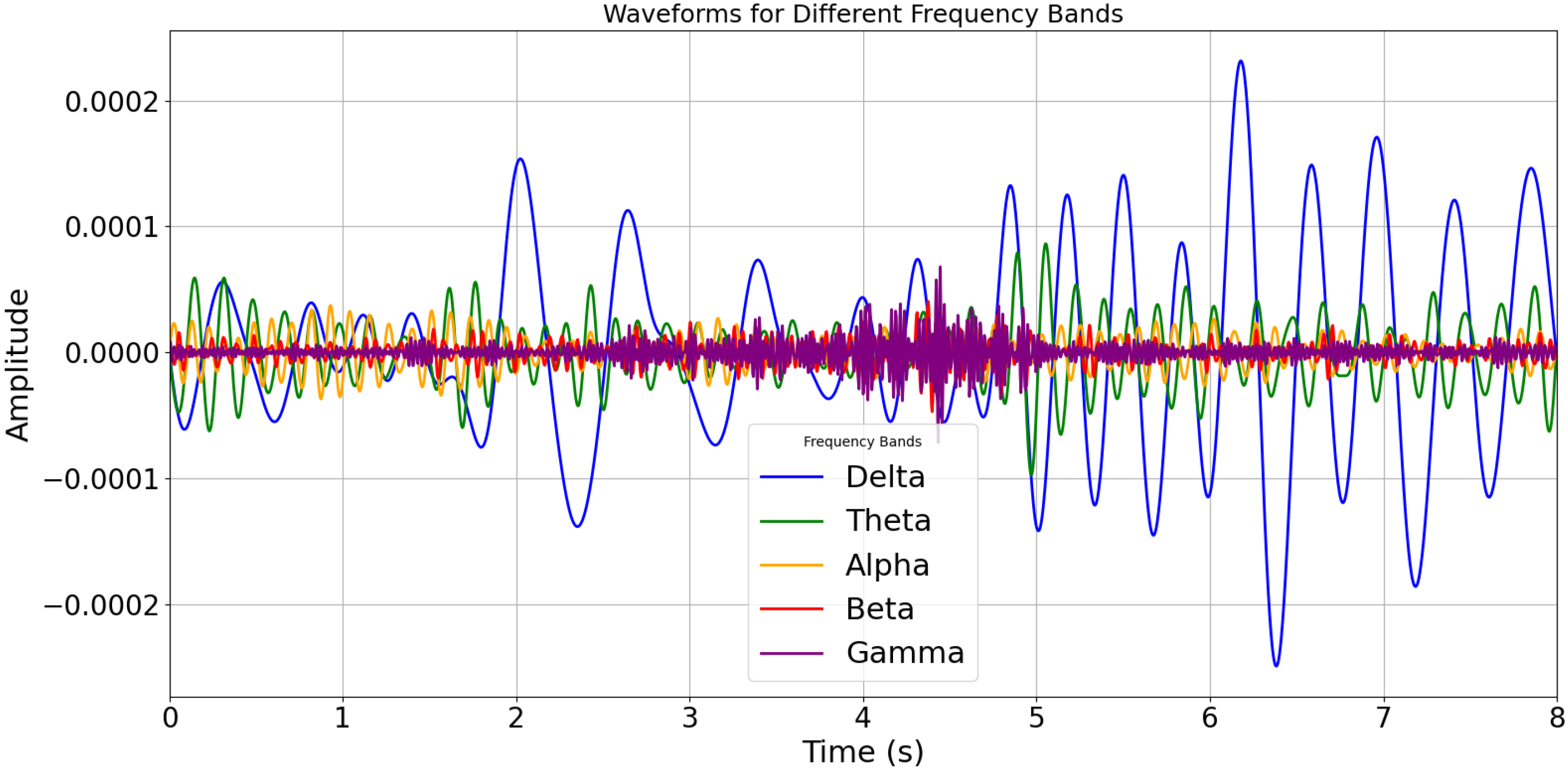
EEG signals related to seizures are organised into four stages based on the occurrence of a seizure, namely preictal, ictal, inter-ictal, and postictal. Preictal and postictal are the signal segments before and after the occurrences of seizures, respectively [7]. Inter-ictal refers to the irregular signal activities in the gaps between seizures, while ictal refers to the irregular signals present at the time of epileptic seizure. The characteristic of inter-ictal activities in EEG signals includes occasional transient waveforms. The EEG waveforms change in real time, dynamically increasing or decreasing their frequency and amplitude as the seizure spreads into different brain areas. EEG signals have different oscillatory modes, each associated with specific cognitive functions and mental states [3]. These are the sinusoids at different frequencies. Gamma waves are high-frequency brain waves during a highly alert and conscious state. The frequency range is from 30 to 70 Hz and is characterised by rapid oscillations. Beta waves are high-frequency brain waves (12–30 Hz) that are associated with cognitive activity, focus, critical thinking, and focused attention. alpha waves are lower-frequency brain waves (8–12 Hz) that are observed with relaxation and calmness. Theta waves (4–8 Hz) tend to occur with deep relaxation, light sleep, and meditation. Delta waves are the slowest brain waves seen in deep sleep (0.5–4 Hz). Figure 5 shows how these different frequency bands vary over time. Each EEG band captures distinct oscillatory activity, where delta illustrates slow and high-amplitude oscillations, theta/alpha shows medium frequency, and beta/gamma represents higher-frequency, lower-amplitude oscillations. This decomposition demonstrates that EEG signals in different frequency bands can be used in neurological applications such as the detection of seizures and classification.

Extensive research in recent years has focused on developing automatic epileptic seizure classification systems to aid in clinical practice by reducing the clinician’s workload and improving diagnosis [8,9]. Classification of seizure is an essential and challenging work because EEG signals can be of longer duration making it time-consuming to manually interpret and detect anomalies [10]. A variety of techniques is being explored to increase the efficiency of seizure classification. as a result, machine learning (ML) and deep learning (DL) algorithms are now considered essential tools, which offers promising solutions for improving the automatic diagnosis of epilepsy [4,5,11,12]. EEG data contains temporal, spatial, and spectral patterns crucial for diagnosing neurological disorders. Therefore, effective feature extraction is essential, as capturing these key patterns directly impacts the accuracy and efficiency of classification [13,14,15].

Understanding complex dynamic behaviour is critical in epilepsy classification, which demands the use of data-driven algorithms for accurate analysis. Dynamic mode decomposition (DMD) is a matrix factorization method specifically developed to analyse time-varying data, facilitating it ideal for EEG analysis by capturing the dynamic patterns and temporal evolution of seizure activity. This analysis effectively combines power spectral analysis in the temporal dimension with principal component analysis (PCA) in spatial [16,17]. In epilepsy studies, this approach offers a way to detect patterns of activity during seizures. Power spectral analysis detects abnormal rhythmic activity, such as sudden spikes in specific frequency bands. PCA highlights which areas of the brain demonstrate synchronised changes in activity during seizures. Together, they can help localise the brain areas from which seizures start and can show how seizures spread through the brain. Since conventional time- and frequency-domain features may not sufficiently characterise the fluctuations in EEG signals during seizures, wavelet transform-based analytical models are employed to extract deeper and more informative structures that enhance classification performance. Introduced by Mallet, [18] wavelet scattering transform (WST) is an optimally designed feature extractor for non-stationary signals. WST generates stable, accurate, and translation-invariant signal representations for EEG classification by effectively addressing signal deformations while maintaining class discriminability. Wavelet filters give high-frequency components, whereas scaling functions and local averages capture the low-frequency information. To alleviate information loss during averaging, high-frequency transforms can be reapplied to balance invariance and discriminability. Furthermore, combining WST and DMD supports thorough analysis of high-dimensional data, enhancing the extraction of features and understanding of complex behaviour.

The remaining sections are arranged as Section 2 explains the details of related work on EEG-based seizure analysis and Section 3 describes the details of the algorithms used in this study. Section 4 depicts the proposed methodology for seizure analysis and Section 5 evaluates the results of the proposed method. Section 6 discusses the validity of the results, and compares with the state-of-the-art to highlight its performance and the novelty of the hybrid method. Section 7 concludes the paper.

2. Related Works

Seizure classification is a challenging field of research when considering its goal to automatically classify epilepsy. The effectiveness of automatic seizure classification systems is influenced by feature extraction, which significantly affects the performance. This has prompted researchers to investigate a wide range of methodologies spanning multiple domains, including frequency, time, time-frequency, decomposition methods, and nonlinear approaches. In this section, the key scientific contributions and methodologies from prior studies that help for the advancement of EEG signal analysis are examined.

A prevalent technique for feature extraction is the Fourier transform (FT), yielding spectral information of the signal. Nevertheless, FT incorrectly assumes that the signal under investigation is stationary, whereas EEG signals are non-stationary. A further limitation of FT is its lack of timely information and not identifying exactly where an event occurs [19]. To address these challenges, short-time Fourier transform (STFT) has been used as a time-frequency analysis (TFA) technique. STFT divides a signal into time intervals with a short time window and applies the FT to analyse the signal within each interval. The major drawback of STFT is frequency and time resolution which cannot be simultaneously increased [20]. The window size in STFT remains unchanged throughout the analysis. Wide windows have good frequency resolution and narrow windows provide good time resolution. Hence, the choice of window width significantly affects the results. This problem in STFT is solved in wavelet transform (WT) by using wavelets. The multi-scale property of WT enables disassembling a signal into a set of scales where each scale captures a different level of coarseness associated with the analysed signal [21]. Wavelet methods work quite successfully and provide good time-frequency representations [3,22,23]. Good time and frequency characterization is constructed from the continuous wavelet transform (CWT). CWT has a main limitation in terms of redundant data generation [24]. Discrete wavelet transform (DWT) overcomes this drawback by removing redundancy to produce compact data [25]. [26] employed wavelet-based seizure detection in EEG. This method reduces the false detection rate to 0.3 per hour. [27] used a method that processes multi-channel intracranial EEG in five scales by performing wavelet decomposition, then extracts three frequency bands for further processing. [28] describes a technique to extract features based on DWT for EEG signals analysis. In the process, DWT is applied to EEG signals, followed by the calculation of vector relative wavelet energy between the detailed coefficients and the approximation coefficients of the final decomposition level. The derived relative wavelet energy characteristics are subsequently employed for categorization. The SVM, multi-layer perceptron, and K-NN classifiers attained an accuracy of over 98%. [29] described a tunable-Q wavelet transform for sorting EEG signals into three distinctive classes with an actual classification accuracy of 98.6%. [30] proposed a scheme using empirical mode decomposition (EMD), DWT, or wavelet packet decomposition (WPD), here statistical measures are used as features. Various classifiers were utilised for evaluating feature extraction accuracy. This method offers better performance and provides an accuracy of 99.70%. [31] proposed a framework where signals are divided into frequency sub-bands using DWT, and statistical features were used to model the distribution wavelet coefficients. A genetic algorithm facilitates feature selection and utilises SVM and artificial neural networks (ANN) for the categorization of epilepsy. The accuracy of 100% and 98.7% is attained in two-category and multi-category problems. Despite high reported accuracy, using genetic algorithms for feature selection along with training both SVM and ANN can require substantial computer power and time, particularly with large datasets.

The versatility of mode decomposition methods compared to Fourier-based methods for EEG analysis is also explored in the literature. The decomposition techniques such as EMD, ensemble empirical mode decomposition (EEMD) [32], variational mode decomposition (VMD), singular value decomposition (SVD), and empirical wavelet transform for seizure analysis are explored. In this study [33] applied the S-transform on EEG signals, resulting in a time-frequency matrix segmented into submatrices. SVD is subsequently employed to derive the singular values. The method reported a sensitivity of 0.96, a specificity of 0.99, and a false detection rate of 0.16 per hour. Other feature extraction methods, including principal components analysis, independent components analysis, and linear discriminant analysis, are also widely used [34]. The [35] evaluated the statistical analysis of EEG signals using EMD and DWT and obtained 89.4% accuracy and 0.97 sensitivity. VMD is a technique that works well for adaptive signal decomposition, which is less prone to sampling errors and noise. The VMD has a solid mathematical basis, overcoming EMD’s limitations, including mode aliasing. Ref. [36] used VMD to decompose a signal into modes with restricted bandwidths and different central frequencies. This framework used VMD combined with a deep forest algorithm and attained an accuracy of 89.33%. EEMD is adaptive but prone to mode mixing, noise sensitivity, and lacks a strong theoretical basis, which often leads to inconsistent decompositions across trials. VMD offers greater stability, but it requires the number of modes to be fixed in advance and assumes quasi-stationary band-limited components, making it less suitable for highly dynamic seizure EEG signals. In contrast, DMD is grounded in Koopman operator theory and directly extracts spatio-temporal modes with their associated frequencies and growth or decay rates, without a predefined number of modes. This makes DMD especially suitable to capture the evolving oscillatory bursts and propagation patterns characteristic of seizures, which avoids the limitations of EEMD and VMD. Ref. [37] applied the DMD technique and identified spindle networks during sleep by merging with unsupervised clustering. In the study [38], the stability of dynamic modes is analysed to determine their effect on the performance by using different ML technologies. The [39] proposed a novel extension to DMD named multi-resolution DMD, where DMD is applied multiple times at various resolutions, and has resulted in showing that it can be utilised for rapidly detecting seizure and non-seizure regions from EEG signals.

WST is another enhanced TF analysis technique using WT. Its design is motivated by the integration of convolutional neural networks (CNNs), allowing the extraction of hierarchical and robust features for more accurate signal analysis. WST addresses the limitations of WT by providing improved stability to small signal deformations. WST performs better for capturing the non-stationary and multi-scale features of the biomedical signal [40,41]. Ref. [42] proposed a method for inter-ictal and preictal EEG classification using scattering coefficients with various orders and scales and obtained an accuracy of 97.57%. WST and CNN have some similarities, like multi-scale contraction and layers of hierarchical symmetry. They both offer sparse representations. WST contains predefined filter banks due to which it works well with lesser data [43]. CNNs, on the other hand based on filter training which requires more data for optimal performance [18].

Table 1. Performance comparison of epileptic seizure classification of various studies.

Author	Methodology	Dataset	Performance
Quintero-Rincon et al. (2018) [9]	EEG signals are decomposed into five brain rhythms using WT. Each brain signal is reduced to a low dimension with a Gaussian statistical model and classified by linear discriminant analysis.	CHB-MIT	Accuracy 97–99%,Sensitivity 98%, Specificity 88%
Hussain et al. (2018) [8]	EEG signals are decomposed by EMD. Each IMF feature is extracted based on the mean weighted frequency and classified using a neural network.	CHB-MIT	Accuracy 97%,Sensitivity 97%,Specificity 97%
Li et al. (2020) [10]	EEG is fragmented into nonlinear modes using the NM decomposition algorithm. The fractional central moment is computed from the modes and used as a feature vector for K-NN classifiers.	CHB-MIT	Accuracy 99%,Sensitivity 98.40%, Specificity 99.10%
Wu et al. (2020) [49]	Complementary EEMD and features obtained from EEG signals; XGBoost is used for classification.	CHB-MIT	Accuracy 95%,Sensitivity 95%,Specificity 95%
Moctezuma and Molinas (2020) [50]	Applied EMD; features like teager and instantaneous energy, Higuchi and Petrosian fractal dimensions used; classified using K-means.	CHB-MIT	Accuracy 93%
Peng et al.(2021) [51]	Symmetric positive definite matrices are used for seizure classification.	CHB-MIT	Accuracy 98.21%, Sensitivity 97.85%, Specificity 98.57%
Aayesha et al. (2021) [11]	Temporal spectral features obtained from DWT; fuzzy rough nearest neighbour used for classification.	CHB-MIT	Accuracy 92.79%
Amiri et al.(2023) [52]	Seizures detected using spatial pattern adaptive STFT-based synchrosqueezing transform.	CHB-MIT	Accuracy 98%,Sensitivity 98.44%,Specificity 99.19%
Subashi et al. (2019) [15]	Localized focal regions using EMD, DWT, and WPD; statistical features classified using SVM.	Bern, Barcelona	Accuracy 99%,F1 score 0.99
Dalal et al. (2019) [53]	EEG signals decomposed using flexible analytic wavelet transform; fractal dimensions classified using robust energy-based least squares twin SVM.	Bern, Barcelona	Accuracy 90%
Sharma et al.(2020) [54]	Nonlinear third-order cumulant used for non-focal vs. focal classification.	Bern, Barcelona	Accuracy 99%,Sensitivity 98.68%, Specificity 99.32%
Sairamya et al.(2021) [55]	WPD, entropies, and quad binary pattern applied to EEG signals to identify non-focal and focal classes.	Bern, Barcelona	Accuracy 95%
Mehla et al.(2023) [56]	Signal decomposed into Fourier intrinsic band function using DCT. Features like variance, mean frequency, complexity, kurtosis, etc., extracted.	Bern, Barcelona	Accuracy 99%, Sensitivity 99%, Specificity 99%
Varli et al. (2023) [12]	Two DL models trained separately on images created by STFT and CWT methods.	Bern, Barcelona, CHB-MIT	Accuracy 93–95%, 95–96%
Qaisar and Hussain(2021) [57]	EEG analysed using adaptive rate DWT and subband statistical features; info gain-based dimensionality reduction applied.	Khas	Accuracy 100%,F1 score 1.00
Du et al. (2022) [5]	Optimized CNN-based feature extraction; seizure states classified using SVM.	Khas	Accuracy 98%,F1 score 0.97
Chawla et al. (2020) [58]	EEG signals disintegrated using local mean decomposition. Hjorth parameters calculated as features	Khas	Accuracy 96%, Sensitivity 96%,Specificity 97.6%

summarises the state-of-the-art methods used for seizure classification including details on methodologies, datasets used, and performance metrics reported. The literature review highlights that a hybrid approach combining DMD and WST provides considerable benefits for seizure classification. DMD detects dynamic patterns and temporal structures in the data whereas WST extracts robust, translation-invariant features. The hybrid DMD-WST strategy can solve significant challenges in seizure classification, leading to enhanced feature extraction, classification accuracy, and system robustness. Mainstream evaluation strategies in epileptic EEG research commonly include both patient-independent [4,44,45] and patient-dependent approaches [14,16,46]. In our proposed method, the EEG segment preparation and dataset splitting strategy follow a recording-wise generalization approach [30,47,48], including EEG segments from the same patient in both training and testing sets. However, most existing seizure classification techniques are patient-dependent, adapted to the unique EEG patterns of individual patients. The popularity of subject-specific methods is mainly explained by the rich within-subject variation in EEG signal patterns across individuals. The generalisation of a model learned from one patient to another patient is often poor. This variability poses a significant challenge to researchers trying to construct a model that can generalise well. Based on the literature [30,47,48] the EEG segment preparation and dataset splitting strategy follow a recording-wise generalization approach. In this strategy, fixed-length EEG segments are extracted from the raw signals, and the data are then split into training and testing sets such that segments from the same patient appear in both sets, although from different recordings. This evaluation framework generally does not impose patient-wise separation in testing but instead seeks to assess generalization at the recording level. In [30], a machine learning–based approach for seizure classification is proposed, in which fixed-length EEG windows are obtained from ictal and inter-ictal recordings using all available patient recordings without employing patient-wise splitting during testing. In [47,48], a deep learning–based approach is adopted, where EEG segments are transformed into scalogram images and classified using CNN-based models. Motivated by this fact, based on the literature, the proposed approach adopted the same segmentation technique and dataset splitting scheme (i.e., using all patient recordings with an 80/20 split at the recording level) to ensure comparability with popular methodologies in seizure classification studies. The major contributions of the paper are outlined as follows:

• The hybrid approach enhances seizure classification by combining DMD with the WST for EEG analysis, which effectively leverages the strengths of both methods to improve feature extraction.
• DMD modes capture the dynamic behaviour and temporal evolution of EEG signals. They decompose complex EEG recordings into a set of interpretable, low-rank dynamic modes that reflect key frequency and growth patterns associated with seizure activity, while the WST extracts a stable and translational invariant representation of modes of the signal.
• The proposed hybrid method addresses the challenge of seizure classification by combining the dynamic sensitivity of DMD with the structural robustness of WST. The model produces accurate and efficient seizure classification across a diverse range of patients.
• The proposed hybrid approach was evaluated on three publicly accessible datasets. The results showed that these features employed for classification outperform state-of-the-art methods. The robustness of the proposed method is further validated through statistical hypothesis testing, which demonstrates that the improvements achieved by the proposed approach are statistically significant.

3. Materials and Methods

This section describes the details of the dataset used, the mathematics behind the DMD and WST algorithms, and an overview of the ML algorithms.

3.1. Dataset Description

3.1.1. CHB-MIT Dataset

The scalp EEG dataset (CHB-MIT) is an open-source dataset from PhysioNet CHB-MIT Dataset The dataset comprises 1-h-long EEG recordings from 23 epilepsy patients, annotated to mark the beginning and end of a seizure. The dataset contains 664 edf files, 129 include more than one seizure. The signals are sampled at 256 Hz, and 23 electrodes are used. EEG signals are acquired employing a 10–20 system for electrode placement [17,59]. From EEG recording, a fixed-length segment is extracted from seizure (ictal) that defines the seizure start and end times. The non-seizure period is extracted from non-seizure files. EEG recordings are processed using a segment-based data preparation method, in which the signals are segmented into fixed-length segments. To ensure class balance, an equal number of seizure and non-seizure segments are selected for the dataset.

3.1.2. Bern Barcelona Dataset

The Bern Barcelona dataset comprises EEG recordings from five people. The initial category, termed ’focal’ (F), comprises signals originating from the brain region where epilepsy has been identified. The second type, termed ’non-focal’ (N), pertains to the EEGs of non-epileptic areas [6]. This consists of long-term EEG recordings with the 10–20 system. The signals are subjected to digital band-pass filtering within 0.5–150 Hz with a fourth-order Butterworth filter. all EEG waves are initially collected at 1024 Hz and subsequently down-sampled to 512 Hz.

3.1.3. Khas Dataset

The Khas dataset comprises segments of EEG recordings obtained at the neurology and sleep centre in Hauz Khas, New Delhi [7]. The data is generated at a sampling rate of 200 Hz on single-channel signals, separated into preictal, inter-ictal, and ictal stages. Each folder corresponds to a specific seizure stage and contains 50 MaT files. Every MAT file includes 1024 samples, meaning 5.12 s of EEG time series data.

3.2. Dynamic Mode Decomposition

The DMD algorithm is a data-driven matrix decomposition technique introduced by Schmidt for the investigation of fluid flow [60]. Dynamic modes are derived by decomposing the signal utilizing the eigenvalues and eigenvectors of the system [61]. Besides fluid mechanics, DMD method is employed to analyze EEG signals [62]. The DMD approach can linearise the system via a least squares approximation. DMD approach integrates components of the FT and PCa. The dynamic modes can effectively capture the non-linear and non-stationary characteristics of EEG.

Mathematics of DMD

In DMD, data collected in time from different channels are used for creating two matrices namely augmented data matrix $X_{\mathrm{aug}}$ and its time-shifted data matrix $X_{\mathrm{aug}}^{\prime }$. The matrix a is used to approximate the dynamics of the system

$$X_{\mathrm{aug}}^{\prime }=a{X}_{\mathrm{aug}}$$

(1)

The leading eigen decomposition of a is used to find the dynamics (DMD) modes of the data matrix. However, the reduced-order operator $\tilde{a}$ is a low-dimensional representation of the complete system operator a which is derived through singular value decomposition (SVD) and projection onto a diminished subspace. It preserves the principal eigenvalues and eigenvectors of a while significantly reducing the complexity. The a is obtained by finding the pseudo inverse of $X_{\mathrm{aug}}$.

The steps of DMD algorithm are described as follows:

• Compute SVD of $X_{\mathrm{aug}}$:

  $$\begin{array}{cc}\hfill X_{\mathrm{aug}}& =US{V}^{*}\hfill \end{array}$$

  (2)
• Calculate $\tilde{a}$:

  $$\begin{array}{cc}\hfill \tilde{a}& =U^{*}{X}_{\mathrm{aug}}^{\prime }V{S}^{-1}\hfill \end{array}$$

  (3)
• Evaluate the eigen decomposition of $\tilde{a}$:

  $$\begin{array}{cc}\hfill \tilde{a}W& =W\Lambda \hfill \end{array}$$

  (4)
• Calculate the DMD mode matrix $\Phi$:

  $$\begin{array}{cc}\hfill \Phi & =X_{\mathrm{aug}}^{\prime }V{S}^{-1}W\hfill \end{array}$$

  (5)

where U are the left singular vectors, S is the diagonal matrix of singular values, V are the right singular vectors, W is the eigenvectors matrix, and $\Lambda$ is the diagonal matrix of eigenvalues. Each column of $\Phi$ contains a DMD mode (${\Phi }_m$) that corresponds to an eigenvalue (${\lambda }_m$). Dynamic modes are the spatial modes corresponding to the eigenvectors, and the time dynamics are the corresponding eigenvalues. Figure 6a is the plot of eigenvalues distributed on the complex plane, showing both its real and imaginary parts. The distribution of eigenvalues on the circle indicates the stability of the system. Figure 6b shows the 3D surface plot of the amplitudes of DMD modes against time, making transient events like seizures visually identifiable. Sharp peaks in the plot often indicate anomalies or sudden changes in brain activity. Figure 7 shows the different modes that analyse different characteristics of the EEG signal’s dynamics, and help in characterizing the nature of the seizure, by identifying specific patterns of brain activity.

The reconstruction of the data from the DMD algorithm can be expressed as:

$$\widehat{x}\left(t\right)=\Phi {\Lambda }^{t}b$$

(6)

$\widehat{x}\left(t\right)$ represents the reconstructed data at time t, ${\Lambda }^t$ describes the evolution of each mode over time, and b is the vector of initial amplitudes. The reconstruction error measures how well the reconstructed data matches to the original data [63]:

$$\mathrm{Reconstruction}\mathrm{Error}={\displaystyle \frac{\parallel x-\widehat{x}{\parallel }_F}{{\parallel x\parallel }_F}}$$

(7)

where ${\parallel ·\parallel }_F$ denotes the Frobenius norm, x is the original matrix, and $\widehat{x}$ is the reconstructed matrix. Figure 8 displays the original EEG data versus reconstructed data. Figure 9 depicts the error of reconstruction (measured in Frobenius norm) versus the number of modes (svd rank). The error also decreases rapidly until reaching 200 modes and then flattens. As such, 200 modes will give the best trade off between reconstruction and computational efficiency since at this point, it is seen that further reduction in the error is not much with adding more modes.

3.3. Wavelet Scattering Transform

The WST is an effective method for TFA that offers a reliable representation of nonlinear and non-stationary data. Wavelet scattering was first proposed by Stephan Mallet in 2012 [64]. WST yields a stable translation invariant representation of the signal. The WST is similar to CNNs, processes real-valued data f using a wavelet function ${\psi }_{\lambda }\left(t\right)$ and a low-variance scaling function ${\varphi }_l\left(t\right)$. WST is a deep scattering network where the scattering coefficient can be used as a feature vector for classification. The Gabor wavelet, also commonly referred to as the Morlet wavelet, is the fundamental basis of the WST [65].

1.

Zeroth-order scattering coefficients:

At level 0, the low-frequency scattering coefficient is calculated by convolution of signal f using ${\varphi }_l\left(t\right)$:

$$S_0\left[f\right]\left(t\right)=f\ast {\varphi }_l\left(t\right)$$

(8)

2.

First-order scattering coefficients:

At level 1, the signal f is convolved with wavelet functions at different scales:

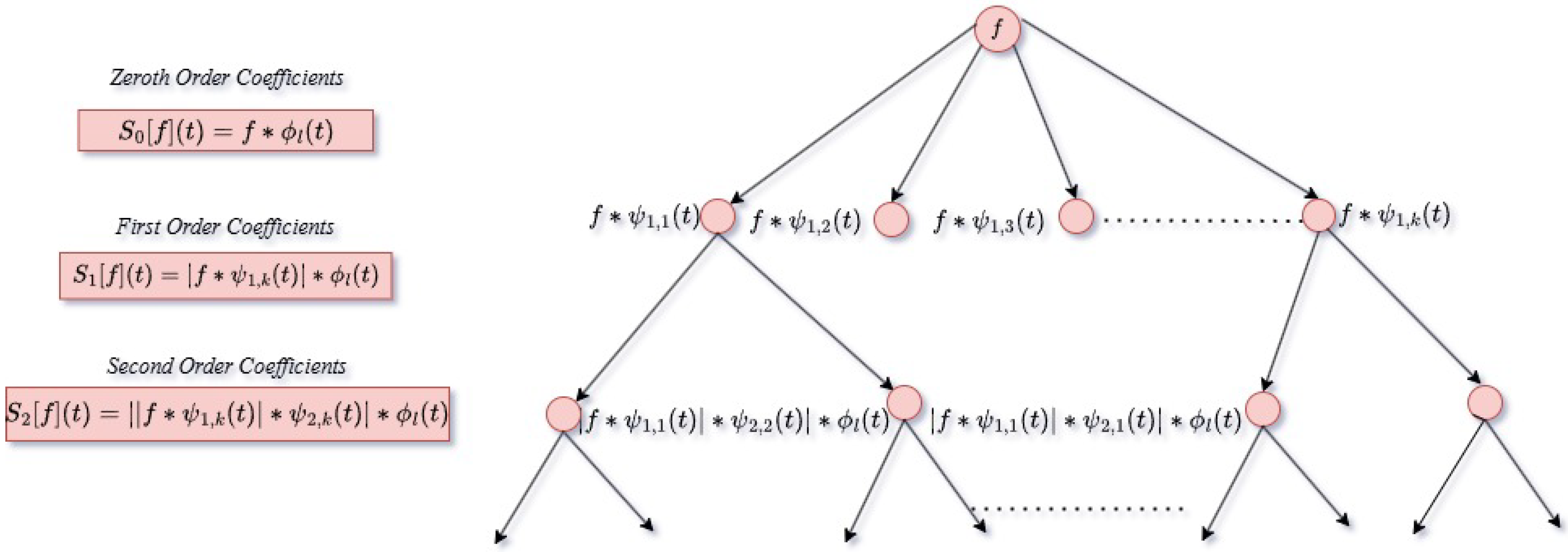
${\psi }_{1,1}\left(t\right),{\psi }_{1,2}\left(t\right),{\psi }_{1,3}\left(t\right),\dots {\psi }_{1,k}\left(t\right)$ and number of wavelet used is k. By taking the modulus of these convolutions, the first-order coefficients are derived. The f is convolved with wavelet functions similar to CWT. The nonlinear modulus operation is applied to these coefficients and convolving the result with the scaling function to obtain the scattering coefficients at level 1:

$$S_1\left[f\right]\left(t\right)=\begin{array}{c}|f\ast {\psi }_{1,1}\left(t\right)|\ast \varphi \left(t\right),|f\ast {\psi }_{1,2}\left(t\right)|\ast {\varphi }_l\left(t\right),\hfill \\ |f\ast {\psi }_{1,3}\left(t\right)|\ast {\varphi }_l\left(t\right),\dots \hfill \\ |f\ast {\psi }_{1,k}\left(t\right)|\ast {\varphi }_l\left(t\right)\hfill \end{array}$$

(9)

$$\begin{array}{cc}\hfill S_{1,1}& =|f\ast {\psi }_{1,1}\left(t\right)|\ast {\varphi }_l\left(t\right),\hfill \\ \hfill S_{1,2}& =|f\ast {\psi }_{1,2}\left(t\right)|\ast {\varphi }_l\left(t\right),\hfill \\ \hfill S_{1,3}& =|f\ast {\psi }_{1,3}\left(t\right)|\ast {\varphi }_l\left(t\right),\dots \hfill \\ \hfill S_{1,k}& =|f\ast {\psi }_{1,k}\left(t\right)|\ast {\varphi }_l\left(t\right)\hfill \end{array}$$

3.

Second-order scattering coefficients:

At level 2, the coefficients in level 1 are further convolved with the wavelet functions at various scales ${\psi }_{2,1}\left(t\right),{\psi }_{2,2}\left(t\right),{\psi }_{2,3}\left(t\right),\dots$ and modulus operation is performed on each.

$$\begin{array}{cc}\hfill S_2\left[f\right]\left(t\right)& =\left\{\begin{array}{c}\left|\right|f\ast {\psi }_{1,1}\left(t\right)|\ast {\psi }_{2,1}\left(t\right)|\ast {\varphi }_l\left(t\right),\hfill \\ \left|\right|f\ast {\psi }_{1,1}\left(t\right)|\ast {\psi }_{2,2}\left(t\right)|\ast {\varphi }_l\left(t\right),\hfill \\ \left|\right|f\ast {\psi }_{1,1}\left(t\right)|\ast {\psi }_{2,3}\left(t\right)|\ast {\varphi }_l\left(t\right),\dots \hfill \end{array}\right.\hfill \\ \hfill & \left\{\begin{array}{c}\left|\right|f\ast {\psi }_{1,2}\left(t\right)|\ast {\psi }_{2,1}\left(t\right)|\ast {\varphi }_l\left(t\right),\hfill \\ \left|\right|f\ast {\psi }_{1,2}\left(t\right)|\ast {\psi }_{2,2}\left(t\right)|\ast {\varphi }_l\left(t\right),\hfill \\ \left|\right|f\ast {\psi }_{1,2}\left(t\right)|\ast {\psi }_{2,3}\left(t\right)|\ast {\varphi }_l\left(t\right),\dots \hfill \end{array}\right.\hfill \end{array}$$

(10)

The scattering network energy is dissipated in each layer. The zeroth-order coefficient averages input signal, so mainly low-frequency information is obtained from this layer [40]. The averaging procedure causes a loss of high-frequency information. The omitted features in the initial step are acquired in the following layers through the use of a CWT, resulting in scalogram coefficients. The coefficients undergo a nonlinear operation and are applied to a low-pass filter to obtain scattering coefficients [41]. Figure 10 shows the layers of the wavelet scattering network. Finally scattering coefficients $S_0\left[f\right]\left(t\right),S_1\left[f\right]\left(t\right),S_2\left[f\right]\left(t\right)$ are concatenated to form a feature matrix

Time invariance: The main property of WST is translation invariance. WST are invariant to translations and stable when the signal undergoes deformation. The duration of the invariance scale is determined by the scaling function.

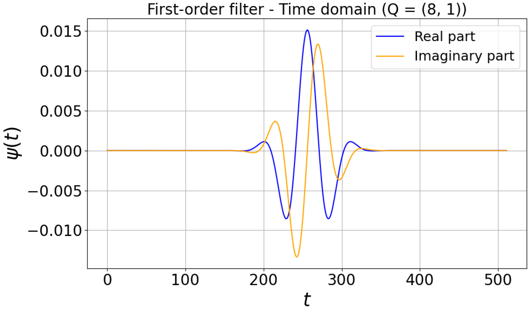
Quality factor and filter banks: The filter banks have a significant role to play in WST and are formed with numerous band-pass filters, where each is designed for a different range of frequencies. Here, the filter banks are constituted by convolving the signal with these wavelets and dividing the signal into various granules of the frequency level for analysis. The quality factor (Q) refers to the number of wavelets per octave in a filter bank. The quality factor determines the frequency resolution of the analysis. Figure 11 portrays the primary band-pass filter of the WST in the time domain using the parameters as $Q=(8,1)$. The most extreme scale of the low-pass filters is dictated by the parameter J which is set as a power of two. The support size T for the filters is selected to be $2^{11}$ given that T must be the power of two, and this magnitude is suitable for the proposed hybrid approach [65]. The plotted wavelet filter is obtained by applying an inverse FFT on the frequency domain of the wavelet [25].

Figure 12 depicts the initial filter bank within the frequency domain. Overall, this depiction demonstrates the multi-scale essence of the WST, displaying how it dissects the signal into constituents that capture different frequency bands, thereby providing a detailed frequency examination.

3.4. Classification

Various classifiers are employed for assessing the performance of the proposed hybrid approach. The subsequent subsections offers indepth descriptions of these classifiers.

3.4.1. Naive Bayes

Naive Bayes classifier applies bayes’ theorem, assuming independence between features. The mathematical statement of bayes theorem:

$$Pr(b\mid a)={\displaystyle \frac{Pr(a\mid b)·Pr\left(b\right)}{Pr\left(a\right)}}$$

(11)

$Pr(b\mid a)$ represents the posterior probability, $Pr(a\mid b)$ denotes the probability of the feature set a given class b, $Pr\left(b\right)$ signifies the prior probability of class b, and $Pr\left(a\right)$ is the evidence.

3.4.2. Support Vector Machine (SVM)

SVM is an ML algorithm where the kernel is a crucial concept in SVM that allows the algorithm to determine the hyperplane that classifies the data. The linear kernel is the simplest form of kernel function. It is defined by the dot product of input vectors. The various kernels used in the SVM model are given below.

Linear kernel:

$$K(x_i,x_j=x_i·x_j$$

(12)

Poly kernel:

$$K(x_i,x_j)={(x_i·x_j+c)}^d$$

(13)

where c is a constant, d is degree of polynomial.

Radial basis function (RBF) kernel:

$$K(x_i,x_j)=exp\left(-\gamma \parallel x_i-x_j{\parallel }^2\right)$$

(14)

where $\gamma$ is a parameter that determines the spread of the RBF kernel.

3.4.3. Random Forest

Random forest is an ensemble decision trees. Random forest is dependent on a set of random variables and multiple learners are built in parallel to improve the results. It applies to both continuous and categorical response variables [23].

3.4.4. Boosting Algorithms

Adaptive boosting (adaBoost) is an ensemble learning algorithm for boosting. It operates by sequentially training models, with each subsequent model concentrating more on instances that were misclassified by its earlier ones. Extreme gradient boosting (XGBoost) is an enhanced gradient boosting learners method that delivers superior ML results and computational performance [66]. The light gradient boosting machine (lightGBM) architecture is based on gradient boosting, employing an ensemble of decision trees to develop a robust predictive model. The emphasis on efficiency is underscored by its leaf-wise tree development approach.

3.4.5. Bagging Algorithms

Bootstrap aggregating is an ensemble learning approach that employs many models and averages their predictions. The bagging classifier is made by majority voting across baselearners [66].

3.4.6. K-Nearest Neighbours (K-NN)

The K-NN is an non-parametric ML technique from the class of supervised methods. K-NN does not create an explicit model against the training data. It categorises new data points on similarity measures.

4. Proposed Methodology

The proposed hybrid framework involves four major steps, namely preprocessing of EEG signals, extraction of dynamic modes from the preprocessed signal, three-layer WST-based feature extraction, and classification using ML models. The block diagram of the proposed hybrid approach is given in Figure 13.

4.1. Preprocessing of EEG Signals

The preprocessing of EEG signals entails of channel selection, filtering, and segmentation. From the multichannel CHB-MIT dataset, 17 EEG channels are selected for all patients [67]. This consistency is important for comparison across the recordings because it minimises variability due to differences in electrode placement or channel configuration. The Bern Barcelona is a two-channel dataset and both channels are used, while the Khas is a single-channel dataset. Two crucial filters are imposed on the EEG signals before any specific analysis. a bandpass filter is employed in the frequency range of 0.5 to 70 Hz. This frequency band covers the majority of the brain activity to be studied and prevents low-frequency drift and high-frequency noises. a 60 Hz notch filter is applied to delete the power line disturbance, which is one of the common noises in the EEG recordings. Both filters are set up in the same manner across these datasets. Further, the filtered signal is segmented into 8 s [68] and passed as input to the DMD module to extract the dynamic modes.

4.2. Extraction of Dynamic Modes

The preprocessed EEG signals are converted into an augmented matrix using Hankelization to effectively capture the inherent dynamics and extract the dynamic modes.

Hankelization

The augmented matrix for the EEG data is computed by the process of Hankelization and is similar to the eigenvalue realization algorithm [63]. To effectively depict the dynamics of brain activity, the number of rows in the augmented matrix needs to be no less than double the number of columns [69]. Data augmentation is performed on the original data matrix X, which represents the EEG recordings with a shape of $N\times L$, where N is the number of channels and L is the number of time points referred as snapshots. An augmented data matrix $X_{\mathrm{aug}}$ is produced by attaching multiple time-shifted versions of the EEG samples by Hankelization. This ensures that the dynamics of brain activities are properly captured [16]. The augmented matrix is represented below.

$$X_{\mathrm{aug}}=\left[\begin{array}{cccc}{x}_1& x_2& \dots & x_{L-k}\\ ⋮& ⋮& \ddots & ⋮\\ x_2& x_3& \dots & x_{L-k+1}\\ ⋮& ⋮& \ddots & ⋮\\ x_k& x_{k+1}& \dots & x_{L-1}\\ ⋮& ⋮& \ddots & ⋮\end{array}\right]$$

(15)

$$X_{\mathrm{aug}}\in {\mathbb{R}}^{(N\times w)\times (L-w+1)}$$

(16)

Here, w is the window size used for augmentation. In the proposed methodology, the number of dynamic modes is fixed based on the reconstruction error. The least reconstruction error is found to be 0.0183 for 200 dynamic modes. Hence, the number of dynamic modes is fixed as 200 in the entire study, which is passed as input to WST for feature extraction.

4.3. WST-Based Feature Extraction

From the literature, it is evident that if the number of orders increases in WST, the energy of the coefficient decreases and approaches to zero. [18] showed that the energy of the third-level (second-order) scattering coefficient can be less than one percent. Motivated by this fact, the proposed methodology involves the extraction of scattering coefficients up to second-order. Energy dissipates more while decomposing through higher levels. applying the WST to dynamic modes yields a characteristic matrix which is the feature matrix. The zeroth-order coefficients are derived by averaging each dynamic mode with the scale function. The size of the resultant matrix is 1 by 213. The first-order coefficients are computed by applying a CWT to each dynamic mode and generating scalogram values. Applying the modulus and filtering to these scalogram coefficients yields a 32 by 213 matrix of first-order coefficients. Similarly, the second-order coefficients form a 17 by 213 matrix by applying the same process to first-order coefficients. These three matrices will form a scattering coefficient matrix of size 50 by 213 for CHB-MIT dataset. Within these matrices, the 213 columns represent the time dimension while the 50 rows reflect the scale dimension after averaging. The scattering coefficient matrix offers a multi-scale and multi-frequency examination of its temporal behaviour. These matrices serve as feature sets for ML and DL applications. The Bern Barcelona dataset is a two-channel dataset with a scattering coefficient matrix of size 50 by 25. The single-channel Khas dataset has a scattering coefficient matrix of size 50 by 13. Figure 14 provides the scattering coefficients of a dynamic mode of different orders. The upper plot depicts the zeroth-order scattering coefficients. The second plot represents the scalogram of the first-order scattering coefficients. The last plot is the scalogram of second-order coefficients which identifies the interactions and more complex structures within the mode [70]. The proposed DMD-WST algorithm on the EEG signal is represented in Algorithm 1.

Algorithm 1 Proposed hybrid DMD-WST algorithm

Input: Data matrix $X_{\mathrm{aug}}$, wavelet function $\psi \left(t\right)$, scaling function ${\varphi }_l\left(t\right)$ Output: DMD modes $\Phi$ and wavelet scattering coefficients $S_0,S_1,S_2$ Step 1: Compute SVD of the data matrix, substitute $X_{\mathrm{aug}}$ into $X_{\mathrm{aug}}^{\prime }$: Compute $X_{\mathrm{aug}}=US{V}^{*}$ Step 2: Compute the matrix $\tilde{A}$ Compute $\tilde{A}=U^{*}{X}_{\mathrm{aug}}^{\prime }V{S}^{-1}$ Step 3: Calculate eigenvalues and eigenvectors of $\tilde{A}$ Solve $\tilde{A}W=W\Lambda$ Step 4: Compute DMD modes $\Phi$ corresponding to the DMD eigenvalues Compute $\Phi =X_{\mathrm{aug}}^{\prime }V{S}^{-1}W$ where f is the each DMD mode Step 5: Compute WST Compute Zeroth-order coefficient $S_0\left[f\right]\left(t\right)=|f\ast {\varphi }_l\left(t\right)|$ for k = 1, 2, …, K do     Compute first-order coefficients:     $S_1\left[f\right]\left(t\right)=|f\ast {\psi }_{1,k}\left(t\right)|\ast {\varphi }_l\left(t\right)$ end for for k = 1, 2, …, K do    for j = 1, 2, …,J do        Compute second-order coefficients:        $S_2\left[f\right]\left(t\right)=\left|\right|f\ast {\psi }_{1,k}\left(t\right)|\ast {\psi }_{2,j}\left(t\right)|\ast {\varphi }_l\left(t\right)$     end for end for Step 6: Wavelet scattering coefficients $S_0\left[f\right]\left(t\right)$, $S_1\left[f\right]\left(t\right)$, $S_2\left[f\right]\left(t\right)$ which is a scattering matrix is given as an input to the ML

4.4. Classification Using ML Model

The proposed approach utilised traditional ML approaches for classification. The generated scattering coefficients are used as features for classification. Ensemble approaches, including random forest, bagging, XGBoost, adaBoost, and lightGBM, are utilised in this study. The K-NN and Naive Bayes classifiers offer further comparative insights into the proposed methodology. Furthermore, SVM with kernels such as linear, RBF, and poly are employed to assess their efficacy.

5. Experimental Results

The experiments were executed on a system featuring an AMD Ryzen 7 4800H processor (Advanced Micro Devices, Inc., Santa Clara, CA, USA) with radeon graphics, functioning at 2.90 GHz, and 16.0 GB of RAM. The python libraries used for the implementation include pydmd for DMD and kymatio for WST. The scattering transform is determined by the parameters such as quality factor (Q), low-pass filter scale (J), and support size (T). These are the fundamental parameters of choice that specify the filters to be used. In the case of small J value, scattering energy is concentrated in the low-order terms (more than 95%), thus the high-order coefficients play an insignificant role in signal representation. Increasing J transfers energy and captures richer temporal characteristics, but very large scales become redundant, causing energy leakage and excessive growth of coefficients that greatly increases the computational complexity. To trade off these considerations, we tested J = 3 and J = 4 offered better representation than J = 2. The J = 4 produced consistently better classification accuracy. It is with this consideration that J = 4 is selected as the best tradeoff between accuracy, efficiency and interpretability. Based on the available literature, $J=4$ and $Q=8$ is a suitable choice for the proposed method [40,41,65]. The experiments for the proposed hybrid approach are conducted using the datasets discussed in Section 3. The CHBMIT dataset is categorized into seizure and nonseizure. The two-channel Bern Barcelona dataset includes two classes, namely focal and non-focal. The Khas dataset consists of three data classes namely inter-ictal, ictal, and preictal. From the CHB-MIT dataset, 106 seizure segments have been selected, followed by an equal number of non-seizure segments to maintain class balance. In the Barcelona dataset, 100 records are used for both focal and non-focal classes. The KHaS dataset has 50 records for each of the preictal, ictal, and interictal stages. Each segment is decomposed into 200 dynamic modes using DMD. WST coefficients are derived from each dynamic mode and used as input features for classification. The scattering matrix generated for each dynamic mode has a dimension of 50 × 213 for the CHB-MIT dataset, 50 × 25 for the Barcelona dataset, and 50 × 13 for the Khas dataset. The dynamic modes within the same EEG recording are assigned entirely to either the training set or the testing set to prevent data leakage. Each dynamic mode is individually classified, and a majority voting scheme is applied across the modes of each segment to classify the recording as seizure or non-seizure. Data is allocated into a training set with 80% and a testing set with 20%. The method is accessed using 10-fold cross-validation. The details of the hyperparameters for various classifiers used in the hybrid approach are provided in

Table 2. Hyperparameter for various classifiers using grid-search CV.

Classifiers	Parameter
Random forest	n_estimators = 100, random_state = 42
XGBoost	n_estimators = 500, learning_rate=1.0, max_depth = 3, random_state=42
adaBoost	n_estimators = 100, learning_rate = 0.1, random_state = 42
bagging	n_estimators = 100, random_state = 42
SVM (linear)	C_value = 100, random_state = 42
SVM (RBF)	C_value = 100, gamma_value = 0.01
SVM (Poly)	C_value = 100, gamma_value = 0.01, degree_value = 3, coef_value = 1
LightGBM	n_estimators = 100, learning_rate = 0.1, random_state = 42

. For an 8-s window with 200 modes, the total inference time per segment was 0.724 s, corresponding to an average inference time of 0.1037 ms per sample, which remains well within the practical real-time range.

5.1. Evaluation Metrics

The proposed methodology is assessed using accuracy, F1 score, precision, G-mean, Cohen’s kappa, sensitivity, and Matthews correlation coefficient. The value of $TP$ shows that the prediction is true and positive, $FP$ represents an incorrectly predicted positive outcome, $FN$ counts the model mistook a positive response as negative, and $TN$ is the correctly predicted negative outcome [71].

5.1.1. Precision

It is the ratio of correct positive outcomes to the total predicted positive outcomes.

$$\mathrm{Precision}={\displaystyle \frac{TP}{TP+FP}}$$

(17)

5.1.2. Sensitivity

The true positive predictions are divided by the total number of actual positive instances. Recall is another term in the context of binary classification, both of which are referred to using the same equation.

$$\mathrm{Sensitivity}={\displaystyle \frac{TP}{TP+FN}}$$

(18)

5.1.3. F1 Score

F1 score is calculated as the harmonic mean of precision and sensitivity.

$$F1=2·{\displaystyle \frac{\mathrm{precision}·\mathrm{sensitivity}}{\mathrm{precision}+\mathrm{sensitivity}}}$$

(19)

5.1.4. Accuracy

It is calculated as the ratio of true positives and true negatives and the total number of predictions [67].

$$\mathrm{Accuracy}={\displaystyle \frac{TP+TN}{TP+TN+FP+FN}}$$

(20)

5.1.5. Cohen’s Kappa

The kappa coefficient which is generally known as Cohen’s kappa ($\kappa$) measures the level of agreement between two classifiers in every class. It adjusts for chance agreement, allowing a better evaluation of agreement than simple accuracy.

$$\begin{array}{cc}\hfill \kappa & ={\displaystyle \frac{2·(TP·TN-FP·FN)}{(TP+FP)·(FP+TN)+(TP+FN)·(FN+TN)}}\hfill \end{array}$$

(21)

5.1.6. Matthews Correlation Coefficient (MCC)

The MCC is a variant of Cramer’s rule [72] applied to a traditional $2\times 2$ confusion matrix [73]. The metric is defined as:

$$\mathrm{MCC}={\displaystyle \frac{TP·TN-FP·FN}{\sqrt{(TP+FP)(TP+FN)(TN+FP)(TN+FN)}}}$$

(22)

5.1.7. G-Mean

A classifier’s geometric mean (G-mean) is determined by square root of the product of specificity and sensitivity.

5.1.8. Confusion Matrix

Confusion matrix is a table layout that represents how many times the model has predicted correctly and incorrectly.

$$\left[\begin{array}{cc}TP\left(\mathrm{true}\mathrm{positives}\right)& FP\left(\mathrm{false}\mathrm{positives}\right)\\ FN\left(\mathrm{false}\mathrm{negatives}\right)& TN\left(\mathrm{true}\mathrm{negatives}\right)\end{array}\right]$$

5.2. Performance Analysis

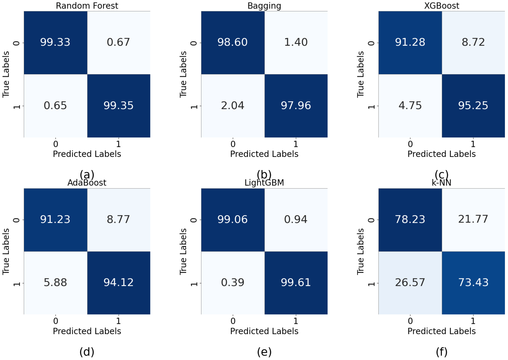
This section reports the outcomes of experiments evaluating various classifiers. In the CHB-MIT dataset, the channels utilised are: FP1-F7, F8-T8, FZ-CZ, FP2-F8, P3-O1, C3-P3, F7-T7, C4-P4, F4-C4, P8-O2, CZ-PZ, P7-O1, P4-O2, FP1-F3, F3-C3, FP2-F4, and T7-P7. Augmentation was performed based on Hankelization to acquire the full dynamics of the EEG. Initially, the augmented EEG segments are processed using DMD and then WST is applied to capture the features. The computed features are organized into a matrix, which is subsequently used to classify them into seizures and nonseizures.

Table 3. Performance evaluation for different algorithms on CHB-MIT dataset using proposed method.

Algorithm	Precision	Sensitivity	F1 Score	Accuracy (%)
Random forest	0.99	0.99	0.99	99
XGBoost	0.93	0.93	0.93	93
AdaBoost	0.93	0.93	0.93	93
Bagging	0.99	0.99	0.99	98.8
SVM (linear)	0.67	0.68	0.68	68
SVM (RBF)	0.88	0.91	0.89	89
SVM (Poly)	0.95	0.95	0.95	94.61
LightGBM	0.99	0.99	0.99	99
K-NN	0.76	0.76	0.76	77
Naive Bayes	0.80	0.79	0.79	80

shows the comparison using accuracy, precision, sensitivity, and F1 score over nonseizure (class 0) and seizure (class 1) using 10-fold cross-validation. The accuracy, sensitivity, precision, and F1 Score is a multi-perspective performance evaluator for ML. Random forest and bagging provide better precision, sensitivity, and F1 scores for both classes compared to other classifiers. The results in

Table 4. Cohen’s kappa and MCC value for different algorithms on CHB-MIT using proposed method.

Algorithm	Cohen’s Kappa	MCC	G-Mean
Random forest	0.98	0.98	0.99
XGBoost	0.86	0.87	0.93
AdaBoost	0.85	0.85	0.925
Bagging	0.98	0.98	0.99
LightGBM	0.99	0.99	0.99
SVM (RBF)	0.77	0.79	0.89
SVM(Poly)	0.89	0.89	0.95

present the kappa and MCC values for various classifiers. Random forest performs well by achieving the best accuracy of 99% and with Cohen’s kappa and MCC both reaching 0.98. The values of sensitivity, F1 score, and precision obtained from the random forest are 0.99, 0.99, and 0.99, respectively. The bagging method provides 98.8% for accuracy. It attained values of MCC and Cohen’s kappa of 0.98. LightGBM shows a high MCC and Cohen’s kappa of 0.99. This suggests that these models perform well in detecting seizures and nonseizures. Hence the proposed hybrid method would be a promising approach for classifying seizure segments. From Table 3 the results indicate that adaBoost achieved an accuracy of 93%. Cohen’s kappa and the MCC both reached a value of 0.85. XGBoost reports an accuracy of 93%, Cohen’s kappa of 0.86, and MCC of 0.87 which is slightly higher than adaBoost. Both with low levels of false positives and relatively high sensitivity values. LightGBM demonstrates commendable performance in comparison to other boosting techniques. In particular, its precision and sensitivity scores are 99%, which is almost the same as that of random forest. The G-mean values provide the information related to the balance between the sensitivity and specificity of each classifier. The highest G-mean is recorded with random forest, lightGBM and bagging of 0.99. XGBoost and adaBoost attained G-mean values of 0.93 and 0.925, respectively. In Table 3, the performance of SVM with linear, RBF, and polynomial kernels is also assessed based on evaluation metrics. It is observed that the linear kernel shows an accuracy of 68%. The RBF kernel and poly have higher performance metrics than linear SVM. The RBF kernel improves performance by achieving a sensitivity of 91%. The SVM poly kernel outperforms both XGBoost and adaBoost with an accuracy of 94.61%, which is higher than the accuracy of 93% achieved by both boosting models. This suggests that the poly kernel is particularly effective at capturing the non-linear relationships in the data. The overall results of the CHBMIT dataset are mentioned in Figure 15. Figure 16 shows the confusion matrix of different classifiers on CHB-MIT dataset. The confusion matrix of the random forest presents a very low number of misclassifications, which consists of only 26 false positives and 25 true negatives. The confusion matrix shows that random forest performs very well in classification problems with just a small upper hand over bagging and lightGBM on all performance metrics. Contrarily, the confusion matrices of XGBoost and adaBoost are very similar to each other with a bit more misclassification in comparison to random forest. K-NN classifier obtained a mean accuracy of around 75.83% on 10-fold cross-validation.

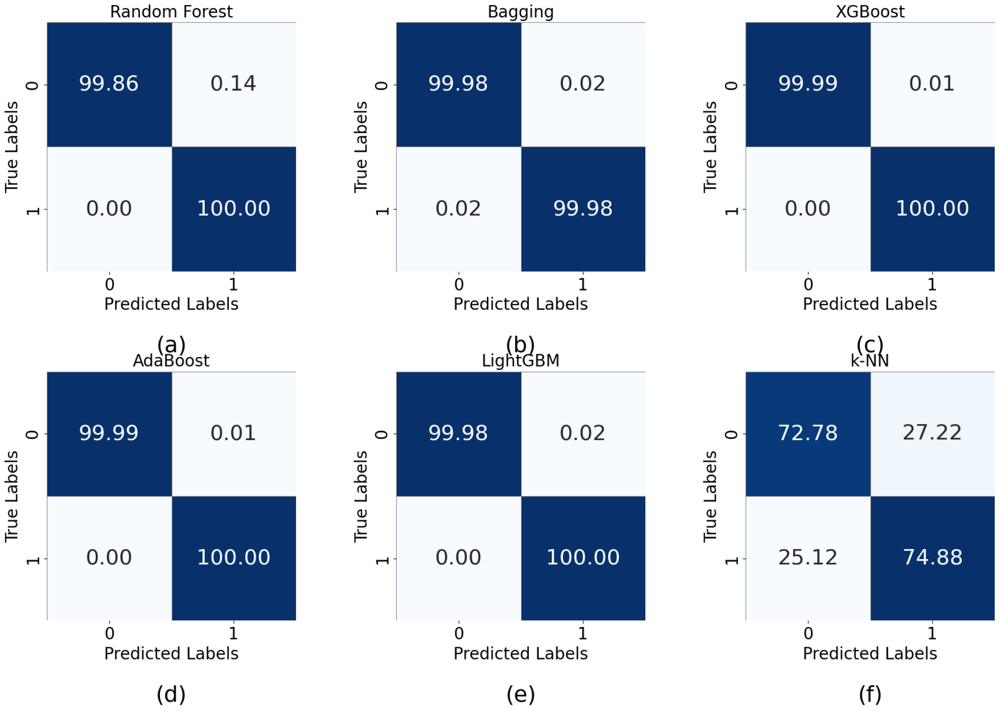
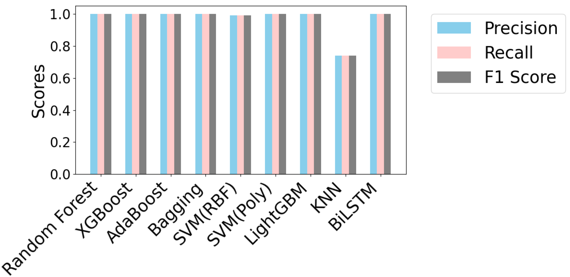
The focal and non-focal EEG classification is considered in the Bern Barcelona dataset and

Table 5. Performance evaluation for different algorithms on Bern Barcelona dataset using proposed method.

Algorithm	Precision	Sensitivity	F1 Score	Accuracy (%)
Random forest	1.00	1.00	1.00	100
XGBoost	1.00	1.00	1.00	100
AdaBoost	1.00	1.00	1.00	100
Bagging	1.00	1.00	1.00	100
SVM (linear)	0.65	0.65	0.65	65
SVM (RBF)	0.99	0.99	0.99	98
SVM (Poly)	1.00	1.00	1.00	100
LightGBM	1.00	1.00	1.00	100
K-NN	0.74	0.74	0.74	77
Naive Bayes	0.49	0.49	0.50	50

highlights the classification metrics of different classifiers on the Bern Barcelona dataset. The confusion matrices of different algorithms are displayed in Figure 17. Almost all the models such as random forest, XGBoost, adaBoost, bagging, and lightGBM give 100% on evaluation metrics like accuracy, precision, sensitivity and F1 score. The K-NN has poor metrics for precision, sensitivity, F1 score and accuracy. In particular, K-NN struggles more than the other methods is probably because this method can be sensitive to the choice of distance metric and number of neighbours. Since its performance depends on data distribution, it is not always the best solution. The MCC, kappa and G-mean values for different classifiers on Bern Barcelona are listed in

Table 6. Cohen’s kappa and MCC metrics for the proposed method across different algorithms on Bern Barcelona dataset.

Algorithm	Cohen’s Kappa	MCC	G-Mean
Random forest	1.00	1.00	1.00
XGBoost	1.00	1.00	1.00
AdaBoost	1.00	1.00	1.00
Bagging	1.00	1.00	1.00
LightGBM	1.00	1.00	1.00
SVM (RBF)	0.98	0.98	0.99
SVM (Poly)	1.00	1.00	1.00

. The overall performance metrics using multiple classifiers on the Barcelona dataset are shown in Figure 18.

Furthermore, the proposed hybrid approach is tested using the Khas dataset. The proposed methodology classified segments into inter-ictal, ictal and preictal. The

Table 7. Performance evaluation for different algorithms on Khas dataset using proposed method.

Algorithm	Precision	Sensitivity	F1 Score	Accuracy (%)
Random forest	1.00	1.00	1.00	100
XGBoost	1.00	1.00	1.00	100
AdaBoost	1.00	1.00	1.00	100
Bagging	1.00	1.00	1.00	100
SVM (linear)	0.62	0.62	0.62	62
SVM (RBF)	0.97	0.97	0.97	96.87
SVM (Poly)	0.99	0.99	0.99	99
LightGBM	0.99	0.99	0.99	99
K-NN	0.57	0.58	0.58	58
Naive Bayes	0.57	0.57	0.57	57

compared the performance among various classifiers and obtained high accuracy for most of the classifiers. The highest accuracy of 100% is recorded with the boosting algorithms, bagging and random forest. The confusion matrix of all six classifiers on the Khas dataset is given in Figure 19. The lowest accuracy was reported in K-NN and Naive Bayes. The SVM RBF and poly kernel showed an accuracy of 97% and 99%, respectively. Considering the overfitting influence 10-fold cross-validation is conducted on the three datasets. The result obtained from the best-performed classifiers for 10-fold cross-validation of three datasets is shown in Figure 20. According to the 10-fold cross-validation plot across all datasets, it is observed that the proposed approach performs well and provides better accuracy. according to the result, it is evident that DMD effectively captures variations in duration and amplitude of nonlinear information, which are crucial for understanding brain dynamics. Consequently, the WST is employed to generate a more detailed representation of modes, facilitating the detection of subtle changes associated with seizure. Furthermore, when integrated with DMD, WST features effectively enhance the analysis and detection of seizure patterns. DMD’s ability to identify coherent dynamic structures helps reduce redundancy in high-dimensional EEG data while preserving essential discriminative features. This procedure enhances the distinct differentiation between seizure and non-seizure states, leading to improved accuracy and interpretability in seizure classification.

6. Discussion

The hybrid method focuses on the classification of seizures relying on DMD and a three-layer wavelet scattering network. The ML algorithms including SVM, K-NN, Naive Bayes, random forest, adaBoost, XGBoost, and lightGBM are evaluated for the seizures and nonseizure segments classification. The findings suggest that the ensemble-based classifiers, poly and RBF SVM show better performance in both classification accuracy and generalization ability than traditional classifiers such as K-NN, and Naive Bayes. Additionally, the use of cross-validation confirms reliability across different datasets.

The receiver operating characteristic (ROC) curves of the hybrid approach are shown in Figure 21. The random forest, bagging classifier, and lightGBM classifiers perform perfectly with an area under the curve (AUC) of 1.0. Excellent performances are also seen in the XGBoost and adaBoost algorithms, scoring an AUC of 0.99. The kNN classifier has an AUC of 0.75, indicating that its classification performance is weaker compared to the other classifiers.

Table 8. Comparison of proposed methodology with related articles for epilepsy classification on CHB-MIT dataset.

Author	Feature Extraction	Classification	Performance
Bhattacharya and Pachori et al. (2017) [13].	Empirical WT	Random forest, linear Naive bayesK-NN classifiers	Accuracy 0.99 Sensitivity 0.97
Li et al. (2021) [59]	Common spatial pattern wavelet transform and EMD	SVM	Sensitivity 0.97
Shen et al. (2022) [14]	DB16-DWT	RUSBoosted tree ensemble models	Accuracy 0.96,Sensitivity 0.96
Zarei et al. (2021) [46]	DWT, orthogonal matching pursuit, statistical features, entropy features	SVM	Accuracy 0.97Sensitivity 0.97
Jiang et al. (2021) [76]	Synchroextracting chirplet transform	SVM	Accuracy 0.99 MCC 0.97
Alharati et al. (2021) [4]	DWT	CNN	Accuracy 0.96 Sensitivity 0.96
Tian et al. (2021) [77]	FFT and WPD	CNN	Accuracy 0.98 Sensitivity 0.96
Bilal et al. (2019) [39]	MRDMD and temporal features	RUSBoost	Sensitivity 0.937
Zhang, Jincan and Zheng et al. (2024) [74]	DWT and time–frequency domain and nonlinear features	CNN-gated recurrent unit-attention mechanism	Accuracy 0.99 Sensitivity 0.99
Kumar Priyaranjan et al. (2025) [75]	Mean, skewness, kurtosis, and STFT	EpiCNN-LSTM	Accuracy 0.99 Sensitivity 0.99
Solaija et al. (2018) [16]	DMD, DMD power and curve-length	RUSBoost	Sensitivity 0.87
Xiang et al. (2015) [78]	Fuzzy entropy and sample entropy	SVM	Accuracy 0.98 Sensitivity 0.98
Cura and akan et al. (2021) [17]	Higherorder, DMD spectral moments, DMD sub-band power.	Random forest	Accuracy 0.96 Sensitivity 0.92
Zeynab et al. (2025) [44]	Weighted visibility graph (WVG) features	Random forest	Accuracy 0.94 Sensitivity 0.92
Proposed method	DMD-WST	Random forest	Accuracy 0.99 Sensitivity 0.99 MCC 0.98

shows that seizure classification with the CHB-MIT dataset achieved enhanced accuracy and sensitivity values compared to previous studies. Ref. [17] implemented seizure detection using the CHB-MIT dataset with the DMD method, and obtained an accuracy of 96% with DMD power and moment-based features. Similarly, ref. [16] also applied the DMD method in a personalized manner and reported a sensitivity of 0.87%. The WST is comparable in architecture to CNN. CNN works in layers consisting of convolutions, nonlinearity, and pooling. WST works pretty well with few data which is very important for seizure classification. Ref. [4] obtained an accuracy of 0.96 using CNN. The table illustrates that the proposed method outperforms traditional machine learning approaches employing various feature extraction techniques. Moreover, it attains performance levels similar to those of leading deep learning models. Most of the deep learning approaches achieve high accuracy and sensitivity, they depend on manually extracted features such as DWT, STFT, mean, and skewness. These models often utilise architectures, such as CNNs combined with GRUs, LSTMs, and attention mechanisms, further increasing computational demands [74,75]. We performed experiments based on VMD and WST as feature extraction methods and used various classifiers. The findings demonstrated that lightGBM had the highest accuracy of 97.86% with a sensitivity and F1-score of 0.97, and as well, random forest scored 97.25% accuracy and a sensitivity and F1-score of 0.96. Conversely, adaBoost is only able to achieve an 85% accuracy, sensitivity, and F1-score. However, these scores remain slightly less than the ones that were achieved through the proposed hybrid approach (DMD + WST), which has an accuracy rate of 99%, which illustrates the strength of using DMD together with WST in representing features more strongly. Conversely, AdaBoost achieves much lower accuracy compared to our proposed hybrid approach.

Table 9. Comparison of proposed methodology with related articles for epilepsy classification on Bern Barcelona dataset.

Author	Feature Extraction	Classification	Performance
Sadiq et al. (2021) [79]	Tunable Q-factor wavelet transform (TQWT) entropy features	Cascade-forward neural network	Accuracy 0.97 Sensitivity 0.97
Kumar and Rao et al. (2019) [80]	VMD differential entropy	Random forest	Accuracy 0.78
San-Srgundo et al. (2019) [81]	EMD	DNN	Accuracy 0.989
al salmon et al. (2022) [82]	Dual-tree complex WT and fast fourier transform	Least squareSVM	Accuracy 0.968
Supriya et al. (2021) [83]	Edge weight fluctuation (EWF)	SVM	Accuracy 0.99 Sensitivity 1.00
Wang et al. (2021) [84]	Multi-branch DL fusion model	CNN	Accuracy 0.97 Sensitivity 0.97
akbari and Sadiq et al. (2021) [85]	Kruskal–Wallis statistical test	SVM	accuracy 0.93 Sensitivity 0.96
anuragi et al. (2023) [86]	Fourier–Bessel series expansion-based EWT	Least squareSVM	Accuracy 0.98
Srinath and Gayathri et al. (2023) [87]	EMD	CNN FCM	Accuracy 0.99
Fasil and Rajesh et al. (2019) [88]	Exponential energy features	SVM	Accuracy 0.89
Proposed method	DMD-WST	Random forest	Accuracy 1.00 Sensitivity 1.00MCC 1.00

conducts a comparative analysis of different methodologies for epilepsy classification based on the Bern Barcelona dataset. Each study employs distinct feature extraction techniques and classification methods yielding different performance outcomes. From the table, the proposed method showed high accuracy across all classifiers utilizing the Bern Barcelona dataset.

The multi-class classification is performed using Khas dataset. Benchmarking against other advanced approaches with the Khas dataset is given in

Table 10. Comparison of proposed methodology with related articles for epilepsy classification on Khas dataset.

Author	Feature Extraction	Classification	Performance
Chakraborty et al. (2021) [89]	Multiscale spectralfeatures	Random forest	Accuracy 0.989 sensitivity 0.981
Du et al. (2022) [5]	Optimized feature CNN model for feature extraction	SVM	Accuracy 0.98 Sensitivity 1.00
Shanmughan et al. (2024) [90]	DWT	Non-Linear SVM	Accuracy 0.88 Sensitivity 1.00
Buldu et al. (2024) [91]	CWT	CNN	accuracy 0.95Sensitivity 0.96
Proposed method	DMD-WST	Random forest	Accuracy 1.00Sensitivity 1.00

. The proposed methodology provides better performance compared to the other related articles. Many existing methods in the Khas dataset have used binary classification (ictal-preictal, preictal-inter-ictal, inter-ictal-ictal), whereas our proposed method employs multiclass classification, achieving better performance. The classification methodology offers a range of remarkable advantages in terms of clinical significance and generalisability. The model would acquire robust patterns related to seizures as a result of training and testing on the data of various individuals, regardless of the variation among patients. The model acquires consistent seizure-related patterns by training and testing on different recordings from all patients, regardless of intra-patient variability. This reduces the risk of overfitting to patient-specific artifacts and provides a more realistic assessment of performance across unseen recordings.

6.1. Confidence Score and Confidence Intervals

The confidence score is a way to calculate the probability of how certain a ML model is about a given prediction. It ranges between 0 and 1. It informs users about the degree of “trust” one should put when using the predictions. The higher the score, the more confident that its prediction will be correct. The lower the confidence score, the less certain of its predictions. Confidence scores reflect the correctness and provide another layer of transparency on the model predictions [71,92].

The Figure 22 shows the histograms of predicted confidence scores from a model across the datasets, where the majority of confidence scores are concentrated close to 1.0. The x-axis represents the range of confidence scores, while the y-axis is the count of predictions at that score level. The confidence threshold of 0.8, for “high confidence” predictions is highlighted in the figure. The CHB-MIT shows a wider spread of confidence scores, with a significant number of predictions distributed between 0.5 and 1.0. across the Bern Barcelona and Khas datasets, almost all of the predictions are above 0.8, and most at around 1.0. It shows that for these datasets, the confidence of predictions made by the model is extremely high. For the CHB-MIT dataset, the confidence interval is [0.9930, 0.9974]. The confidence interval of Barcelona dataset is [1.0000, 1.0000] and the confidence interval for the Khas dataset is [0.9990, 1.0000]. These results report that the model is always able to make the correct prediction for all samples across all datasets.

6.2. Statistical Hypothesis Tests

The effectiveness of the hybrid method is confirmed with multiple statistical hypothesis tests. The hypothesis testing composed of a null hypothesis $\left(H_0\right)$ and an alternative hypothesis $\left(H_1\right)$ to compare the classifiers. The alternative hypothesis ($H_1$) states that the classifier differs. The Friedman test is a non-parametric method for deciding whether the classifier’s performance is significantly different [93]. In the Friedman test the effect size quantifies the magnitude of observed differences and is measured using Kendall’s W values that range from 0 (no differences) to 1 (perfect agreement). A post hoc test is used after a statistical test (like the Friedman test) to indicate the overall difference. If significant difference is found, $H_0$ is rejected after performing the Friedman test. Subsequently, the post hoc Nemenyi test is established to determine the significant differences among the algorithms. The Nemenyi compares all possible pairs of algorithms and produces p values [71,94]. The

Table 11. Friedman test results for different datasets.

Dataset	Friedman Test Statistic	p Value	Kendall’s W [95% CI]
CHB-MIT	15.846	0.00036	0.208 [0.202, 0.2451]
Bern Barcelona	6.500	0.0387	0.026 [0.002, 0.0868]
Khas dataset	15.250	0.00048	0.164 [0.116, 0.208]

shows the Friedman test statistics and corresponding p values for all three datasets. Since the p value is below 0.05 for all three datasets, $H_0$ is rejected.

Table 12. Nemenyi post-hoc test results for different datasets with corrected p-values and Cliff’s $\delta$.

Dataset	Comparison	Corrected p-Value	Cliff’s $\mathit{\delta }$ [95% CI]	Significance
CHB-MIT	Random Forest vs Bagging	0.78047	$-0.12$ [−0.62, 0.38]	NSF
	Random Forest vs LightGBM	0.00716	1.00 [1.0, 1.0]	SDF
	Bagging vs LightGBM	0.00066	1.00 [1.0, 1.0]	SDF
Bern Barcelona	Random Forest vs LightGBM	0.37206	−0.40 [−0.7, −0.1]	NSF
	Random Forest vs XGBoost	0.57290	−0.30 [−0.7, 0.1]	NSF
	LightGBM vs XGBoost	0.93987	0.10 [0.0, 0.3]	NSF
Khas	Random Forest vs AdaBoost	0.00497	1.00 [1.0, 1.0]	SDF
	Random Forest vs XGBoost	0.97281	−0.02 [−0.52, 0.44]	NSF
	AdaBoost vs XGBoost	0.01021	−0.95 [−1.0, −0.8]	SDF

Note: NSF- No significant difference, SDF- Significant difference.

shows p values of the Nemenyi test for different datasets. The table displays the performance of the Nemenyi test. The significant difference (SDF) in performance is indicated by a p value below 0.05, while no significant difference (NSF)in performance is shown by a p value above 0.05. The corrected p value indicates the statistical significance difference of the performance between two models. Cliff’s $\delta$ quantifies the magnitude and direction of such difference with its 95% confidence interval indicating the likely range of the true effect. The statistics show that in most cases, there are no significant changes in classifier performance, which emphasizes that the features enhance efficacy across various ML classifiers. The Friedman test indicates statistically significant differences among models for the CHB-MIT and Khas datasets, while the Bern Barcelona dataset shows only marginal differences. Kendall’s W values are low to moderate, which suggests that although overall rankings differ, there is limited agreement among models’ performances. Nemenyi tests indicate lightGBM has larger effect sizes than random forest and bagging, whereas random forest and bagging do not show significant change for the CHB-MIT dataset. The pairwise comparisons are non-significant and effect sizes are small, indicating that the no significant difference in Bern Barcelona. In the Khas dataset, adaboost shows a significant difference with very large effect sizes, whereas random forest and xgboost perform similarly with no significant difference. Overall, these results indicate that model performance differences are dataset-dependent, with some datasets exhibiting superiority over specific models and others showing no significant difference in performance. The findings of the statistical hypothesis test suggest that the model improves the efficiency of classification.

7. Conclusions

The proposed framework for epileptic signal classification by integrating DMD and WST examines the feasibility of developing a seizure classification approach. The filtered and segmented EEG signals are decomposed into modes corresponding to distinct spatiotemporal patterns using the DMD algorithm. Then, WST is applied to modes to extract the scalogram coefficients, which represent the feature matrix. Performance is evaluated using different ML classifiers, including random forest, SVM, K-NN, bagging, and boosting. This approach works well in capturing dynamic patterns using DMD and extracting multi-scale, translational-invariant features using WST. The proposed method aims to contribute to the advancement of more accurate and efficient tools for seizure classification. The hybrid approach is validated using three publicly available datasets. Random forest and boosting techniques yield 99% and 93% of accuracy, respectively, on the CHB-MIT dataset, whereas Bern Barcelona and Khas datasets yield 100% of accuracy. These findings exhibit valuable insights for classifying seizures. The results from the proposed hybrid methodology are assessed alongside the different existing approaches, and performance is found to be satisfactory.

References

1. World Health Organization (WHO), Global Campaign Against Epilepsy. Atlas: Epilepsy Care in the World; World Health Organization (WHO) Department of Mental Health and Substance Abuse, International Bureau for Epilepsy: Geneva, Switzerland, 2005. [Google Scholar]
2. Brodie, M.J.; Zuberi, S.M.; Scheffer, I.E.; Fisher, R.S. The 2017 ILAE classification of seizure types and the epilepsies: What do people with epilepsy and their caregivers need to know? Epileptic Disord. 2018, 20, 77–87. [Google Scholar] [CrossRef]
3. Wang, L.; Xue, W.; Li, Y.; Luo, M.; Huang, J.; Cui, W.; Huang, C. Automatic epileptic seizure detection in EEG signals using multi-domain feature extraction and nonlinear analysis. Entropy 2017, 19, 222. [Google Scholar] [CrossRef]
4. Alharthi, M.K.; Moria, K.M.; Alghazzawi, D.M.; Tayeb, H.O. Epileptic Disorder Detection of Seizures Using EEG Signals. Sensors 2022, 22, 6592. [Google Scholar] [CrossRef] [PubMed]
5. Du, R.; Huang, J.; Zhu, S. EEG-Based Epileptic Seizure Detection Model Using CNN Feature Optimization. In Proceedings of the 2022 15th International Congress on Image and Signal Processing, BioMedical Engineering and Informatics (CISP-BMEI), Beijing, China, 5–7 November 2022; pp. 1–6. [Google Scholar] [CrossRef]
6. Andrzejak, R.G.; Schindler, K.; Rummel, C. Nonrandomness, nonlinear dependence, and nonstationarity of electroencephalographic recordings from epilepsy patients. Phys. Rev. E—Stat. Nonlinear Soft Matter Phys. 2012, 86, 046206. [Google Scholar] [CrossRef]
7. Swami, P.; Panigrahi, B.; Nara, S.; Bhatia, M.; Gandhi, T. EEG Epilepsy Datasets. 2016. Available online: https://www.researchgate.net/publication/308719109_EEG_Epilepsy_Datasets (accessed on 24 September 2025).
8. Hussain, S.J. Epileptic Seizure Detection Using Wavelets and EMD. In Proceedings of the 2018 Fourth International Conference on Biosignals, Images and Instrumentation (ICBSII), Chennai, India, 22–24 March 2018; pp. 206–212. [Google Scholar]
9. Quintero-Rincón, A.; Pereyra, M.; d’Giano, C.; Risk, M.; Batatia, H. Fast Statistical Model-Based Classification of Epileptic EEG Signals. Biocybern. Biomed. Eng. 2018, 38, 877–889. [Google Scholar] [CrossRef]
10. Li, M.; Sun, X.; Chen, W. Patient-Specific Seizure Detection Method Using Nonlinear ModeDecomposition for Long-Term EEG Signals. Med. Biol. Eng. Comput. 2020, 58, 3075–3088. [Google Scholar] [CrossRef]
11. Aayesha; Qureshi, M.B.; Afzaal, M.; Qureshi, M.S.; Fayaz, M. Machine learning-based EEG signals classification model for epileptic seizure detection. Multimed. Tools Appl. 2021, 80, 17849–17877. [Google Scholar] [CrossRef]
12. Varlı, M.; Yılmaz, H. Multiple classification of EEG signals and epileptic seizure diagnosis with combined deep learning. J. Comput. Sci. 2023, 67, 101943. [Google Scholar] [CrossRef]
13. Bhattacharyya, A.; Pachori, R.B. A Multivariate Approach for Patient-Specific EEG Seizure Detection Using Empirical Wavelet Transform. IEEE Trans. Biomed. Eng. 2017, 64, 2003–2015. [Google Scholar] [CrossRef] [PubMed]
14. Shen, M.; Wen, P.; Song, B.; Li, Y. An EEG based real-time epilepsy seizure detection approach using discrete wavelet transform and machine learning methods. Biomed. Signal Process. Control 2022, 77, 103820. [Google Scholar] [CrossRef]
15. Subasi, A.; Jukic, S.; Kevric, J. Comparison of EMD, DWT and WPD for the localization of epileptogenic foci using random forest classifier. Measurement 2019, 146, 846–855. [Google Scholar] [CrossRef]
16. Solaija, M.S.J.; Saleem, S.; Khurshid, K.; Hassan, S.A.; Kamboh, A.M. Dynamic Mode Decomposition Based Epileptic Seizure Detection from Scalp EEG. IEEE Access 2018, 6, 38683–38692. [Google Scholar] [CrossRef]
17. Cura, O.K.; Akan, A. Analysis of epileptic EEG signals by using dynamic mode decomposition and spectrum. Biocybern. Biomed. Eng. 2021, 41, 28–44. [Google Scholar] [CrossRef]
18. Mallat, S. Understanding deep convolutional networks. Philos. Trans. R. Soc. A Math. Phys. Eng. Sci. 2016, 374, 20150203. [Google Scholar] [CrossRef]
19. Yamaguchi, C. Fourier and wavelet analyses of normal and epileptic electroencephalogram (EEG). In Proceedings of the First International IEEE EMBS Conference on Neural Engineering, Capri Island, Italy, 20–22 March 2003; pp. 406–409. [Google Scholar] [CrossRef]
20. Amin, M.G.; Feng, K.D. Short-time Fourier transforms using cascade filter structures. IEEE Trans. Circuits Syst. II Analog. Digit. Signal Process. 1995, 42, 631–641. [Google Scholar] [CrossRef]
21. Peng, P.; Song, Y.; Yang, L.; Wei, H. Seizure prediction in EEG signals using STFT and domain adaptation. Front. Neurosci. 2022, 15, 825434. [Google Scholar] [CrossRef]
22. Kıymık, M.K.; Güler, İ.; Dizibuyuk, A.; Akın, M. Comparison of STFT and Wavelet Transform Methods in Determining Epileptic Seizure Activity in EEG Signals for Real-Time Application. Comput. Biol. Med. 2005, 35, 603–616. [Google Scholar] [CrossRef]
23. Gosala, B.; Kapgate, P.D.; Jain, P.; Chaurasia, R.N.; Gupta, M. Wavelet Transforms for Feature Engineering in EEG Data Processing: An Application on Schizophrenia. Biomed. Signal Process. Control 2023, 85, 104811. [Google Scholar] [CrossRef]
24. Rafiuddin, N.; Khan, Y.U.; Farooq, O. A Novel Wavelet Approach for Multiclass iEEG Signal Classification in Automated Diagnosis of Epilepsy. IEEE Trans. Instrum. Meas. 2022, 71, 1–10. [Google Scholar] [CrossRef]
25. Aydin, N. Wavelet scattering transform based Doppler signal classification. Comput. Biol. Med. 2023, 167, 107611. [Google Scholar] [CrossRef]
26. Khan, Y.U.; Gotman, J. Wavelet-based automatic seizure detection in intracerebral electroencephalogram. Clin. Neurophysiol. 2003, 114, 898–908. [Google Scholar] [CrossRef]
27. Liu, Y.; Zhou, W.; Yuan, Q.; Chen, S. Automatic Seizure Detection Using Wavelet Transform and SVM in Long-Term Intracranial EEG. IEEE Trans. Neural Syst. Rehabil. 2012, 20, 749–755. [Google Scholar] [CrossRef]
28. Amin, H.U.; Malik, A.S.; Ahmad, R.F.; Badruddin, N.; Kamel, N.; Hussain, M.; Chooi, W.-T. Feature extraction and classification for EEG signals using wavelet transform and machine learning techniques. Australas. Phys. Eng. Sci. Med. 2015, 38, 139–149. [Google Scholar] [CrossRef]
29. Bhattacharyya, A.; Pachori, R.B.; Upadhyay, A.; Acharya, U.R. Tunable-Q Wavelet Transform Based Multiscale Entropy Measure for Automated Classification of Epileptic EEG Signals. Appl. Sci. 2017, 7, 85. [Google Scholar] [CrossRef]
30. Alickovic, E.; Kevric, J.; Subasi, A. Performance evaluation of empirical mode decomposition, discrete wavelet transform, and wavelet packed decomposition for automated epileptic seizure detection and prediction. Biomed. Signal Process. Control 2018, 39, 94–102. [Google Scholar] [CrossRef]
31. Omidvar, M.; Zahedi, A.; Bakhshi, H. EEG signal processing for epilepsy seizure detection using 5-level Db4 discrete wavelet transform, GA-based feature selection and ANN/SVM classifiers. J. Ambient. Intell. Humaniz. Comput. 2021, 12, 10395–10403. [Google Scholar] [CrossRef]
32. Karabiber Cura, O.; Kocaaslan Atli, S.; Senay, H.; Akan, A. Epileptic seizure classifications using empirical mode decomposition and its derivative. Biomed. Eng. Online 2020, 19, 10. [Google Scholar] [CrossRef]
33. Xia, Y.; Zhou, W.; Li, C.; Yuan, Q.; Geng, S. Seizure detection approach using S-transform and singular value decomposition. Epilepsy Behav. 2015, 52, 187–193. [Google Scholar] [CrossRef]
34. Subasi, A.; Gursoy, M.I. EEG signal classification using PCA, ICA, LDA and support vector machines. Expert Syst. Appl. 2010, 37, 8659–8666. [Google Scholar] [CrossRef]
35. Das, A.B.; Bhuiyan, M.I.H. Discrimination and classification of focal and non-focal EEG signalsusing entropy-based features in the EMD-DWT domain. Biomed. Signal Process. Control 2016, 29, 11–21. [Google Scholar] [CrossRef]
36. Qin, X.; Xu, D.; Dong, X.; Cui, X.; Zhang, S. EEG signal classification based on improved variational modedecomposition and deep forest. Biomed. Signal Process. Control 2023, 83, 104650. [Google Scholar] [CrossRef]
37. Brunton, B.W.; Johnson, L.A.; Ojemann, J.G.; Kutz, J.N. Extracting spatial–temporal coherent patterns in large-scale neural recordings using dynamic mode decomposition. J. Neurosci. Methods 2016, 258, 1–15. [Google Scholar] [CrossRef]
38. Hocepied, G.; Kacha, A.; Grenez, F.; Nonclercq, A. Stability analysis of epileptic EEG signals. In Proceedings of the 8th IEEE International Conference on Bioinformatics and Bioengineering (BIBE), Athens, Greece, 8–10 October 2008; pp. 1–5. [Google Scholar]
39. Bilal, M.; Rizwan, M.; Saleem, S.; Khan, M.M.; Alkatheir, M.S.; Alqarni, M. Automatic Seizure Detection Using Multi-Resolution Dynamic Mode Decomposition. IEEE Access 2019, 7, 61180–61194. [Google Scholar] [CrossRef]
40. Liu, Z.; Yao, G.; Zhang, Q.; Zhang, J.; Zeng, X. Wavelet scattering transform for ECG beat classification. Comput. Math. Methods Med. 2020, 2020, 3215681. [Google Scholar] [CrossRef]
41. Al-Taee, A.; Khushaba, R.; Zia, T.; Al-Jumaily, A. Feature Extraction Using Wavelet Scattering Transform Coefficients for EMG Pattern Classification. In Proceedings of the AI 2021: Advances in Artificial Intelligence, AI, Sydney, NSW, Australia, 2–4 February 2022; Long, G., Yu, X., Wang, S., Eds.; Lecture Notes in Computer Science. Springer: Cham, Switzerland, 2022; Volume 13151. [Google Scholar] [CrossRef]
42. Susu, A.A.; Agboola, H.A.; Solebo, C.; Lesi, F.E.; Aribike, D.S. Wavelet Time Scattering Based Classification of Interictal and Preictal EEG Signals. J. Brain Res.—J. Fur Hirnforsch. 2020, 3, 115. [Google Scholar]
43. Jiang, Y.; Chen, W.; You, Y. Scattering transform-based features for the automatic seizure detection. Biocybern. Biomed. Eng. 2020, 40, 77–89. [Google Scholar] [CrossRef]
44. Mohammadpoory, Z.; Nasrolahzadeh, M.; Amiri, S.A. Patient-independent epileptic seizure detection using weighted visibility graph features and wavelet decomposition. Multimed. Tools Appl. 2025, 84, 3197–3221. [Google Scholar] [CrossRef]
45. Liu, G.; Tian, L.; Zhou, W. Patient-independent seizure detection based on channel-perturbation convolutional neural network and bidirectional long short-term memory. Int. J. Neural Syst. 2022, 32, 2150051. [Google Scholar] [CrossRef]
46. Zarei, A.; Mohammadzadeh, B. Automatic seizure detection using orthogonal matching pursuit, discrete wavelet transform, and entropy based features of EEG signals. Comput. Biol. Med. 2021, 131, 104250. [Google Scholar] [CrossRef]
47. Pattnaik, S.; Rao, B.N.; Rout, N.K.; Sabut, S.K. Transfer learning based epileptic seizure classification using scalogram images of EEG signals. Multimed. Tools Appl. 2024, 83, 84179–84193. [Google Scholar] [CrossRef]
48. Tripathi, P.M.; Kumar, A.; Kumar, M.; Komaragiri, R.S. Automatic seizure detection and classification using super-resolution superlet transform and deep neural network-A preprocessing-less method. Comput. Methods Programs Biomed. 2023, 240, 107680. [Google Scholar] [CrossRef]
49. Wu, J.; Zhou, T.; Li, T. Detecting Epileptic Seizures in EEG Signals with Complementary Ensemble Empirical Mode Decomposition and Extreme Gradient Boosting. Entropy 2020, 22, 140. [Google Scholar] [CrossRef]
50. Moctezuma, L.A.; Molinas, M. Classification of low-density EEG for epileptic seizures by energy and fractal features based on EMD. J. Biomed. Res. 2020, 34, 180–190. [Google Scholar] [CrossRef]
51. Peng, H.; Lei, C.; Zheng, S.; Zhao, C.; Wu, C.; Sun, J.; Hu, B. Automatic epileptic seizure detection via Stein kernel-based sparse representation. Comput. Biol. Med. 2021, 132, 104338. [Google Scholar] [CrossRef]
52. Amiri, M.; Aghaeinia, H.; Amindavar, H.R. Automatic Epileptic Seizure Detection in EEG Signals Using Sparse Common Spatial Pattern and Adaptive Short-Time Fourier Transform-Based Synchrosqueezing Transform. Biomed. Signal Process. Control 2023, 79, 104022. [Google Scholar] [CrossRef]
53. Dalal, M.; Tanveer, M.; Pachori, R.B. Automated identification system for focal EEG signals using fractal dimension of FAWT-based sub-bands signals. In Proceedings of the Machine Intelligence and Signal Analysis; Springer: Singapore, 2019; pp. 583–596. [Google Scholar]
54. Sharma, R.; Sircar, P.; Pachori, R.B. Automated focal EEG signal detection based on third order cumulant function. Biomed. Signal Process. Control 2020, 58, 101856. [Google Scholar] [CrossRef]
55. Sairamya, N.J.; Subathra, M.S.P.; Suviseshamuthu, E.S.; George, S.T. A new approach for automatic detection of focal EEG signals using wavelet packet decomposition and quad binary pattern method. Biomed. Signal Process. Control 2021, 63, 102096. [Google Scholar] [CrossRef]
56. Mehla, V.K.; Singhal, A.; Singh, P. An Efficient Classification of Focal and Non-Focal EEG Signals Using Adaptive DCT Filter Bank. Circuits Syst. Signal Process. 2023, 42, 4691–4712. [Google Scholar] [CrossRef]
57. Qaisar, S.M.; Hussain, S.F. Effective epileptic seizure detection by using level-crossing EEG sampling sub-bands statistical features selection and machine learning for mobile healthcare. Comput. Methods Programs Biomed. 2021, 203, 106034. [Google Scholar] [CrossRef]
58. Chawla, P.; Rana, S.B.; Kaur, H.; Singh, K. Local Mean Decomposition Based Epileptic Seizure Classification Using Ensemble Machine Learning. In Proceedings of the International Conference on Advances and Applications of Artificial Intelligence and Machine Learning, Noida, India, 16–17 September 2022; Springer: Singapore; pp. 305–316. [Google Scholar]
59. Li, C.; Zhang, X.; Zhang, Z.; Liu, Z. Seizure Onset Detection Using Empirical Mode Decomposition and Common Spatial Pattern. IEEE Trans. Neural Syst. Rehabil. Eng. 2021, 29, 458–467. [Google Scholar] [CrossRef]
60. Schmid, P.J. Dynamic mode decomposition of numerical and experimental data. J. Fluid Mech. 2010, 656, 5–28. [Google Scholar] [CrossRef]
61. Mohan, N.; Soman, K.P. A data-driven technique for harmonics monitoring in emerging power grids using noise-aware dynamic mode decomposition. Meas. Sci. Technol. 2019, 31, 015016. [Google Scholar] [CrossRef]
62. Ingabire, H.N.; Wu, K.; Amos, J.T.; He, S.; Peng, X.; Wang, W.; Li, M.; Chen, J.; Feng, Y.; Rao, N.; et al. Analysis of ECG Signals by Dynamic Mode Decomposition. IEEE J. Biomed. Health Inform. 2022, 26, 2124–2135. [Google Scholar] [CrossRef]
63. Tu, J.H.; Rowley, C.W.; Luchtenburg, D.M.; Brunton, S.L.; Kutz, J.N. On dynamic mode decomposition: Theory and applications. J. Comput. Dyn. 2014, 1, 391–421. [Google Scholar] [CrossRef]
64. Andén, J.; Mallat, S. Deep scattering spectrum. IEEE Trans. Signal Process. 2014, 62, 4114–4128. [Google Scholar] [CrossRef]
65. Parmar, S.; Paunwala, C. A novel and efficient Wavelet Scattering Transform approach for primitive-stage dyslexia-detection using electroencephalogram signals. Healthc. Anal. 2023, 3, 100194. [Google Scholar] [CrossRef]
66. Mienye, I.D.; Sun, Y. A survey of ensemble learning: Concepts, algorithms, applications, and prospects. IEEE Access 2022, 10, 99129–99149. [Google Scholar] [CrossRef]
67. Joshi, S.C.; Jana, G.C.; Agrawal, A. A multi-view representation learning approach for seizure detection over multi-channel EEG signals. In Proceedings of the International Conference on Frontiers of Intelligent Computing: Theory and Applications, Aizawl, Mizoram, India, 18–19 June 2022; Springer: Singapore, 2022; pp. 375–385. [Google Scholar]
68. Jana, R.; Mukherjee, I. Deep learning based efficient epileptic seizure prediction with EEG channel optimization. Biomed. Signal Process. Control 2021, 68, 102767. [Google Scholar] [CrossRef]
69. Krake, T.; Reinhardt, S.; Hlawatsch, M.; Eberhardt, B.; Weiskopf, D. Visualization and selection of Dynamic Mode Decomposition components for unsteady flow. Vis. Inform. 2021, 5, 15–27. [Google Scholar] [CrossRef]
70. Somogyi, Z.; Somogyi, Z. Performance Evaluation of Machine Learning Models. In Proceedings of the Application of Artificial Intelligence: Step-by-Step Guide from Beginner to Expert; Springer: Cham, Switzerland, 2021; pp. 87–112. [Google Scholar]
71. Abhishek, S.; Kumar, S.; Mohan, N.; Soman, K.P. EEG Based Automated Detection of Seizure Using Machine Learning Approach and Traditional Features. Expert Syst. Appl. 2024, 251, 123991. [Google Scholar] [CrossRef]
72. Cramér, H. Mathematical Methods of Statistics; Princeton Mathematical Series; Princeton University Press: Princeton, NJ, USA, 1999; Volume 43. [Google Scholar]
73. Chicco, D.; Warrens, M.J.; Jurman, G. The Matthews Correlation Coefficient (MCC) is More Informative Than Cohen’s Kappa and Brier Score in Binary Classification Assessment. IEEE Access 2021, 9, 78368–78381. [Google Scholar] [CrossRef]
74. Zhang, J.; Zheng, S.; Chen, W.; Du, G.; Fu, Q.; Jiang, H. A scheme combining feature fusion and hybrid deep learning models for epileptic seizure detection and prediction. Sci. Rep. 2024, 14, 16916. [Google Scholar] [CrossRef]
75. Kumar, P.; Upadhyay, P.K. EpiCNN-LSTMDetect: A Combined Deep Learning Method for Identifying Epileptic Seizures. In Proceedings of the 2025 3rd International Conference on Intelligent Systems, Advanced Computing and Communication (ISACC), Silchar, India, 27–28 February 2025; pp. 852–857. [Google Scholar]
76. Jiang, Y.; Chen, W.; Li, M.; Zhang, T.; You, Y. Synchroextracting chirplet transform-based epileptic seizures detection using EEG. Biomed. Signal Process. Control 2021, 68, 102699. [Google Scholar] [CrossRef]
77. Tian, X.; Deng, Z.; Ying, W.; Choi, K.S.; Wu, D.; Qin, B.; Wang, J.; Shen, H.; Wang, S. Deep multi-view feature learning for EEG-based epileptic seizure detection. IEEE Trans. Neural Syst. Rehabil. Eng. 2019, 27, 1962–1972. [Google Scholar] [CrossRef]
78. Xiang, J.; Li, C.; Li, H.; Cao, R.; Wang, B.; Han, X.; Chen, J. The detection of epileptic seizure signals based on fuzzy entropy. J. Neurosci. Methods 2015, 243, 18–25. [Google Scholar] [CrossRef]
79. Sadiq, M.T.; Akbari, H.; Ur Rehman, A.; Nishtar, Z.; Masood, B.; Ghazvini, M.; Too, J.; Hamedi, N.; Kaabar, M.K. Exploiting feature selection and neural network techniques for identification of focal and nonfocal EEG signals in TQWT domain. J. Healthc. Eng. 2021, 2021, 6283900. [Google Scholar] [CrossRef] [PubMed]
80. Kumar, M.R.; Rao, Y.S. Epileptic seizures classification in EEG signal based on semantic features and variational mode decomposition. Clust. Comput. 2019, 22, 13521–13531. [Google Scholar] [CrossRef]
81. San-Segundo, R.; Gil-Martín, M.; D’Haro-Enríquez, L.F.; Pardo, J.M. Classification of epileptic EEG recordings using signal transforms and convolutional neural networks. Comput. Biol. Med. 2019, 109, 148–158. [Google Scholar] [CrossRef]
82. Al-Salman, W.; Li, Y.; Wen, P.; Miften, F.S.; Oudah, A.Y.; Al Ghayab, H.R. Extracting epileptic features in EEGs using a dual-tree complex wavelet transform coupled with a classification algorithm. Brain Res. 2022, 1779, 147777. [Google Scholar] [CrossRef]
83. Supriya, S.; Siuly, S.; Wang, H.; Zhang, Y. New feature extraction for automated detection of epileptic seizure using complex network framework. Appl. Acoust. 2021, 180, 108098. [Google Scholar] [CrossRef]
84. Wang, Y.; Dai, Y.; Liu, Z.; Guo, J.; Cao, G.; Ouyang, M.; Liu, D.; Shan, Y.; Kang, G.; Zhao, G. Computer-Aided Intracranial EEG Signal Identification Method Based on a Multi-Branch Deep Learning Fusion Model and Clinical Validation. Brain Sci. 2021, 11, 615. [Google Scholar] [CrossRef]
85. Akbari, H.; Sadiq, M.T. Detection of focal and non-focal EEG signals using non-linear features derived from empirical wavelet transform rhythms. Phys. Eng. Sci. Med. 2021, 44, 157–171. [Google Scholar] [CrossRef]
86. Anuragi, A.; Sisodia, D.S.; Pachori, R.B. Classification of focal and non-focal EEG signals using optimal geometrical features derived from a second-order difference plot of FBSE-EWT rhythms. Artif. Intell. Med. 2023, 139, 102542. [Google Scholar] [CrossRef]
87. Srinath, R.; Gayathri, R.; Shalini, C.; Maragathavalli, P. Epilepsy Disease Detection Using the Proposed CNN-FCM Approach. In Proceedings of the International Conference on Innovations in Data Analytics, Kolkata, India, 29–30 November 2023; pp. 371–380. [Google Scholar]
88. Fasil, O.K.; Rajesh, R. Time-domain exponential energy for epileptic EEG signal classification. Neurosci. Lett. 2019, 694, 1–8. [Google Scholar] [CrossRef]
89. Chakraborty, M.; Mitra, D. A computationally efficient automated seizure detection method based on the novel idea of multiscale spectral features. Biomed. Signal Process. Control 2021, 70, 102990. [Google Scholar] [CrossRef]
90. Shanmugam, S.; Dharmar, S. Implementation of a non-linear SVM classification for seizure EEG signal analysis on FPGA. Eng. Appl. Artif. Intell. 2024, 131, 107826. [Google Scholar] [CrossRef]
91. Buldu, A.; Kaplan, K.; Kuncan, M. A Hybrid Study for Epileptic Seizure Detection Based on Deep Learning using EEG Data. J. Univers. Comput. Sci. 2024, 30, 909–934. [Google Scholar] [CrossRef]
92. Kyeremateng-Boateng, H.; Josyula, D.; Conn, M. Computing Confidence Score for Neural Network Predictions from Latent Features. In Proceedings of the 2023 International Conference on Control, Communication and Computing, Thiruvananthapuram, India, 19–21 May 2023; pp. 1–6. [Google Scholar] [CrossRef]
93. Friedman, M. The use of ranks to avoid the assumption of normality implicit in the analysis of variance. J. Am. Stat. Assoc. 1937, 32, 675–701. [Google Scholar] [CrossRef]
94. Nemenyi, P.B. Distribution-Free Multiple Comparisons. Ph.D. Thesis, Princeton University, Princeton, NJ, USA, 1963. [Google Scholar]
Figure 1. Multi-channel recordings fromthe CHB-MIT dataset: (a) non-seizure segment, where the EEG signals across different channels show irregularfluctuations without consistent rhythmic activity; (b) seizure segment, where the signals exhibit clear, synchronised rhythmic discharges with higher amplitude and frequency for chb04.
Informatics 12 00117 g001
Figure 2. Channel-wise EEG recordings from the CHB-MIT dataset: (a) non-seizure segment for channels FP1–F7 and F7–T7, showing low-amplitude fluctuations with no distinct abnormal patterns; (b) seizure segment from the same channels, where sharp spikes and high-amplitude rhythmic discharges indicates seizure activity.
Informatics 12 00117 g002
Figure 3. Two-channel EEG recordings from the Bern Barcelona dataset (a) Non-focal file (b) Focal file.
Informatics 12 00117 g003
Figure 4. Single-channel EEG recordings from the Khas dataset (a) Ictal (b) Inter-ictal (c) Pre-ictal.
Informatics 12 00117 g004
Figure 5. Brain waveforms are classified into different frequency bands, arranged from the lowest to the highest frequency. The delta band (0.5–4 Hz) represents the lowest frequency waves, followed by the theta band (4–8 Hz), alpha band (8–12 Hz), beta band (12–30 Hz), and gamma band (30–70 Hz).
Informatics 12 00117 g005
Figure 6. (a) Eigenvalue distribution on the complex plane relative to the unit circle (b) 3D surface representation of DMD mode amplitudes over time.
Informatics 12 00117 g006
Figure 7. The plots above illustrate the time dynamics of five DMD modes for EEG data under two states: (a) non-seizure and (b) seizure.
Informatics 12 00117 g007
Figure 8. Original vs reconstructed EEG data using dynamic mode decomposition.
Informatics 12 00117 g008
Figure 9. Number of modes Vs reconstruction error.
Informatics 12 00117 g009
Figure 10. The network structure of the three-layer feature extraction process with WST where zeroth-order S 0 [ f ] ( t ) , first-order S 1 [ f ] ( t ) , and second-order S 2 [ f ] ( t ) coefficients. The (*) denotes the convolution operator.
Informatics 12 00117 g010
Figure 11. Real and imaginary components of the first-order wavelet filter in time domain (Q = (8, 1)).
Informatics 12 00117 g011
Figure 12. (a) First filter bank wavelet filters with 8 wavelets per octave. (b) Second filter bank wavelet filters 1 wavelet per octave.
Informatics 12 00117 g012
Figure 13. Block of the proposed methodology. Detailed illustration of data preprocessing, DMD, WST for feature extraction and classification.
Informatics 12 00117 g013
Figure 14. Generation of WST coefficients: zeroth-order S 0 [ f ] ( t ) , scalogram of first-order S 1 [ f ] ( t ) , and second-order S 2 [ f ] ( t ) coefficients.
Informatics 12 00117 g014
Figure 15. Evaluationof (a) Precision, (b) Recall, and (c) F1-Score using Various Classifiers on CHBMIT.
Informatics 12 00117 g015
Figure 16. Confusion matrix obtained on various classifier on CHB-MIT: (a) confusion matrix on random forest; (b) confusion matrix on bagging; (c) confusion matrix on XGBoost; (d) confusion Matrix on adaBoost; (e) confusion Matrix on lightGBM; (f) confusion Matrix on K-NN.
Informatics 12 00117 g016
Figure 17. Confusion matrix for the Bern Barcelona for different classifier (a) random forest, (b) bagging, (c) XGBoost, (d) adaBoost, (e) lightGbM, (f) K-NN.
Informatics 12 00117 g017
Figure 18. The graph showing the values of Precision, Recall, and F1-Score using Various Classifiers on Bern Barcelona Dataset.
Informatics 12 00117 g018
Figure 19. Confusion matrix for all classifiers on Khas dataset: (a) XGBoost; (b) adaBoost; (c) random forest; (d) SVM(RBF); (e) SVM(poly); (f) bagging.
Informatics 12 00117 g019
Figure 20. (a) Plot of accuracy versus different folds of cross-validation for various classifiers on CHB-MIT dataset. (b) Performanceof classifier using k-fold validation on Bern Barcelona dataset. (c) Performance of classifier using k-fold validation on Khas dataset.
Informatics 12 00117 g020
Figure 21. The ROC curve is plotted with the aUC value for several classification models (a) random forest, (b) bagging, (c) XGBoost, (d) adaBoost, (e) lightGBM, (f) K-NN.
Informatics 12 00117 g021
Figure 22. (a) Distributionof confidence score of CHB-MIT dataset (b) Distribution of confidence score of Barcelona dataset (c) Distribution of confidence score of Khas dataset. The blue bars represent histograms of the confidence scores, while the smooth blue lines indicate the kernel density estimation (KDE), providing a continuous approximation of the underlying distribution.
Informatics 12 00117 g022