Decomposition of Natural Catastrophe Risks: Insurability Using Parametric CAT Bonds

Abstract

Nat Cat risks are not insurable by traditional insurance mainly because of producing highly correlated losses. The source of such correlation among buildings of a region subject to a natural hazard is discussed. A decomposition method is proposed to split Nat Cat risk into idiosyncratic (and hence insurable) risk and systematic risk (carrying the correlated part). It is explained that the systematic risk can be transferred to capital markets using a set of parametric CAT bonds. Premium calculation is presented for insuring the decomposed risk. Portfolio risk-return trade-off measures for investing on the parametric CAT bond are derived. Multi-regional and multi-hazard parametric CAT bonds are introduced to reduce the risk of the investment. The methodology is applied on a region with about 3000 residential buildings subject to flood hazards.

1. Introduction

Natural Catastrophe (Nat Cat) risks have been argued to be uninsurable as they do not allow the law of large numbers to be exploited for insurance purposes (Grossi 2005). The law of large numbers is a fundamental principle for insurance that requires randomness of the loss occurrence in both time and magnitude. Nat Cat risks violate this criterion by affecting many properties at the same time and causing losses with magnitudes proportional to the event intensity. Thus, the produced losses are highly correlated which violate the condition for the law of large numbers. This correlation issue is the root of creating a heavy tail distribution for Nat Cat losses which means higher maximum possible aggregate loss, higher expected loss, and higher dispersion in the loss distribution. These issues demand insurers to provide large capital (Charpentier and Le Maux 2014), limit their exposure Zanjani (2006), and charge premiums significantly above actuarial fair value (Banks 2005) which ultimately lead to low insurance take-up rates.

As traditional insurance failed to provide the necessary capital to cover Nat Cat losses, insurers have invented other instruments to transfer and carry the risk imposed by the nature. Those instruments enable insurers to share risk and capital with other entities. Three major sources of capital include insurers/reinsurers, investment funds, and financial institutions. Reinsurance policies have been used to share risk and capital among peer licensed insurers/reinsurers. A variety of financial instruments have been used to provide insurers a direct access to the capital market and a capability to exchange risk and capital with investment funds and financial institutions. However, only large insurance companies can offer catastrophe coverage, because they have easier access to capital and can pool the risk with independent risks from other regions (Charpentier and Le Maux 2014). Inability to diversify a risk makes managing it so costly that many insurance companies prefer to limit their exposure as the case for California earthquake risk described by Zanjani (2006).

Although the alternative risk transfer instruments have helped insurers to cover Nat Cat risks, their limitations and constraints prevent them from being a reliable solution. The reinsurance process involves some challenges including pricing difficulties, earnings and capital volatility, lack of penetration, and capacity constraints. In reinsurance agreements, historical premiums appear to be 1.5 to 5 times the expected losses for a given layer (Banks 2005). Maintaining large reserves have challenges such as accounting prohibition, tax inefficiency, and conflict of interest with reinsurers’ shareholders (Banks 2005; Doherty 1997; Niehaus 2002). The reinsurance markets have a finite capital at their disposal, and such capital constraint becomes more evident in the market contraction periods after a major disaster such as the Northridge earthquake and Hurricane Andrew (Carpenter 2006; Enz 2002). Instruments providing direct access to capital markets such as catastrophe futures and options, catastrophe bonds, sidecars, and catastrophe equity put options are subject to low trading volume (Jaffee and Russell 1997), low transparency (Cummins 2008), and substantial basis risk (Cummins 2012).

In this paper, we investigate the source of correlation among Nat Cat losses. We demonstrate how the correlation is mainly related to the intensity of the event in the region. Based on this understanding, we propose an innovative method to decompose Nat Cat risks into systematic risk (carrying the correlated part) and idiosyncratic risk (insurable part). We propose to transfer the systematic risk into capital markets using a set of parametric CAT bonds. Premium calculation is explained for insuring buildings against a Nat Cat risk using such decomposition and transfer method. Portfolio measures for risk-return trade-off of investing on such parametric CAT bond are derived. Multi-regional and multi-hazard parametric CAT bonds are introduced and shown to be able to reduce the risk of investment for the bond holders.

The proposed risk decomposition method is applied to the city of Seaside, Oregon for about three thousand residential buildings subject to flood hazard. The results show that the residual risk after the decomposition is idiosyncratic as expected and follows a normal distribution with an average at zero when aggregating them together. The calculated insurance premium for each building and detailed results for each individual building are presented using an interactive web app.

The paper is organized into six sections (this introduction included). The next section is the methodology which discusses insurability issues of Nat Cat risks, explains the risk decomposition method, and introduces the concept of multi-regional and multi-hazard parametric CAT bond. The explanation of the risk decomposition method includes a demonstration of the source of the correlation, elaboration of the risk decomposition method, presentation of the Nat Cat premium calculation, and derivation of the CAT bond portfolio measures. The third section contains an illustrative example that describes how the proposed methodology is applied to a selected region. The purpose of this section is to illustrate how the proposed theory performs in practice. The fourth section presents the results of the illustrative example to show how the decomposition method could transform the risk for the entire region as well as the individual buildings. Furthermore, the results include an estimate of the required premium for the individual buildings based on some assumptions. The fifth section is the discussion of the results, and the last section is the conclusion as the summary of the paper and the findings.

2. Methodology

2.1. Nat Cat Risk and Insurability

A type of risk is not insurable unless it meets certain criteria which are referred to as insurability criteria. We categorize the insurance criteria into three classes: actuarial, market, and societal criteria (Biener and Eling 2012).

Table 1. Insurability criteria and their requirements.

Insurability Criteria			Requirements
Actuarial	(1)	Randomness (of loss occurrence)	Measurable and independent
	(2)	Maximum possible loss	Manageable
	(3)	Average loss amount and loss frequency	Moderate average loss amount and low loss frequency
	(4)	Loss exposure	Loss exposure must be large
	(5)	Information asymmetry	Moral hazard and adverse selection not excessive
Market	(6)	Insurance premium	Cost recovery and affordable
	(7)	Cover limits	Acceptable
Societal	(8)	Public policy	Consistent with societal values and availability of services
	(9)	Legal restrictions	Allow the coverage

summarizes these classes with their associated criteria and requirements. If a type of risk passes the requirements of all the criteria, it is considered to be insurable, and insurers may offer coverage for that risk. For a complete discussion on these criteria and their requirements, interested readers are referred to Berliner (1982); Biener and Eling (2012); SwissRe (2005).

Nat Cat risks are considered uninsurable as they easily violate the insurability criteria of a risk. Nat Cat losses do not occur independently in both time and magnitude. If a building experiences a loss in an event, it is highly likely that its neighbors also sustain losses of a similar size. An individual building can produce a loss with thousands of dollars in size. The large size of the loss per se does not make the risk uninsurable. For instance, the same building is offered fire coverage from many insurers; while flood coverage might be available from only a few private insurers (if any) at a significantly higher cost. The simultaneity of such large losses is the issue as it makes the average total loss of a Nat Cat and its maximum possible loss to be too large to be manageable by most insurers. In fact, only large insurance companies can offer catastrophe coverage, because they have easier access to capital and can pool the risk with independent risks from other regions (Charpentier and Le Maux 2014).

Table 2. Insurability criteria for natural catastrophes.

Insurability Criteria			Status	Comment
Actuarial	(1)	Randomness (of loss occurrence)	NOT Satisfied	Dependent claim size and simultanous occurrence
	(2)	Maximum possible loss	NOT Satisfied	Not manageable for most insurers
	(3)	Average loss amount and loss frequency	NOT Satisfied	Hard to estimate and with a significant high uncertainty
	(4)	Loss exposure	NOT Satisfied	LLN is not applicable and low take-up rate
	(5)	Information asymmetry	Satisfied	Insurers have superior understanding about the risk
Market	(6)	Insurance premium	NOT Satisfied	Premiums are too high
	(7)	Cover limits	NOT Satisfied	Using limits cannot solve the insurability issue
Societal	(8)	Public policy	Satisfied	No conflict with societal values
	(9)	Legal restrictions	NOT Satisfied	Solvency regulations inhibit many insurers to offer coverage

has comments on the insurability criteria of Nat Cat risks and clarifies their status regarding the satisfaction of the requirements of each criterion.

Producing positively correlated losses is the main reason that Nat Cat risks become uninsurable. The correlation among the losses does not allow insurers to use the law of large numbers and reduce loss variability around its expected value by selling more policies. In addition, the positive correlation increases the likelihood of observing extremely large losses in an event which creates a heavy-tail loss distribution for a Nat Cat risk. Industry regulations require insurers to maintain a reserve with an amount commensurate with the risk they carry. Thus, a Nat Cat risk with a heavy-tail distribution is unfavorable for insurers to carry as it can easily increase the required reserve by a significant amount.

2.2. Nat Cat Property Loss and Risk Decomposition

Natural catastrophes impact society in various forms including financial losses of the order of hundreds of billions of dollars, population dislocation, and loss of lives. The impacts are categorized into direct and indirect as well as tangible and intangible. Direct impacts are those caused directly by the physical forces of the event and happen at the time of the disaster or within a short period of time after. Indirect impacts are caused as the consequence of the direct impacts and may occur in a different time and space than the event. Tangible impacts are those that can be monetized; while, intangible impacts cannot be converted into a monetary value. For example, damage to a flooded building is a direct and tangible impact; loss of life in flood is a direct and intangible impact; delay in transporting goods because of a flooded main road is an indirect and tangible impact; loss of trust in authorities is an indirect and intangible impact. In this paper, we are focusing on direct impacts of Nat Cats on buildings that relate to property and casualty type insurance (P&C). In other words, we are investigating property losses as the result of natural events such as floods, earthquakes, hurricane, etc.

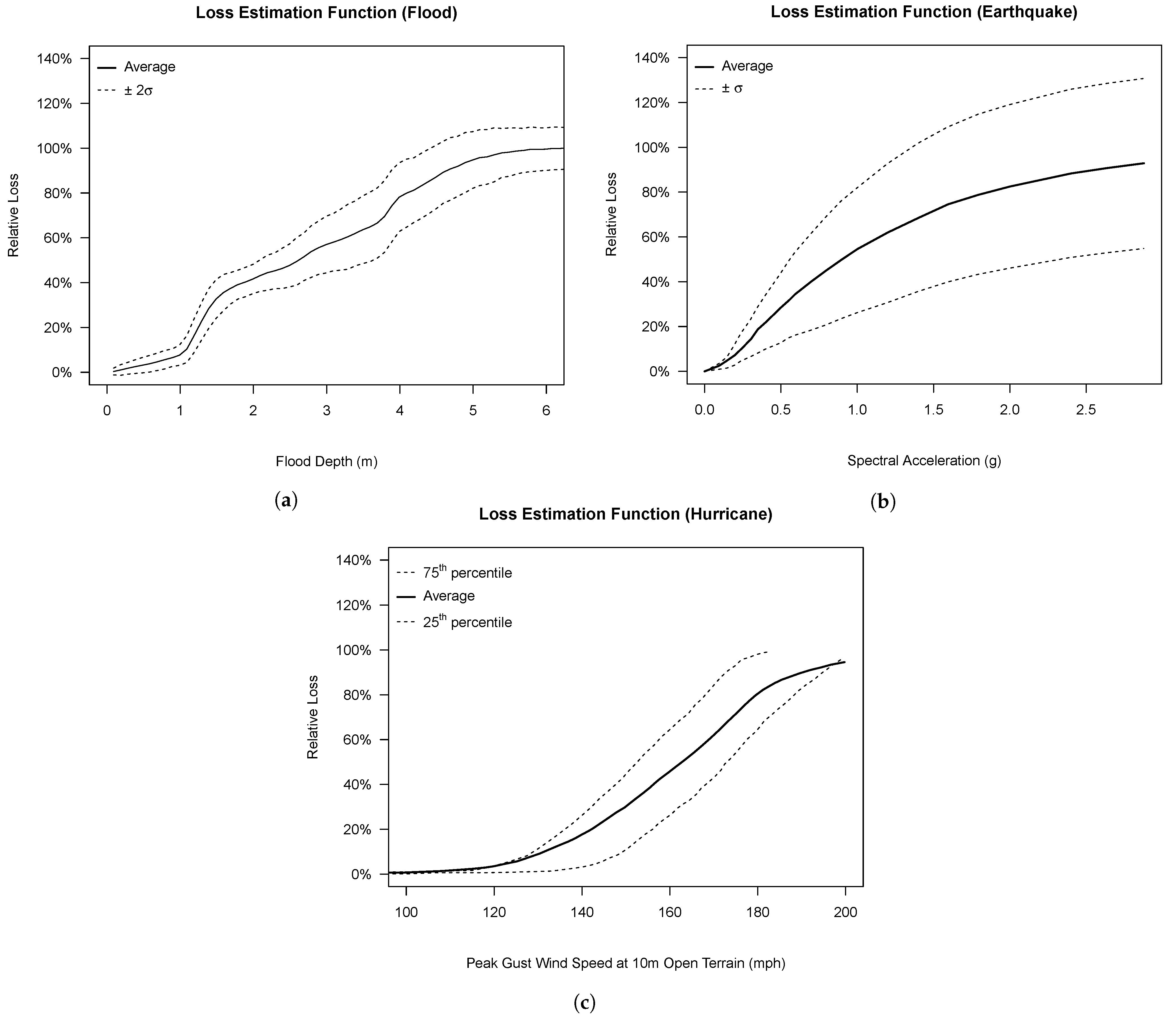
The size of the loss for an individual building in a Nat Cat event dependents on the physical characteristics of the building (structural properties, construction material, floor plan, etc.) and the hazard intensity at the building location (magnitude of energy and forces applied to the structure). For a specific type of building (a building with specific physical characteristics), the loss estimation function presents the relationship between the loss size of a building and the intensity of a specific natural hazard at the property location. In a loss estimation function, the loss size is defined as the ratio of the loss to the total value of the property (relative loss). The physical characteristics are captured by categorizing buildings into different classes with a similar response to the hazard. One or more intensity measures of the hazard are used to describe how the loss ratio changes as the intensity increases at the property location.

For instance, the loss estimation function for flood is called depth-damage function as the depth of flood at the building location is commonly used as the sole intensity measure for flood damage estimation (Marvi 2020). The depth-damage function describes how flood damage (relative to the property value) increases as the flood water height increases at the building location. Different depth-damage functions have been developed for different types of buildings to capture the role of physical characteristics. Figure 1 illustrates examples of loss estimation functions for flood, earthquake, and hurricane.

The loss estimation function of a building is composed of two parts: (1) a deterministic non-decreasing trend which is the function of the hazard intensity at the building location, $g\left(\mathit{X}\right)$; (2) a stochastic term with a variance that may change by the hazard intensity, ${\sigma }_{\mathit{X}}\epsilon$. Here, $\mathit{X}$ represents the intensity of a natural hazard that the loss estimation function of the building is constructed for. Since the intensity of a natural hazard varies in a region, note that $\mathit{X}$ is the local evaluation of the intensity measure at the property location. For simplicity, we follow the general assumption that the random variable $\epsilon$ has a standard normal distribution, and ${\sigma }_{\mathit{X}}$ is the standard deviation of the loss given the intensity of $\mathit{X}$ around its average value or $g\left(\mathit{X}\right)$. Thus, for a specific natural hazard, the building i in a region will have a random loss of $L_i$ as

$$L_i=g_i\left({\mathit{X}}_i\right)+{\sigma }_{{\mathit{X}}_i}\epsilon ,$$

(1)

when the intensity measures of the hazard are evaluated as the vector ${\mathit{X}}_i$ at the property location.

2.2.1. Source of Correlation

Intensity of a natural hazard varies spatially, yet is correlated. The variability of the intensity in a region can be described by the physics model governing the natural phenomenon and the event parameters as the initial values and/or boundary conditions of such a model. For example, flood water height, as an intensity of flood, can be determined in an entire region by the governing hydraulic model calibrated for that specific region, and the river water level at the upstream of the region is the only event parameter required in this model. In this example, the intensity measure of the hazard and the event parameter are from the same quantity; both are height and measured by the same unit. However, the intensity measure and the event parameters can be different in number and quantity. The physics model specifies the event parameters required for the estimation of the intensity in a region. As the natural phenomenon occurs with random magnitude, the event parameters representing such magnitude will be a set of random variables.

The calibrated hazard model determines the intensity in any part of the region including at building locations using some event parameters. Assume that the hazard model calibrated for a region is known and denoted by a deterministic function $\mathcal{D}$; the event parameters required for the hazard model are denoted by the vector $\mathsf{\Theta }$; and, the location of the building i in the region is used in the hazard model in the form of the vector ${\mathit{z}}_i$. Thus, ${\mathit{X}}_i$ can be determined by

$${\mathit{X}}_i=\mathcal{D}\left({\mathit{z}}_i;\mathsf{\Theta }\right),$$

(2)

where the ${\mathit{X}}_i$’s are all dependent on the event parameters $\mathsf{\Theta }$ through the deterministic physics model $\mathcal{D}$ and the buildings’ fixed geographical location ${\mathit{z}}_i$. Note that $\mathcal{D}$ for any ${\mathit{z}}_i$’s is non-decreasing as $\mathsf{\Theta }$ changes to the event parameters representing a less frequent event (an event with lower exceedance probability). Thus, ${\mathit{X}}_i$’s and consequently $g_i\left({\mathit{X}}_i\right)$’s become correlated. Note that the functions $g_i(.)$ are non-decreasing. Furthermore, ${\mathit{X}}_i$’s are non-decreasing as the intensity of the hazard increases. Thus, the correlation among building losses are positive and can be traced back to the event intensity which is captured by parameters in $\mathsf{\Theta }$. Given a specific hazard intensity $\left({\mathit{X}}_i\right)$, the part $g_i\left({\mathit{X}}_i\right)$ is a deterministic term of the building loss which we call it systematic loss. The stochastic term of the building loss, ${\sigma }_{{\mathit{X}}_i}\epsilon$, is uncorrelated among the buildings of the region, and we call it residual loss. Thus, the residual risk is idiosyncratic and insurable.

The correlated systematic part of the loss for the individual buildings can be aggregated and considered the systematic loss of the region as

$$L^s={\sum }_{i=1}^N{g}_i\left({\mathit{X}}_i\right)={\sum }_{i=1}^N{g}_i\left(\mathcal{D}\left({\mathit{z}}_i;\mathsf{\Theta }\right)\right)=G\left(\mathsf{\Theta }\right),$$

(3)

where $L^s$ represents the systematic loss of the region assuming that there are N buildings in the region (or in our portfolio). Since the location of the buildings (${\mathit{z}}_i$), their structural characteristics (captured by $g_i\left(.\right)$), and the hazard model of the region (captured by $\mathcal{D}\left(.\right)$) do not change, the $L^s$ is a deterministic function of $\mathsf{\Theta }$. So, we can simplify Equation (3) to $L^s=G\left(\mathsf{\Theta }\right)$. Likewise, the residual loss of the region ($L^r$) is defined by the sum of the residual losses of the buildings in the region as in

$$L^r={\sum }_{i=1}^N{\sigma }_{{\mathit{X}}_i}\epsilon \sim \mathcal{N}\left(0,\sqrt{{\sum }_{i=1}^N{\sigma }_{{\mathit{X}}_i}^2}\right)\mathrm{or}\mathcal{N}\left(0,{\sigma }_{\mathsf{\Theta }}\right).$$

(4)

Note that $L^r$ is a random variable which is a sum of N normally distributed random variables. Thus, $L^r$ is a normal random variable with $E\left(L^r\right)=0$ and $Var\left(L^r\right)={\sum }_{i=1}^N{\left({\sigma }_{{\mathit{X}}_i}\right)}^2$. For simplicity, we use ${\sigma }_{\mathsf{\Theta }}$ to show the standard deviation of $L^r$. The total loss of the region (L) is the sum of the losses for all the buildings in the region which is equal to the sum of the systematic and the idiosyncratic residual loss of the region as explained in

$$L={\sum }_{i=1}^N{L}_i={\sum }_{i=1}^N{g}_i\left({\mathit{X}}_i\right)+{\sum }_{i=1}^N{\sigma }_{{\mathit{X}}_i}\epsilon =L^s+L^r.$$

(5)

2.2.2. Risk Decomposition

The systematic part of the natural catastrophe risk, $L^s$, can be transferred to the capital markets by issuing parametric CAT bonds. For this reason, the range of $\mathsf{\Theta }$ is divided into J mutually exclusive and collectively exhaustive subdomains, ${\mathsf{\Theta }}_j$ for $j=1,\dots ,J$. The subdomains are constructed in a way that any event in ${\mathsf{\Theta }}_k$ has an annual exceedance probability less than any event in ${\mathsf{\Theta }}_h$ if and only if $k>h$. The annual exceedance probability of the natural phenomenon is assumed to be known in the region using historical measurements of $\mathsf{\Theta }$ and statistical estimation methods such as extreme value theory. For the subdomain ${\mathsf{\Theta }}_j$, a parametric CAT bond $B_j$ is issued with a total principal as its collected asset invested in a trust which is equal to $b_j$ described in

$$b_j=\left\{\begin{array}{cc}E\left[G\left(\mathsf{\Theta }\right)\left|\mathsf{\Theta }\in {\mathsf{\Theta }}_1\right.\right],\hfill & j=1,\hfill \\ E\left[G\left(\mathsf{\Theta }\right)\left|\mathsf{\Theta }\in {\mathsf{\Theta }}_j\right.\right]-b_{j-1},\hfill & j\ne 1,\hfill \end{array}\right.\mathrm{for}j=1,\dots ,J.$$

(6)

Like other bonds, the parametric CAT bond pays interest in the form of coupons; however, the principal and maybe the interest will be withdrawn if the triggering event occurs. Here, we assume that the parametric CAT bond $B_j$ is paying interest with an annual rate of ${\alpha }_j$, and the whole principal will be withdrawn in case the bond is triggered. An event with the intensity ${\mathsf{\Theta }}_0$ triggers the parametric CAT bond $B_j$, if there exists at least one event in ${\mathsf{\Theta }}_j$ with the annual exceedance probability greater than the annual exceedance probability of ${\mathsf{\Theta }}_0$. Since the annual exceedance probability for $\mathsf{\Theta }$ is known with a consensus among the involved parties (insurer and investors), and ${\mathsf{\Theta }}_0$ is measured fairly quickly by objective third parties (such as government agencies like USGS and NOAA), the involved parties will have an identical recognition in a short time whether the bond has been triggered or not. This increases transparency and helps to release the bond asset quickly to cover the losses from the event.

By transferring the systematic risk to the capital markets, the remaining part of the risk (the residual risk) becomes idiosyncratic and hence insurable. Assume that the event with ${\mathsf{\Theta }}_0$ triggers the parametric CAT bonds $B_1,\dots ,B_s$. The total fund provided by the triggered bonds equals to

$$b_0={\sum }_{i=1}^s{b}_i=E\left[G\left(\mathsf{\Theta }\right)\left|\mathsf{\Theta }\in {\mathsf{\Theta }}_s\right.\right].$$

(7)

Thus, the remaining part of the loss is $\left[G\left({\mathsf{\Theta }}_0\right)-b_0\right]+L^r$. It is assumed that ${\mathsf{\Theta }}_j$’s are small enough that the variability of $\left[G\left({\mathsf{\Theta }}_0\right)-b_0\right]$ is negligible compare to the variability of $L^r$. In other words, the total loss (L) is not sensitive to the variability of $G\left(\mathsf{\Theta }\right)$ around its conditional average $E\left[G\left(\mathsf{\Theta }\right)\left|\mathsf{\Theta }\in {\mathsf{\Theta }}_s\right.\right]$. As shown in Equation (4), conditional on the realization of $\mathsf{\Theta }$, the residual risk has a normal distribution with standard deviation ${\sigma }_{\mathsf{\Theta }}$. Thus, the residual risk, denoted by $L^r$, has a compound normal distribution as described in

$$\begin{array}{c}{L}^r\sim \mathcal{N}\left(0,{\sigma }_{\mathsf{\Theta }}\right),\\ Pr\left({\sigma }_{\mathsf{\Theta }}\right)\mathrm{is}\mathrm{known}\mathrm{through}Pr\left(\mathsf{\Theta }\right),\end{array}$$

(8)

Instead of using a compound distribution, a conservative or risk averse option is to use the maximum ${\sigma }_{\mathsf{\Theta }}$ over possible $\mathsf{\Theta }$ as the standard deviation of the residual risk $L^r$. One can add an extra dispersion to ${\sigma }_{\mathsf{\Theta }}$ for considering the variability of $G\left(\mathsf{\Theta }\right)$ around its conditional average over ${\mathsf{\Theta }}_j$’s intervals. In that case, the modified standard deviation (${\sigma }_{\mathsf{\Theta }}^m$) used for the normal distribution of $L^r$ is calculated by

$${\sigma }_{\mathsf{\Theta }}^m=\sqrt{{\sigma }_{\mathsf{\Theta }}^2+{\sum }_{j=1}^{k}Var\left[G\left(\mathsf{\Theta }\right)\left|\mathsf{\Theta }\in {\mathsf{\Theta }}_j\right.\right]},$$

(9)

where k is the highest index of the bonds triggered if an event with the intensity of $\mathsf{\Theta }$ occurs.

2.2.3. Nat Cat Premium Calculation

Premium collected from individual buildings needs to cover the costs including a portion of the CAT bond interest, the residual risk, and the underwriting gain. Those costs should be distributed fairly among the individual buildings. The CAT bond interest is partially provided from low-risk investments such as government or AAA corporate bonds and partially from the insureds’ premium. Assume that $I_j$ is the total interest that needs to be provided from insurance premiums for the CAT bond $B_j$. As the CAT bond is issued to cover the systematic part of the risk, it would be fair if $I_j$ is distributed among the individual buildings proportional to their average systematic risk within ${\mathsf{\Theta }}_j$. Thus, we define $c_{ij}^I$ as the portion of $I_j$ paid by the property i, and calculate $c_{ij}^I$ using

$$c_{ij}^I=\left\{\begin{array}{cc}\frac{E\left[g_i\left(\mathcal{D}\left({\mathit{z}}_i;\mathsf{\Theta }\right)\right)\left|\mathsf{\Theta }\in {\mathsf{\Theta }}_1\right.\right]}{b_1},\hfill & j=1,\hfill \\ \frac{E\left[g_i\left(\mathcal{D}\left({\mathit{z}}_i;\mathsf{\Theta }\right)\right)\left|\mathsf{\Theta }\in {\mathsf{\Theta }}_j\right.\right]-E\left[g_i\left(\mathcal{D}\left({\mathit{z}}_i;\mathsf{\Theta }\right)\right)\left|\mathsf{\Theta }\in {\mathsf{\Theta }}_{j-1}\right.\right]}{b_j},\hfill & j\ne 1,\hfill \end{array}\right.\mathrm{for}i=1,\dots ,N\mathrm{and}j=1,\dots ,J.$$

(10)

The residual risk is managed by the insurer based on variety of factors including the industry regulations, market competition, and company’s risk appetite. Based on all factors and the residual risk distribution mentioned in Equation (8), assume that the insurer decides to collect the total of V amount from the insured buildings to cover the residual risk. As the residual risk is more induced by the dispersion of the loss around its average, a fair practice to distribute V among the insureds is to find the contribution of each property to the total dispersion. Thus, we propose to use $c_i^V$ as the portion of V paid by the property i which is explained by

$$c_i^V=\frac{1}{Pr\left(\mathsf{\Theta }\in {\cup }_1^J{\mathsf{\Theta }}_j\right)}E\left[\frac{{\sigma }_{{\mathit{X}}_i}^2}{{\sigma }_{\mathsf{\Theta }}^2}\right]=\frac{1}{Pr\left(\mathsf{\Theta }\in {\cup }_1^J{\mathsf{\Theta }}_j\right)}E\left[\frac{{\sigma }_{g_i\left(\mathcal{D}\left({\mathit{z}}_i;\mathsf{\Theta }\right)\right)}^2}{{\sigma }_{\mathsf{\Theta }}^2}\right].$$

(11)

The underwriting gain is assumed to be a fixed rate of each policy. Assume that U is the total underwriting gain, and $q_i$ is the total portion of the premium paid by the building i for the CAT bond interest and its residual risk. So, the portion of U paid by the building i is denoted by $c_i^U$ and calculated using

$$\begin{array}{ccc}\hfill c_i^U& =& \frac{q_i}{{\sum }_{i=1}^N{q}_i}\hfill \\ \hfill q_i& =& {\sum }_{j=1}^J{c}_{ij}^I{I}_j+c_i^{V}V\hfill \end{array}\mathrm{for}i=1,\dots ,N.$$

(12)

Ultimately, the total premium needs to be collected from the building i is the sum of its portions from the CAT bond interest, residual risk, and underwriting gain. The total premium is denoted by $Q_i$ and calculated as

$$Q_i={\sum }_{j=1}^J{c}_{ij}^I{I}_j+c_i^{V}V+c_i^{U}U=q_i\left(1+\frac{U}{{\sum }_{i=1}^N{q}_i}\right)$$

(13)

2.2.4. CAT Bond Portfolio Measures

As a risky investment, the parametric CAT bonds are compared with other investment opportunities using their risk-return trade-off. Expected return and standard deviation of the returns are commonly used in risk-return trade-off to compare risky investments and quantify their risk. From two investments with the same expected return, the one with lower standard deviation (lower risk) is more favorable. Likewise, from two investments with the same standard deviation (same risk), the one with higher expected return is more favorable. The parametric CAT bond $B_j$ with a total principal of a generates a stochastic returns with their associated probabilities as

$$R_{1/\beta }=\left\{\begin{array}{cc}a\left(1+\alpha \right),\hfill & 1-\beta ,\hfill \\ -a\left(1-\delta \alpha \right),\hfill & \beta .\hfill \end{array}\right.$$

(14)

Here, $\alpha$ is the bond’s annual interest rate; $\delta$ determines the portion of the interest that is paid if the triggering event occurs. Note that $\delta =0$ if nothing is paid when the triggering event occurs, and $\delta =1$ if full interest is paid no matter the triggering event occurs. Finally, $\beta$ is the highest annual exceedance probability of the events in $B_j$. This means that any event with an annual exceedance probability less than $\beta$ will trigger the bond $B_j$. Thus, the bond $B_j$ can be named as $\beta$-bond or, with using return period instead of $\beta$, it can be named as $1/\beta$-year bond. For example, $B_j$ corresponding to $\beta =0.005$ is called 200-year bond. One can describe R using a Bernoulli random variable W with $P\left(W=0\right)=\beta$ and $P\left(W=1\right)=1-\beta$ as presented by

$$R_{1/\beta }=a\left(1+\alpha \right)W-a\left(1-\delta \alpha \right)\left(1-W\right)=a\left[2+\left(1-\delta \right)\alpha \right]W-a\left(1-\delta \alpha \right).$$

(15)

The expected value and standard deviation of the stochastic return $R_{1/\beta }$ is presented as

$$\begin{array}{c}{\mu }_{R_{1/\beta }}=a\left[1+\alpha -\left[2+\left(1-\delta \right)\alpha \right]\beta \right],\\ {\sigma }_{R_{1/\beta }}=a\left[2+\left(1-\delta \right)\alpha \right]\sqrt{\beta \left(1-\beta \right)}.\end{array}$$

(16)

Thus, the results for special cases of $\delta =0$ and $\delta =1$ are derived, respectively, as follows

$$\begin{array}{c}{\mu }_{R_{1/\beta }}=a\left[1+\alpha -\left[2+\alpha \right]\beta \right],\\ {\sigma }_{R_{1/\beta }}=a\left[2+\alpha \right]\sqrt{\beta \left(1-\beta \right)}.\end{array}\mathrm{for}\delta =0$$

(17)

$$\begin{array}{c}{\mu }_{R_{1/\beta }}=a\left[1+\alpha -2\beta \right],\\ {\sigma }_{R_{1/\beta }}=2a\sqrt{\beta \left(1-\beta \right)}.\end{array}\mathrm{for}\delta =1$$

(18)

CAT bond interest is paid by a set of coupons of the same amount throughout the year. For example, a bond with principal value of a, annual interest rate $\alpha$, and quarterly-paid coupons pays $\left(1/4\right)a\alpha$ at the end of each quarter. In the case of a CAT bond, the payment is made if the bond had not been triggered before the coupon is due. As soon as the triggering event occurs, the bond releases the fund to cover the losses, and there would be no asset to generate interest anymore; consequently, the remaining coupon payments will be canceled. Assume an investor is holding a CAT bond with the maturity of one year, the annual interest rate of $\alpha$, and the interest paid by T coupon payments during the year. In the case that the triggering event occurs, the total interest received by the investor can have T different amounts depending on when the triggering event occurs and cancels the remaining coupons.

Table 3. Interest received by the investors if the triggering event occurs.

Earliest Coupon Canceled	1st	2nd	⋯	tth	⋯	Tth
Total interest received	0	$\left(1/T\right)a_1\alpha$	⋯	$\left((t-1)/T\right)a_1\alpha$	⋯	$\left((T-1)/T\right)a_1\alpha$
Equivalent $\delta$	0	$1/T$	⋯	$(t-1)/T$	⋯	$(T-1)/T$

describes the total interest an investor receives based on the time the triggering event occurs during the CAT bond’s maturity year. The equivalent $\delta$ for each case is also presented in Table 3.

If the investor has a belief that the triggering event occurs with a certain likelihood throughout the year, their view for the expected value and standard deviation of the returns of the parametric CAT bond can be updated accordingly. Assume that the investor believes if the triggering event occurs, it occurs at a time between $(t-1)$th and tth coupon payments with the probability of $Pr\left({\delta }_t\right)$, for $t=1,\dots ,T$ and the 0th coupon payment as the beginning of the CAT bond contract. So, the investor’s updated view can be described by

$$\begin{array}{ccccc}\hfill {\mu }_{R_{1/\beta }}& =& {\sum }_{t=1}^T\left({\mu }_{R_{1/\beta }\left|{\delta }_t\right.}\right)Pr\left({\delta }_t\right)\hfill & =& a\left[1+\alpha -\left[2+\left(1-{\mu }_{\delta }\right)\alpha \right]\beta \right],\hfill \\ \hfill {\sigma }_{R_{1/\beta }}& =& \sqrt{{\sum }_{t=1}^T\left({\sigma }_{R_{1/\beta }\left|{\delta }_t\right.}^2\right)Pr\left({\delta }_t\right)}\hfill & =& a\left(\sqrt{{\left[2+\left(1-{\mu }_{\delta }\right)\alpha \right]}^2+{\sigma }_{\delta }^2{\alpha }^2}\right)\sqrt{\beta \left(1-\beta \right)}.\hfill \end{array}$$

(19)

2.3. Multi-Regional Parametric CAT Bond

The proposed parametric CAT bonds of different regions can be combined together and offered to investors as a single bond. Assume M different regions ($m=1,\dots ,M$) are exposed to natural hazards, and each region constructs parametric CAT bonds of $B_j^m$. The bonds with the same corresponding $\beta$ can form a single $1/\beta$-year bond (${\mathbb{B}}_{1/\beta }$) if the natural hazard occurs in any region independently from the others. Note that the natural hazards do not need to be of the same type; the parametric CAT bonds of the regions need to have the same $\beta$. The investment returns from such parametric CAT bond ${\mathbb{B}}_{1/\beta }$ is explained by

$${\mathbb{R}}_{1/\beta }={\sum }_{m=1}^M{\left(R_{1/\beta }\right)}_m={\sum }_{m=1}^M\left[a_m\left[2+\left(1-{\delta }_m\right){\alpha }_m\right]W_m-a_m\left(1-{\delta }_m{\alpha }_m\right)\right],$$

(20)

where $W_m$’s are i.i.d Bernoulli random variables. As ${\left(R_{1/\beta }\right)}_m$’s are portfolios with the same risk $\beta$, it is logical to assume that they have the same reward ${\alpha }_m=\alpha$. For simplicity, let us assume ${\delta }_m$ is constant and equal to $\delta$ for now. Since the bonds $B_j^m$’s should provide different amount of funds in case they are triggered, a unit investment in ${\mathbb{B}}_{1/\beta }$ needs to be distributed unevenly among the regions. If it is triggered, the bond $B_j^m$ will withdraw ${\eta }_m=b_0^m/{\sum }_{m=1}^M{b}_0^m$ of the total fund collected by ${\mathbb{B}}_{1/\beta }$. Note that the coefficients ${\eta }_m$, where ${\sum }_{m=1}^M{\eta }_m=1$, are the same for all investors and determined by the CAT bonds $B_j^m$’s constructing ${\mathbb{B}}_{1/\beta }$. Thus, an investor holding the parametric CAT bond ${\mathbb{B}}_{1/\beta }$ with the principal value of a has contributions to $B_j^m$ equal to $a_m={\eta }_{m}a$. Based on these assumptions and clarifications, Equation (20) can be simplified to

$${\mathbb{R}}_{1/\beta }=a\left[2+\left(1-\delta \right)\alpha \right]{\sum }_{m=1}^M\left[{\eta }_m{W}_m\right]-a\left(1-\delta \alpha \right).$$

(21)

Similar to the individual parametric CAT bonds, investors are interested to know the expected return and standard deviation of the returns for their investment on ${\mathbb{B}}_{1/\beta }$. An investor holding ${\mathbb{B}}_{1/\beta }$ with the principal value of a can calculate the expected value and standard deviation of their investment as

$$\begin{array}{ccc}\hfill {\mu }_{{\mathbb{R}}_{1/\beta }}& =& a\left[1+\alpha -\left[2+\left(1-\delta \right)\alpha \right]\beta \right],\hfill \\ \hfill {\sigma }_{{\mathbb{R}}_{1/\beta }}& =& a\left[2+\left(1-\delta \right)\alpha \right]\sqrt{\beta \left(1-\beta \right)}\sqrt{{\sum }_{m=1}^M{\eta }_m^2}.\hfill \end{array}$$

(22)

Since ${\eta }_m<1$ for $m=1,\dots ,n$, we can conclude that ${\eta }_m^2<{\eta }_m<1$ which means $\sqrt{{\sum }_{m=1}^M{\eta }_m^2}<\sqrt{{\sum }_{m=1}^M{\eta }_m}=1$. Comparing ${\mathbb{R}}_{1/\beta }$ with $R_{1/\beta }$, no surprise, the expected returns are the same; however, the standard deviation of ${\mathbb{R}}_{1/\beta }$ is less than the one for $R_{1/\beta }$ by the factor $\sqrt{{\sum }_{m=1}^M{\eta }_m^2}$. According to Chebyshev’s sum inequality, $\sqrt{{\sum }_{m=1}^M{\eta }_m^2}$ reaches its lowest value at $1/\sqrt{M}$ when ${\eta }_m$’s are all equal which means ${\eta }_m=1/M$ for $m=1,\dots ,n$. Investment on ${\mathbb{B}}_{1/\beta }$ with returns ${\mathbb{R}}_{1/\beta }$ is more favorable than $B_{1/\beta }$ with returns $R_{1/\beta }$ due to its lower standard deviation of the returns.

If an investor has a belief about when, during the year, the triggering events may occur in the regions of the parametric CAT bond, the assumption about ${\delta }_m$ being constant and equal for all m’s can be relaxed, and the expected return and standard deviation of the returns can be updated accordingly. Given a set of ${\delta }_m$’s and considering ${\xi }_m=\left[2+\left(1-{\delta }_m\right)\alpha \right]$, Equation (21) can be written as

$${\mathbb{R}}_{1/\beta }\left|{\delta }_m\right.=a{\sum }_{m=1}^M\left[{\xi }_m{\eta }_m{W}_m\right]-a\left(1-\alpha {\sum }_{m=1}^M{\delta }_m\right).$$

(23)

Assume $\Delta$ includes all possible combinations for ${\delta }_m$ with their associated probabilities. Hence, ${\mu }_{{\mathbb{R}}_{1/\beta }}$ and ${\sigma }_{{\mathbb{R}}_{1/\beta }}$ can be derived using

$$\begin{array}{ccc}\hfill {\mu }_{{\mathbb{R}}_{1/\beta }}& =& {\sum }_{\Delta }\left[{\mathbb{R}}_{1/\beta }\left|{\delta }_m\right.\right]Pr\left({\delta }_m\right),\hfill \\ \hfill {\sigma }_{{\mathbb{R}}_{1/\beta }}& =& \sqrt{{\sum }_{\Delta }{\left[{\mathbb{R}}_{1/\beta }\left|{\delta }_m\right.\right]}^{2}Pr\left({\delta }_m\right)-{\mu }_{{\mathbb{R}}_{1/\beta }}^2}.\hfill \end{array}$$

(24)

2.4. Multi-Hazard Parametric CAT Bond

As different natural events, such as floods and earthquakes, occur independently in a region, their parametric CAT bonds can form a single portfolio similar to the CAT bonds of multiple regions. Like multi-regional parametric CAT bond, the parametric CAT bonds of different hazards in a region can construct a single bond as long as they have the same $\beta$. The expected return and standard deviation of the returns can be derived by the same logic and formulas explained for multi-regional parametric CAT bond.

As more regions and hazards are added, the parametric CAT bond becomes more diversified. Diversity helps to reduce the probability that a large number of the involved bonds are triggered. This allows the issuer to invest a portion of the collected principles in riskier investments than AAA government bonds for a higher return. It is even possible to collect less principle for the entire bond as the probability if all (or majority) of the bonds are triggered becomes extremely low. In addition, investors will accept lower interest rates as the parametric CAT bond becomes more diversified and thus less risky. So, the premiums can be reduced even more.

The probability distribution governing the parametric CAT bond ${\mathbb{R}}_{1/\beta }$ can be estimated using saddle-point approximation method (Butler 2007). The cumulant generating function (CGF) of ${\mathbb{R}}_{1/\beta }$ is required for saddle-point approximation which can be derived from Equation (21) or Equation (23). Thus, the CGF and its first three derivatives can be calculated as

$$\begin{array}{ccc}\hfill K\left(t\right)& =& M\beta -\mathsf{\Psi }t+\left(1-\beta \right){\sum }_{m=1}^M{e}^{{\gamma }_{m}t},\hfill \\ \hfill K^{\prime }\left(t\right)& =& -\mathsf{\Psi }+\left(1-\beta \right){\sum }_{m=1}^M{\gamma }_m{e}^{{\gamma }_{m}t},\hfill \\ \hfill K^{″}\left(t\right)& =& \left(1-\beta \right){\sum }_{m=1}^M{\gamma }_m^2{e}^{{\gamma }_{m}t},\hfill \\ \hfill K^{‴}\left(t\right)& =& \left(1-\beta \right){\sum }_{m=1}^M{\gamma }_m^3{e}^{{\gamma }_{m}t},\hfill \end{array}$$

(25)

where

$$\mathsf{\Psi }=\left\{\begin{array}{cc}a\left(1-\delta \alpha \right),\hfill & \mathrm{for}{\mathbb{R}}_{1/\beta },\hfill \\ a\left(1-\alpha {\sum }_{m=1}^M{\delta }_m\right),\hfill & \mathrm{for}{\mathbb{R}}_{1/\beta }\left|{\delta }_m\right.,\hfill \end{array}\right.$$

and

$${\gamma }_m=\left\{\begin{array}{cc}a\left[2+\left(1-\delta \right)\alpha \right]{\eta }_m,\hfill & \mathrm{for}{\mathbb{R}}_{1/\beta },\hfill \\ a{\xi }_m{\eta }_m,\hfill & \mathrm{for}{\mathbb{R}}_{1/\beta }\left|{\delta }_m\right..\hfill \end{array}\right.$$

The saddle-point approximation for PDF and CDF of ${\mathbb{R}}_{1/\beta }$ at x are denoted by $\widehat{f}\left(x\right)$ and $\widehat{F}\left(x\right)$ presented, respectively, as follows

$$\widehat{f}\left(x\right)=\frac{1}{\sqrt{2\pi K^{″}\left(\widehat{s}\right)}}exp\left(K\left(\widehat{s}\right)-\widehat{s}x\right),$$

(26)

$$\widehat{F}\left(x\right)=\left\{\begin{array}{cc}\mathsf{\Phi }\left(\widehat{\omega }\right)+\varphi \left(\widehat{\omega }\right)\left(\frac{1}{\widehat{\omega }}-\frac{1}{\widehat{u}}\right),\hfill & \mathrm{for}x\ne \mu ,\hfill \\ \frac{1}{2}+\frac{K^{‴}\left(0\right)}{6\sqrt{2\pi }{K}^{″}{\left(0\right)}^{3/2}}=\frac{1}{2}+\frac{\left(1-\beta \right){\sum }_{m=1}^M{\gamma }_m^3}{6\sqrt{2\pi }{\left(1-\beta \right)}^{3/2}{\left({\sum }_{m=1}^M{\gamma }_m^2\right)}^{3/2}},\hfill & \mathrm{for}x=\mu ,\hfill \end{array}\right.$$

(27)

where $\widehat{s}$ is the solution to $K^{\prime }\left(\widehat{s}\right)=x$, $\widehat{\omega }=\mathrm{sgn}\widehat{s}\sqrt{2\left(\widehat{s}x-K\left(\widehat{s}\right)\right)}$, and $\widehat{u}=\widehat{s}\sqrt{K^{″}\left(\widehat{s}\right)}$.

For the case that ${\delta }_m$’s are not the same, the Equations (26) and (27) can be considered as the conditional PDF and CDF with respect to a set of ${\delta }_m$. Thus, the PDF and CDF of ${\mathbb{R}}_{1/\beta }$ can be determined using total probability rule over $\Delta$ as follows:

$$\begin{array}{ccc}\hfill \widehat{f}\left(x\right)& =& {\sum }_{\Delta }\widehat{f}\left(x\left|{\delta }_m\right.\right)Pr\left({\delta }_m\right),\hfill \\ \hfill \widehat{F}\left(x\right)& =& {\sum }_{\Delta }\widehat{F}\left(x\left|{\delta }_m\right.\right)Pr\left({\delta }_m\right).\hfill \end{array}$$

(28)

3. Illustrative Example

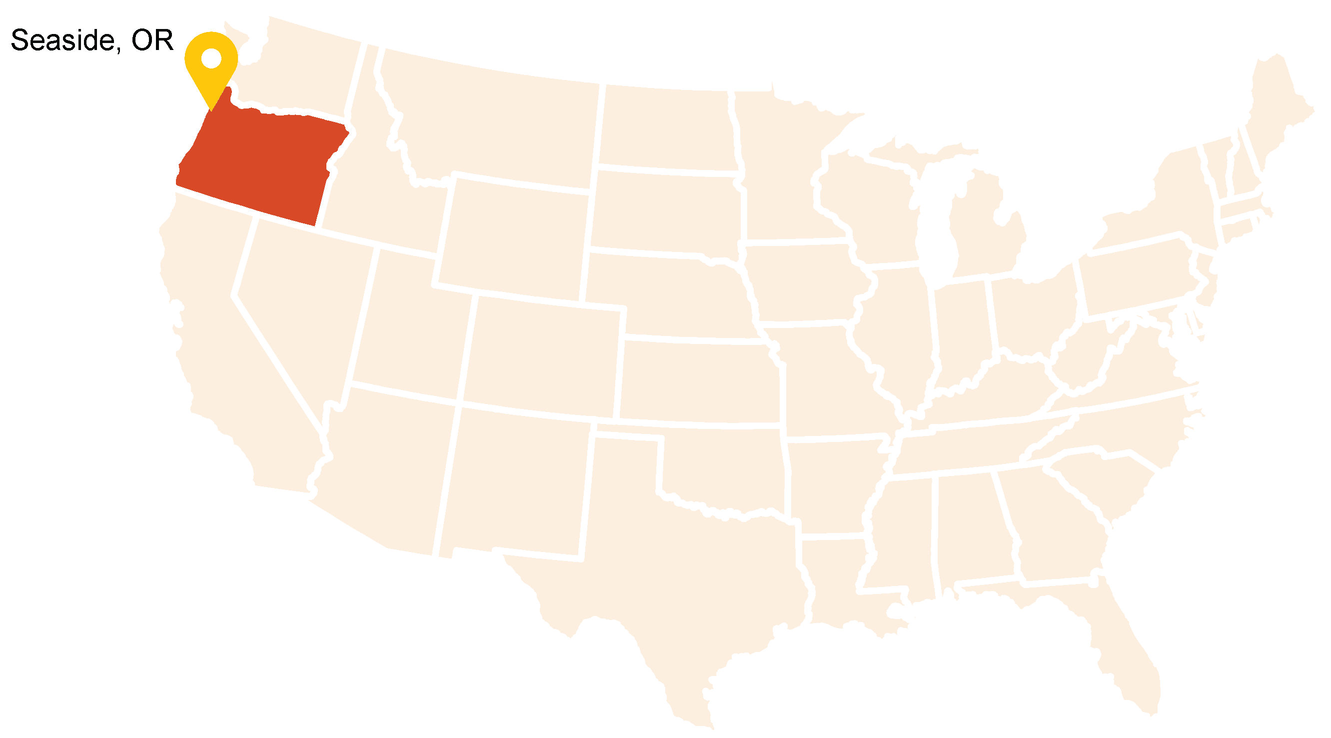
A part of the city of Seaside, Oregon is chosen to apply the proposed methodology for residential buildings subject to flood hazard. The city is in Clatsop County, the north east of Oregon State in the US. The location of the city on the US map is shown in Figure 2. The city has a total area of $3.92$ sq mi and serves about 6892 residents (estimate for 2019) (US Census Bureau 2019). Necanicum river and Neawanna creek flow through the city and divide it into three parts: west (of Necanicum river), middle (between the river and the creek), and east (of the Neawanna creek). Flood risk for the residential buildings in the west and middle regions is studied in this example.

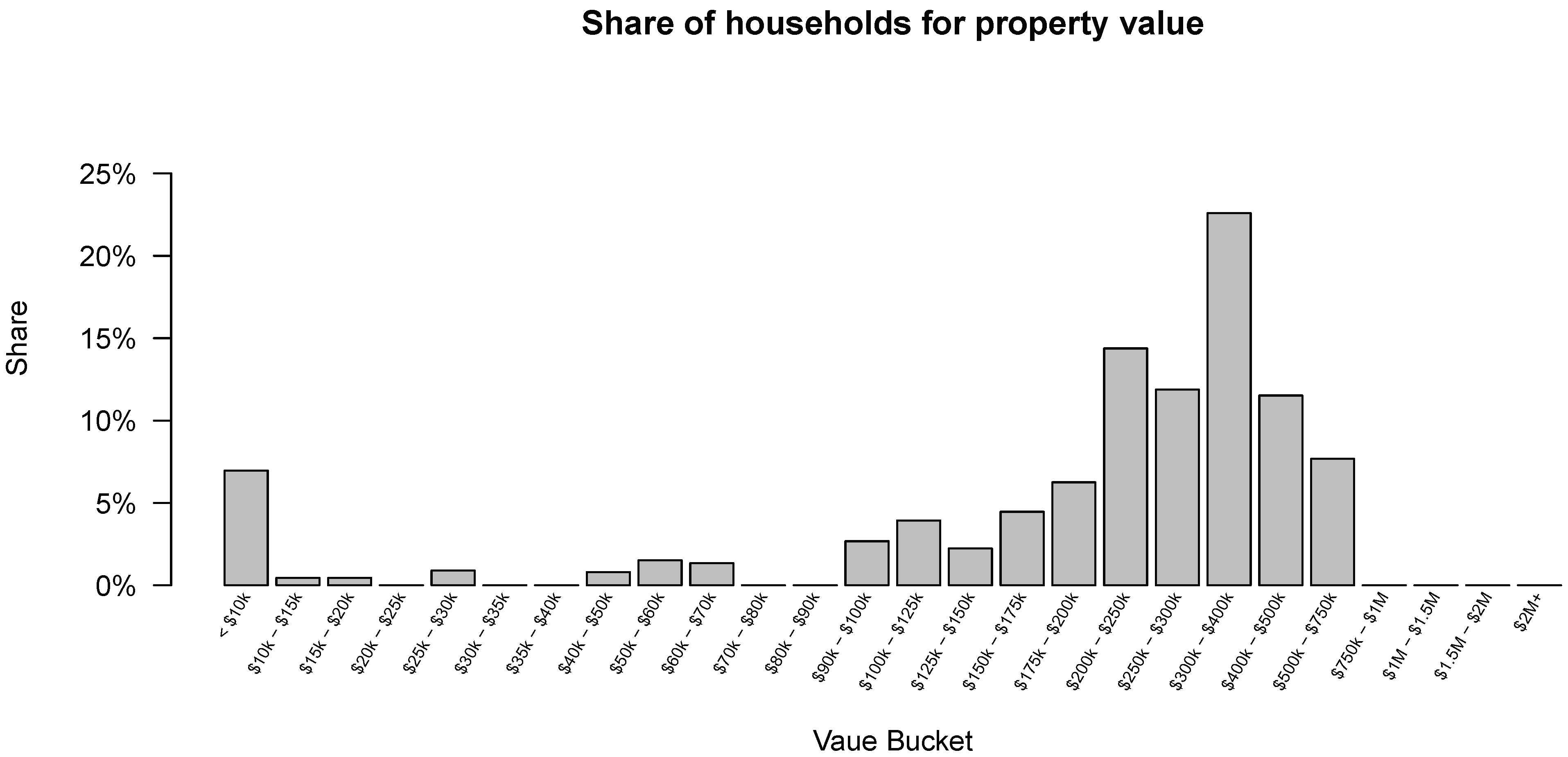
Building information required to estimate flood risk includes location (${\mathit{z}}_i$), total value, and depth-damage function as the loss estimation function (which means ${\mathit{X}}_i$ is the flood water depth at the location of building i or simply ${\mathit{X}}_i\to h_i$). The information can be acquired from various public and private sources such as municipal authorities and structural engineering firms. In this example, the location data is scraped from OpenStreetMap for some buildings in the study region, and the missing buildings are replaced using Google Satellite View. The buildings’ location and layout are stored as GIS polygon data in shapefile format which provides floor area of the buildings, too. A property value is assigned to each building based on its floor area in which buildings with larger areas are assumed to be more valuable. The assigned values are selected as to preserve the property value distribution of Seaside reported by Data USA (2021). This distribution is presented in Figure 3.

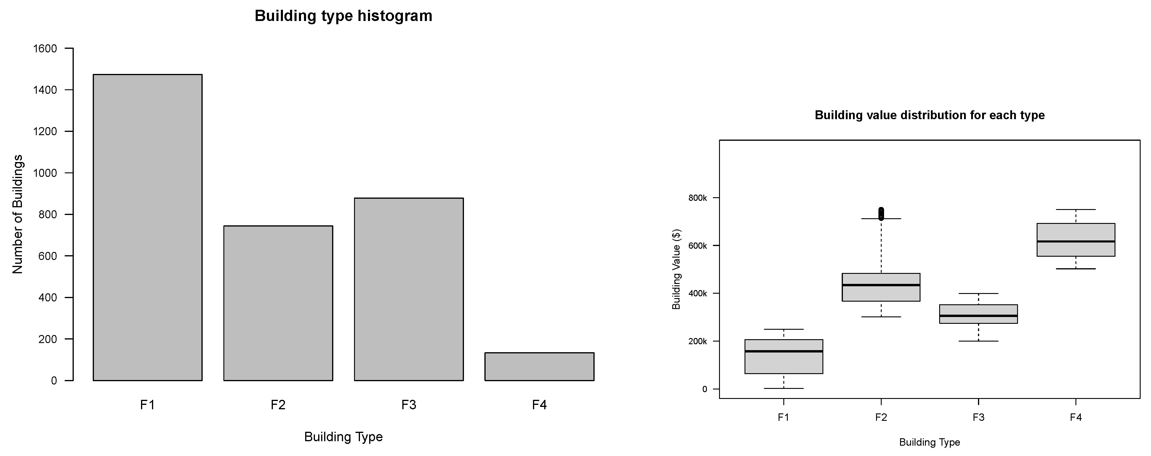
Depth-damage functions are chosen based on the type of building. In this study, we assume that the buildings in our risk portfolio are one of three types: (1) F1: One-story single-family residential building, (2) F2: One-story multi-family residential building, and (3) F3: Two-story single-family residential building. A type of building is assigned to each building, and its corresponding depth-damage function is adopted from Nofal and van de Lindt (2020). Figure 4 presents the histogram of building types and the distribution of building values in each type.

Flood risk for each building and the entire portfolio is calculated using a Monte Carlo simulation. Flood scenarios used in this study have return periods greater than or equal to 100 years. Losses from floods with a return period less than 100 years are supposed to be minimized by imposing restrictive building codes such as Flood Resistant Design and Construction (ASCE 2014). In addition, the US National Flood Insurance Program (NFIP) does not cover losses from floods with return periods less than 100 years (NFIP 2021). Thus, it is logical to only consider the losses generated from floods with return periods higher or equal to 100 years.

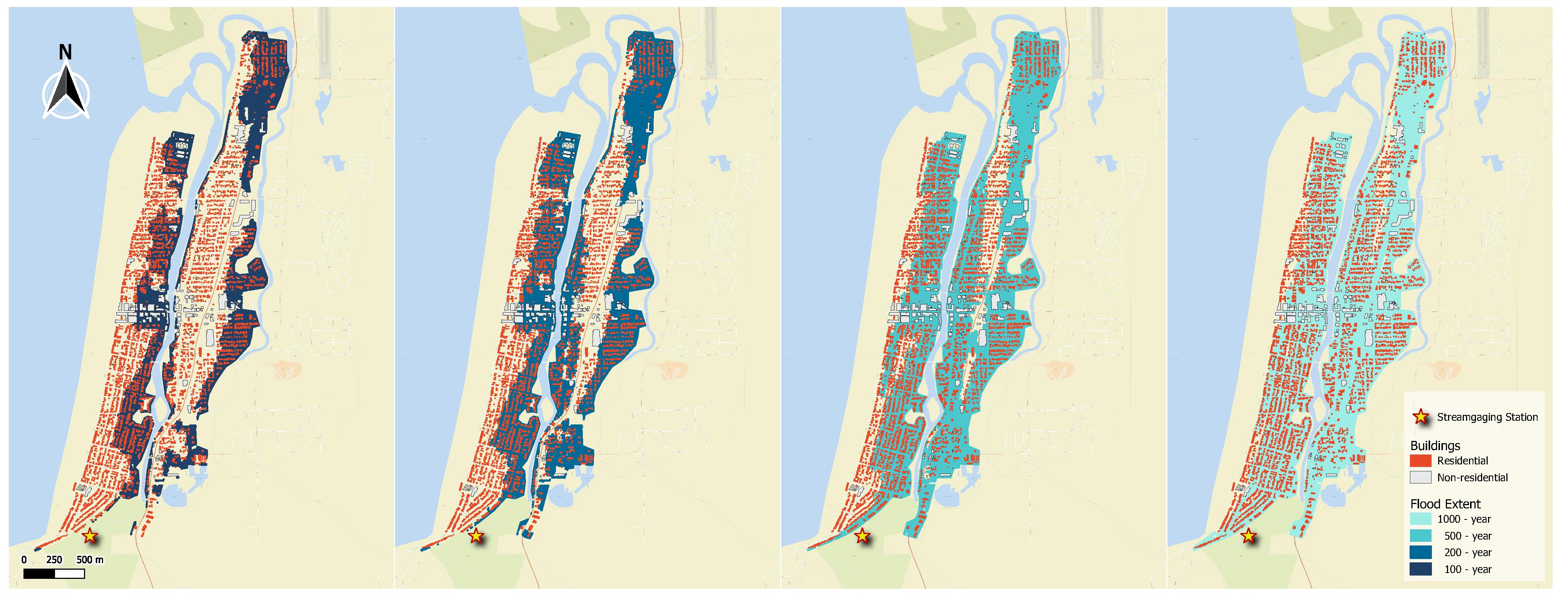
Flood scenarios are produced using water level at the upstream of Necanicum river. We assume that a streamgaging station exists at the upstream of Necanicum river which obtains a continuous record of the river water level. The location of this imaginary station is illustrated in Figure 5. It is common to calibrate a Generalized Extreme Value (GEV) distribution to characterize the exceedance probability distribution of a long-term (usually annual) water level of a river (Zervas 2013). Here, we assume that the annual exceedance probability of the river water level (h) follows a type II extreme value distribution (Fréchet) as

$$F\left(h;\mu ,\sigma ,\xi \right)=\left\{\begin{array}{cc}exp\left(-y^{-\alpha }\right),\hfill & y>0\hfill \\ 0,\hfill & y\le 0,\hfill \end{array}\right.$$

(29)

where $\xi =1/\alpha >0$ and $y=1+\xi \left(h-\mu \right)/\sigma$ with the parameters assumed as $\mu =2.7840$, $\sigma =0.31275$, and $\xi =0.176$. Based on this assumption, the corresponding water level for any return period can be derived. In this example, flood scenarios with return period greater than 100 years (equivalent to $5.0$ (m) water level at the station) are concerned. For a Monte Carlo simulation with $100,000$ year variants, the $5.0$ (m) water level at the station would be exceeded in $1000$ of the year variants. The return period of the events used in this study, their corresponding water levels, and their number of simulation in the Monte Carlo process are presented in

Table 4. The return period of the events, their corresponding water levels, and their number of simulations used in the study.

Return Period (yr)	100	115	132	151	172	195(≈200)	221	250	281	316	355
Water Level (m)	$5.0$	$5.1$	$5.2$	$5.3$	$5.4$	$5.5$	$5.6$	$5.7$	$5.8$	$5.9$	$6.0$
No. of Simulation	131	111	94	81	70	60	52	46	39	34	30
Cont’d	397	443	494(≈500)	549	610	676	747	825	909	1000	1205	1576
Cont’d	$6.1$	$6.2$	$6.3$	$6.4$	$6.5$	$6.6$	$6.7$	$6.8$	$6.9$	$7.0$	$7.2$	$7.5$
Cont’d	26	24	20	18	16	14	13	11	10	17	20	63

.

We assume that four parametric CAT bonds ($B_1$, $B_2$, $B_3$, and $B_4$) corresponding to the events with return periods of 100, 200, 500, and 1000 years, respectively, are used to decompose the risk in this region. Flood extension and depth of flood water in the entire study region can be derived using hydraulic modeling of the water flow in the river based on the water level at the station. Based on Equation (2), the hydraulic flow model represents $\mathcal{D}\left(.\right)$ that can determine the flood depth as the intensity of the flood at the location of the buildings ${\mathit{z}}_i$ by using the river water level at the station as the event parameter $\mathsf{\Theta }\to h$. The flood extension and the buildings flooded in each event are illustrated in Figure 5. To reduce the size of the calculations, we only consider the buildings in the west and middle parts of Seaside; a total of 2929 buildings.

A Monte Carlo simulation is conducted based on the flood events presented in Table 4. Based on Equation (2), for each flood event, the water depth around each building is determined using the flood map of the event, $h_i=\mathcal{D}\left({\mathit{z}}_i,h\right)$. Based on Equation (1), a set of possible losses for the building is randomly generated using the water depth ($h_i$) and the depth-damage function of the building. The number of the random losses in each event for each building is equal to the number of simulation mentioned in Table 4.

The total principal for each parametric CAT bond is calculated based on the realized losses using Equation (6). In this regard, $b_1$ is the average of the losses for the flood events with return periods 100, 115, 132, 151, and 172 years; $b_2$ is the average of the losses for the flood events with return periods 200, 221, 250, 281, 316, 355, 397, and 443 years subtracted by $b_1$; $b_3$ is the average of the losses for the flood events with return periods 500, 549, 610, 676, 747, 825, and 909 years subtracted by $b_2$; $b_4$ is the average of the losses for the flood events with return periods 1000, 1205, and 1576 years subtracted by $b_3$.

The residual risk of the losses for the region is calculated by finding $b_0$. For each event, $b_0$ is calculated using Equation (7). The total losses in each simulation subtracted by its corresponding $b_0$ gives the residual loss of that simulation. The distribution of the total losses and residual losses are the flood risk and the residual risk of the region. The same procedure can be applied for each individual building to obtain its flood risk and residual risk.

4. Results

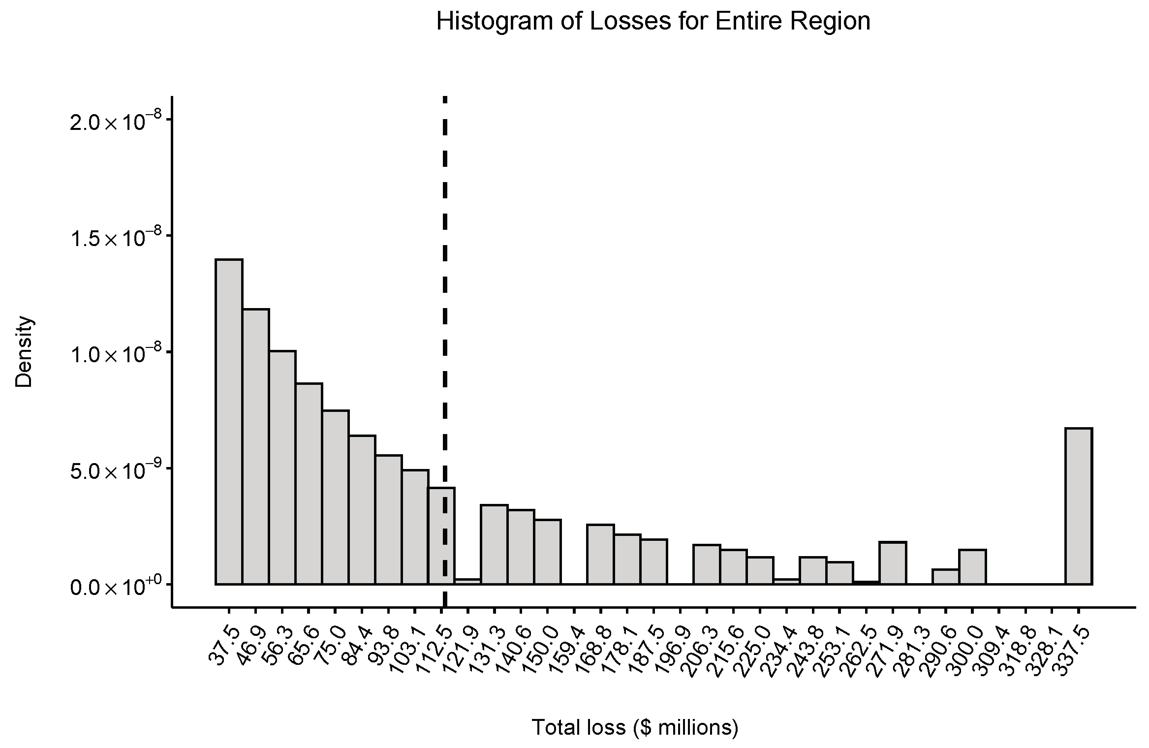
The simulation of the 1000 year variants produced 1000 total losses for each year. The histogram of those losses are considered as the conditional distribution of the flood loss given the return period of greater than 100 years. Figure 6 presents this distribution which is a heavy-tail exponential-like distribution as we expected. The average of the losses occurred around USD $113.8$ million (the vertical dashed line in Figure 6) and the standard deviation was USD $85.7$ million.

Based on the realized losses, the principal of the parametric CAT bonds were calculated and presented in

Table 5. The calculated CAT bond principals.

CAT Bond	${\mathit{B}}_1$	${\mathit{B}}_2$	${\mathit{B}}_3$	${\mathit{B}}_4$
Bond principal ($b_i$)	$\$51.9$ million	$\$61.9$ million	$\$97.0$ million	$\$105.0$ million
Spread interest rate	$4\%$	$3\%$	$2\%$	$1\%$
Bond total spread	$\$2.1$ million	$\$1.9$ million	$\$1.9$ million	$\$1.0$ million

. CAT bond interest can be divided into two parts: (1) the interest generated from the bond principle investing on a trust which is governed by risk-free rate, and (2) the spread of the catastrophe bond which is paid to the investors to compensate the involved risk. The bond spread is the portion of the interest that is covered by the insureds’ premium. To calculate this part for each building, an interest rate for each bond’s spread was assumed in this example which is presented in Table 5. The riskier the investment (or the lower the return period of the underlying catastrophe of the bond) the higher the interest. Each bond’s total spread was calculated according to the assumed spread interest rate and the total bond’s principal. The total spread for each bond is presented in Table 5.

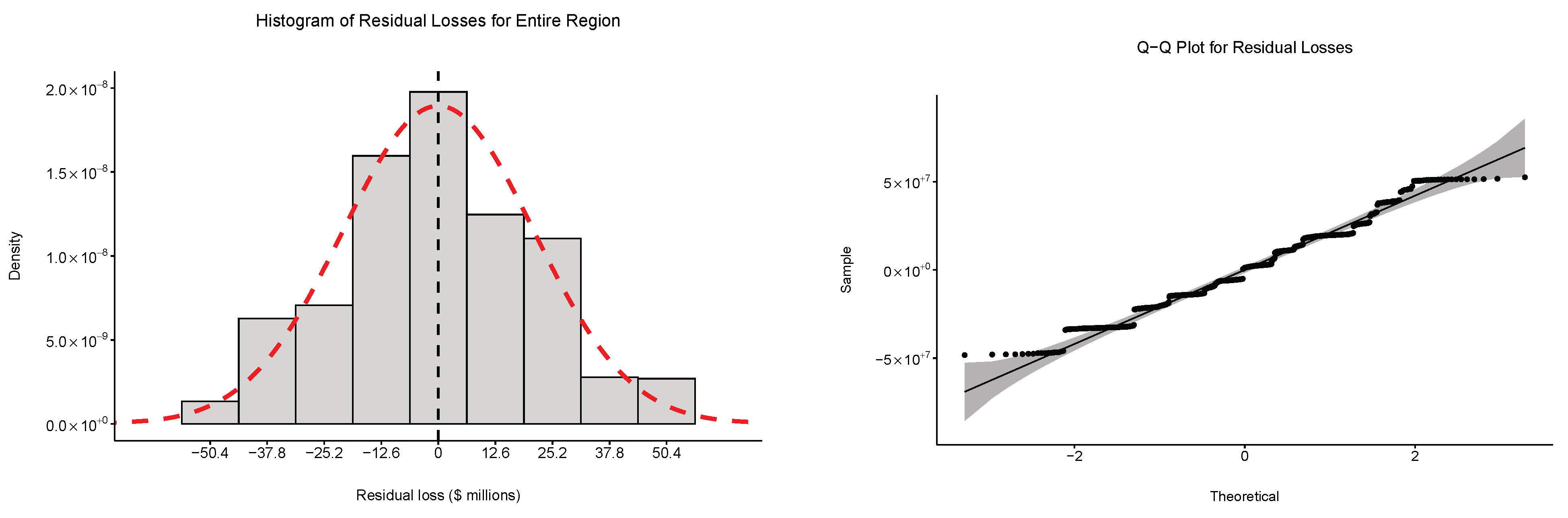
The residual losses for the simulated 1000 year variants were calculated by subtracting the triggered $b_i$’s from the total losses. The distribution of the residual losses is presented in Figure 7. The average of the residual losses occurred around zero (the vertical dashed line in Figure 7) and the standard deviation was USD $20.6$ million. The red dashed curve in Figure 7 shows a fitted normal density to the histogram of the residual losses. The Q-Q plot illustrated in Figure 7 verifies the normality of the residual losses.

The insurance premium for each building was calculated based on the results of this Monte Carlo simulation. The coefficients $c_{ij}^I$’s were calculated using Equation (10), and the bonds’ total spread were split and allocated to each building accordingly. We assumed that the total amount collected from the insureds to cover the residual risk is equivalent to the $70\%$ percentile of the residual risk distribution which was $V=$ USD $10.8$ million. The coefficients $c_i^V$’s were calculated using Equation (11), and V was distributed among the buildings according to $c_i^V$’s. Using Equation (12), $q_i$’s were calculated, and an assumed underwriting gain of $U=$ USD 1 million were distributed among the buildings accordingly. 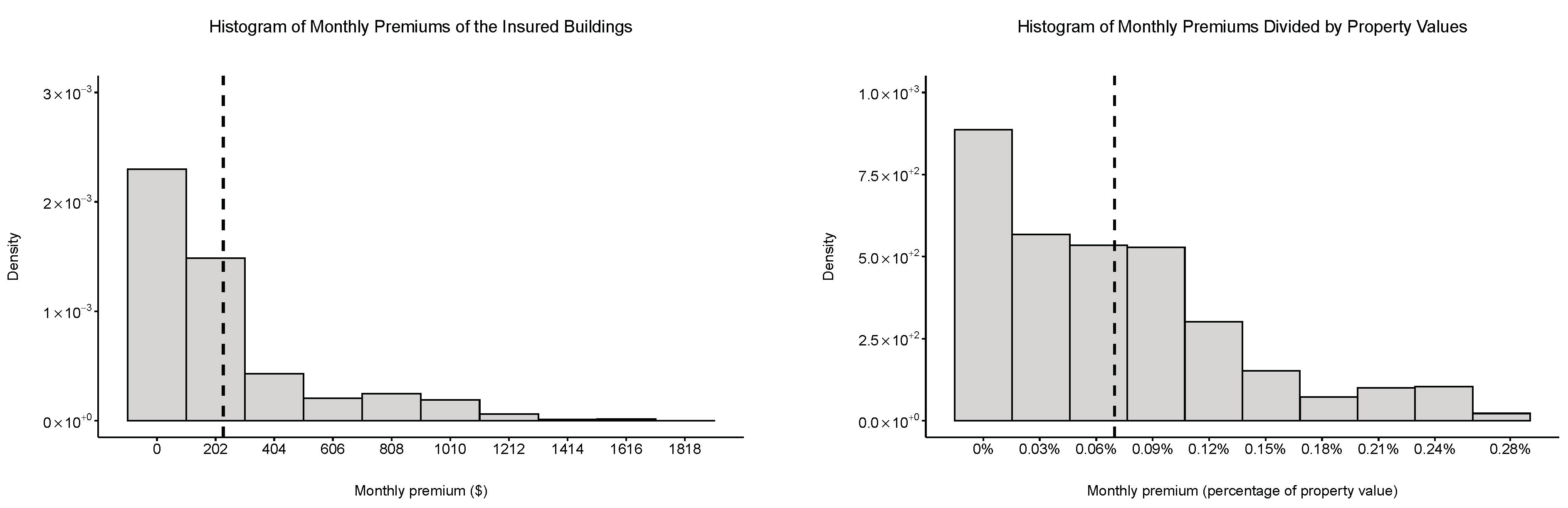Following Equation (13), $Q_i$ was derived as the total premium paid by each building. Figure 8 presents the histogram of the monthly premiums for each building as a dollar value and a percentage of the property value. The average dollar value of the monthly premiums was USD 230 with standard deviation USD 300, and the average percentage is $0.07\%$ with standard deviation $0.07\%$. A more detailed report for each building is accessible using a web app at https://mortezatm.shinyapps.io/RiskDecomposition/ (accessed on 16 November 2021).

5. Discussion

The result of the example demonstrates that the proposed methodology is able to fulfill its purposes including to transform the total loss distribution from a heavy-tail distribution into a normal distribution, and to provide an affordable insurance against a natural hazard to the households. To discuss those achievements, the distribution of the losses before and after decomposition are compared, and the affordability of the calculated premiums are investigated.

Comparing Figure 6 with Figure 7 shows that the decomposition could successfully transform the heavy-tail distribution of the total losses to the residual losses with a normal distribution. The losses before decomposition varies from USD $37.5$ million to USD $337.5$ million; while, the residual losses after decomposition varies from USD −50.4 million to USD $50.4$ million. This is a significant improvement to the loss distribution regarding insurance purposes.

The residual losses after the decomposition follow a normal distribution as shown in Figure 7; while, the losses before decomposition has a heavy-tail exponential-like distribution. As discussed in Section 2.1, losses with heavy-tail distributions are considered uninsurable. Thus, this example shows that the proposed decomposition is capable of making improvements to the loss distribution in this aspect as well.

The calculated monthly premiums for the buildings, based on the aforementioned assumptions, are within an affordable range for the households. The average monthly premiums for the households is around USD 230 as shown in Figure 8. The median household income for Seaside, OR is reported to be USD $\mathrm{46,500}$ in a year (Data USA 2021). This means that the proposed flood insurance would cost less than $6\%$ of the income for the majority of the households. In addition, the monthly premiums are less than $0.06\%$ of the total property value for majority of the households as shown in Figure 8. This means that the households are insuring their assets (buildings) against an event with occurrence probability of $0.01$ for less than $1\%$ of their asset value as the annual cost which is highly economical.

As the results show, the methodology is capable of transforming loss distribution from a heavy-tail distribution into a normal distribution by decomposing the risk and taking out the correlated part. The correlated part can be transferred into capital markets using a set of parametric CAT bonds. The calculated insurance premiums based on such decomposition and risk transfer turn out to be affordable and economical for the households.

6. Conclusions

Insurability criteria of a risk were briefly discussed. Based on the insurability criteria, natural catastrophe risks were explained to be uninsurable as they cannot fulfill the requirements of many criteria. Producing correlated losses was identified as the main issue for the insurability of Nat Cat risks. The correlation among building losses was shown to be positive and be traced back to the event intensity. Using the event intensity, we demonstrated how Nat Cat risks can be decomposed into systematic risk and idiosyncratic risk. The systematic risk was proposed to be transferred to the capital markets by a set of parametric CAT bonds based on the event intensity. The residual risk was shown to be idiosyncratic and thus insurable by its nature.

The calculation of the premium for individual buildings was explained by dividing it into three parts. The first part was a portion of the CAT bond interest called spread. The second part was the building share to cover the residual risk. The third part was the share of the building to provide an underwriting gain to the insurer. We argued that our proposed way of calculation of each part is a fair practice. The total premium needs to be paid by an individual building was shown to be the sum of those three parts.

The risk-return trade-off for an investment on such parametric CAT bond was discussed. The distribution of the stochastic returns generated from the parametric CAT bond was explained. The average return and the standard deviation of the returns were derived. Multi-regional and multi-hazard parametric CAT bonds were introduced as methods to lower the risk of investment on the parametric CAT bond. The average return and the standard deviation of the returns for each of those two methods were derived. How saddle-point approximation can be implemented to find the distribution of the returns for those methods was explained.

The proposed Nat Cat risk decomposition was applied to the city of Seaside, Oregon. Floods with 100-year return period or higher were studied as the natural hazard. Four types of residential buildings were chosen to be the asset at risk. A Monte Carlo simulation was implemented to find flood risk before and after decomposition. The result showed that the residual risk after the decomposition follows a normal distribution with average at zero. The insurance premium for each building was calculated. A detailed result of this study example was presented using an interactive web app created with R-Shiny package.

The proposed Nat Cat risk decomposition is beneficial to all stakeholders: insurers, insureds, and investors. Insurers do not need to diversify their portfolio geographically; and they can enjoy the advantages of parametric CAT bonds including access to securitized capital, transparent triggers, and fast transaction time. Insureds need to pay considerably less insurance premiums. Investors benefits from receiving returns uncorrelated to economic performance and stock market moves; a return generated from an investment with a transparent, easy-to-understand, and easy-to-assess underlying risk driver.