Article

It Takes Two to Tango: Estimation of the Zero-Risk Premium Strike of a Call Option via Joint Physical and Pricing Density Modeling

1
Assenagon GmbH, Prannerstraße 8, 80333 München, Germany
2
Robert H. Smith School of Business, University of Maryland, College Park, MD 20742, USA
3
Department of Mathematics, University of Leuven, Celestijnenlaan 200B, 3001 Leuven, Belgium
4
Department of Accounting, Finance and Insurance, University of Leuven, Naamsestraat 69, 3000 Leuven, Belgium
*
Author to whom correspondence should be addressed.
Risks 2021, 9(11), 196; https://doi.org/10.3390/risks9110196
Submission received: 16 September 2021 / Revised: 23 October 2021 / Accepted: 29 October 2021 / Published: 4 November 2021
(This article belongs to the Special Issue Quantitative Risk Measurement and Management)

Abstract

:
It is generally said that out-of-the-money call options are expensive and one can ask the question from which moneyness level this is the case. Expensive actually means that the price one pays for the option is more than the discounted average payoff one receives. If so, the option bears a negative risk premium. The objective of this paper is to investigate the zero-risk premium moneyness level of a European call option, i.e., the strike where expectations on the option’s payoff in both the P - and Q -world are equal. To fully exploit the insights of the option market we deploy the Tilted Bilateral Gamma pricing model to jointly estimate the physical and pricing measure from option prices. We illustrate the proposed pricing strategy on the option surface of stock indices, assessing the stability and position of the zero-risk premium strike of a European call option. With small fluctuations around a slightly in-the-money level, on average, the zero-risk premium strike appears to follow a rather stable pattern over time.

1. Introduction

Each event in the financial market is characterized by both its likelihood and its price, which is why financial engineers make a distinction between the so-called P -world and Q -world. The P -world is the physical world in which payoffs are realized. A probability measure in this world estimates the real probability on the occurrence of a particular event. However, the Q -world is an artificial setting under which one determines the price. Probabilities under the pricing measure Q do not describe real-world probabilities but they reflect prices, the price a representative market player is willing to pay for getting a dollar in a particular state of the market.
For a contingent claim, the (discounted) expected realized payoff is the (discounted) expectation of the payoff in the P -world, whereas the arbitrage-free price is the discounted expectation of the payoff in the Q -world (Harrison and Pliska 1981). A contingent claim is considered expensive when expectations in the Q -world exceed those in the P -world. To capture the difference in expectation under the P - and Q -probability measures, the concept of a risk premium is introduced and here modeled as
risk premium = expected P payoff expected Q payoff expected Q payoff ,
i.e., the ratio of the difference between the expected payoff in the P -world and the expected payoff in the Q -world to the expected payoff in the Q -world. This coincides with the definition of an expected net return as used in Coval and Shumway (2001). An expensive claim then bears a negative risk premium whereas an inexpensive claim bears a positive risk premium.
The pricing kernel relates the price of a claim to its expected payoff under measure P , i.e., it informs on how to transform subjective probabilities into pricing ones (Cochrane 2005). Coval and Shumway (2001) show that, under the assumption of a monotonically declining pricing kernel, risk premia of European call options are always positive, above the risk-free rate, while these of European put options lie below the risk-free rate. Moreover, risk premia for both type of options are increasing in the strike price.
In contrast, a growing body of literature reports on negative average realized returns, decreasing with moneyness, for out-of-the-money call options, questioning the accuracy of using a declining pricing kernel. Cuesdeanu and Jackwerth (2018b) review the literature on and confirm the existence of this so-called pricing kernel puzzle, the disagreement between theoretical predictions of standard option pricing theory and empirics. Among others, Cuesdeanu and Jackwerth (2018a), Sichert (2020) and Volkmann (2021) have recently reported evidence on a locally increasing, U-shaped pricing kernel.
In this article, we revisit risk premia in European (call) options under the assumption of a U-shaped pricing kernel. To the best of our knowledge, we are the first to focus on the option with a zero-risk premium, which is, for a fixed maturity, completely determined by the so-called zero-risk premium strike. In a general setting, that includes a U-shaped kernel, we prove the existence of this zero-risk premium strike for European call options and the nonexistence for European put options, which immediately justifies our focus on call options. We additionally show that the zero-risk premium strike is unique, i.e., it indicates the transition point from inexpensive to expensive call options.
The theoretical results in this paper are accompanied by an empirical study based on the S&P500 and DAX stock index. In order to calculate the risk premium for call options on these indices, we need information on the physical and pricing probability measure. Today, the rich variety of traded vanilla options provide us with valuable information on the Q -measure and so the pricing distribution of an asset’s return. The estimation of a pricing density from option data is often preceded by the allocation of an option pricing model. In 1973, Black, Scholes and Merton made a significant breakthrough in asset modeling when publishing what has come to be known as the Black-Scholes market model (Black and Scholes 1973; Merton 1973). Later on, alternative pricing models such as the Variance Gamma model (Madan et al. 1998; Madan and Seneta 1990) are successfully introduced to improve on the ideas of Black, Scholes and Merton. More recently, Küchler and Tappe (2008) suggested the four-parameter class of Bilateral Gamma processes as an improvement on the Variance Gamma framework to model the fluctuations of the financial market.
Instead of using option data, a physical return density is often inferred from historical time series data on the return of an asset. However, historical data is backward looking and only extended with one new observation each day. Leveraging the distributional wealth of the option market, we therefore elaborate on the methodology of Madan et al. (2020) to extract physical distributional information from option data. To this purpose, we deploy the Tilted Bilateral Gamma option pricing model, which proceeds from the Bilateral Gamma model by imposing a U-shaped pricing kernel on the physical probability measure. This allows for the simultaneous extraction of model parameters according to both the physical and the pricing probability measure.
A calibration of the Tilted Bilateral Gamma model ultimately results in an estimate of the zero-risk premium strike over time. Within the covered sample period, the zero-risk premium strike of a one-month held-to-maturity European call option seems to be located slightly in-the-money, on average, though close to the at-the-money level. Besides, we see that risk premia for European call options on the S&P500 stock index are slightly increasing with moneyness, for far in-the-money options, but decreasing with moneyness for close to at-the-money and out-of-the-money contracts. The decreasing part is theoretically grounded by Bakshi et al. (2010), who show that, within the framework of a U-shaped pricing kernel, risk premia on call options are decreasing in the strike price, for strikes beyond a certain threshold. Combining these results with the observed level of the zero-risk premium strike, we thus find evidence that not only out-of-the-money call options are expensive, but often also the options with an in-the-money strike, close to the at-the-money level.
The pattern of the risk premium roughly matches the realized average option returns over the available sample period. With that result, we first support the above literature that advocates the U-shaped pricing kernel as a possible answer to the empirically observed returns on the market. Second, we add to the literature that focuses on matching risk premia in European call options across strike prices with realized average returns1. Recently, McKeon (2019) used a theoretical, simulation-based derivation of risk premia in call options, where prices of options are calculated according to the original Black-Scholes model. The general pattern obtained for the risk premia roughly matches the one obtained in the Tilted Bilateral Gamma framework. Furthermore, Hu and Liu (2021) compare realized average returns with risk premia in call and put options across strike prices, implied by various option pricing models. The authors show that standard models involving an equity risk premium only have difficulties in describing realized returns, whereas a stochastic volatility model in which volatility risk is priced fits the average option returns reasonably well. From that, we conclude that not only pricing models based on the assumption of a U-shaped kernel are able to match the average realized returns on the market.
The outline of the rest of the paper is as follows. Section 2 formalizes the definition of a risk premium and in particular a zero-risk premium strike and confirms its existence under certain modeling assumptions. The theory behind the Tilted Bilateral Gamma model is presented in Section 3, as well as the calibration methodology, which results in a joint estimation of physical and pricing distributional information from option prices. Section 4 elaborates on a numerical example, based on option surfaces of the S&P500 and DAX index. It reports on the empirical evolution and position of the zero-risk premium strike over time. Finally, Section 5 concludes.

2. The Zero-Risk Premium Strike of a European Call Option

Consider an asset S, with level S t at time t. Let R T = ln ( S t + T ) ln ( S t ) be the T-period rate of return on this same asset. The payoff from buying a European call ( E C ) option on asset S, at time t, with strike K and maturity T, is generally given by
payoff E C ( K , T ) = ( S t + T K ) + = ( S t e R T K ) + , = S t e R T K if S t e R T K 0 if S t e R T K .

2.1. Definition of a Zero-Risk Premium Strike

In the physical world, or P -world, the market performance of an asset is modeled according to a physical probability density function. Using Equation (2), the expected payoff of the European call option under the physical return density f R T : R R + of asset S is determined as
expected P payoff E C ( K , T ) = E P [ ( S t e R T K ) + ] , = + ( S t e x K ) + f R T ( x ) d x .
The discounted value of the expectation in Equation (3) results in the expected realized payoff at the time of buying the option.
In the pricing world, or Q -world, the performance of asset S is modeled using the corresponding pricing probability density function. As such, the expected payoff under the pricing measure Q is determined as
expected Q payoff E C ( K , T ) = E Q [ ( S t e R T K ) + ] , = + ( S t e x K ) + g R T ( x ) d x ,
where g R T : R R + is the pricing return density of asset S. Note that the arbitrage-free price of the option is given by the discounted value of the expectation in Equation (4).
Connecting the option’s expected payoff under the physical measure P to the corresponding expected payoff under the pricing measure Q naturally leads to the concept of a risk premium, defined as
risk premium E C ( K , T ) = E P [ ( S t e R T K ) + ] E Q [ ( S t e R T K ) + ] E Q [ ( S t e R T K ) + ] , = E P [ ( S t e R T K ) + ] E Q [ ( S t e R T K ) + ] 1 ,
consistent with the definition of an expected net return, as used in Coval and Shumway (2001). From Equation (5) we see that the risk premium is determined by the gap between the P - and Q -probability measures and so decided upon the shape and location of the pricing density with respect to the physical density. The risk premium is the return one can expect from buying an held-to-maturity European call option at time t and it can be seen as a compensation directly related to the uncertainty on the future asset level.
For a fixed maturity T, we are interested in identifying the strike K t , T such that
E P [ ( S t e R T K t , T ) + ] = E Q [ ( S t e R T K t , T ) + ] ,
i.e., the strike where expectations on the payoff of a European call option are equal under both the P - and Q -probability measures. This strike thus determines the European call option with a zero-risk premium. We also accept this as the definition of the zero-risk premium strike and refer to it as K t , T , recognizing the dependency upon the fixed maturity T on the one hand and the moment of buying, time t, on the other hand. The zero-risk premium option with maturity T is equivalently defined by the moneyness level k t , T = K t , T / S t .

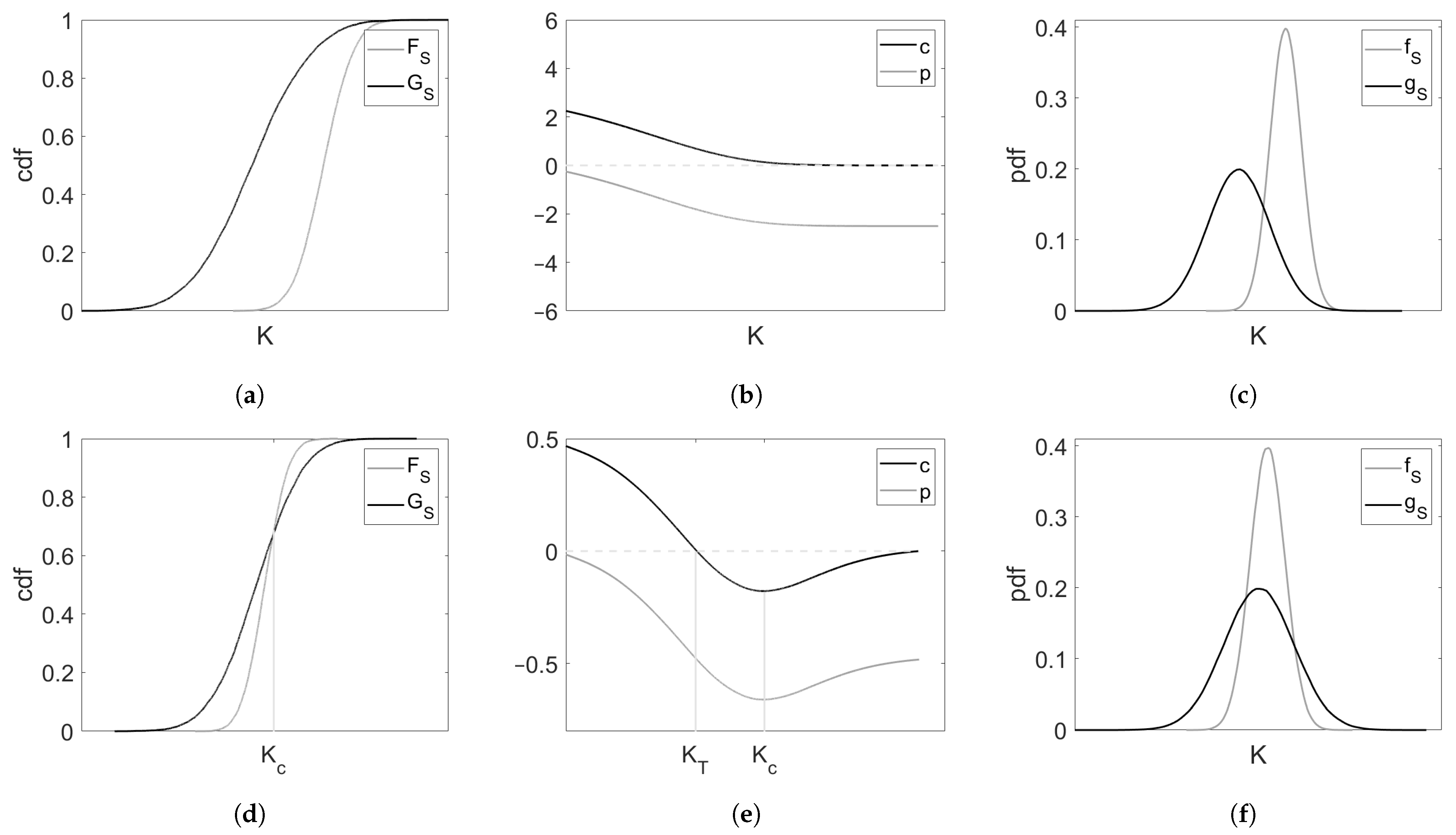
2.2. Conditions on the Existence of a Zero-Risk Premium Strike

In what follows, we discuss the conditions that guarantee a solution to Equation (6) and so the existence of a call option’s zero-risk premium strike. We also briefly touch upon the European put option case to further substantiate our focus on call options.
The zero-risk premium strike of a European call option is defined by Equation (6), which we can rewrite in terms of the asset S instead of the return R T as
K t , T + ( x K t , T ) f S ( x ) d x = K t , T + ( x K t , T ) g S ( x ) d x ,
using the T-period physical and pricing density, respectively, f S : R + R + and g S : R + R + , of asset S and the expressions in Equations (3) and (4).
As opposed to a European call option, the payoff from buying a European put ( E P ) option on asset S, at time t, is generally given by
payoff E P ( K , T ) = ( K S t + T ) + = ( K S t e R T ) + , = K S t e R T if S t e R T K 0 if S t e R T K .
The equivalent of Equation (7) for a European put option with the same features then becomes
0 K t , T ( K t , T x ) f S ( x ) d x = 0 K t , T ( K t , T x ) g S ( x ) d x .
Representing the corresponding T-period cumulative distribution functions of f S and g S as F S : R + ( 0 , 1 ) and G S : R + ( 0 , 1 ) , integration by parts of Equations (7) and (9), respectively, leads to
K t , T + ( 1 F S ( x ) ) d x = K t , T + ( 1 G S ( x ) ) d x ,
for the European call option and
0 K t , T F S ( x ) d x = 0 K t , T G S ( x ) d x ,
for the European put option. Based on Equations (10) and (11), we now define
c ( K ) = K + ( 1 F S ( x ) ) d x K + ( 1 G S ( x ) ) d x ,
p ( K ) = 0 K F S ( x ) d x 0 K G S ( x ) d x .
Typically for equity such as stocks and indices, the fundamental drift of the asset will exceed the risk-free rate of return to reflect risk compensation. Under the conditions of arbitrage-free pricing we then have
c ( 0 ) > 0 .
Using the above assumption, we present Proposition 1.
Proposition 1.
If for all x ( 0 , + ) it holds that
F S ( x ) G S ( x ) ,
there will not exist a zero-risk premium strike for the European call option on asset S, neither for the European put option on this same asset.
Proof. 
The strike K is a zero-risk premium strike for the European call option on asset S if c ( K ) = 0 . Likewise, K is a zero-risk premium strike for the European put option on asset S if p ( K ) = 0 . It is therefore sufficient to show that there exists no such strike for both functions c and p.
The expressions in Equations (12) and (13) result in, respectively, c ( ) = 0 and p ( 0 ) = 0 . Besides, it is easy to see that for each K [ 0 , + ) :
c ( K ) = F S ( K ) G S ( K ) = p ( K ) ,
and so
c ( 0 ) = p ( 0 ) = c ( ) = p ( ) = 0 .
Since c and p have the same derivative, it holds that
c ( K ) = K + c ( u ) d u = K + p ( u ) d u = p ( K ) p ( ) ,
p ( K ) = 0 K p ( u ) d u = 0 K c ( u ) d u = c ( K ) c ( 0 ) .
Now, using Equation (14), Equation (18) results in
p ( ) = c ( 0 ) < 0 .
The condition that x ( 0 , + ) : F S ( x ) G S ( x ) now easily translates in both c ( K ) 0 and p ( K ) 0 for each value of K ( 0 , + ) , using the equality in Equation (15). c 0 together with c ( 0 ) > 0 and c ( ) = 0 leads to the conclusion that c can never be zero, meaning that there exists no solution to Equation (7) and no zero-risk premium strike for the call option.
p 0 together with p ( 0 ) = 0 and p ( ) < 0 leads to the conclusion that p is always negative and so no zero-risk premium strike for the put option exists either, which ends the proof. A graphical clarification can be found in Figure 1a,b. □
First, note that the condition in Proposition 1 can be translated into F S first-order stochastically dominating G S (Denuit et al. 2005). Second, in Proposition A1, in Appendix A, we show that the positioning of the density functions as in Figure 1c, i.e., exactly one point of intersection, results in first order stochastic dominance of the respective cumulative density functions. No zero-risk premium for both the European call and European put option will exist in that situation.
Next, we derive a sufficient condition on the existence of a zero-risk premium strike for call options. In realistic circumstances, the premium to be paid for an insurance against hitting an asset level close to zero is higher than the probability of occurrence. In other words, price dominates probability in the left tail. Under this assumption, we present the following Proposition 2.
Proposition 2.
If the cumulative distribution functions F S and G S of asset S cross exactly once, meaning that there is a unique x ( 0 , + ) such that
0 < F S ( x ) = G S ( x ) < 1 ,
there exists a zero-risk premium strike for the European call option on this asset. Moreover, the zero-risk premium strike is unique. Under the same condition, there will not exist a zero-risk premium strike for the European put option on asset S.
Proof. 
Since it is assumed that price dominates probability in the left tail, it is expected for all x close to zero that
f S ( x ) g S ( x ) < 0 .
Suppose that F S and G S cross exactly once at strike K c , i.e., F S ( K c ) = G S ( K c ) . Combining the results in Equations (15) and (20), it then holds that
0 < K < K c : c ( K ) = p ( K ) = F S ( K ) G S ( K ) 0 ,
and c and p are decreasing functions for all K smaller than K c . Besides, Equation (15) results in
K > K c : c ( K ) = p ( K ) = F S ( K ) G S ( K ) 0 ,
and both c and p are increasing functions for all K larger than K c .
From Equation (12) we see that
c ( K c ) = K c + ( 1 F S ( x ) ) d x K c + ( 1 G S ( x ) ) d x , = K c + G S ( x ) F S ( x ) d x < 0 ,
and c is also negative for all K K c . As c ( ) = 0 and c only increases for K > K c , there will not exist a K [ K c , + ) such that c ( K ) = 0 . However, as c decreases over all 0 < K < K c , c ( 0 ) > 0 and c ( K c ) < 0 , there exists a unique K t , T ( 0 , K c ) such that c ( K t , T ) = 0 . This K t , T is called the zero-risk premium strike for the European call option on asset S.
As p ( 0 ) = 0 and p only decreases for all K ( 0 , K c ) , there will not exist a K in this region such that p ( K ) = 0 . Furthermore, as p only increases over all K > K c and p ( ) < 0 , there will not exist a K [ K c , + ) such that p ( K ) = 0 and thus no zero-risk premium strike for the European put option on asset S. A graphical clarification can again be found in Figure 1d,e. □
The density functions, resulting from the cumulative distribution functions in Figure 1d, are added in Figure 1f. In Proposition A2, in Appendix A, we show that the situation as presented in Figure 1f, i.e., two density functions crossing exactly twice, results in cumulative distribution functions that meet the conditions in Proposition 2. In that case, a unique zero-risk premium strike for the European call option exists.
A necessary condition for the existence of a zero-risk premium strike for European put options is that the cumulative distribution functions under the P - and Q -probability measures intersect at least twice. One can show that, in the specific situation of two intersection points, there exists at most one zero-risk premium strike for both the European call and European put option. The proof is similar to that of Proposition 2.

3. Joint Density Estimation Methodology

An accurate estimation of both the physical density and the pricing density of the underlying asset are crucial in determining the risk premium of a European call option. In what follows, we impose a U-shape on the measure change between the P - and Q -probability measures, which gives rise to the pricing strategy of Madan et al. (2020). Next, we detail how this strategy, combined with the option pricing formula of Carr and Madan (1999), results in a probability density estimate under both the P - and Q -measures.

3.1. The Pricing Density as U-Shaped Perturbation of the Physical Density

The pricing density of an asset’s return arises naturally from the corresponding physical density, acknowledging a U-shaped pricing kernel. Following Cochrane (2005), we accept the existence of a pricing kernel m ( R ) such that the price p t at time t of a security paying out a cash-flow c f ( R ) after a period of length T equals
p t = exp ( r T ) E P [ m ( R ) c f ( R ) ] ,
with r the T-period risk-free rate of return. That way, the price of a European call option at time t is represented as
price E C ( K , T ) = exp ( r T ) + ( S t e x K ) + m ( x ) f R T ( x ) d x .
The pricing kernel thus relates the price of a security to its expected payoff under measure P , i.e., it reflects a representative market player’s assessment on different states of the market: it is more valuable to earn a dollar in a state of the market where the own wealth is low (Cuesdeanu and Jackwerth 2018b).
Following Madan et al. (2020), we construct the U-shaped pricing kernel m, connecting the pricing density g to the physical density f, as the weighted sum of two exponential functions. We define
g ( x ) = C · ( 1 p ) · e η x + p · e ζ x · f ( x ) .
The constant C is needed to ensure that g is a proper density function and so
C 1 = ( 1 p ) · e η x + p · e ζ x · f ( x ) d x .
Investors’ preferences are thus characterized introducing the parameters η ( 0 , ) , ζ ( 0 , ) and p ( 0 , 1 ) . The first parameter η represents the risk aversion coefficient for being in a long position and likewise, ζ represents the risk aversion coefficient for being in a short position. The last parameter p weighs the importance of the declining part of the U-shape against the importance of the inclining part.
Note that it will be meaningful to calculate the risk premium and especially the zero-risk premium strike of a call option under the assumption of a U-shaped pricing kernel. Indeed, this kernel lifts both tails of the physical density, which results in exactly two points of intersection of the physical and corresponding pricing density. An example is given later on, in Section 4.2. Combining the results in Propositions A2 and 2, the existence and uniqueness of the zero-risk premium strike is confirmed.

3.2. The Simultaneous Calibration Procedure

The pricing of European options now enables the extraction of information on both the physical density f and the pricing density g, using the relation as introduced by Madan et al. (2020) and given in Equation (25). We determine an optimal set of parameters for the pricing model with pricing density g, by minimizing the distance between the available market prices on European options and the respective model prices. We evaluate this distance in terms of the root mean squared error (RMSE), which is defined as
RMSE = 1 N i = 1 N ( market price i model price i ) 2 ,
with N the total number of available market prices.
To calculate the model price, M o E C ( K , T ) , of a European call option, we use the pricing formula of Carr and Madan (1999):
M o E C ( K , T ) = exp ( α log ( K ) ) π 0 exp ( i ν log ( K ) ) ϱ ( ν ) d ν ,
where
ϱ ( ν ) = exp ( r T ) E Q [ exp ( i ( ν ( α + 1 ) i ) log ( S T ) ) ] α 2 + α ν 2 + i ( 2 α + 1 ) ν ,
and α a positive constant equal to 1.5. This formula makes use of the characteristic function ϕ g of the log-price process under the pricing measure Q . The numerical technique used to approximate the integral in Equation (28) is based on Fast Fourier Transforms (FFT) and Simpson’s integral weighting scheme. An extensive discussion on this technique and a derivation of the formulas in Equations (28) and (29) can be found in Madan and Schoutens (2016). Combining the model price of a European call option with the put-call parity of Stoll (1969), the price of a European put option with the same features is calculated.
The characteristic function ϕ g , defined as
ϕ g ( u ) = E Q [ exp ( i u x ) ] = + exp ( i u x ) g ( x ) d x ,
associated with the pricing density g, results from the physical characteristic function ϕ f , combining Equations (25) and (26) into
ϕ g ( u ) = ( 1 p ) · ϕ f ( u + i η ) + p · ϕ f ( u i ζ ) ( 1 p ) · ϕ f ( i η ) + p · ϕ f ( i ζ ) .
Equations (25) and (30) directly relate the pricing density g to the physical density f. We see that an optimal set of parameters for the pricing density g can be split into a set of parameters characterizing the U-shaped measure change on the one hand, and a set of parameters characterizing the physical density f on the other hand. As first reported by Madan et al. (2020), the calibration procedure thus results in a simultaneous extraction of information on both densities.

3.3. From Bilateral Gamma to Tilted Bilateral Gamma

The theory in Section 3.1 and Section 3.2 only enables the extraction of physical distributional information from option data if preceded by the allocation of a distributional family to the characteristic function ϕ f . Motivated by the results discussed in Madan et al. (2020), we similarly assume a Bilateral Gamma (BG) model for the probability density function under the physical measure.
The Bilateral Gamma model of Küchler and Tappe (2008) arises from the Variance Gamma (VG) model but encounters different speed as well as scale parameters for the Gamma distributed components. Using a mean( μ )-variance( σ 2 )-parameterization for these components, the characteristic function of the Bilateral Gamma process at time t is given by
ϕ X t B G ( x ; t ) = 1 1 i x σ p 2 μ p μ p 2 σ p 2 t 1 1 + i x σ n 2 μ n μ n 2 σ n 2 t .
Leveraging the theory in Section 3.2, we thus assume the characteristic function ϕ f equal to the one in Equation (31) of the four-parameter Bilateral Gamma family: ϕ f B G ( x ; t ) = ϕ X t B G ( x ; t ) . This assumption gives rise to the seven-parameter Tilted Bilateral Gamma (TBG) pricing model of Madan et al. (2020). According to Equation (30), the Tilted Bilateral Gamma characteristic function for the log-return x at time t, under the Q -measure is given by
ϕ g T B G ( x ; t ) = ( 1 p ) 1 1 ( i x η ) σ p 2 μ p μ p 2 σ p 2 t 1 1 + ( i x η ) σ n 2 μ n μ n 2 σ n 2 t + p 1 1 ( i x + ζ ) σ p 2 μ p μ p 2 σ p 2 t 1 1 + ( i x + ζ ) σ n 2 μ n μ n 2 σ n 2 t ( 1 p ) 1 1 i ( i η ) σ p 2 μ p μ p 2 σ p 2 t 1 1 + i ( i η ) σ n 2 μ n μ n 2 σ n 2 t + p 1 1 i ( i ζ ) σ p 2 μ p μ p 2 σ p 2 t 1 1 + i ( i ζ ) σ n 2 μ n μ n 2 σ n 2 t .
A calibration of the Tilted Bilateral Gamma model on option data results in a set of 7 optimal values for the parameters in Equation (32), from which the corresponding subset of Bilateral Gamma parameters completely determines the characteristic function in Equation (31). The translation of this information from option data into risk premia for call options, as given by Equation (5), requires an expression for the asset return density under the P - and Q -probability measures. Although a closed-form expression exists for the characteristic function under both the Bilateral Gamma and Tilted Bilateral Gamma model, we cannot find a simple expression for the physical and pricing density, respectively. However, if the characteristic function ϕ X of a univariate random variable X is integrable, the relationship between this function and the probability density function f X is given by the inverse Fourier transform
f X ( x ) = 1 2 π e i x u ϕ X ( u ) d u .
This continuous Fourier transform is approximated numerically using again Fast Fourier Transforms (FFT) and Simpson’s integral weighting scheme (Carr and Madan 1999; Madan and Schoutens 2016), which finally enables the conversion of the characteristic function into distributional information.

4. Numerical Results

The S&P500 index is used to illustrate the proposed pricing strategy and opportunities of the Tilted Bilateral Gamma model, as well as to assess the position and stability over time of the zero-risk premium strike of a one-month European call option. In comparison with this American stock index, we also use the DAX index, consisting of German constituents only. The data features of both indices are summarized in Table 1.
The option surfaces are cleaned by only using European-style out-of-the-money call and put options with a strike to spot distance smaller or equal to 30% of the spot price and a maturity between 30 and 60 days. As such, both in-the-money options and far away out-of-the-money options are eliminated to mitigate possible illiquidity concerns. Not taking into account the direction of the transaction, the mid-prices of the options are used as the market prices. We only select options with a price strictly larger than zero. The number of options available for the calibration varies from surface to surface between 780 and 1250. Interest rates are based on U.S. and German Treasury yield curves.

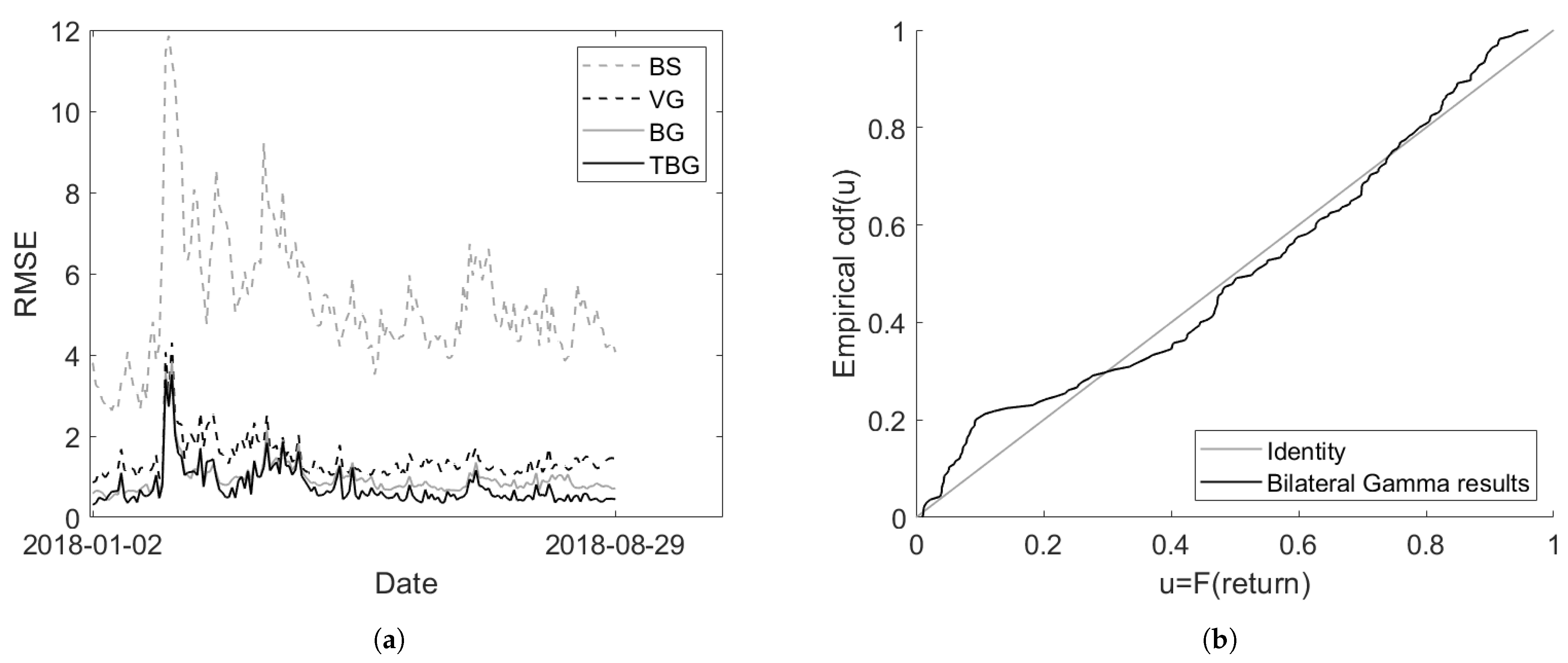
4.1. The Pricing Performance and the Quality of Physical Extraction

We first examine how well the Tilted Bilateral Gamma model is able to fit the option surface of the S&P500 index. To this purpose, we recalibrate the model on every business day for which we have option data available. Details on the resulting RMSE time series are given in Figure 2a. To compare, we add the evolution of the RMSE under the Black-Scholes (BS), Variance Gamma and Bilateral Gamma option pricing model. It is clear that the one-parameter Black-Scholes model performs poorly. The Variance Gamma model already leads to a significant improvement on the pricing performance. Extending this model to the Bilateral Gamma model results in an even better fit. In general, the Tilted Bilateral Gamma model outperforms the previous models with an average RMSE of 0.7559 over 167 calibration points, compared to an average RMSE for the other models of 5.2984, 1.4340 and 0.9625, respectively.
For a quality check of the implied Bilateral Gamma physical density we follow Madan et al. (2020), measuring the performance of the model using the probability integral transform. Let x t be the true one-month ahead return at time t of the S&P500 index. Denote by F B G the Bilateral Gamma cumulative distribution function for a monthly maturity. Define
u t = F B G ( x t , μ p , t , σ p , t , μ n , t , σ n , t ) ,
with t across the 167 estimation dates, using the optimal calibrated parameter values at each day. For a successful extraction of physical information, these data points u t should be uniformly distributed. In order to evaluate this, we graph the sorted values of u t against the cumulative distribution function of a uniformly distributed random variable. Though not perfect, a fairly promising plot is shown in Figure 2b.

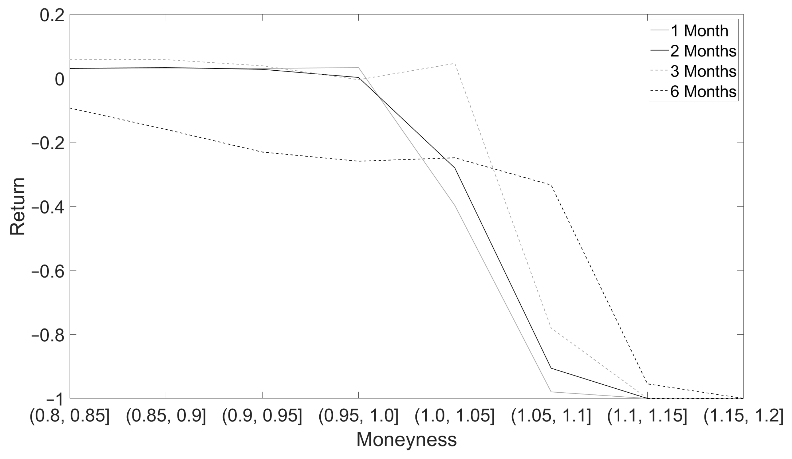
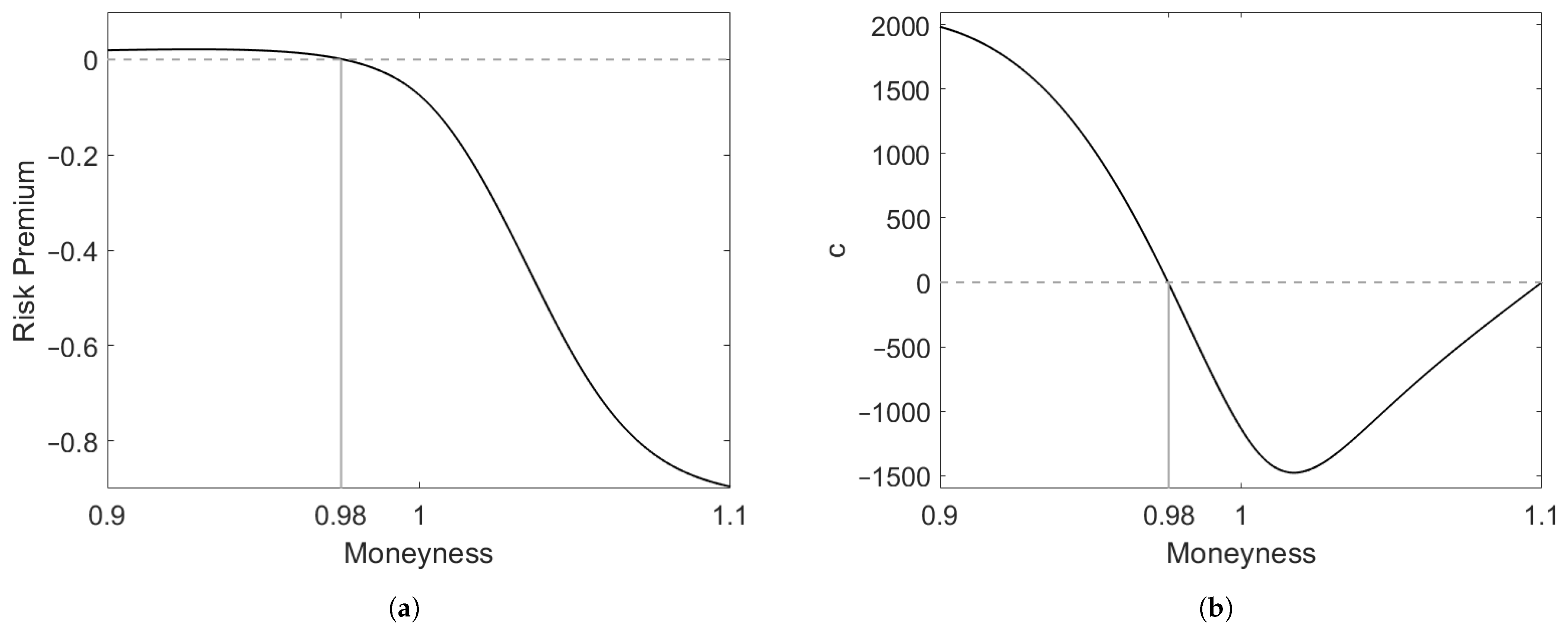
4.2. The Risk Premium of a European Call Option under the Tilted Bilateral Gamma Model

Figure 3a shows the implied physical Bilateral Gamma return density and estimated pricing Tilted Bilateral Gamma return density of the S&P500 index on 15 March 2018 (chosen arbitrarily) with a maturity equal to one month. The parameter values determining these densities are given in Table 2. To compare, we also report on the minimum, average and maximum parameter values across all calibration dates. Around the zero return, the physical density lies above the pricing density with almost no shift in the center. For large returns in absolute value, the physical density lies below the pricing density, meaning that more probability mass is carried in the tails of this pricing density.
The illustrated relative position and shape of the pricing density with respect to the physical density result from the assumption of a U-shaped pricing kernel. The calibrated, non-normalized U-shape on 15 March 2018, as set in Equation (25), is given in Figure 3b. The higher η and ζ realizations result in a more pronounced U-shape on 15 March, compared to the average shape, also shown in Figure 3b. Furthermore, investors generally assign higher prices to payoffs in negative return states, which implies more risk-aversion to large negative returns compared to large positive returns.
Next, we calculate the risk premium of European call options, with a maturity equal to one month, using again the calibration results on 15 March 2018. Moneyness is ranging from 10% in-the-money to 10% out-of-the-money. Calculating the risk premium for each moneyness level results in the graph of Figure 4a. The risk premium slightly increases to a level of 2.15%, before it starts decreasing. The zero-risk premium moneyness level k t , T amounts around 98% of the spot price, as determined by the intersection point of the curve and the zero-axis. The same shape can be found across all different calibration dates.
The average realized returns for held-to-maturity options on the S&P500 index during the sample period are presented in Figure A1, in Appendix B. We observe a similar behavior than the one in Figure 4a, for different maturities encountered.
In Figure 4b, we also show the difference in expected payoff between the P - and Q -probability measures, as defined by the function c in Equation (12). We observe the same shape than theoretically established in Proposition 2.

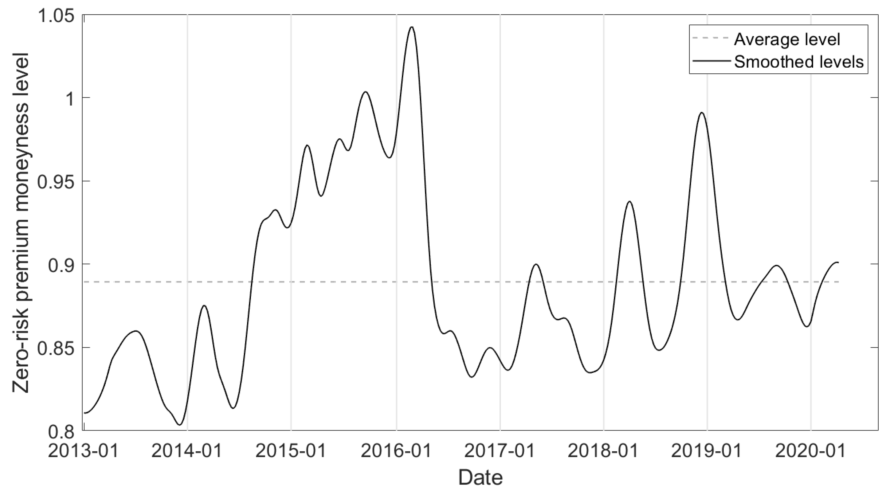
4.3. Evolution of the Zero-Risk Premium Strike

Repeating the work of Section 4.2, we assess on the evolution of the smoothed zero-risk premium strike over time, as displayed in Figure 5. We observe a minimum zero-risk premium moneyness level around 93.4%, an average zero-risk premium moneyness level around 98.5% and a maximum zero-risk premium moneyness level around 103%. The smoother highlights the fluctuations of the zero-risk premium strike around the mean level. These fluctuations are rather small in absolute value, which reveals some general stability over time.
Across the different calibration dates, we find the fairly consistent result that, within the sample period, the zero-risk premium strike of a one-month held-to-maturity European call option on the S&P500 index is located slightly in-the-money, though close to the at-the-money level. This means that only further away in-the-money call options are priced at a positive risk premium, while out-of-the-money options are expensive as resulting in a negative risk premium.
Further, the calibration procedure of Section 3.2 is also executed based on option prices with underlying the DAX index. Performing the same analysis results in the evolution of the zero-risk premium moneyness level of a one-month held-to-maturity European call option on the DAX index, as shown in Figure 6. The moneyness levels are calculated week-to-week, every Friday (see Table 1). The average zero-risk premium level amounts around 88.9%, which is lower than the average level on the S&P500 index. A minimum level around 80% is reached in the period 2013–2014, whereas a maximum level around 104% is reached at the beginning of 2016. As the analysis is performed over a longer time horizon, we clearly see some periods of lower and higher zero-risk premium strikes.

5. Conclusions

The risk premium of a European call option is defined as the relative difference in expected payoff under the P - and Q -probability measures. Historically, Coval and Shumway (2001) showed that this risk premium is increasing with moneyness, and always above the risk-free rate, under the assumption of a monotonically decreasing pricing kernel. However, this does not match with the empirically examined pattern of average realized returns on European call options. One often encounters negative returns, particularly for out-of-the-money options.
Within the framework of a U-shaped pricing kernel, we revisit risk premia in European call options and we especially focus on the option with a zero-risk premium, defined by the so-called zero-risk premium strike. We prove the uniqueness of this strike, i.e., it indicates the transition point from which on call options are considered expensive.
In order to calculate this zero-risk premium strike, pricing and physical distributional information on the return of the underlying asset is needed. While historical time series are classically used to estimate a physical distribution, we use evidence from the option market to extract information on both the physical and corresponding pricing distribution. To that purpose, we deploy the Tilted Bilateral Gamma pricing model, first introduced by Madan et al. (2020). Leveraging the distributional wealth of the option market, a calibration of this model on an option surface allows us to simultaneously extract information on both physical and pricing densities.
Based on an empirical study on the S&P500 and DAX stock index, we conclude that the zero-risk premium strike, over the covered sample period, is typically located slightly in-the-money. With small fluctuations around a mean level, the zero-risk premium strike appears to follow a rather stable pattern over time.
The research is important from a practical point of view since the joint calibration of the P - and Q -measures may lead to specific option positionings. One can trade events that are cheap in respect to the ratio of P to Q ; P reflects the likelihood of occurrence of an event in the real world, whereas Q reflects the price to be paid to bet on the realization of the corresponding event. Further, the monitoring of the zero-risk premium strike over time may be of use from a risk-management point of view as it could be informative on the market’s perception of certain risks.

Author Contributions

Writing—original draft preparation, E.V.; writing—review and editing, S.H., D.B.M. and W.S. All authors have read and agreed to the published version of the manuscript.

Funding

This research received no external funding.

Institutional Review Board Statement

Not applicable.

Informed Consent Statement

Not applicable.

Data Availability Statement

Option price data were obtained from OptionMetrics and are available at https://optionmetrics.com/ (S&P500: accessed on 31 August 2018. DAX: accessed on 17 April 2020).

Conflicts of Interest

The authors declare no conflict of interest.

Abbreviations

The following abbreviations are used in this manuscript:
BSBlack-Scholes
BGBilateral Gamma
ϕ Characteristic function
e exp
E Expected value
E C European call option
E P European put option
FFTFast Fourier Transform
fPhysical density
FPhysical cumulative probability function
gPricing density
GPricing cumulative probability function
KStrike
P Physical measure
Q Pricing measure
rRisk-free rate
RReturn on asset S
RMSERoot Mean Squared Error
SAsset
TMaturity
TBGTilted Bilateral Gamma
VGVariance Gamma

Appendix A

Proposition A1.
f and g are two probability density functions, with respective support ( a f , b f ) and ( a g , b g ) . Given is that
< a g a f < b g b f < ,
and there exists a unique c ( a g , b f ) such that
f ( x ) < g ( x ) x ( a g , c ) f ( x ) = g ( x ) 0 x = c f ( x ) > g ( x ) x ( c , b f ) .
If F and G are the cumulative distribution functions of, respectively, f and g, then F will first order stochastically dominate G, i.e., F ( x ) G ( x ) , for all x ( , + ) .
Proof. 
First of all, it is clear that for all x ( , a g ] , it holds that F ( x ) = G ( x ) = 0 , and for all x [ b f , + ) , we have F ( x ) = G ( x ) = 1 .
Second, for all x ( a g , c ] we have
F ( x ) = x f ( y ) d y < x g ( y ) d y = G ( x ) .
Now, suppose F and G intersect at least once, i.e., there exists a point x c ( a g , b f ) such that F ( x c ) = G ( x c ) . According to the result in Equation (A1), x c must be strictly larger than c. Since f and g both integrate to 1, we have
x c f ( x ) d x + x c + f ( x ) d x = x c g ( x ) d x + x c + g ( x ) d x , F ( x c ) + x c + f ( x ) d x = G ( x c ) + x c + g ( x ) d x ,
and so
x c + f ( x ) d x = x c + g ( x ) d x .
This results in
x c b g g ( x ) f ( x ) d x = b g b f f ( x ) d x .
However, since f ( x ) > g ( x ) for all x ( c , b g ) , we have a strictly negative result in the left hand side of Equation (A2) and a positive result in the right hand side. We conclude that Equation (A2) cannot be valid and F ( x ) < G ( x ) must hold for all x ( a g , b f ) . This means that F stochastically dominates G. □
Proposition A2.
f and g are two density functions, with respective support ( a f , b f ) and ( a g , b g ) . Given is that
< a g a f < b f b g < ,
and there exist exactly two points, c 1 and c 2 , such that c 1 < c 2 and
f ( x ) < g ( x ) x ( a g , c 1 ) f ( x ) = g ( x ) 0 x = c 1 f ( x ) > g ( x ) x ( c 1 , c 2 ) f ( x ) = g ( x ) 0 x = c 2 f ( x ) < g ( x ) x ( c 2 , b g ) .
If F and G are the cumulative distribution functions of, respectively, f and g, there exists a unique point x c such that 0 < F ( x c ) = G ( x c ) < 1 .
Proof. 
First, for all x ( a g , c 1 ] we have
F ( x ) = x f ( y ) d y < x g ( y ) d y = G ( x ) .
Second, for x smaller than, but close to b g , we have that f ( x ) < g ( x ) . Since g has a fatter right tail, G will reach the value of 1 slower than F and so G ( x ) < F ( x ) , for these values of x. Since G is above F when reaching values close to 0, but below F when reaching values close to 1, it is clear that F and G must intersect at least once in a point x c .
Since f ( x ) < g ( x ) for all x ( a g , c 1 ) , we have that F is flatter than G until c 1 , and so x c must be larger than c 1 . Furthermore, F is steeper than G for all x ( c 1 , c 2 ) , so F possibly intersects G in this region, but only once, at a unique point. For x larger than c 2 , F is again flatter than G, and will not cross it in this region. Since x c must exist, this means that x c ( c 1 , c 2 ) holds and this point is unique. □

Appendix B

In Figure A1, we report on the realized return of held-to-maturity call options on the S&P500 index, with varying moneyness level and maturity. The realized return is calculated as
Return = Payoff t + T Price t Price t ,
with t varying over all business days between 2 January 2018 and 29 August 2018. The given return is the average return over all values of t.
In general, we observe an overall declining behavior, for increasing moneyness, with some minor deviations for longer maturities. For the options with a one and two months maturity, the zero-risk premium strike lies around the at-the-money-level. This coincides with our findings of Section 4.3. Note that for the longer maturity of 6 months, the realized average returns are all negative for the considered moneyness range.
Figure A1. The average realized return of held-to-maturity call options on the S&P500 index, over the sample period from 2 January 2018 to 29 August 2018. 4 different maturity levels are encountered, and moneyness varies from 0.8 to 1.2.
Risks 09 00196 g0a1

Note

1
A more extensive literature focuses on the other side of the pricing kernel puzzle, i.e., on abnormal put option returns that cannot be explained by standard option models. See, e.g., Broadie et al. (2009), Bondarenko (2014) and Bernales et al. (2020). Recently, we also see some interest in the relationship between risk premia in options and volatility in the underlying asset, see Chaudhury (2017) and Hu and Jakobs (2020).

References

  1. Bakshi, Gurdip S., Dilip B. Madan, and George Panayotov. 2010. Returns of claims on the upside and the viability of U-shaped pricing kernels. Journal of Financial Economics 97: 130–54. [Google Scholar] [CrossRef]
  2. Bernales, Alejandro, Gonzalo Cortazar, Luka Salamunic, and George Skiadopoulos. 2020. Learning and Index Option Returns. Journal of Business & Economic Statistics 38: 327–39. [Google Scholar]
  3. Black, Fisher, and Myron Scholes. 1973. The pricing of options and corporate liabilities. Journal of Political Economy 18: 637–54. [Google Scholar] [CrossRef] [Green Version]
  4. Bondarenko, Oleg. 2014. Why are put options so expensive? Quarterly Journal of Finance 4: 145–95. [Google Scholar] [CrossRef]
  5. Broadie, Mark, Mikhail Chernov, and Michael S. Johannes. 2009. Understanding index option returns. The Review of Financial Studies 22: 4493–529. [Google Scholar] [CrossRef]
  6. Carr, Peter, and Dilip Madan. 1999. Option valuation using the fast Fourier transform. The Journal of Computational Finance 2: 61–73. [Google Scholar] [CrossRef] [Green Version]
  7. Chaudhury, Mo. 2017. Volatility and Expected Option Returns: A note. Economics Letters 152: 1–4. [Google Scholar] [CrossRef]
  8. Cochrane, John H. 2005. Asset Pricing, Revised ed. Princeton: Princeton University Press. [Google Scholar]
  9. Coval, Joshua D., and Tyler Shumway. 2001. Expected option returns. Journal of Finance 56: 983–1009. [Google Scholar] [CrossRef]
  10. Cuesdeanu, Horatio, and Jens C. Jackwerth. 2018a. The pricing kernel puzzle in forward looking data. Review of Derivatives Research 21: 394–419. [Google Scholar] [CrossRef] [Green Version]
  11. Cuesdeanu, Horatio, and Jens C. Jackwerth. 2018b. The pricing kernel puzzle: Survey and outlook. Annals of Finance 14: 289–329. [Google Scholar] [CrossRef] [Green Version]
  12. Denuit, Michel, Jan Dhaene, Marc Goovaerts, and Rob Kaas. 2005. Actuarial Theory for Dependent Risks: Measures, Orders and Models. West Sussex: Wiley. [Google Scholar]
  13. Harrison, Michael, and Stanley Pliska. 1981. Martingales and Stochastic Integrals in the Theory of Continuous Trading. Stochastic Processes and Their Applications 11: 215–60. [Google Scholar] [CrossRef] [Green Version]
  14. Hu, Guanglian, and Kris Jakobs. 2020. Volatility and Expected Option Returns. Journal of Financial and Quantitative Analysis 55: 1025–60. [Google Scholar] [CrossRef]
  15. Hu, Guanglian, and Yuguo Liu. 2021. The Pricing of Volatility and Jump Risks in the Cross-Section of Index Option Returns. Journal of Financial and Quantitative Analysis. forthcomming. [Google Scholar] [CrossRef]
  16. Küchler, Uwe, and Stefan Tappe. 2008. Bilateral Gamma distributions and processes in financial mathematics. Stochastic Processes and Their Applications 118: 261–83. [Google Scholar] [CrossRef] [Green Version]
  17. Madan, Dilip B., Peter P. Carr, and Eric C. Chang. 1998. The Variance Gamma process and option pricing. Review of Finance 2: 79–105. [Google Scholar] [CrossRef] [Green Version]
  18. Madan, Dilip B., and Wim Schoutens. 2016. Applied Conic Finance, 1st ed. Cambridge: Cambridge University Press. [Google Scholar]
  19. Madan, Dilip B., Wim Schoutens, and King Wang. 2020. Bilateral multiple Gamma returns: Their risks and rewards. International Journal of Financial Engineering 7: 2050008. [Google Scholar] [CrossRef]
  20. Madan, Dilip B., and Eugene Seneta. 1990. The Variance Gamma (V.G.) model for share market returns. The Journal of Business 63: 511–24. [Google Scholar] [CrossRef]
  21. McKeon, Ryan. 2019. Time Variation in Options Expected Returns. Presented at the 2019 Derivative Markets Conference; Available online: https://acfr.aut.ac.nz/__data/assets/pdf_file/0010/265339/Time-Variation-in-Option-Expected-Returns-Spring-2019.pdf (accessed on 21 October 2021).
  22. Merton, Robert C. 1973. Theory of rational option pricing. The Bell Journal of Economics and Management Science 4: 141–83. [Google Scholar] [CrossRef] [Green Version]
  23. Sichert, Tobias. 2020. The Pricing Kernel Is U-Shaped. Available online: https://papers.ssrn.com/sol3/papers.cfm?abstract_id=3095551 (accessed on 21 October 2021).
  24. Stoll, Hans R. 1969. The relationship between put and call option prices. The Journal of Finance 14: 801–24. [Google Scholar] [CrossRef]
  25. Volkmann, David. 2021. Explaining S&P500 option returns: An implied risk-adjusted approach. Central European Journal of Operations Research 29: 665–85. [Google Scholar]
Figure 1. (a) Cumulative distribution functions F S and G S of asset S under, respectively, the physical measure P and the pricing measure Q . For all x ( 0 , + ) it holds that F S ( x ) G S ( x ) . (b) Functions c and p resulting from the cumulative distribution functions in Figure 1a. (c) Density functions f S and g S resulting from the cumulative distribution functions in Figure 1a. (d) Cumulative distribution functions F S and G S under the condition that there exists exactly one x ( 0 , + ) such that F S ( x ) = G S ( x ) . (e) Functions c and p resulting from the cumulative distribution functions in Figure 1d. (f) Density functions f S and g S resulting from the cumulative distribution functions in Figure 1d. (a) F S and G S ; (b); c and p (c) f S and g S ; (d) F S and G S ; (e) c and p; (f) f S and g S .
Risks 09 00196 g001
Figure 2. (a) Evolution of the RMSE over time between optimal Black-Scholes, Variance Gamma, Bilateral Gamma and Tilted Bilateral Gamma model prices and market prices of plain-vanilla options on the S&P500 index. A calibration is conducted on each business day between 2 January 2018 and 29 August 2018. (b) Empirical, physical cumulative distribution function under the Bilateral Gamma model, evaluated at the true monthly return of the S&P500 index, in comparison with the identity function as being the cumulative distribution function of a uniform random variable. (a) Evolution RMSE; (b) Quality of BG.
Risks 09 00196 g002
Figure 3. (a) Bilateral Gamma physical density and Tilted Bilateral Gamma pricing density of the one-month ahead S&P500 index return, on 15 March 2018. (b) Calibrated U-shape of the pricing kernel on 15 March 2018 together with a time series average U-shape based on the mean parameter values across all calibration dates. (a) Pdf; (b) U-shape.
Risks 09 00196 g003
Figure 4. (a) Risk premium of the European call option with maturity equal to one month and varying moneyness levels. The underlying asset is the S&P500 index on 15 March 2018. The zero-risk premium moneyness level amounts around 98% of the spot price. (b) The difference in expected payoff under the P - and Q -probability measures, as defined by function c in Equation (12). (a) Risk Premium; (b) Difference in Expected Payoff.
Risks 09 00196 g004
Figure 5. Evolution over time of the zero-risk premium strike of a European call option on the S&P500 index, with a fixed maturity of one month. The average moneyness level amounts around 98.5%.
Risks 09 00196 g005
Figure 6. Evolution over time of the zero-risk premium strike of a European call option on the DAX index, with a fixed maturity of one month. The average moneyness level amounts around 88.9%.
Risks 09 00196 g006
Table 1. Summary of the data features of both the S&P500 and DAX index.
S&P500DAX
Option Data Source OptionMetricsOptionMetrics
Data collection 2 January 2018–29 August 20184 January 2013–3 April 2020
Frequency dailyweekly (every Friday)
Available option surfaces 167380
Currency USDEuro
Table 2. Calibrated values on 15 March 2018, for the parameters of the Tilted Bilateral Gamma model as set in Equation (32). The time series average, minimum and maximum value is also added. Average values are determined as the mean parameter values across all calibration dates.
μ p μ n σ p σ n η ζ p
15 March 20180.33870.24230.00400.005722.40307.09850.6472
Time series minimum0.16090.06870.00090.00151.00731.01900.4411
Time series average0.32040.23780.00320.008719.54956.06110.5689
Time series maximum0.81420.73820.01190.045645.519827.89610.8060
Publisher’s Note: MDPI stays neutral with regard to jurisdictional claims in published maps and institutional affiliations.

