Minimal Expected Time in Drawdown through Investment for an Insurance Diffusion Model

Abstract

Consider an insurance company whose surplus is modelled by an arithmetic Brownian motion of not necessarily positive drift. Additionally, the insurer has the possibility to invest in a stock modelled by a geometric Brownian motion independent of the surplus. Our key variable is the (absolute) drawdown $\mathsf{\Delta }$ of the surplus X, defined as the distance to its running maximum $\overline{X}$. Large, long-lasting drawdowns are unfavourable for the insurance company. We consider the stochastic optimisation problem of minimising the expected time that the drawdown is larger than a positive critical value (weighted by a discounting factor) under investment. A fixed-point argument is used to show that the value function is the unique solution to the Hamilton–Jacobi–Bellman equation related to the problem. It turns out that the optimal investment strategy is given by a piecewise monotone and continuously differentiable function of the current drawdown. Several numerical examples illustrate our findings.

1. Introduction

We model the surplus of an insurance portfolio with a diffusion approximation $X={(X_t)}_{t\ge 0}$. We assume that the insurer has the possibility of investing in an independent asset given by a Black–Scholes model $S={(S_t)}_{t\ge 0}$. That is, at time $t\ge 0$, the surplus from insurance business $X_t$ and the price of the risky asset $S_t$ are given by

$$\begin{array}{c}\hfill X_t=-x+{\mu }_{1}t+{\sigma }_1{B}_t^1,S_t={\mathrm{e}}^{\left({\mu }_2-\frac{{\sigma }_2^2}{2}\right)t+{\sigma }_2{B}_t^2},\end{array}$$

for ${\mu }_1,{\mu }_2\in \mathbb{R}$, ${\sigma }_1,{\sigma }_2>0$, and independent Brownian motions $B^1={(B_t^1)}_{t\ge 0}$, $B^2={(B_t^2)}_{t\ge 0}$. $-x\le 0$ is a constant representing the initial capital. The insurer may decide on the invested amount $A_t$ at every point in time $t\ge 0$. The surplus process $X^A={(X_t^A)}_{t\ge 0}$ under the investment strategy $A={(A_t)}_{t\ge 0}$ takes the form

$$\begin{array}{c}\hfill X_t^A=-x+{\int }_0^t({\mu }_1+A_s{\mu }_2)\mathrm{d}s+{\int }_0^t{\sigma }_1\mathrm{d}{B}_s^1+{\int }_0^t{\sigma }_2{A}_s\mathrm{d}{B}_s^2,\end{array}$$

(1)

which we can compare with (Schmidli 2008, Section 2.2.2). By ${\overline{X}}^A={({\overline{X}}_t^A)}_{t\ge 0}$, we denote the running maximum process with ${\overline{X}}_t^A=max\{0,{sup}_{s\le t}{X}_s^A\}$. The process ${\mathsf{\Delta }}^A={({\mathsf{\Delta }}_t^A)}_{t\ge 0}$ with ${\mathsf{\Delta }}_t^A={\overline{X}}_t^A-X_t^A$ is the (absolute) drawdown of $X^A$. It should be noted that these definitions allow for a positive initial offset ${\mathsf{\Delta }}_0^A=x$ of the surplus with respect to the historical maximum. The target of our analysis is to find an optimal investment strategy that minimises the expected discounted time spent with a large drawdown y

$$\begin{array}{c}\hfill v(x)=\underset{A\in \mathcal{A}}{inf}{\mathbb{E}}^x\left({\int }_0^{\infty }{\mathrm{e}}^{-\delta t}{𝟙}_{\{{\mathsf{\Delta }}_t^A>d\}}\mathrm{d}t\right).\end{array}$$

(2)

Here, $\delta >0$ and $d>0$ are preference parameters and $\mathcal{A}$ denotes the set of admissible investment strategies A, which is specified in the next section. The notation ${\mathbb{E}}^x$ is used for the expected value under the condition ${\mathsf{\Delta }}_0^A=x$, as usual. The preference parameter $\delta$ has the economic interpretation of weighing immediate drawdowns more than drawdowns in the far future. Since drawdowns imply a reduction of the surplus, this is in line with the concept of the time value of money. If a large $\delta$ is chosen, drawdowns occurring very soon have a much stronger impact on the value function than prospective drawdowns. This reflects a short-term-orientated decision-making by the insurer. On the other hand, a small discounting parameter indicates that future and current drawdowns are almost equally damaging from the insurer’s point of view. The parameter d is the critical size of drawdowns that are perceived as large and, thus, unfavourable by the insurer. That is, drawdowns exceeding d are assessed to have an adverse effect on the insurance company. The choice of this parameter would, in reality, depend on many internal and external factors, such as capital requirement, total capital, or corporate strategy. For example, if d is small in comparison to the total surplus, the value function essentially measures the time within “peaks” of the surplus process. One could think of this as the surplus being forced to grow most of the time. If d is large, the state ${\mathsf{\Delta }}_t^A>d$ can likely be associated with low values of the surplus $X^A$, so the unfavourable state of being under-capitalised for a long time is penalised. The function given in (2) is strongly related to the optimal control problem of minimising the Laplace transform of the process’ first passage through d:

$$\begin{array}{c}\hfill V(x)=\underset{A\in \mathcal{A}}{inf}{\mathbb{E}}^x\left({\mathrm{e}}^{-\delta {\tau }_A}\right),{\tau }_A:=inf\{t\ge 0:{\mathsf{\Delta }}_t^A>d\}.\end{array}$$

(3)

Since $\delta$ is positive, one could think of this as maximising the time in which the drawdown is smaller than d and the surplus has not exited the uncritical area close to the historical maximum. The difference between the two problems is that the first one will result in a strategy for an infinite time horizon, while the latter stops at the first time the drawdown is critically large. As mentioned above, our analysis shows that the problems are closely related. However, especially for long-term liabilities or if a drawdown will likely occur soon (for example, if ${\mu }_1\ll 0$), problem (2) contains more information than (3).

Drawdowns and related path functionals have attracted a lot of attention in the last 20 years. They are particularly popular in financial mathematics and economics, where they are used as a one-sided, path-dependent, and dynamic risk indicator. For instance, the “conditional drawdown at risk” is considered by Chekhlov et al. (2005) in the context of portfolio optimisation. Another more recent example is found in (Maier-Paape and Zhu 2018), where a risk measure depending on the proportional drawdown (which measures the percentage loss) is constructed. In addition to measuring risks, drawdowns and maximum drawdowns have also been linked to market crashes (compare (Sornette 2003) and (Zhang and Hadjiliadis 2012)) and have been used to quantify performance (Hamelink and Hoesli 2004).

Much research has been conducted on drawdowns of actuarial and financial models as probabilistic objects as well. Distributional properties of the drawdowns of standard and arithmetic Brownian motions were investigated by Douady et al. (2000), Graversen and Shiryaev (2000), and Salminen and Vallois (2007). Other articles deal with first passage times, such as ${\tau }_A$ defined in (3). An example covering a broad scope is due to Mijatović and Pistorius (2012), who studied the joint distribution of the first passage time and related quantities for spectrally negative Lévy processes. Another example containing results specifically for one-dimensional diffusions is (Zhang 2015). In (Landriault et al. 2015), the frequency of drawdowns larger than a critical level is examined for an arithmetic Brownian motion. In (Landriault et al. 2017), the magnitude of the drawdown and the so-called “time to recover” are considered. The term “time to recover” refers to the duration until the historical running maximum is re-reached, which is related to our problem for small values of d. Wang et al. (2020) analysed a Gerber–Shiu-type expected penalty function for the drawdown, extending the classical results of Gerber and Shiu (1998).

A popular approach in the field of stochastic optimisation aims to minimise ruin probabilities, severity of ruin, or functionals thereof (see, for example, (Browne 1995)). However, ruin is a rare and extreme event, which is why ruin-related quantities merely serve as a conceptual measure of risk. In reality, it is more likely that an economic unit will aim to enhance its capital or to prevent diminishment. This motivates the consideration of optimisation problems related to drawdowns. In the context of portfolio selection, Grossman and Zhou (1993) introduced a utility maximisation problem under “drawdown constraints”. This means that one admits only those portfolios that prevent large drawdowns of the wealth process. Their results were extended by Cvitanic and Karatzas (1995), Elie and Touzi (2008), and Cherny and Obloj (2013). Another possibility is to put drawdowns into the focus of the optimisation and introduce drawdown-based value functions. A prominent example is the minimisation of the probability that a large (proportional) drawdown occurs. Chen et al. (2015) consider this problem for an investment model. Angoshtari, Bayraktar, and Young published a series of papers dealing with the optimisation of drawdown probabilities under investment and consumption (compare Angoshtari et al. (2015, 2016a, 2016b)). Han et al. (2018, 2019) examined problems connected to the minimisation of the probability of a drawdown under proportional reinsurance.

However, the above literature does not take into account the length of a drawdown. Intuitively, it is clear that a drawdown has, in general, a negative connotation. Even if the business is profitable, frequent drawdowns can affect the value of a company negatively through an indirect psychological impact on managers, policyholders, shareholders, and potential partners. The following simple example illustrates the situation. Imagine that the surplus of the company under consideration increases from 100 to 130 EUR and then drops by 28 EUR. Despite the positive profit, one cannot help feeling a disappointment about the relative loss. Similar psychological effects have been observed in the context of decreasing dividend payments (compare (Albrecher et al. 2018)). An additional factor playing an influential role is the duration of a drawdown. If the surplus recovers shortly after the drawdown, inattentive policyholders might not notice the changes. However, a long-lasting drawdown can be interpreted as a consequence of flawed business decisions or general managerial inefficiency. The present manuscript contributes to the existing research by analysing the optimal control problems (2) and (3), which reflect both aspects, the severity and the duration of a drawdown. Differently from (Brinker and Schmidli 2020), we allow the possibility of investment. With this in mind, the following results can be seen as a first step towards understanding optimal investment decisions based on multiple drawdown key indicators.

The rest of this paper is organised as follows. In the next section, we specify the model we are working with. With Section 3, the main part of this paper is devoted to solving the optimal control problem (3). We use a fixed-point argument to show that the Hamilton–Jacobi–Bellman equation (HJB equation) associated with the problem has a unique solution. We identify this solution as the value function (3) and conclude that the optimal strategy is a monotone function of the current drawdown. Neither the value function nor the optimal investment strategy can explicitly be calculated, but fixed-point iteration allows us to calculate both in numerical examples. In the last section, we use these results to solve the original problem given in (2). Our ansatz is the natural extension to the strategy maximising the time until a large drawdown occurs: Under the assumption that the initial drawdown exceeds d, we find the strategy minimising the time with large drawdown. In principle, one could repeat the steps of Section 3 with slight modifications to prove existence of a solution to the connected HJB equation. However, in this case, we explicitly obtain the solution using a different approach. The key argument is that the drawdown process behaves like a diffusion without reflection above the critical level d. The optimal strategy turns out to be constant such that well-known results on passage times of arithmetic Brownian motions apply. We connect the return functions of the two subproblems and verify that their composition is the solution to our original problem (2). We draw conclusions from our results and give numerical examples for the expected discounted time spent in drawdown.

2. The Model and Its Parameters

Throughout the paper, we work on a complete probability space $(\mathsf{\Omega },\mathcal{F},\mathbb{P})$ equipped with the natural filtration ${({\mathcal{F}}_t)}_{t\ge 0}$ generated by the two-dimensional Brownian motion $(B^1,B^2)$. We assume that the investment strategies are càdlàg and adapted with values in the bounded interval $[\underline{a},\overline{a}](\ni 0)$. It will turn out that this restriction of the maximally invested amount is necessary for the problem to be well defined. The inclusion of zero in this interval means that it is possible not to invest. Moreover, we assume that either ${\mu }_1\ge 0$, or if ${\mu }_1<0$, then there exists $a\in [\underline{a},\overline{a}]$ with ${\mu }_1+{\mu }_{2}a\ge 0$. This means that either the insurance portfolio is expected to be profitable or that it is possible to invest in such a way that is expected to generate profits. The reason we include the case ${\mu }_1<0$ is that insurance premiums are calculated in advance, and if adjustments are contractually permitted, they are usually tied to certain key dates or other conditions. That means that, particularly for long-term liabilities, it is possible that unexpectedly severe or frequent claims occur in contract portfolios or divisions. Even though insurers evaluate risks regarding their profitability before issuing contracts, there are prominent examples, such as life insurance policies with high guaranteed fixed interest rates or the insurance of flood risk, which have turned out to be non-profitable. In this case, drawdown-minimising strategies might be used to prevent or shorten “negative tours” from the previous level.

In order to define the set of admissible strategies $\mathcal{A}$, we first observe that the controlled drawdown process and running maximum together form a solution to the Skorohod problem for $-X^A$ (compare, for example, (Pilipenko 2014)). That is, the pair $(Y,L)=({\mathsf{\Delta }}^A,{\overline{X}}^A)$ solves

• $Y_t\ge 0$ for all $t\ge 0$,
• L is non-decreasing with $L_0=0$,
• ${\int }_0^t{𝟙}_{\{Y_s>0\}}\mathrm{d}{L}_s=0$ for all $t\ge 0$,
• Almost surely for all $t\ge 0$:

  $$Y_t=x+L_t-{\int }_0^t{\mu }_1+A_s{\mu }_2\mathrm{d}s-{\int }_0^t{\sigma }_1\mathrm{d}{B}_s^1-{\int }_0^t{\sigma }_2{A}_s\mathrm{d}{B}_s^2.$$

  (4)

One important implication of the third condition is that whenever L increases, Y must be equal to zero. If a solution $(Y,L)$ to the reflected equation (4) is known, the surplus process $X^A$ is given by $X^A=L-Y$. In case the strategy A is of feedback form $A_t=a({\mathsf{\Delta }}_t^A)$ depending on the current drawdown through a function $a:[0,\infty )\to \mathbb{R}$, (4) is a reflected stochastic differential equation. Hence, we define $\mathcal{A}$ as the set of strategies A, which are càdlàg and adapted processes with values in the interval $[\underline{a},\overline{a}]$, such that a solution to (4) exists and is unique. It is clear that the process under the strategy $A_t=0$, $t\ge 0$, exists and we will use this strategy of “doing nothing” as a reference in our numerical examples. Concerning the “well-posedness” of the problem (2) for all parameter sets, it is important that the discounting factor $\delta$ is strictly positive. Otherwise, the integral might not exist if the drawdown process spends infinite time above the level d. For example, if ${\mu }_1<0$, ${\mathsf{\Delta }}_t$ tends to infinity as $t\to \infty$ almost surely and the indicator function will ultimately be equal to one. So, in this case, the value of the strategy of never investing is not finite. On the other hand, as the indicator function is at most equal to one, the return of all strategies is bounded from above by ${\delta }^{-1}$. This implies that (2) is well posed for every $\delta >0$. The value function V of the optimal control problem (3) is bounded from above by 1.

3. Maximising the Time to Drawdown

Assume that initially, the surplus process is uncritically close to the running maximum, meaning that ${\mathsf{\Delta }}_0^A=x\in [0,d]$. Intuitively, and since immediate drawdowns have a larger weight than future drawdowns, the optimal strategy is to maximise the time ${\tau }_A:=inf\{t\ge 0:{\mathsf{\Delta }}_t^A>d\}$ in the uncritical area. In fact, one can reason this intuition with a dynamic programming principle, as was done in (Brinker and Schmidli 2020) for the optimisation of reinsurance. Hence, we consider the following auxiliary problem. We let the function $V(x)$ be defined as in (3) for $x\in [0,d]$. This is the Laplace transform of the first time the drawdown process hits d, and it clearly becomes minimal when ${\tau }_A$ is maximised. The boundary condition $V(d)=1$ has to be fulfilled. By the theory of stochastic control, this problem is connected to the HJB equation:

$$\begin{array}{c}\hfill -\delta V(x)-{\mu }_1{V}^{\prime }(x)+\frac{{\sigma }_1^2}{2}{V}^{″}(x)+\underset{a\in [\underline{a},\overline{a}]}{inf}-{\mu }_{2}a{V}^{\prime }(x)+\frac{{\sigma }_2^2{a}^2}{2}{V}^{″}(x)=0.\end{array}$$

(5)

We start with some heuristics on the function V. If the initial drawdown is $x>y$ with $x,y\in [0,d]$, there are two possible scenarios. If the drawdown process arrives at y before exiting the interval $[0,d]$, it will then spend the same time in the favourable area as a process of initial drawdown y. However, it is also possible that the drawdown overshoots the critical level d before reaching y. In this case, the process leaves the favourable area earlier. Now, intuitively, this means that the time the process spends in $[0,d]$ should be smaller when the initial drawdown is larger. Comparing small values x and y, we expect that y is reached quickly and that it is almost impossible for the drawdown to exceed d before. On the other hand, if x and y are close to the boundary d, it is easier for the paths to “slip” out of the interval, so in this case, the effect should be stronger. In other words, we presume that V is an increasing and convex function. At this point, this is just an educated guess, since our heuristics neither took the preference factor $\delta$ into account, nor the time passing until y is visited for the first time. We prove at end of this section that, in fact, V has those properties. In order to see which other characteristics we are looking for, we start with a verification theorem.

Theorem 1.

Let $f:[0,d]\to [0,1]$ be a twice continuously differentiable, non-decreasing function with $f^{\prime }(0)=0$. Moreover, assume that f solves (5) with pointwise optimiser $a:[0,d]\to [\underline{a},\overline{a}]$. Then, $f=V$, and the strategy $A^{\ast }\in \mathcal{A}$ with $A_t^{\ast }=(a({\mathsf{\Delta }}_t^{A^{\ast }}))$, $t\ge 0$, is optimal.

Proof. 

By Itô’s formula, we have for an arbitrary strategy $A\in \mathcal{A}$:

$$\begin{array}{cc}\hfill & {\mathrm{e}}^{-\delta (t\wedge {\tau }_A)}f({\mathsf{\Delta }}_{t\wedge {\tau }_A}^A)-f({\mathsf{\Delta }}_0^A)\hfill \\ & ={\int }_0^{t\wedge {\tau }_A}{\mathrm{e}}^{-\delta s}{f}^{\prime }({\mathsf{\Delta }}_s^A)\mathrm{d}{\overline{X}}_s^A-{\int }_0^{t\wedge {\tau }_A}{\sigma }_1{\mathrm{e}}^{-\delta s}{f}^{\prime }({\mathsf{\Delta }}_s^A)\mathrm{d}{B}_s^1-{\int }_0^{t\wedge {\tau }_A}{\sigma }_2{A}_s{\mathrm{e}}^{-\delta s}{f}^{\prime }({\mathsf{\Delta }}_s^A)\mathrm{d}{B}_s^2\hfill \\ \hfill & +{\int }_0^{t\wedge {\tau }_A}{\mathrm{e}}^{-\delta s}\left[-\delta f({\mathsf{\Delta }}_s^A)-({\mu }_1+{\mu }_2{A}_s)f^{\prime }({\mathsf{\Delta }}_s^A)+\left(\frac{{\sigma }_1^2}{2}+\frac{{\sigma }_2^2{A}_s^2}{2}\right)f^{″}({\mathsf{\Delta }}_s^A)\right]\mathrm{d}s.\hfill \end{array}$$

Now, since the running maximum only increases at times where the drawdown is zero and $f^{\prime }(0)=0$, the first integral is equal to zero. By continuity (and hence boundedness over compacts) of the derivative of f, the two stochastic integrals are martingales. The last integral is non-negative. Thus, taking expectations, we find

$$\begin{array}{c}\hfill {\mathbb{E}}^x\left({\mathrm{e}}^{-\delta (t\wedge {\tau }_A)}f({\mathsf{\Delta }}_{t\wedge {\tau }_A}^A)\right)\ge f(x).\end{array}$$

By the boundedness of f, we can take the limit $t\to \infty$ to find $V^A(x)\ge f(x)$. Taking the infimum over the set $\mathcal{A}$ of admissible strategies, we conclude $V(x)\ge f(x)$. As we will see below, it follows from the HJB equation that $A^{\ast }$ is an admissible strategy. Thus, repeating the above argumentation for the strategy $A^{\ast }$, we see that f is the value of this strategy and that $V=f$. □

Example 1

(${\mu }_2=0$). If ${\mu }_2=0$, investing in the second active only results in an increased volatility without any expected steady income. Therefore, we expect that it is never optimal to buy units of the risky asset in this case. The HJB equation becomes particularly simple under this assumption:

$$\begin{array}{c}\hfill -\delta V(x)-{\mu }_1{V}^{\prime }(x)+\frac{{\sigma }_1^2}{2}{V}^{″}(x)=0,V(d)=1,V^{\prime }(0)=0.\end{array}$$

Solving this ordinary differential equation, we find

$$\begin{array}{cc}\hfill f(x)& =\frac{q_1{\mathrm{e}}^{q_{2}x}-q_2{\mathrm{e}}^{q_{1}x}}{q_1{\mathrm{e}}^{q_{2}d}-q_2{\mathrm{e}}^{q_{1}d}},q_1=\frac{{\mu }_1+\sqrt{{\mu }_1^2+2\delta {\sigma }_1^2}}{{\sigma }_1^2},q_2=\frac{{\mu }_1-\sqrt{{\mu }_1^2+2\delta {\sigma }_1^2}}{{\sigma }_1^2},\hfill \end{array}$$

as a candidate solution. A quick calculation shows that this function is increasing and strictly convex, such that ${\sigma }_2^2{a}^2/2·f^{″}(x)$ becomes minimal at $a=0$. f solves (5) and $V=f$ is verified by Theorem 1.

In the following, we consider the more complicated case ${\mu }_2\ne 0$. We focus on the case ${\mu }_2>0$, where holding the risky asset leads to expected profits. The case ${\mu }_2<0$ (where short selling leads to expected profits) can be treated analogously. This is because we could consider the Brownian motion ${\tilde{B}}^2=-B^2$, the positive drift component ${\tilde{\mu }}_2=-{\mu }_2$, and the strategy $\tilde{A}=-A$ to transform the problem: An optimal strategy for the model with ${\mu }_2<0$ can be obtained by mirroring an optimal strategy for the case of positive drift around the x-axis. In view of Theorem 1, our ansatz is to show the existence of a solution to the HJB equation on the interval $[0,d]$.

3.1. Construction of a Solution to (5)

Throughout this subsection, we assume that ${\mu }_2>0$ holds. We denote by $\mathcal{C}[x_1,x_2]$ the space of continuous functions that are defined on the closed interval $[x_1,x_2]$ endowed with the supremum norm $\parallel ·\parallel$. We roughly follow the approach in (Belkina et al. 2014) by defining an operator, the fixed point of which is a solution to the HJB equation. This idea works for the presented problem, even though the results in (Belkina et al. 2014) apply to the classical risk model under a different value function. Assume that V is, in fact, an increasing solution to the HJB equation and that we know the optimiser $a(x)$ at a certain point x. Then, rearranging the terms of the HJB equation, we have

$$V^{″}(x)=2\frac{\delta \left(V(0)+{\int }_0^x{V}^{\prime }(y)\mathrm{d}y\right)+({\mu }_1+{\mu }_{2}a(x))V^{\prime }(x)}{{\sigma }_1^2+{\sigma }_2^{2}a{(x)}^2}.$$

For any other $a\in [\underline{a},\overline{a}]$, the equation holds with “≥” in place of “=”. This inspires the definition of the operator $\mathsf{L}$ with

$$\begin{array}{c}\hfill \mathsf{L}u(x)=2\underset{a\in [\underline{a},\overline{a}]}{sup}\frac{\delta \left(\mathsf{\Lambda }+{\int }_0^{x}u(y)\mathrm{d}y\right)+({\mu }_1+{\mu }_{2}a)u(x)}{{\sigma }_1^2+{\sigma }_2^2{a}^2}\end{array}$$

(6)

for all functions $u\in \mathcal{C}[0,d]$. $\mathsf{\Lambda }\in \mathbb{R}$ represents the unknown value $V(0)$. Since the value $V(d)=1$ is known, it might seem counter-intuitive not to write $V(x)=1-{\int }_x^{d}V(y)\mathrm{d}y$. In the following, we will see that the above is more useful. We observe that for every $u\in \mathcal{C}[0,d]$, $\mathsf{L}u$ is finite for every $x\in [0,d]$. We will now show that for every $\mathsf{\Lambda }$, there exists a unique $u\in \mathcal{C}[0,d]$, such that $u^{\prime }(x)=\mathsf{L}u(x)$ holds with initial condition $u(0)=0$. We use a fixed-point argument, so our first step is to construct a contraction. As a preparation, we need the following Lemmas.

Lemma 1.

For $ϵ>0$, we define the function ${\varphi }_{ϵ}:\mathbb{R}\to [0,\infty )$ by

$$\begin{array}{c}\hfill {\varphi }_{ϵ}(a)=\frac{2\delta ϵ+|{\mu }_1+{\mu }_{2}a|}{{\sigma }_1^2+a^2{\sigma }_2^2}.\end{array}$$

${\varphi }_{ϵ}$ attains a global maximum. As $ϵ\to 0$, $ϵ{\varphi }_{ϵ}(a)$ converges to zero uniformly in a. In particular, there exists $ϵ>0$ such that $ϵ{\varphi }_{ϵ}(m)<1$, where m denotes the global maximum of ${\varphi }_{ϵ}$.

Proof. 

Let

$$\begin{array}{cc}\hfill a_1& =-\frac{(2\delta ϵ+{\mu }_1){\sigma }_2-\sqrt{{(2\delta ϵ+{\mu }_1)}^2{\sigma }_2^2+{\sigma }_1^2{\mu }_2^2}}{{\mu }_2{\sigma }_2},a_2=\frac{(2\delta ϵ-{\mu }_1){\sigma }_2-\sqrt{{(2\delta ϵ-{\mu }_1)}^2{\sigma }_2^2+{\sigma }_1^2{\mu }_2^2}}{{\mu }_2{\sigma }_2}.\hfill \end{array}$$

A direct calculation shows that ${\varphi }_{ϵ}$ attains its global maximum at m, where

$$\begin{array}{c}\hfill m=\left\{\begin{array}{cc}{a}_1>0,\hfill & \mathrm{if} {\mu }_1\ge 0,{\mu }_2>0,\hfill \\ a_2<0,\hfill & \mathrm{if} {\mu }_1<0,{\mu }_2>0.\hfill \end{array}\right.\end{array}$$

Both $a_i$ converge as $ϵ\to 0$. Hence, ${\varphi }_{ϵ}(m)$ converges and $ϵ{\varphi }_{ϵ}(m)\to 0$ for $ϵ\to 0$. □

The first part of Lemma 1 is used to define the Lipschitz constant in the next result.

Lemma 2.

For an arbitrary $\mathsf{\Lambda }\in \mathbb{R}$, $\eta \in [0,d)$, and $ϵ\in (0,d-\eta ]$, we define $\mathsf{T}:\mathcal{C}[\eta ,\eta +ϵ]\to \mathcal{C}[\eta ,\eta +ϵ]$ through

$$\begin{array}{c}\hfill \mathsf{T}u(x)=2\underset{a\in [\underline{a},\overline{a}]}{sup}\frac{\delta \left(\mathsf{\Lambda }+{\int }_{\eta }^{x}u(y)\mathrm{d}y\right)+({\mu }_1+{\mu }_{2}a)u(x)}{{\sigma }_1^2+{\sigma }_2^2{a}^2}\end{array}$$

for $x\in [\eta ,\eta +ϵ]$. Let ${\varphi }_{ϵ}$ and m be defined as in Lemma 1. The operator $\mathsf{T}$ fulfils

$$\begin{array}{c}\hfill \parallel \mathsf{T}u-\mathsf{T}w\parallel \le {\varphi }_{ϵ}(m)\parallel u-w\parallel ,\end{array}$$

for all $u,v\in \mathcal{C}[\eta ,\eta +ϵ]$, so it is Lipschitz-continuous with respect to the uniform norm on $[\eta ,\eta +ϵ]$.

Proof. 

For all $a\in [\underline{a},\overline{a}]$, we define

$$\begin{array}{c}\hfill {\mathsf{T}}^{a}u(x)=2\frac{\delta \left(\mathsf{\Lambda }+{\int }_{\eta }^{x}u(y)\mathrm{d}y\right)+({\mu }_1+{\mu }_{2}a)u(x)}{{\sigma }_1^2+{\sigma }_2^2{a}^2}.\end{array}$$

Now, $x\mapsto {\mathsf{T}}^{a}u(x)$ is continuous for all $u\in \mathcal{C}[\eta ,\eta +ϵ]$ and, hence, uniformly continuous on the compact set $[\eta ,\eta +ϵ]$. Thus, the maximum $x\mapsto \mathsf{T}u(x)$ of the uniformly continuous functions is continuous as well. Next, we show that all operators ${\mathsf{T}}^a$ are Lipschitz-continuous with a common constant. Let $u,w\in \mathcal{C}[\eta ,\eta +ϵ]$. We have

$$\begin{array}{cc}\hfill & \parallel {\mathsf{T}}^{a}u-{\mathsf{T}}^{a}w\parallel \hfill \\ \hfill & \le \frac{2}{{\sigma }_1^2+a^2{\sigma }_2^2}\left(\delta \underset{x\in [\eta ,\eta +ϵ]}{sup}{\int }_{\eta }^x|u(y)-w(y)|\mathrm{d}y+|{\mu }_1+{\mu }_{2}a|\underset{x\in [\eta ,\eta +ϵ]}{sup}|u(x)-w(x)|\right)\hfill \\ \hfill & \le \frac{2\delta ϵ+|{\mu }_1+{\mu }_{2}a|}{{\sigma }_1^2+a^2{\sigma }_2^2}\parallel u-w\parallel ={\varphi }_{ϵ}(a)\parallel u-w\parallel .\hfill \end{array}$$

Since ${\varphi }_{ϵ}(a)$ becomes maximal at m, we have found ${\varphi }_{ϵ}(m)$ as common Lipschitz-constant. This bound is not necessarily sharp, since we only consider a from the bounded interval $[\underline{a},\overline{a}]$. Now, we show the Lipschitz-continuity of $\mathsf{T}$. We consider again $u,w\in \mathcal{C}[\eta ,\eta +ϵ]$. We fix $x\in [\eta ,\eta +ϵ]$ and assume that $\mathsf{T}u(x)\ge \mathsf{T}w(x)$. By definition of $\mathsf{T}$ and ${\mathsf{T}}^a$, for every $\widetilde{ϵ}>0$, there is some $a(x)\in [\underline{a},\overline{a}]$, such that $|\mathsf{T}u(x)-{\mathsf{T}}^{a(x)}u(x)|<\widetilde{ϵ}$. We have $\mathsf{T}w(x)\ge {\mathsf{T}}^{a(x)}w(x)$ and, hence,

$$\begin{array}{cc}\hfill |\mathsf{T}u(x)-\mathsf{T}w(x)|& \le |\mathsf{T}u(x)-{\mathsf{T}}^{a(x)}u(x)|+{\mathsf{T}}^{a(x)}u(x)-{\mathsf{T}}^{a(x)}w(x)\hfill \\ \hfill & \le \widetilde{ϵ}+|{\mathsf{T}}^{a(x)}u(x)-{\mathsf{T}}^{a(x)}w(x)|\le \widetilde{ϵ}+{\varphi }_{ϵ}(m)\parallel u-w\parallel .\hfill \end{array}$$

Similarly, we could have derived the same upper bound in the case $\mathsf{T}u(x)\le \mathsf{T}w(x)$. The left-hand side does not depend on $\widetilde{ϵ}$, such that we can let $\widetilde{ϵ}\searrow 0$. Hence, we have

$$\begin{array}{c}\hfill |\mathsf{T}u(x)-\mathsf{T}w(x)|\le {\varphi }_{ϵ}(m)\parallel u-w\parallel \end{array}$$

for every $x\in [\eta ,\eta +ϵ]$. We can now take the supremum on the left-hand side to conclude that $\mathsf{T}$ is Lipschitz-continuous with respect to the uniform norm. □

Remark 1.

Lemma 2 implies that $\mathsf{L}$ maps $\mathcal{C}[0,d]$ onto itself and is Lipschitz-continuous with respect to the uniform norm on $[0,d]$ when $\eta =0$, $ϵ=d$.

Now, we use the second part of Lemma 1 for defining a contraction.

Lemma 3.

Let ϵ be chosen sufficiently small, such that $ϵ{\varphi }_{ϵ}(m)<1$. Let $\mathsf{T}$ be defined as in Lemma 2 and let λ be given. The map $\mathsf{J}:\mathcal{C}[\eta ,\eta +ϵ]\to \mathcal{C}[\eta ,\eta +ϵ]$ with

$$\begin{array}{c}\hfill \mathsf{J}w(x)=\lambda +{\int }_{\eta }^x\mathsf{T}w(y)\mathrm{d}y,w\in \mathcal{C}[\eta ,\eta +ϵ],\end{array}$$

is a contraction, and thus has a unique fixed point u. u is continuously differentiable on $(\eta ,\eta +ϵ)$ with $u(\eta )=\lambda$. Moreover, $u^{\prime }(x)=\mathsf{T}u(x)$.

Proof. 

$\mathsf{J}$ is a well-defined map from a complete space to itself. To conclude that it is also a contraction, we take $u,w\in \mathcal{C}[\eta ,\eta +ϵ]$ and observe:

$$\begin{array}{c}\hfill \parallel \mathsf{J}u-\mathsf{J}w\parallel \le |x-\eta |{\varphi }_{ϵ}(m)\parallel u-w\parallel \le ϵ{\varphi }_{ϵ}(m)\parallel u-w\parallel <\parallel u-w\parallel .\end{array}$$

The properties of the fixed point follow from the definitions of $\mathsf{J}$ and $\mathsf{T}$, respectively. □

Now, we compose the solutions on the subintervals to construct a function on $[0,d]$.

Lemma 4.

For every Λ, there exists a unique continuously differentiable function $u\in \mathcal{C}[0,d]$, such that $u^{\prime }=\mathsf{L}u$ and $u(0)=0$.

Proof. 

We divide the interval $[0,d]$ into N parts, choosing a large enough N such that $ϵ=d{N}^{-1}$ fulfils $ϵ{\varphi }_{ϵ}(m)<1$. We define the operators

$$\begin{array}{cc}\hfill {\mathsf{T}}^{(0)}w(x)& =2\underset{a\in [\underline{a},\overline{a}]}{sup}\frac{\delta \left(\mathsf{\Lambda }+{\int }_0^{x}w(y)\mathrm{d}y\right)+({\mu }_1+{\mu }_{2}a)w(x)}{{\sigma }_1^2+{\sigma }_2^2{a}^2},\hfill \\ \hfill {\mathsf{J}}^{(0)}w(x)& ={\int }_0^x{\mathsf{T}}^{(0)}w(y)\mathrm{d}y,\hfill \end{array}$$

for $w\in \mathcal{C}[0,d{N}^{-1}]$, and by Lemma 3, the latter has the unique fixed point $u^{(0)}$ with $u^{(0)}(0)=0$ and continuous derivative ${\mathsf{T}}^{(0)}{u}^{(0)}$. Now, we let

$$\begin{array}{c}\hfill {\mathsf{\Lambda }}_0={\int }_0^{d{N}^{-1}}{u}^{(0)}(y)\mathrm{d}y,{\lambda }_0=u^{(0)}(d{N}^{-1}).\end{array}$$

Inductively, we define on $\mathcal{C}[kd{N}^{-1},(k+1)d{N}^{-1}]$

$$\begin{array}{cc}\hfill {\mathsf{T}}^{(k)}w(x)& =2\underset{a\in [\underline{a},\overline{a}]}{sup}\frac{\delta \left({\mathsf{\Lambda }}_{k-1}+{\int }_{kd{N}^{-1}}^{x}w(y)\mathrm{d}y\right)+({\mu }_1+{\mu }_{2}a)w(x)}{{\sigma }_1^2+{\sigma }_2^2{a}^2},\hfill \\ \hfill {\mathsf{J}}^{(k)}w(x)& ={\lambda }_{k-1}+{\int }_{kd{N}^{-1}}^x{\mathsf{T}}^{(k)}w(y)\mathrm{d}y\hfill \end{array}$$

and

$$\begin{array}{c}\hfill {\mathsf{\Lambda }}_k=\sum _{j=0}^k{\int }_{jd{N}^{-1}}^{(j+1)d{N}^{-1}}{u}^{(j)}(y)\mathrm{d}y,{\lambda }_k=u^{(k)}((k+1)d{N}^{-1})\end{array}$$

for $k=1,\dots ,N-1$, where $u^{(k)}$ denotes the unique fixed point of ${\mathsf{J}}^{(k)}$. From the definition of the sequence $({\lambda }_k)$, we conclude that the composition

$$\begin{array}{c}\hfill u(x)=u^{(0)}(x)·{\mathbb{I}}_{[0,d{N}^{-1}]}(x)+\sum _{k=1}^{N-1}{u}^{(k)}(x)·{\mathbb{I}}_{(kd{N}^{-1},(k+1)d{N}^{-1}]}(x)\end{array}$$

is continuous. From the definition of the sequence $({\mathsf{\Lambda }}_k)$, we get that the derivative is also continuous and given by

$$\begin{array}{c}\hfill u^{\prime }(x)=2\underset{a\in [\underline{a},\overline{a}]}{sup}\frac{\delta \left(\mathsf{\Lambda }+{\int }_0^{x}u(y)\mathrm{d}y\right)+({\mu }_1+{\mu }_{2}a)u(x)}{{\sigma }_1^2+{\sigma }_2^2{a}^2}.\end{array}$$

If $\tilde{u}$ is a $\mathcal{C}[0,d]$-function with ${\tilde{u}}^{\prime }=\mathsf{L}\tilde{u}$ and $\tilde{u}(0)=0$, then it is continuously differentiable, and $\tilde{u}{|}_{[0,d{N}^{-1}]}$ is a fixed point of $J^{(0)}$. Because this functional is a contraction, $\tilde{u}{|}_{[0,d{N}^{-1}]}=u^{(0)}$. Repeating this argument for all subintervals $[k,(k+1)d{N}^{-1}]$, we find $\tilde{u}=u$. □

We reverse our hypothetical calculations for V to show that the anti-derivative of the constructed function solves the HJB equation.

Theorem 2.

Let u be defined as in Lemma 4. The anti-derivative $U(x)=\mathsf{\Lambda }+{\int }_0^{x}u(y)\mathrm{d}y$ is twice continuously differentiable. It holds that $U(0)=\mathsf{\Lambda }$ and $U^{\prime }(0)=0$. The function is the unique solution to $U^{″}(x)=\mathsf{L}{U}^{\prime }(x)$ and the HJB equation with these initial conditions.

Proof. 

Differentiability, initial values and uniqueness are a direct consequence from the definition of U and Lemma 4. Let $a(x)\in [\underline{a},\overline{a}]$ denote the maximiser of $\mathsf{L}{U}^{\prime }(x)$. We have

$$\begin{array}{c}\hfill U^{″}(x)=2\frac{\delta U(x)+({\mu }_1+{\mu }_{2}a(x))U^{\prime }(x)}{{\sigma }_1^2+{\sigma }_2^{2}a{(x)}^2},\end{array}$$

(7)

which is equivalent to

$$\begin{array}{c}\hfill -\delta U(x)-{\mu }_1{U}^{\prime }(x)+\frac{{\sigma }_1^2}{2}{U}^{″}(x)-{\mu }_{2}a(x)U^{\prime }(x)+\frac{{\sigma }_2^2{\left[a(x)\right]}^2}{2}{U}^{″}(x)=0.\end{array}$$

Since (7) holds with “≥” in place of “=” for all $a\in [\underline{a},\overline{a}]$, U solves the HJB equation. In the same way as in the beginning of this subsection, we obtain that every solution $\tilde{U}$ to the HJB equation matching the initial conditions is a solution to ${\tilde{U}}^{″}(x)=\mathsf{L}{\tilde{U}}^{\prime }(x)$. This implies uniqueness for the HJB equation. □

In the next two Lemmas, we derive properties of the function U and the optimiser a on the condition that the initial value $\mathsf{\Lambda }$ is positive.

Lemma 5.

Let U be defined as in Theorem 2 for $\mathsf{\Lambda }>0$. For all $x>0$, it holds that $U^{\prime }(x)>0$ and U is strictly convex. The optimiser $a(x)$ is continuous and non-negative with $a(0)=0$ and $a(x)=\alpha (x)\wedge \overline{a}$, where

$$\begin{array}{cc}\hfill \alpha (x)& :=\frac{{\mu }_2{U}^{\prime }(x)}{{\sigma }_2^2{U}^{″}(x)}.\hfill \end{array}$$

(8)

$\alpha (x)$ is continuously differentiable. If, additionally, ${\mu }_1\ge 0$, then $U^{″}$ is strictly increasing.

Proof. 

We have by $U^{\prime }(0)=0$:

$$\begin{array}{c}\hfill U^{″}(0)=\mathsf{L}{U}^{\prime }(0)=2\underset{a\in [\underline{a},\overline{a}]}{sup}\frac{\delta \mathsf{\Lambda }}{{\sigma }_1^2+{\sigma }_2^2{a}^2}=\frac{2\delta \mathsf{\Lambda }}{{\sigma }_1^2}>0,\end{array}$$

(9)

so $a(0)=0$ and $\alpha (0)=0$. By the continuity of $U^{″}$, it follows that $U^{\prime }(x)$ is strictly increasing, at least in a small environment $x\in [0,x_0)$, $x_0>0$. On $(0,x_0]$, it holds that $U^{\prime }(x)>0$. If we define $y_0:=inf\{x\ge x_0:U^{\prime }(x)<0\}$, we have $U^{\prime }(y_0)=0$ by continuity. Again, as in (9), $U^{″}(y_0)>0$. This is not possible because $y_0$ is defined as the first time that $U^{\prime }(x)$ enters the negative half plane, meaning that it must be decreasing at this time. Hence, $U^{\prime }(x)>0$ for $x>0$. Now, suppose that there was $z_0$ such that $U^{″}(z_0)=0$. Then,

$$\begin{array}{c}\hfill \delta U(z_0)+({\mu }_1+{\mu }_{2}a)U^{\prime }(z_0)\le 0\end{array}$$

for all $a\in [\underline{a},\overline{a}]$. This is a contradiction: The first term must be positive and the second term is non-negative, at least for $\overline{a}$, by assumption. We conclude: $U^{″}(x)>0$ for all $x\ge 0$. It follows directly that the optimiser is non-negative:

$$\begin{array}{c}\hfill 0<U^{″}(x)=2\underset{a\in [0,\overline{a}]}{sup}\frac{\delta U(x)+({\mu }_1+{\mu }_{2}a)U^{\prime }(x)}{{\sigma }_1^2+{\sigma }_2^2{a}^2}.\end{array}$$

(10)

All variables inducing a negative counter are already excluded, and all values of $a<0$ with a positive counter are dominated by the value at $a=0$. Moreover, since U solves the HJB equation and is increasing and convex, the optimiser takes the form $a(x)=\alpha (x)\wedge \overline{a}$. Continuity of $\alpha$ implies continuity of a.

Deriving the right-hand side of (10) with respect to a shows that the maximum is attained at

$$\begin{array}{c}\hfill \alpha (x)=\frac{-[\delta U(x)+{\mu }_1{U}^{\prime }(x)]+\sqrt{{[\delta U(x)+{\mu }_1{U}^{\prime }(x)]}^2{\sigma }_2^2+{\mu }_2^2{\sigma }_1^2{\left[U^{\prime }(x)\right]}^2}}{{\sigma }_2{\mu }_2{U}^{\prime }(x)},\end{array}$$

(11)

or on the boundary $\overline{a}$. From this representation of $\alpha$ in terms of U and $U^{\prime }$, it follows that $\alpha$ is continuously differentiable.

Now, we show that the second derivative increases in the special case. If ${\mu }_1\ge 0$, it holds that

$$\begin{array}{c}\hfill \delta U(x)+({\mu }_1+{\mu }_{2}a)U^{\prime }(x)<\delta U(z)+({\mu }_1+{\mu }_{2}a)U^{\prime }(z)\end{array}$$

(12)

for every $a\in [0,\overline{a}]$ if $x<z$. By (10), this implies that $U^{″}(x)<U^{″}(z)$ and $U^{″}$ is strictly increasing. □

Lemma 6.

We assume that the conditions of Lemma 5 hold and define

$$\begin{array}{c}\hfill {\overline{a}}_0=\frac{-{\mu }_1{\mu }_2+\sqrt{{({\mu }_1{\mu }_2)}^2+2\delta {\mu }_2^2{\sigma }_1^2}}{2\delta {\sigma }_2^2}>0.\end{array}$$

1. 

If $\overline{a}\ge {\overline{a}}_0$, it holds that $a(x)=\alpha (x)$ and a is strictly increasing up to the point where it reaches ${\overline{a}}_0$, and is constant from there on. $a(x)$ is continuously differentiable on $(0,d)$ with existing limits ${lim}_{h\downarrow 0}{a}^{\prime }(h)$ and ${lim}_{h\uparrow d}{a}^{\prime }(h)$.

2. 

If $\overline{a}<{\overline{a}}_0$, there exists $x_0:=inf\{x>0:\alpha (x)=\overline{a}\}$. It holds that $a(x)=\alpha (x)$ for $x\le x_0$ and $a(x)=\overline{a}$ for $x\ge x_0$. $a(x)$ is continuously differentiable on $(0,x_0\wedge d)$ and on $(x_0\wedge d,x_0\vee d)$ with existing limits ${lim}_{h\downarrow 0}{a}^{\prime }(h)$, ${lim}_{x\uparrow x_0}{a}^{\prime }(x)$, ${lim}_{x\downarrow x_0}{a}^{\prime }(x)$, and ${lim}_{h\uparrow d}{a}^{\prime }(h)$.

Proof. 

Since $\overline{a}>0$ and $a(0)=0$, we have $a(x)=\alpha (x)$ for sufficiently small x by Lemma 5. We let $x_0=inf\{x>0:a(x)=\overline{a}\wedge {\overline{a}}_0\}>0$. In particular, by $\overline{a},{\overline{a}}_0>0$ and $a(0)=0$, we have $a(x)=\alpha (x)$ for all $x\le x_0$. We firstly show that $\alpha$ is increasing at least in a small environment of zero. We have $U^{\prime }(0)=0$ and $U(0),U^{″}(0)>0$, so there exists $ϵ>0$ such that

$$\begin{array}{c}\hfill U^{\prime }{(x)}^2-U(x)U^{″}(x)<0\end{array}$$

(13)

for all $x\in (0,ϵ)$. This means that $x\mapsto \frac{U(x)}{U^{\prime }(x)}$ is strictly decreasing on this interval. Hence,

$$\begin{array}{c}\hfill x\mapsto 2\frac{\delta \frac{U(x)}{U^{\prime }(x)}+({\mu }_1+{\mu }_{2}a)}{{\sigma }_1^2+{\sigma }_2^2{a}^2}\end{array}$$

is decreasing in x for every a, meaning that $x\mapsto \frac{U^{″}(x)}{U^{\prime }(x)}$ is decreasing. However, then, $\alpha (x)=\frac{{\mu }_2}{{\sigma }_2^2}\frac{U^{\prime }(x)}{U^{″}(x)}$ is increasing for $x\in [0,ϵ)$.

Now, either (13) holds for all $x\le x_0$ and $\alpha (x)=a(x)$ is strictly increasing up to $x_0$, or there exists at least one point $x\in [ϵ,x_0]$ with $U^{\prime }{(x)}^2-U(x)U^{″}(x)=0$. We write $z_0=sup\{x>0:U^{\prime }{(x)}^2-U(x)U^{″}(x)<0\}$. Then, $\alpha (x)=a(x)$ is strictly increasing up to $z_0$. Using that $U(z_0)/U^{\prime }(z_0)=U^{\prime }(z_0)/U^{″}(z_0)$, we conclude from the HJB equation that

$$\begin{array}{c}\hfill (2\delta {\sigma }_2^2+{\mu }_2^2)\alpha {(z_0)}^2+2{\mu }_1{\mu }_2\alpha (z_0)-\frac{{\mu }_2^2{\sigma }_1^2}{{\sigma }_2^2}=0.\end{array}$$

So, by the non-negativity of the optimiser, $\alpha (z_0)=a(z_0)={\overline{a}}_0$. This is a contradiction in the case $\overline{a}<{\overline{a}}_0$, so $a(x)=\alpha (x)$ is strictly increasing on $[0,x_0)$ with $x_0=inf\{x>0:\alpha (x)=\overline{a}\}$. If $\overline{a}\ge {\overline{a}}_0$, we get that $a(x)=\alpha (x)$ is strictly increasing on $[0,x_0)$ with $x_0=inf\{x>0:\alpha (x)={\overline{a}}_0\}=z_0$.

In the case $\overline{a}<{\overline{a}}_0$, the optimiser $a(x)=\overline{a}$ is constant for $x\ge x_0$. This is shown via direct calculation using the ansatz $U(x)=U(x_0)(c_1{\mathrm{e}}^{q_1(\overline{a})(x-x_0)}+c_2{\mathrm{e}}^{q_2(\overline{a})(x-x_0)})$, where the constants fulfil $c_1+c_2=1$ and $\frac{{\mu }_2}{{\sigma }_2^2}\frac{U^{\prime }(x_0)}{U^{″}(x_0)}=\overline{a}$. In the second case of $\overline{a}>{\overline{a}}_0$, it holds that $U(x)=U(z_0){\mathrm{e}}^{{\mu }_2{\sigma }_2^{-2}{\overline{a}}_0(x-z_0)}$ with constant optimiser $a(x)={\overline{a}}_0=\alpha (x)$ for $x\ge z_0$, if $z_0$ exists. This means that the optimiser is strictly increasing on $[0,z_0)$. Once it reaches ${\overline{a}}_0$, it is “trapped” there and constant for all $x>z_0$.

By $a(x)=\alpha (x)$, it follows that a is continuously differentiable on $(0,d)$ if $\overline{a}\ge {\overline{a}}_0$. The limit ${lim}_{h\uparrow d}{a}^{\prime }(h)$ exists because $\alpha$ is strictly increasing, continuous, and bounded from above. To show that ${lim}_{h\downarrow 0}{a}^{\prime }(h)$ is finite, we make the following observation. Since a is differentiable and the denominator of (7) is positive, the third derivative of U exists and is continuous on $(0,d)$. This means that the derivative of a takes the form $a^{\prime }(x)=\frac{U^{\prime }(x)U^{‴}(x)-{(U^{″}(x))}^2}{{(U^{″}(x))}^2}$. Suppose that ${lim}_{h\downarrow 0}{a}^{\prime }(h)=+\infty$. Then, it must hold that ${lim}_{h\downarrow 0}{U}^{‴}(h)=+\infty$ because U is strictly convex. However, on the other hand, it holds that

$$\begin{array}{c}\hfill \left(\frac{{\sigma }_1^2}{2}+\frac{{\mu }_2^2{(U^{\prime }(x))}^2}{2{\sigma }_2^2{(U^{″}(x))}^2}\right)U^{‴}(x)=\delta U(x)-{\mu }_1{U}^{″}(x)-\frac{{\mu }_2}{{\sigma }_2^2}{U}^{\prime }(x),\end{array}$$

which follows from differentiating the HJB equation after plugging in the optimiser $\alpha (x)$. Now, if we let $x\to 0$, the bracket term on the left-hand side converges to a positive value. The right-hand side also converges, which contradicts the unboundedness of the third derivative. Hence, ${lim}_{h\uparrow d}{a}^{\prime }(h)<\infty$. If $\overline{a}<{\overline{a}}_0$, a is continuously differentiable on $(0,x_0\wedge d)$ and on $(x_0\wedge d,d)$. If the latter interval is non-empty, the derivative is equal to zero. Existence of the limits ${lim}_{h\downarrow 0}{a}^{\prime }(h)$, ${lim}_{x\uparrow x_0}{a}^{\prime }(x)$ follows in the same way as in the case $\overline{a}\ge {\overline{a}}_0$. □

Remark 2.

1. 

This Lemma implies that U calculated with $a\in [0,{\overline{a}}_0]$ also solves the HJB equation for the unbounded case where the strategy may be chosen from the interval $(-\infty ,\infty )$.

2. 

We note that throughout the considerations above, $d>0$ was arbitrary. The uniqueness implies that if $d_0>d$ and $U^0$ is the solution defined on $[0,d_0]$, then $U=U^0{|}_{[0,d]}$. Moreover, the optimiser a does not depend on d.

Now, we relate the constructed solution to the value function V and an optimal strategy.

3.2. Solution to the Optimisation Problem

In view of Theorem 1, our natural candidate for the value function is the solution to the HJB equation, which is equal to one at $x=d$. Thus, for $\mathsf{\Lambda }=1$ and $U(x)=1+{\int }_0^{x}u(y)\mathrm{d}y$ defined as in Theorem 2, we let

$$\begin{array}{c}\hfill f(x)=\frac{U(x)}{U(d)},x\in [0,d].\end{array}$$

(14)

Theorem 3.

If ${\mu }_2>0$, f defined in (14) is the unique solution to the HJB equation (5) with $f(d)=1$ and $f^{\prime }(0)=0$. f is strictly increasing except at zero, and is strictly convex. The pointwise optimiser $a(x)$ has the properties stated in Lemmas 5 and 6. Moreover, $V(x)=f(x)$ for all $x\in [0,d]$, and the strategy $A^{\ast }\in \mathcal{A}$ with $A_t^{\ast }=(a({\mathsf{\Delta }}_t^{A^{\ast }}))$, $t\ge 0$, is optimal.

Proof. 

The properties of f follow by Lemma 5. We observe that f solves the HJB equation under the initial conditions $f(0)={(U(d))}^{-1}$ and $f^{\prime }(0)=0$, as it is a positive multiple of the solution U. The optimiser remains the same. Since $a(x)$ is continuously differentiable, except possibly at one point $x_0>0$, and the derivative is bounded for $x\to 0$, it is Lipschitz-continuous on $[0,d]$. This implies that (4) has a unique strong solution (compare, for example, (Pilipenko 2014), Theorem 2.1.1). The verification of f being the value function and $A^{\ast }$ being optimal follow from Theorem 1. □

Thus, we have shown that V is strictly increasing except at zero, and is strictly convex. The optimal strategy is the feedback strategy defined in Theorem 1 with optimiser $a(x)$. The function a fulfils $a(0)=0$ and is strictly increasing until either $\overline{a}$ or ${\overline{a}}_0$ is reached. This means that if the drawdown is small, nothing is invested, and as the drawdown approaches the critical line, slightly more is invested. This holds true for the case ${\mu }_2>0$. Analogously, we could have shown:

Theorem 4.

If ${\mu }_2<0$, V is the unique solution to the HJB equation (5) with $V(d)=1$ and $V^{\prime }(0)=0$. V is strictly increasing except at zero, and is strictly convex. The pointwise optimiser $a(x)=\frac{{\mu }_2{V}^{\prime }(x)}{{\sigma }_2^2{V}^{″}(x)}\vee \underline{a}$ fulfils $a(0)=0$ and is continuously differentiable except possibly at one positive point. It is strictly decreasing until it is constant and bounded from below by

$$\begin{array}{c}\hfill {\underline{a}}_0=\frac{-{\mu }_1{\mu }_2-\sqrt{{({\mu }_1{\mu }_2)}^2+2\delta {\mu }_2^2{\sigma }_1^2}}{2\delta {\sigma }_2^2}<0.\end{array}$$

In the next subsection, we consider some numerical examples.

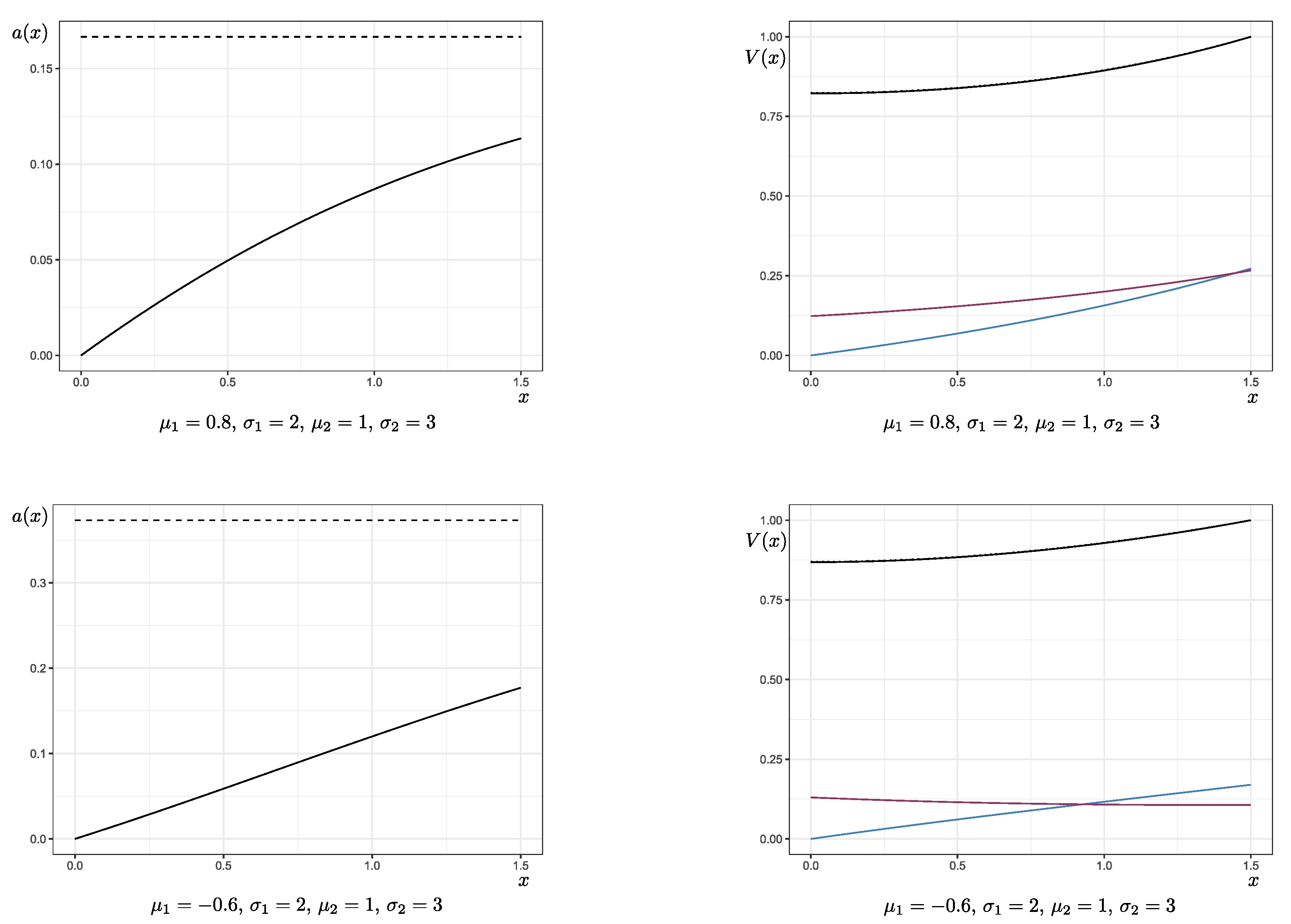
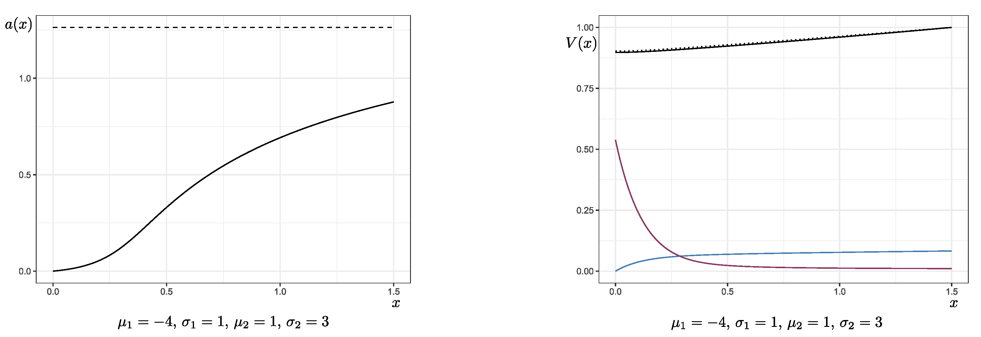
3.3. Numerical Examples

We assume that the technical discounting factor is $\delta =0.3$. The relatively small $\delta$ reflects a long-term strategy, as this would be preferable, for example, in the context of life insurance. We define $d=1.5$ as the critical size in these numerical examples. However, as noted in Remark 2, the choice of d does not affect the shape of the function $a(x)$. Figure 1 shows the optimal strategy inducing function $a(x)$ and Laplace transform $V(x)$ of the first passage through d for different combinations of ${\mu }_1$, ${\sigma }_1$, ${\mu }_2$, and ${\sigma }_2$. In the graphs of the first row, the income from the insurance business is already expected to be profitable (${\mu }_1=0.8$, ${\sigma }_1=2$). The goal of the insurer is to elongate the time until the first significant drawdown occurs via investment in a risky asset, which yields a higher return at the cost of increased uncertainty (${\mu }_2=1$, ${\sigma }_2=3$). In comparison, the second row displays the functions in the same situation, but for the case where the insurance portfolio consists of non-profitable contracts (${\mu }_1=-0.6$). The graphs in the third row belong to an example of extremely negative drift, ${\mu }_1=-4$, ${\sigma }_1=1$, ${\mu }_2=1$, and ${\sigma }_2=3$, which is mainly included to show the variation in shape of the function $a(x)$. In all cases, it holds that ${\mu }_2>0$ and $\overline{a}>{\overline{a}}_0$, and the solutions were obtained via fixed-point iteration.

According to Lemma 6, the function $a(x)$ is strictly increasing with $a(0)=0$ and bounded from above by the constant ${\overline{a}}_0$. If the drawdown approaches the critical value d, the amount invested increases up to the level ${\overline{a}}_0$. The drift from the investment is supposed to keep the process’ paths in the uncritical area. ${\overline{a}}_0$ is the critical value for which the added volatility from the investment is too risky and may push the process over the critical line. In the numerical examples, it can be observed that, if the drift of the original portfolio ${\mu }_1$ is negative, the investment function $a(x)$ grows larger in a shorter time. If, for regulatory reasons, it held that ${\overline{a}}_0>\overline{a}$, the function a would retain its shape, except for staying at $\overline{a}$ once this level is reached (see Section 4.1 for an example with $\overline{a}<{\overline{a}}_0$). As shown in Theorem 3 the value function is increasing and convex in all cases. Moreover, only in the case of ${\mu }_1=0.8\ge 0$, the second derivative of V is increasing as well. For a comparison, the Laplace transform of the first passage through d under the strategy of never investing, that is, $A_t=0$ for all $t\ge 0$, is pictured in the graphs on the right-hand side (dotted lines). We see here that V is only slightly smaller. However, this effect will be striking for the solution of the general problem.

4. Minimising the Expected Time with Large Drawdown

Since we have already found the optimal strategy that maximises the time with a small drawdown, it is natural to extend this with the strategy that minimises the time with a large drawdown: $W(x)={sup}_{A\in \mathcal{A}}{\mathbb{E}}^x({\mathrm{e}}^{-\delta {\tau }^A})$ for ${\tau }^A:=inf\{t\ge 0:{\mathsf{\Delta }}_t^A<d\}$. We start by considering constant strategies. As it turns out, this is sufficient for the case of a large initial drawdown.

Since the drawdown process under the constant strategy a behaves like an arithmetic Brownian motion of drift $-({\mu }_1+{\mu }_{2}a)$ and variance ${\sigma }_1^2+{\sigma }_2^2{a}^2$ as long as it is above d, the value $W^a$ of this strategy inherits its structure from the Laplace transform of the hitting time of a Brownian motion:

Lemma 7.

For $a\in [\underline{a},\overline{a}]$ define ${\varphi }_a(q)=\frac{{\sigma }_1^2+{\sigma }_2^2{a}^2}{2}{q}^2-({\mu }_1+{\mu }_{2}a)q$ and

$$\begin{array}{c}\hfill q_2(a)=\frac{({\mu }_1+{\mu }_{2}a)-\sqrt{{({\mu }_1+{\mu }_{2}a)}^2+2\delta ({\sigma }_1^2+{\sigma }_2{a}^2)}}{{\sigma }_1^2+{\sigma }_2{a}^2}.\end{array}$$

$q_2(a)$ is the negative solution to ${\varphi }_a(q)=\delta$. The value of the strategy A, which is constant and equal to a, is given by $W^a(x)={\mathrm{e}}^{q_2(a)(x-d)}$ for all $x\ge d$.

Theorem 5.

If ${\mu }_2\ge 0$ holds in combination with $|\underline{a}|\le \overline{a}$ or with $|\underline{a}|>\overline{a}$ and $\delta \le {\varphi }_{\overline{a}}(\frac{2{\mu }_2}{{\sigma }_2^2(\overline{a}+\underline{a})})$, the best constant strategy is $A=\overline{a}$. Otherwise, $A=\underline{a}$ is the best constant strategy. If ${\mu }_2<0$ holds in combination with $|\underline{a}|\ge \overline{a}$ or with $|\underline{a}|<\overline{a}$ and $\delta \le {\varphi }_{\overline{a}}(\frac{2{\mu }_2}{{\sigma }_2^2(\overline{a}+\underline{a})})$, the best constant strategy is $A=\underline{a}$. Otherwise, $A=\overline{a}$ is the best constant strategy. Let $\check{a}$ denote the respective optimiser. It holds that $W=W^{\check{a}}$ for $x\ge d$ and $A=\check{a}$ is optimal.

Proof. 

We conclude from the previous Lemma that we have to maximise $q_2(a)$. Since $q_2(a)$ itself is hard to handle as a function of a, we consider the functions ${\varphi }_a$ instead. For every a, ${\varphi }_a^{″}(x)={\sigma }_1^2+{\sigma }_2^2{a}^2>0$, so the function is strictly decreasing up to its first zero. It holds that ${\varphi }_a(0)=0$, so there can be at most one negative solution to ${\varphi }_a(q)=\delta$. We start with the case ${\mu }_2\ge 0$. For all a with $\left|a\right|<\overline{a}$, it holds that

$$\begin{array}{c}\hfill \frac{{\varphi }_{\overline{a}}(q)-{\varphi }_a(q)}{\overline{a}-a}=\frac{{\sigma }_2^2{q}^2(\overline{a}+a)}{2}-{\mu }_{2}q>0\end{array}$$

for all $q<0$. For $\left|a\right|=\overline{a}$ with $a<0$, ${\varphi }_{\overline{a}}(q)-{\varphi }_a(q)=-{\mu }_{2}q(\overline{a}-a)\ge 0$. In either case, it holds that ${\varphi }_{\overline{a}}(q)\ge {\varphi }_a(q)$, which implies that $q_2(\overline{a})\ge q_2(a)$.

Now, we assume $|\underline{a}|>\overline{a}$. Let $a\in (\underline{a},-\overline{a})$. Similarly as before, we have ${\varphi }_{\overline{a}}(q)-{\varphi }_a(q)\ge 0$ for all $q\in [\frac{2{\mu }_2}{{\sigma }_2^2(\overline{a}+a)},0)$. On the other hand, ${\varphi }_{\underline{a}}(q)-{\varphi }_a(q)\ge 0$ for all $q\in (-\infty ,\frac{2{\mu }_2}{{\sigma }_2^2(\underline{a}+a)}]$. By $0>\overline{a}+a>\underline{a}+a$, we conclude that ${\varphi }_a(q)$ lies below ${\varphi }_{\overline{a}}(q)$ or ${\varphi }_{\underline{a}}(q)$ for all $q<0$, and thus cannot induce the maximum. We still have to compare the values on the boundary if $|\underline{a}|>\overline{a}$. It holds that ${\varphi }_{\overline{a}}(q)-{\varphi }_{\underline{a}}(q)\ge 0$ iff $q\in [\frac{2{\mu }_2}{{\sigma }_2^2(\overline{a}+\underline{a})},0)$. This means that the optimiser is $\overline{a}$, in case ${\varphi }_{\overline{a}}(\frac{2{\mu }_2}{{\sigma }_2^2(\overline{a}+\underline{a})})={\varphi }_{\underline{a}}(\frac{2{\mu }_2}{{\sigma }_2^2(\overline{a}+\underline{a})})\ge \delta$. The case ${\mu }_2<0$ follows analogously.

Now, let $\check{a}$ denote the optimiser in the respective cases. We conclude that for every a, it holds that $-\delta -{\varphi }_a(q_2(\check{a}))\le 0$ with equality in the case $a=\check{a}$. Thus, $W^{\check{a}}$ solves

$$\begin{array}{c}\hfill -\delta W(x)-{\mu }_1{W}^{\prime }(x)+\frac{{\sigma }_1^2}{2}{W}^{″}(x)+\underset{a\in [\underline{a},\overline{a}]}{sup}-{\mu }_{2}a{W}^{\prime }(x)+\frac{{\sigma }_2^2{a}^2}{2}{W}^{″}(x)=0,\end{array}$$

(15)

for $x\ge d$. The assertion is verified in the same way as in the proof of Theorem 1. □

Now, to solve our original problem, we connect the solutions to the two subproblems. Our ansatz for the optimal strategy is $A^{\ast }$ with

$$\begin{array}{c}\hfill A_t^{\ast }=\left\{\begin{array}{cc}a({\mathsf{\Delta }}_t^{A^{\ast }}),\hfill & \mathrm{if} {\mathsf{\Delta }}_t^{A^{\ast }}\le d,\hfill \\ \check{a},\hfill & \mathrm{if} {\mathsf{\Delta }}_t^{A^{\ast }}>d,\hfill \end{array}\right.\end{array}$$

(16)

for $t\ge 0$. In the case that this is continuous, the existence of the controlled surplus process follows as in the proof of Theorem 3. Otherwise, weak existence of the controlled drawdown follows by Theorem 4.1 of (Rozkosz and Slominski 1997). In the non-degenerate case of ${\mu }_2\ne 0$, a construction similar to the one in Theorem 4.2 of (Semrau 2009) ensures pathwise uniqueness (choose $h(x)=-2({\mu }_1+{\mu }_{2}a(x))/({\sigma }_1^2+{\sigma }_2^{2}a{(x)}^2)$, $\phi (x)={\int }_0^x{\mathrm{e}}^{h(y)}\mathrm{d}y$, and use that ${\phi }^{\prime }$ is bounded away from zero). The Yamada–Watanabe-type Theorem 333 of (Situ 2005) therefore implies strong existence and uniqueness.

Theorem 6.

Let $V:[0,d]\to [0,{\delta }^{-1}]$ denote the maximal time to drawdown from the previous section and let $W:[d,\infty )\to [0,{\delta }^{-1}]$ denote the minimal time in drawdown. We define

$$\begin{array}{c}\hfill f(x)=\left\{\begin{array}{cc}\frac{-q_2(\check{a})V(x)}{\delta (V^{\prime }(d)-q_2(\check{a}))},\hfill & if x\le d,\hfill \\ \frac{1}{\delta }-\left(\frac{1}{\delta }-\frac{-q_2(\check{a})}{\delta (V^{\prime }(d)-q_2(\check{a}))}\right)W(x),\hfill & if x>d.\hfill \end{array}\right.\end{array}$$

It holds that $v=f$ and $A^{\ast }$, defined as in (16), is an optimal strategy.

Proof. 

We have already seen that f solves (5) on $[0,d]$ with $f^{\prime }(0)=0$, where the second derivative is assumed to be one-sided for $x\in \{0,d\}$. Equation (15) implies that this differential equation can be extended on $[d,\infty )$ in the sense that f solves

$$\begin{array}{c}\hfill -\delta f(x)-{\mu }_1{f}^{\prime }(x)+\frac{{\sigma }_1^2}{2}{f}^{″}(x)+\underset{a\in [\underline{a},\overline{a}]}{inf}-{\mu }_{2}a{f}^{\prime }(x)+\frac{{\sigma }_2^2{a}^2}{2}{f}^{″}(x)=-{𝟙}_{x>d}.\end{array}$$

(17)

f can be written as the difference of two convex functions (with a bounded derivative), so by Theorem 4.3 in (Björk 2015), it follows that

$$\begin{array}{cc}\hfill & ({\mathrm{e}}^{-\delta t}f({\mathsf{\Delta }}_t^A)-f({\mathsf{\Delta }}_0^A)\hfill \\ \hfill & -{\int }_0^t{\mathrm{e}}^{-\delta s}\left[-\delta f({\mathsf{\Delta }}_s^A)-({\mu }_1+{\mu }_2{A}_s)f^{\prime }({\mathsf{\Delta }}_s^A)+\left(\frac{{\sigma }_1^2}{2}+\frac{{\sigma }_2^2{A}_s^2}{2}\right)f^{″}({\mathsf{\Delta }}_s^A)\right]\mathrm{d}s{)}_{t\ge 0}\hfill \end{array}$$

is a martingale for every $A\in \mathcal{A}$. The integrand is larger than or equal to $-{\mathrm{e}}^{-\delta s}{𝟙}_{\{{\mathsf{\Delta }}_s^A>d\}}$. By taking expectations and letting $t\to \infty$, we conclude that $f(x)\le {\mathbb{E}}^x({\int }_0^{\infty }{\mathrm{e}}^{-\delta s}{𝟙}_{\{{\mathsf{\Delta }}_t^A>d\}}\mathrm{d}t)$ for every $A\in \mathcal{A}$. In particular, ${\left({\mathrm{e}}^{-\delta t}f({\mathsf{\Delta }}_t^{A^{\ast }})-f({\mathsf{\Delta }}_0^{A^{\ast }})+{\int }_0^t{\mathrm{e}}^{-\delta s}{𝟙}_{\{{\mathsf{\Delta }}_s^{A^{\ast }}>d\}}\mathrm{d}s\right)}_{t\ge 0}$ is a martingale, so the assertion follows again, as in the proof of Theorem 1. □

We consider numerical examples for the expected discounted time in drawdown and finish with some concluding remarks.

4.1. Numerical Examples and Remarks

The numerical examples were obtained by solving the subproblems of finding the functions V and W and then connecting the solutions. Again, we let $\delta =0.3$ and $d=1.5$. Figure 2 shows the function inducing the optimal strategy given in (16), Laplace transforms of the passage times, and the value function v for the parameters ${\mu }_1=0$, ${\sigma }_1=1$, ${\mu }_2=1$, ${\sigma }_2=2$, and $\underline{a}=-0.1$ and $\overline{a}\in \{0.4,0.15\}$. That is, the insurance portfolio is not expected to generate profits and the insurer is allowed to invest a small amount in a risky asset to minimise the time in drawdown of this portfolio. In the uncritical area, the invested amount depends on the current drawdown through the function a. Independently from the bounds $\underline{a}$ and $\overline{a}$, the optimal strategy always lies within the finite interval $[0,{\overline{a}}_0]$ (here: ${\overline{a}}_0\approx 0.254$). If the maximal amount $\overline{a}$ is smaller than ${\overline{a}}_0$, the graph of the function a is flattened at the top. ${\overline{a}}_0$ is antiproportional to ${\sigma }_2$, meaning that, to minimise drawdowns, less should be invested if investment is risky. The presented solution is optimal for arbitrarily large $|\underline{a}|$ and $\overline{a}$. In the critical area, the investment is chosen maximally to force the processes paths back into the uncritical area. Hence, it is necessary to restrict investment in this case.

Again, as in Figure 1, the blue lines represent the first and the red lines represent the second derivatives of the functions of Figure 2. The middle graphs of the figure display the two different functions $V(x)={inf}_{A\in \mathcal{A}}{\mathbb{E}}^x({\mathrm{e}}^{-\delta {\tau }_A})$ defined for $x\le d$ and $W(x)={sup}_{A\in \mathcal{A}}{\mathbb{E}}^x({\mathrm{e}}^{-\delta {\tau }^A})$ defined for $x\ge d$. They are the solutions to the subproblems of maximising the time in the uncritical area below d and minimising the time in the critical area above d. As they are expressed via Laplace transforms of the passage time of d, both fulfil the boundary condition $V(d)=W(d)=1$. Since they solve different optimal control problems, the first and second derivatives will not coincide in general. The graphs on the right display the function $v(x)$. The function was constructed such that it is once continuously differentiable. However, as a solution to Equation (17), it cannot be twice continuously differentiable in any small environment of d because the right-hand side is discontinuous at this point.

In comparison to the strategy of never investing (represented by the dotted line in the second and third columns of Figure 2), the expected time in drawdown is visibly reduced by investing optimally.

The minimisation of drawdowns prevents negative tours from the favourable area close to the maximum. As soon as the process reaches a new running maximum, the favourable area slides upwards. On the other hand, the choice of $a(0)=0$ implies that the absolute growth is kept relatively small.

This observation seems counter-intuitive at first sight: Close to zero, it should be “safer” to invest without causing critical drawdowns. However, under the optimal strategy, the insurer never invests when the drawdown is small—even if that results in a negative drift. In fact, accepting a few more technicalities, one can extend the proofs of the previous subsection to show that if $\underline{a}>0$, there exists an optimiser of similar shape, but with $a(x)=\underline{a}$ close to zero. We do not consider this scenario here because an obligatory minimum investment is not realistic. However, this technical observation adds to the impression that, with a small drawdown, the insurer invests as little as possible. This means that the optimal strategy elongating the time to drawdown merely equilibrates the process close to the previously reached maximum at the cost of missing out on possible profits. Though this is not ideal from an economical point of view, stability might be preferable over unbounded profits for single insurance portfolios or in certain scenarios (especially if they are expected to cause losses without investment). The benefit of stabilised paths can outweigh the generation of higher profits at higher (drawdown) risk. For this reason, we expect the approach to work best if either large drawdowns are very likely to occur (because of a high volatility or expected unprofitability of a certain portfolio) or if there is a minimum capital requirement that, for regulatory reasons or due to management decisions, is more important than the generation of profits.

A variation of the model and idea for possible future research is to consider the case where the portfolio should be self-financing in the sense that the invested amount at time t lies within the interval $[0,X_t^A]$. This paper studies how to prevent drawdowns for certain portfolios or divisions that are allowed to be non-profitable. Therefore, financing the investments from an external source—for example, through profits generated in other business lines—is a reasonable model assumption. However, if one seeks to optimise the entire surplus of the company, external financing becomes less realistic. An interesting question arising from this is how drawdowns of the company’s compound surplus may be prevented through investment if there are profitable and non-profitable business lines and external financing is not allowed. Another extension would be to relax the strong assumption of independence and to work with correlated Brownian motions $B^1$ and $B^2$ as in (Browne 1995). Moreover, one could study the problem where reinsurance and investment are simultaneously used to minimise the expected time in drawdown.