A Bayesian Approach to Measurement of Backtest Overfitting

Abstract

Quantitative investment strategies are often selected from a broad class of candidate models estimated and tested on historical data. Standard statistical techniques to prevent model overfitting such as out-sample backtesting turn out to be unreliable in situations when the selection is based on results of too many models tested on the holdout sample. There is an ongoing discussion of how to estimate the probability of backtest overfitting and adjust the expected performance indicators such as the Sharpe ratio in order to reflect properly the effect of multiple testing. We propose a consistent Bayesian approach that yields the desired robust estimates on the basis of a Markov chain Monte Carlo (MCMC) simulation. The approach is tested on a class of technical trading strategies where a seemingly profitable strategy can be selected in the naïve approach.

1. Introduction

The problem of backtest overfitting appears mainly in two important econometric research areas: testing and selection of factors explaining asset returns (see, e.g., De Prado 2015; Harvey and Liu 2013, 2014, 2015, 2017, 2020) and selection of investment strategies (see, e.g., White 2000; Bailey et al. 2016; López de Prado and Lewis 2019). Our focus is the investment strategy selection problem arising when many strategies are developed and tested on historical data in order to find a “performing” one. The selection process can be realized by an individual researcher or institution or latently by a set of researchers investigating various strategies and publishing only the promising ones (see, e.g., Andrews and Kasy 2019; Chen and Zimmermann 2020). The latter approach is more common for theoretical research, while the former, easier to control, would be typical for a quantitative investment firm.

We formalize and investigate the problem of strategy selection on the basis of a large set of candidates. Consider investment strategies1 ${\mathcal{S}}_1,\dots ,{\mathcal{S}}_K$ that are backtested and evaluated over a historical period with $T_1$ (e.g., daily) returns $r_{k,t},k=1,\dots ,K,t=1,\dots ,T_1$. Note that the strategies could have been developed on another preceding training period and backtested or validated on the $\left\{1,\dots ,T_1\right\}$ period. Another possibility that we use in the empirical study is that one considers a number of expertly proposed, e.g., technical, strategies that are just evaluated on the backtest period. On the basis of the historical data, we estimate the (annualized) sample means $m_k$, standard deviations$s_k$, or Sharpe ratios $S{R}_k$, and, given a criterion, we select the “best” strategy ${\mathcal{S}}_b$. Of course, the key question is what can be realistically expected from the best strategy if implemented in the future period of length $T_2$ (see Figure 1).

Specifically, the questions usually asked include the following:

• First, is it sufficient to apply the standard single p-test to the best strategy?
• If not, how should we modify the test to incorporate the multiple test effects?
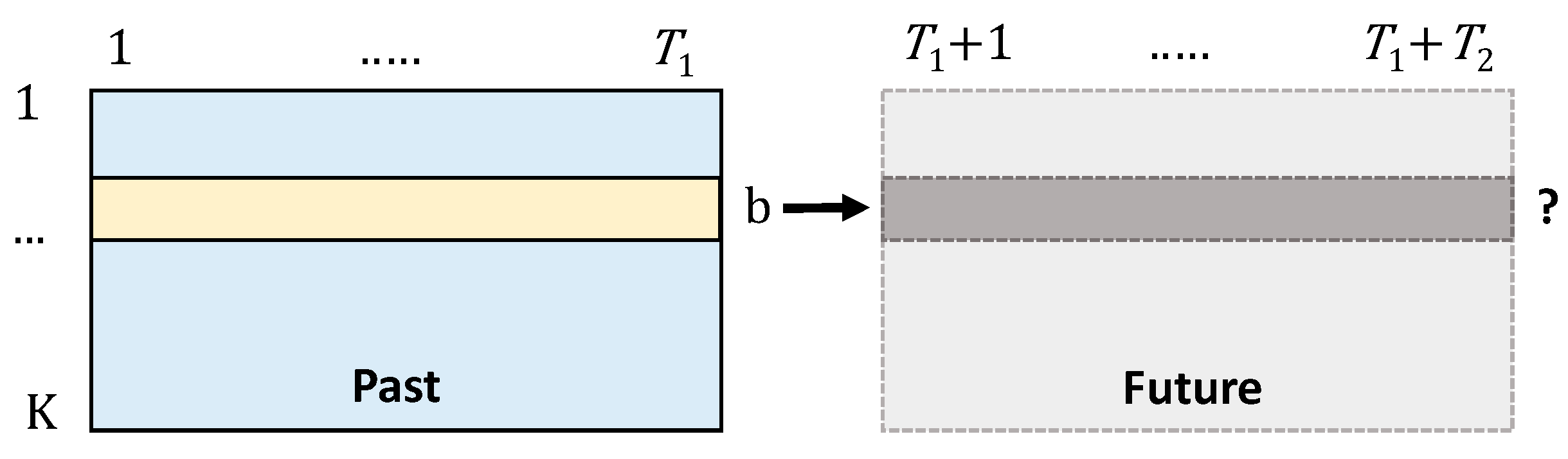
• What is the expected future, i.e., true out-of-sample (OOS) performance (return, SR, etc.) of the best strategy selected on the in-sample (IS), i.e., historical dataset?
• What is the haircut, i.e., the percentage reduction, of the expected OOS performance compared to the IS performance?
• What is the probability of loss, if the strategy is implemented over a future period?
• What is the expected OOS rank of the IS best strategy among the candidate strategies?
• What is the probability that the selected model will in fact underperform most of the candidate models?
• What is the probability that we have selected a false model (false discovery rate—FDR)?

We propose a Bayesian methodology that allows us to simulate many times the IS selection and OOS, i.e., future, realization process (Figure 1) in order to address the questions formulated above. We provide an overview of several methods proposed in the literature that are compared with our method in an empirical study on a set of technical strategies. Since the strategies are basically random and, in fact, we know their performance following the backtesting period, none should be selected. On the other hand, we also artificially modify one of the strategies making it a “true” discovery and analyze results of the strategy selection methods.

2. An Overview of the Existing Approaches

There are several relatively simple classical methods for adjusting p-values in order to accommodate the multiple test (see, e.g., Streiner and Norman 2011). More advanced and computationally demanding methods are based on various approaches to bootstrapping and simulation of the past and future data.

2.1. Classical Approaches

To test significance of a single strategy, for example, ${\mathcal{S}}_b$ with sample mean return $m_b$ and standard deviation $s_b$ observed over $T$ periods, the classical approach is to calculate the t-ratio,

$$TR=\frac{m_b}{s_b/\sqrt{T}},$$

and the two-sided2 p-value,

$$p^S=\mathrm{Pr}\left[\left|X\right|>TR\right],$$

(1)

where $X$ is a random variable following the t-distribution with $T-1$ degrees of freedom. The implicit assumption is that the returns are i.i.d. normal. If the p-value $p^S$ happens to be small enough, e.g., below 5% or 1%, then one tends to jump to the conclusion that a strategy with significantly positive returns has been discovered.

The problem with the process of selecting the best strategy or, alternatively, testing a number of strategies until we find a significant one is that the correct p-value should (Harvey and Liu 2015) reflect the fact that we selected the strategy with the best t-ratio $TR$ out of $K$ proposal strategies.

$$p^M=\mathrm{Pr}\left[\max \left\{\left|X_k\right|,k=1,\dots ,K\right\}>TR\right],$$

where $X_k$ are $K$ random variables following the t-distribution with $T-1$ degrees of freedom (corresponding to the sample t-ratios of the $K$ strategies). It can be noted (Harvey and Liu 2015) that, if the variables were independent, then we could find a simple relationship (also called Šidák’s adjustment) between the single and multiple test p-values.

$$p^M=1-{\displaystyle \prod }_k\mathrm{Pr}\left[\left|X_k\right|\le TR\right]=1-{\left(1-p^S\right)}^K=K{p}^S-\left(\begin{array}{c}K\\ 2\end{array}\right){\left(p^S\right)}^2+\cdots .$$

Harvey and Liu (2015) provided an overview of simple adjustment methods, such as Bonferroni’s adjustment $p^M=\min \{K{p}^S,1\}$, Holm’s, or Benjamini, Hochberg, Zekutieli (BHY) adjustments, using the ordered sequence of the single-test p-values $p_1^S,\dots ,p_K^S$ for all the strategies. The weak point of all those methods is the assumption of independence since the tested strategies are often closely related (e.g., of the same type with varying parameters).

We also propose and test a numerically relatively simple and efficient method on the basis of an estimation of the covariance matrix $\mathsf{\Omega }$ of the returns and numerically generate the distribution of $\max \left\{\left|X_k\right|,k=1,\dots ,K\right\}$ conditional on the null hypothesis $m_k=0$ for all $k$ where $X_k$ are $K$ random variables following the t-distribution with $T-1$ degrees of freedom (or alternatively standard normal for a large $T$) and with covariances given by $\mathsf{\Omega }$.

Note that the classical (corresponding to the basic period, e.g., daily) Sharpe ratio can be easily calculated given the t-ratio and vice versa.

$$S{R}_k=\frac{m_k}{s_k}=\frac{T{R}_k}{\sqrt{T}}.$$

The Sharpe ratio is usually annualized as follows:

$$S{R}_k^a=\frac{m_k}{s_k}\sqrt{T_a}=T{R}_k\sqrt{\frac{T_a}{T}},$$

where $T_a$ is the number of observation periods in a year, e.g., 252 in the case of daily returns. According to Equation (1), the maximal acceptable p-value level can be easily translated to a minimum required Sharpe ratio.

Generally, given a selected strategy with an in-sample (according to the backtest data) Sharpe ratio $S{R}_{IS}$, the question is what the expected (out-of-sample) Sharpe ratio $E_0\left[S{R}_{OOS}\right]$ over a future, e.g., 1-year period, is. Here, $E_0[.]$ denotes the expectation given all the information available today, in particular, given the in-sample performance such as $S{R}_{IS}$, the number of strategies from which the best one was selected, the relationship between the strategies, and the underlying asset return process properties. The Sharpe ratio haircut is then defined as the percentage we need to deduct from the in-sample Sharpe ratio to get a realistic estimate of the future performance,

$$HC=1-\frac{E_0\left[S{R}_{OOS}\right]}{S{R}_{IS}}.$$

(2)

Harvey and Liu (2015) noted that the rule-of-thumb haircut used by the investment industry is 50%, but that, according to their analysis, it significantly depends on the level of the in-sample Sharpe ratio and the number of strategies. They proposed to use the relationship between the single- and multiple-test p-values in order to derive the haircut Sharpe ratio. Their estimate of the annualized expected Sharpe ratio $ES{R}_{HL}$ is based on the idea that its corresponding single-test p-value should be equal to the adjusted multiple test p-value $p^M,$ i.e.,

$$\begin{array}{c}{p}^M=\mathrm{Pr}\left[\left|X\right|>ES{R}_{HL}\sqrt{\frac{T}{T_a}}\right],\mathrm{i}.\mathrm{e}.,\\ ES{R}_{HL}=F^{-1}\left(p^M/2\right)\sqrt{\frac{T_a}{T}},\end{array}$$

where $X$ is a random variable following the t-distribution with $T-1$ degrees of freedom and $F$ is its cumulative distribution function. The haircut is then calculated according to Equation (2). The haircut estimation, of course, depends on the p-value adjustment method as Bonferroni, Holm’s, BHY, or the general one we suggested above. Although the estimation is obviously directionally correct, it is not obvious why this approach should yield a consistent estimate of the expected Sharpe ratio $E_0\left[S{R}_{OOS}\right]$ and of the corresponding haircut. We compare the different haircut estimates in the simulation study outlined below.

2.2. Stationary Bootstrap

In order to simulate the past and the future returns, we consider a bootstrapping and a cross-validation approach. The stationary bootstrap proposed and analyzed in White (2000), Sullivan et al. (1999), and Politis and Romano (1994) is applied to the underlying asset returns assumed to be strictly stationary and weakly dependent time-series to generate a pseudo time series that is again stationary (Figure 2). The tested strategies ${\mathcal{S}}_1,\dots ,{\mathcal{S}}_K$ are based only on the single underlying using its historical returns to take long, short, or possibly zero positions.

Formally, we generate new sequences of the underlying asset returns $\left\{u_{\mathsf{\Theta }\left(\mathrm{i}\right)};i=1,\mathrm{..},\tilde{T}\right\}$ where $u_1,\dots ,u_{T_1}$ is the original series of observed returns and $\mathsf{\Theta }\left(i\right)\in \left\{1,\dots ,T_1\right\}$. In order to implement the bootstrap, we need to select a smoothing parameter $0<q=1/b<1$, where $b$ corresponds to the mean length of the bootstrapped blocks, for example, $q=0.1$, proposed by Sullivan et al. (1999). A bootstrapped sequence is obtained by drawing randomly $\mathsf{\Theta }\left(1\right)\in \left\{1,\dots ,T\right\}$, and, for $i=2,\dots ,\tilde{T}$, setting $\mathsf{\Theta }\left(i\right)=\mathsf{\Theta }\left(i-1\right)+1$ with probability $1-q$ or randomly drawing a new block starting position $\mathsf{\Theta }\left(i\right)\in \left\{1,\dots ,T_1\right\}$ with probability $q$. If it happens that $\mathsf{\Theta }\left(i\right)>T_1$ then we draw random $\mathsf{\Theta }\left(i\right)\in \left\{1,\dots ,T_1\right\}$.

Next, given a bootstrapped sequence of the underlying asset returns, we need to apply strategies ${\mathcal{S}}_1,\dots ,{\mathcal{S}}_K$ to get the strategies’ bootstrapped returns ${\tilde{r}}_{k,t},k=1,\dots ,K,t=1,\dots ,T_1$. Note that, since the strategies’ decisions are built on the basis of past returns, we generally need to have a longer series of the bootstrapped asset returns, $\tilde{T}>T_1,$ where $T_1$ is the length of the in-sample period. Then, we evaluate our desired performance indicator values (mean return, Sharpe ratio, etc.) ${\tilde{f}}_k$. Let $f_k^{*}$ denote the performance indicators of the original series of returns. According to White (2000), under certain mild theoretical assumptions, the empirical distribution of the $B$ bootstrapped values $\widetilde{V_j}=\underset{\mathrm{k}=1,\dots ,\mathrm{K}}{\max }\left({\tilde{f}}_k-f_k^{*}\right)$ for $j=1,\dots ,B$ asymptotically converges to the distribution of the best strategy performance indicator under the null hypothesis $H_0$ that all the strategies have zero performance. That is, obtaining $B$ bootstrapped values $\left\{{\tilde{V}}_j;j=1,\dots ,B\right\}$, we can test $H_0$ by calculating the empirical p-value $\mathrm{Pr}\left[\left|{\tilde{V}}_j\right|>f_b^{*}\right]$, where $b$ is the index of the best strategy and $f_b^{*}=\underset{k}{\max }{f}_k^{*}$.

The bootstrap technique can be also used to analyze the relationship between IS and OOS Sharpe ratio (or another indicator), generating series of strategy returns over a time period $1,\dots ,T_1$, selecting the best strategy ${\mathcal{S}}_b$ with an in-sample performance $S{R}_{IS}$, and then looking at its out-of-sample performance $S{R}_{OOS}$over the following period $T_1+1,\dots ,T_1+T_2$. Note that, in this case, the original bootstrapping must be done over a period of length $\tilde{T}>T_1+T_2$. Then, we can compare the mean $S{R}_{OOS}$against the mean $S{R}_{IS}$ or conditional on certain level of $S{R}_{IS}$. We may also bootstrap the OOS returns for the actually selected strategy ${\mathcal{S}}_b$ (according to the real dataset). However, in this case, it is especially obvious that even a truly positive strategy that is using medium-term or long-term trends to make good predictions does not have to work on the bootstrapped series of returns where the future and past returns of the original series are to a large extent mixed up. Therefore, the estimated conditional $S{R}_{OOS}$may easily lead to a false rejection of a positive strategy.

2.3. Combinatorial Symmetric Cross-Validation

Another disadvantage of the stationary bootstrap technique is that it cannot be applied if we are given only the strategy returns but not details on the strategies themselves. The stationary bootstrap is also problematic if the strategies are not technical ones and use a number of additional, possibly lagged, explanatory factors. This is not the case for the combinatorial symmetric cross-validation (CSCV) (Bailey et al. 2014, 2016) utilizing only the matrix of the strategies’ returns $M=\left\{r_{k,t}, k=1,\dots ,K, t=1,\dots ,T_1\right\}$. The idea is to split the time window of length $T_1=SN$ into $S$ blocks of length $N$, where $S$ is even and draws combinations of $S/2$ blocks (Figure 3). The submatrix $J$ formed by joining $T_1/2$ rows of $M$ corresponding to the selected time indices in the original order then represents an in-sample dataset of returns where the best performing strategy can be selected while the complementary $K\times T_1/2$ submatrix $\overline{J}$represents the out-of-sample returns. The sampling can be done with or without replacement. Since there are $\left(\begin{array}{c}S\\ S/2\end{array}\right)$ combinations, we can sufficiently form many different combinations with replacement as long as $S$ is sufficiently large, e.g., at least 16.

Bailey et al. (2014, 2016) proposed using the technique to specifically estimate the probability of backtest overfitting (PBO) defined as the probability that the best IS selected strategy performs below the average OOS. More precisely, for $K$ strategies ${\mathcal{S}}_1,\dots ,{\mathcal{S}}_K$,

$$PBO=\mathrm{Pr}\left[Ran{k}_{OOS}\left(X\right)<K/2|Ran{k}_{IS}\left(X\right)=1\right].$$

The PBO indicator, as well as the Sharpe ratio haircut, can be estimated using sufficient cross-validation pairs of the IS/OOS datasets $\langle J,\overline{J}\rangle$. However, it is obvious that the estimates are biased, introducing a negative drift into the OOS order of the strategies. For example, if all the strategies represented just pure noise with mean returns over the full time interval $\left\{1,\dots ,T_1\right\}$ close to zero, then, for an IS/OOS combination $\langle J,\overline{J}\rangle$, the best strategy IS return ${\overline{r}}_{b,J}$ implies that the complementary OOS return ${\overline{r}}_{b,\overline{J}}\approx -{\overline{r}}_{b,J}$ would probably be the worst on $\overline{J}$. We demonstrate the effect in the empirical section. The cross-validation technique also cannot be used, due to this property, to estimate the OOS Sharpe ratio or mean for a particular selected strategy. We can just estimate the overall $PBO$ or Sharpe ratio haircut keeping in mind that the estimations incorporate a conservative bias. The cross-validation, as well as the bootstrapping approach, cannot be easily used to estimate the false discovery rate (FDR) since it is not clear how to identify true and false discoveries given a CSCV simulation. This could be possibly done by testing the significance of OOS performance involving an ad hoc probability level.

We show that all the indicators of interest can be consistently estimated in the Bayesian setup outlined below.

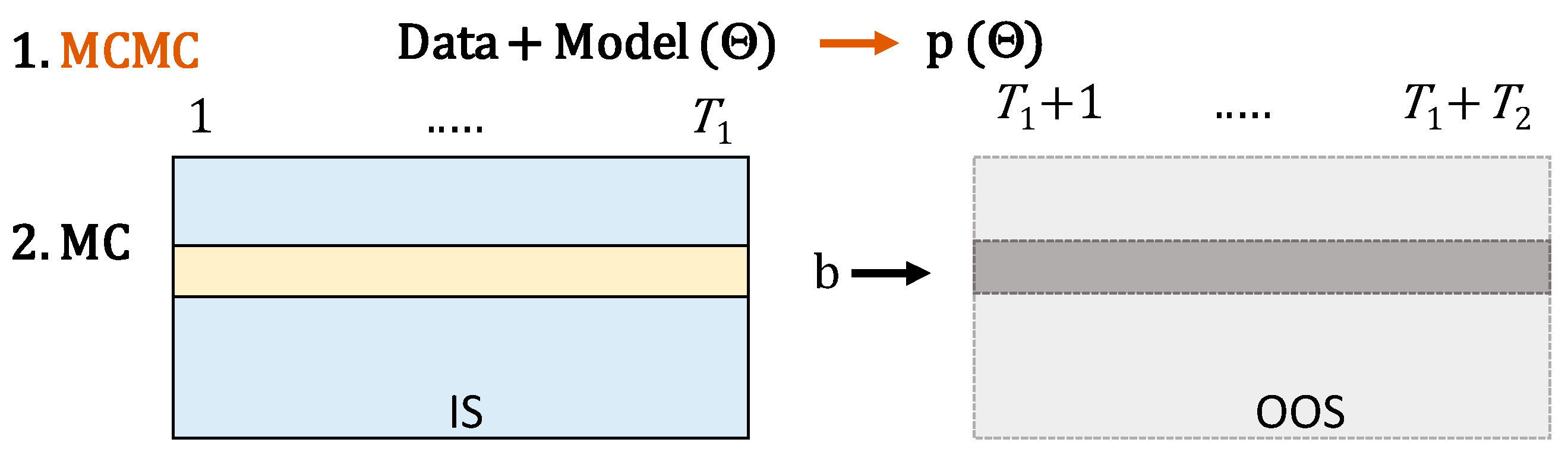
3. Bayesian Simulation Approach

The Bayesian approach is based on the scheme given in Figure 4.

First, of course, we need to specify a model defining the return generating process with unknown parameters $\mathsf{\Theta }$ for the observed strategy returns $\left\{r_{k,t}, k=1,\dots ,K, t=1,\dots ,T\right\}$, where $T=T_1$ or $T=T_1+T_2$. Then, the plan is to use a Bayesian technique, specifically, the Markov Chain Monte Carlo (MCMC) simulation, in order to extract the posterior distribution of the model parameters $\mathsf{\Theta }$. Finally, we simulate the matrices of IS and OOS returns over desired time intervals $1,\dots ,T_1$ and $T_1+1,\dots ,T_1+T_2$. The Monte Carlo (MC) is done in two steps, always selecting the parameters $\mathsf{\Theta }$ from the posterior distribution and then generating $K$ series of $T_1+T_2$ returns according to the model. The simulated IS returns can be used to select the best strategy and the OOS returns to measure its future performance. The average haircut or average relative rank can be easily estimated as in the case of the stationary bootstrap (see Figure 4).

We consider two models; the simple one assumes that the returns are multivariate normal with unknown covariance matrix and means, while the second incorporates unknown indicators of truly profitable strategies allowing us to consistently estimate the false discovery rate (FDR). The second model follows an idea of Scott and Berger (2006), also mentioned in Harvey et al. (2016); nevertheless, in both cases, the model was formulated only for observed mean returns and without considering a correlation structure of returns. It should be emphasized that our focus is to analyze the impact of backtest overfitting assuming that the strategies’ cross-sectional returns behave in a relatively simple and stable way over time similarly to the classical, bootstrapping, or cross-validation approaches. One could certainly come up with state-of-the-art models incorporating jumps, switching regimes, stochastic variances, or even dynamic correlations. These improvements would make the methodology computationally difficult to manage with results probably even more conservative compared to the approaches we consider below.

3.1. The Naïve Model 1

To set up the naïve model, we assume that the cross-sectional strategy returns are multivariate normal,

$${\mathit{r}}_t=\langle r_{1,t},\dots ,r_{K,t}\rangle \sim N\left(\mathit{\mu },\Sigma \right),$$

and that the observations over time are independent.

Given $\mathrm{data}= \langle r_t\rangle$, i.e., the matrix of back test returns, and possibly some priors for $\mathit{\mu }$ and $\Sigma$, we can find the posterior distribution $p(\mathit{\mu },\Sigma |\mathrm{data})$ using the standard Gibbs MCMC sampler.

Specifically, the iterative sampling is given by

$$\begin{array}{c}p\left(\mathit{\mu }|\Sigma ,\mathrm{data}\right)=\mathsf{\phi }\left(\mathit{\mu };\frac{1}{\mathrm{T}}{{\displaystyle \sum }}_{t=1}^T{\mathit{r}}_t,\frac{1}{T}\Sigma \right),\mathrm{and}\\ p\left(\Sigma |\mathit{\mu },\mathrm{data}\right)=IW\left(\Sigma ;T,S\right),\end{array}$$

where $S={\displaystyle \sum }_{t=1}^T\left({\mathit{r}}_t-\mathit{\mu }\right){}^{\prime }\left({\mathit{r}}_t-\mathit{\mu }\right)$ is the scale matrix (i.e., the covariance matrix times $T$), and $IW$ is the inverse Wishart distribution. For example, Matlab allows sampling from the distributions, and the posterior distribution may be obtained quite efficiently (e.g., 10,000 runs of the sampler).

Remark 1.

The sampler above assumes the noninformative prior on the means,$p\left(\mathit{\mu }\right)\propto 1$, and the standard improper prior on the covariance matrix,

$$p\left(\Sigma \right)\propto {\left|\Sigma \right|}^{-\frac{K+1}{2}}.$$

Given the extracted posterior distribution $p\left(\mathit{\mu },\Sigma |\mathrm{data}\right)$, the parameters $\mathit{\mu },\Sigma$ can be now easily sampled in order to get the empirical distribution of the selected strategy performance. However, in the process of selecting the best strategy, we do not know $\mathit{\mu },\Sigma$ but only a time series of the backtested returns with cross-sections from $N\left(\mathit{\mu },\Sigma \right)$. On the basis of the time series, the “best” strategy${\mathcal{S}}_b$ is selected. Our key question is about its expected forward-looking performance, e.g., ${\mu }_b$ or $S{R}_b$. Therefore, we need to run the following Monte Carlo simulation in order to faithfully sample the empirical distribution of the performance indicators:

• Sample $\langle \mathit{\mu },\Sigma \rangle$ from $p(\mathit{\mu },\Sigma |\mathrm{data})$.
• Independently sample $T_1+T_2$ cross-sections $R_t\sim N\left(\mathit{\mu },\Sigma \right)$.
• Determine the index of the best strategy $b$ on the basis of the backtest statistics calculated from the matrix of backtested returns $\mathit{R}=\langle {\mathit{R}}_t\rangle$ for $t=1,\mathrm{..},T_1$.
• Calculate and store the performance indicators, ${\widehat{\mu }}_b,$ $\widehat{S{R}_b}$, in the OOS period $T_1+1,\dots ,T_2.$ Alternatively, store the selected strategy “true” performance indicators, i.e., ${\mu }_b,$ $S{R}_b$.

The MCMC estimation of the multivariate normal distribution parameters is known to converge relatively fast (see e.g., Lynch 2007); nevertheless, we apply a burn-out period according to simple diagnostics, e.g., the average of the vector of mean returns $\mathit{\mu }$. The simulated posterior distribution of the desired performance indicators (after removing the burn-out period) then tells us the mean, median, confidence intervals, or Bayesian probabilities where the true performance is positive or above any given minimum threshold. The ratio between the ex post and ex ante performance indicators also gives us an estimate of the “backtest overfitting haircut”.

3.2. Model 2—Bimodal Means Distribution

In order to capture the situation when most strategies are random and only some positive (nonzero), assume that there are, in addition, latent indicators ${\gamma }_i\in \left\{0,1\right\}$ so that the mean of strategy $i$ is ${\mu }_i^{*}={\gamma }_i{\mu }_i$. Therefore, the row vector of returns has the distribution

$${\mathit{r}}_t=\left[r_{1,t},\dots ,r_{K,t}\right] \sim N\left({\mathit{\mu }}^{*},\Sigma \right).$$

Here, we need to assume a prior distribution for ${\gamma }_i\sim Bern\left(1-p_0\right)$ and ${\mu }_i\sim N\left(m_0,V_0\right)$. It means that the Bayesian distribution of the means is bimodal with a large probability mass on 0, and the other mode is normal with prior mean $m_0>0$ and variance$V_0$. The Gibb’s sampler can be modified as follows:

• Given $\mathit{\mu },\mathit{\gamma }$, set ${\mu }_i^{*}={\gamma }_i{\mu }_i$, and estimate $\Sigma$ as above, i.e.,

  $$p\left(\Sigma |\mathit{\mu },\mathit{\gamma }, \mathrm{data}\right)=IW\left(\Sigma ;T,S\right),\mathrm{where}S={{\displaystyle \sum }}_{t=1}^T\left({\mathit{r}}_t-{\mathit{\mu }}^{*}\right){}^{\prime }\left({\mathit{r}}_t-{\mathit{\mu }}^{*}\right).$$
• Given $\Sigma , \mathit{\gamma }$, estimate $\mathit{\mu }$. Set $A=\frac{1}{T}\Sigma$, $\mathsf{\Gamma }=diag\left(\mathit{\gamma }\right)$, $\mathit{m}=\frac{1}{T}{\displaystyle \sum }_{t=1}^t{\mathit{r}}_t$, ${\mathit{m}}_0=\left[m_0,\dots ,m_0\right]$, and $D=diag\left(\left[V_0,\dots ,V_0\right]\right)$, where $diag$ creates a matrix with diagonal elements given by the vector in the argument, and sample

  $$p\left(\mathit{\mu }|\Sigma ,\mathit{\gamma },\mathrm{data}\right)=\mathsf{\phi }\left(\mathsf{\mu };\left(\mathsf{\Gamma }{A}^{-1}\mathsf{\Gamma }+{\mathrm{D}}^{-1}\right)\left({\mathsf{\Gamma }\mathrm{A}}^{-1}\mathit{m}+D^{-1}{m}_0\right),{\left(\mathsf{\Gamma }{A}^{-1}\mathsf{\Gamma }+{\mathrm{D}}^{-1}\right)}^{-1}\right).$$
• Given $\Sigma$ and $\mathit{\mu }$, estimate $\mathit{\gamma }$. For $i=1,\dots ,K$ set ${\mathsf{\Gamma }}_0$ equal to $\mathsf{\Gamma }$ with the exception of the diagonal element ${\mathsf{\Gamma }}_0\left(i,i\right)=0$, and ${\mathsf{\Gamma }}_1$ setting ${\mathsf{\Gamma }}_1\left(i,i\right)=1$. Let

  $$L_0=\exp \left(\frac{-1}{2}\left(\left({\mathsf{\Gamma }}_0\mathit{\mu }-\mathit{m}\right){}^{\prime }{A}^{-1}\left({\mathsf{\Gamma }}_0\mathit{\mu }-\mathit{m}\right) \right)\right)\left(1-p_0\right),$$

  $$L_1=\exp \left(\frac{-1}{2}\left(\left({\mathsf{\Gamma }}_1\mathit{\mu }-\mathit{m}\right){}^{\prime }{A}^{-1}\left({\mathsf{\Gamma }}_1\mathit{\mu }-\mathit{m}\right) \right)\right)p_0,$$

  $$\tilde{p}=\frac{L_1}{L_0+L_1},\mathrm{and}\mathrm{finally},\mathrm{sample}{\gamma }_i\sim Bern\left(\tilde{p}\right).$$

Proofs of the formulas used in steps 2 and 3 can be found in Appendix A. Again, we apply a burn-out period according to a convergence diagnostic of the averages of $\mathit{\gamma }$and of $\mathit{\mu }$.

Remark 2.

There are certain possible extensions.

• We may allow${\gamma }_i\in \left\{-1,0,1\right\}$encoding negative significant mean return, zero return, or significant positive return. In this case, the mean parameter of the prior distribution${\mu }_i\sim N\left(m_0,V_0\right)$must be strictly positive. In the Gibb’s sampler above, we just need to modify step 3 in a straightforward manner.
• The hyper-parameters$p_0,m_0,V_0$for${\gamma }_i\sim Bern\left(1-p_0\right)$and${\mu }_i\sim N\left(m_0,V_0\right)$might be estimated within the MCMC procedure. In this case, the Gibb’s sampler can be extended as follows:

  4.

  Sample$p_0$given$\mathit{\gamma }$:

  $$p\left(p_0|\mathit{\gamma }\right)\propto p_0^{n_1}{\left(1-p_0\right)}^{1-n_1}p\left(p_0\right)\propto Beta\left(p_0;n_1+k1+1,K-n_1+k2+1\right),$$

  where$n_1=\#\left\{i;{\gamma }_i=1\right\}$and$p\left(p_0\right)=Beta\left(p_0;k1+1,k2+1\right)$is a conjugate prior distribution (e.g.,$k_1=k_2=1)$.

  5

  Sample$m_0,V_0$given$\mathit{\mu }$and$\mathit{\gamma }$. Here, we just use the means$\left\{{\mu }_i\right|{\gamma }_i=1\}$where the signal is positive and the normal Gibb’s sampler. Since the set may be empty, we need to use proper conjugate priors, e.g.,$p\left(m_0\right)=\phi \left(m_0;0,m_P\right)$and

  $$\left(V_0\right)\propto IG\left(V_0,\frac{k_0}{2},\frac{k_0{V}_P}{2}\right).$$
  For$\tilde{K}=\#\left\{{\mu }_i\right|{\gamma }_i=1\}\ne 0$, set$\tilde{\mu }=\sum \left\{{\mu }_i\right|{\gamma }_i=1\}/\tilde{K}$and$\tilde{V}=\sum \left\{{({\mu }_i-m_0)}^2\right|{\gamma }_i=1\}/\tilde{K}$. Then,

  $$\begin{array}{c}p(m_0|\mathit{\mu }, \mathit{\gamma },V_0)\propto \phi (m_0;\tilde{\mu },V_0/\tilde{K}) \phi \left(m_0;0,V_P\right)\propto \phi \left(m_0;\frac{\tilde{\mu }\tilde{K}{V}_P}{\tilde{K}{V}_P+V_0},\frac{V_P{V}_0}{\tilde{K}{V}_P+V_0}\right)\mathit{and}\\ p(V_0|\mathit{\mu }, \mathit{\gamma },m_0)\propto IG\left(0;\frac{\tilde{K}}{2},\frac{\tilde{K}\tilde{V}}{2}\right) IG\left(V_0,\frac{k_0}{2},\frac{k_0{V}_P}{2}\right)\propto IG\left(V_0,\frac{\tilde{K}+k_0+1}{2},\frac{\tilde{K}\tilde{V}+k_0{V}_P}{2}\right).\end{array}$$
  If$\tilde{K}=0$. then we have to sample on the basis of conjugate priors$p\left(m_0\right)$and$p\left(V_0\right)$only.

4. Numerical Study

Following Sullivan et al. (1999) and other studies, we compare and illustrate the proposed Bayesian methods on a set of technical strategies’ returns. We also artificially modify the mean returns of the strategies in order to test the methods, on one hand, if there is a clearly extraordinary strategy or, on the other hand, if the returns of the returns of all the strategies are very low.

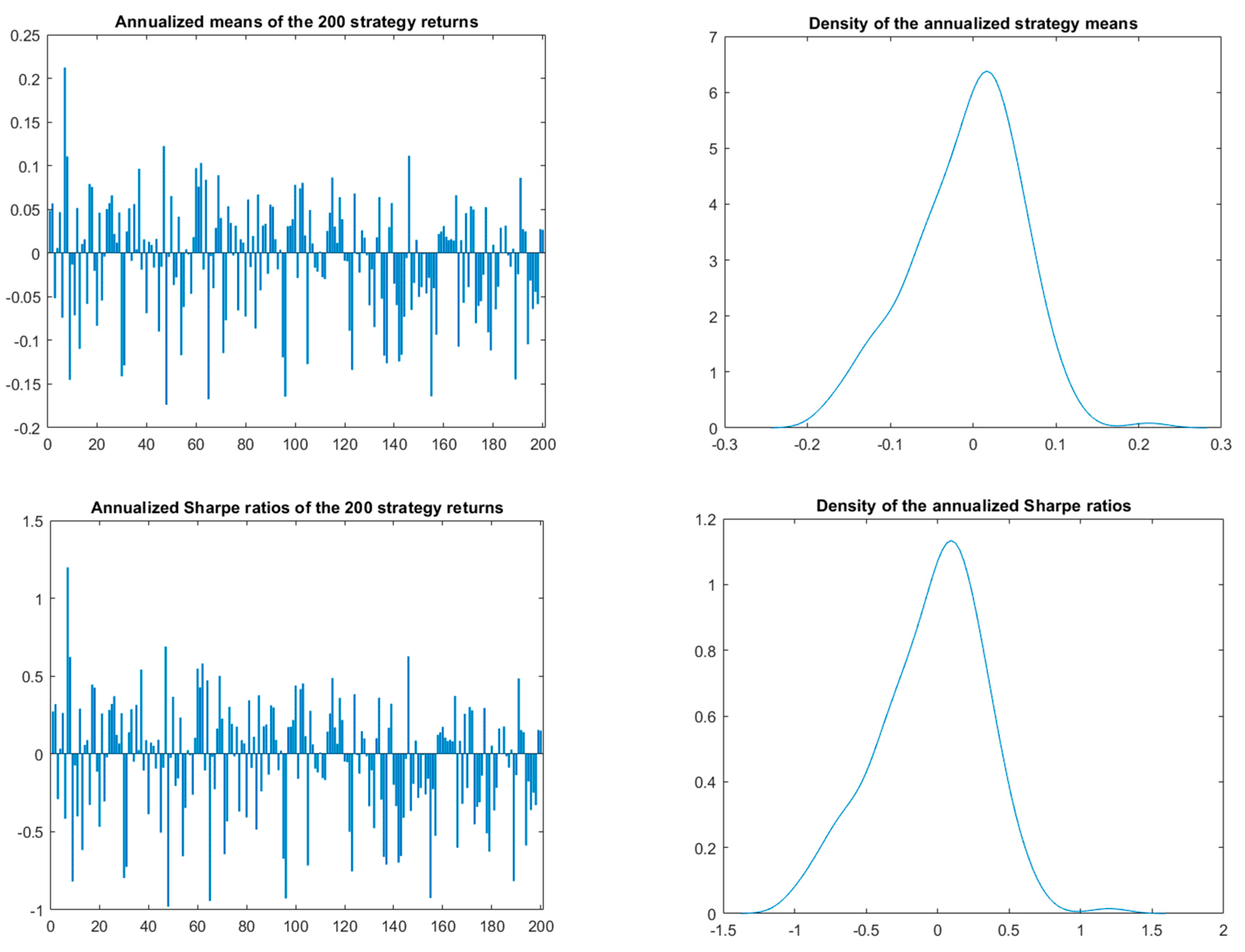
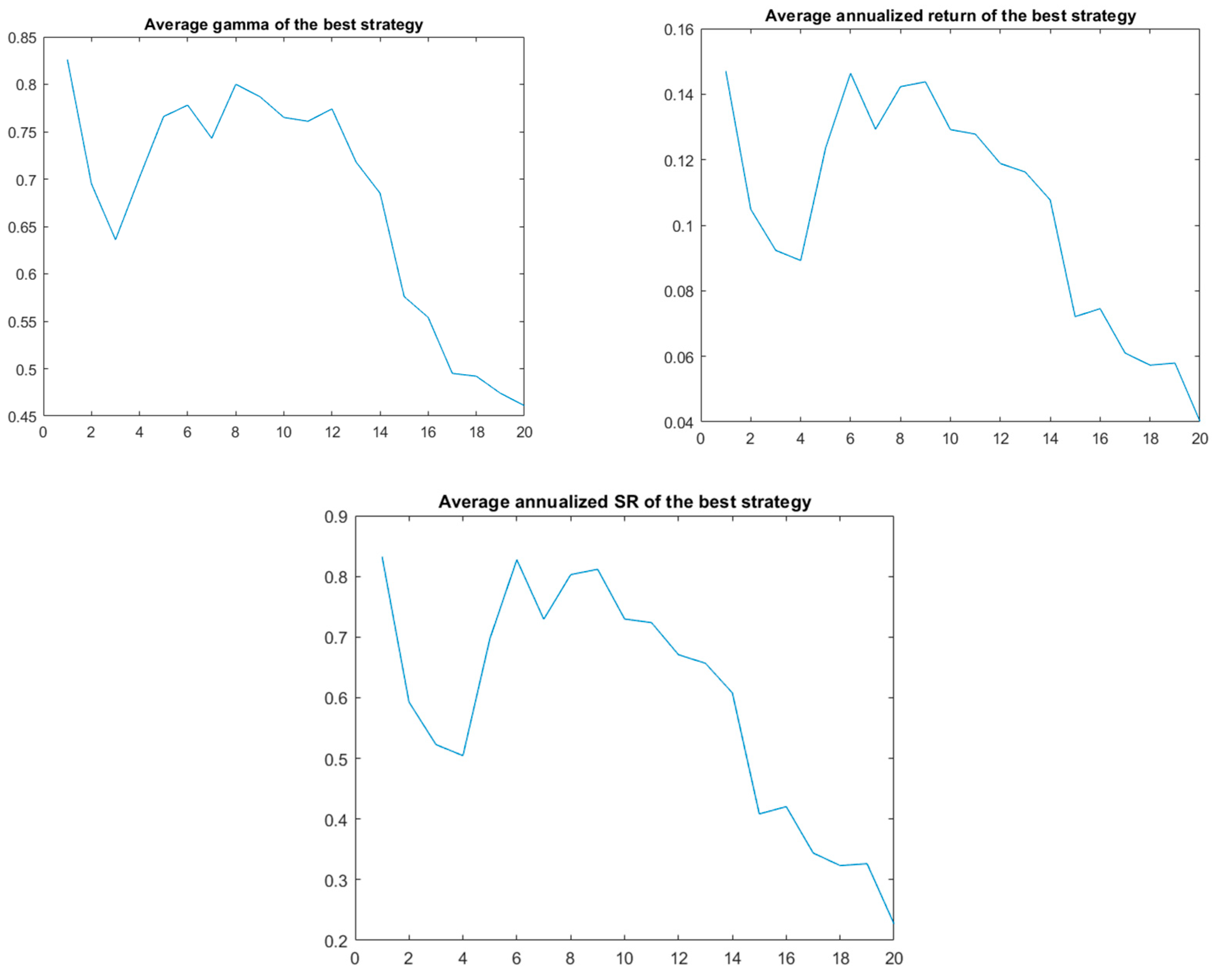
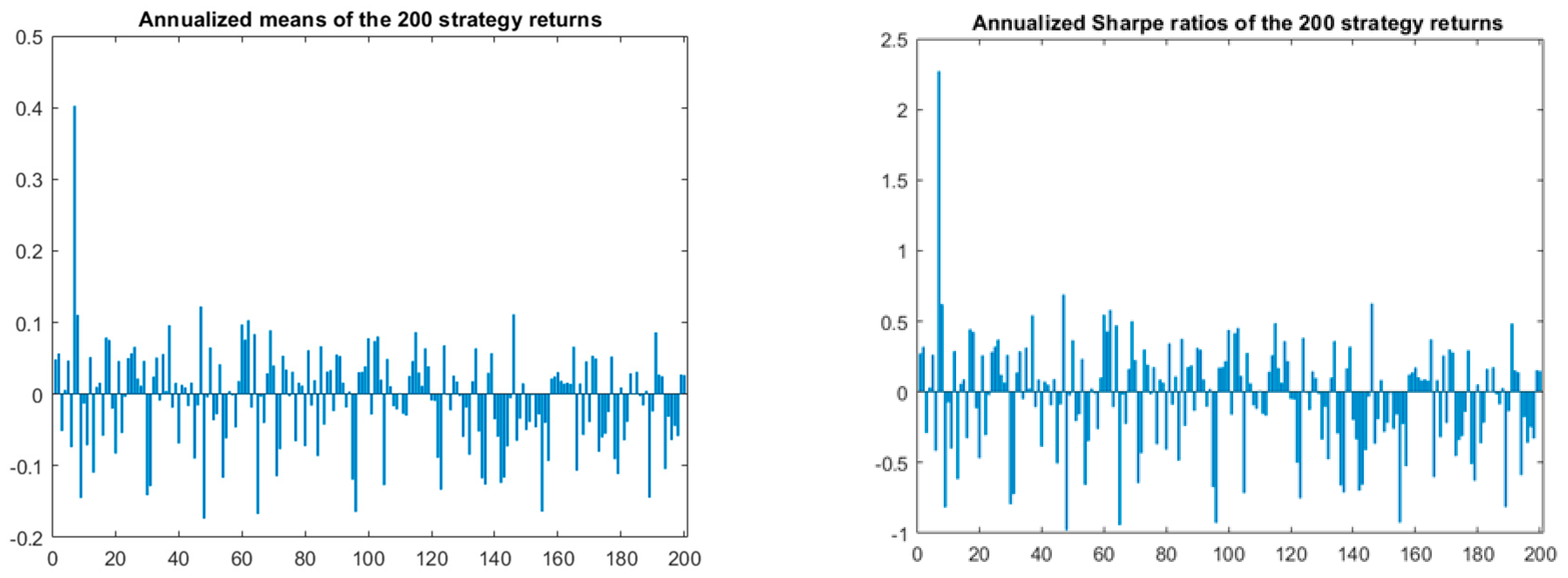
4.1. Technical Strategies Selection

We used 1000 daily S&P 500 values and returns for the period 5 June 2009–24 May 2013 (1000 trading days). The period was selected with the purpose of finding at least one strategy with a higher mean return. As in Sullivan et al. (1999), we applied the filter, moving average, support, and resistance rules with varying parameters. We randomly selected 200 strategies with the condition that the daily return series are not collinear (it may even happen that the series are identical if the parameters do not differ too much).

The means and Sharpe ratios of the individual strategies’ return series and their densities over the period 5 June 2009–24 May 2013 are shown in Figure 5. It should not be surprising that the strategies’ returns are mostly positively correlated with the average pairwise correlation 23.32%. Note that strategy 7 is apparently the best with the annualized ($n_y=252$) mean return over 21% p.a. and Sharpe ratio approximately 1.2 (it is a filter strategy with x = y = 1%, i.e., a long or short position is taken if the previous daily return is over 1% or below −1%, respectively, and the minimum number of days to stay in a position is 20). The strategy returns look attractive; nevertheless, looking forward, it turns out that the realized mean return of the strategy in the 1000 days following 24 May 2013 is negative (−5.21%).

4.2. Single and Multiple p-Value Testing

The single-test annualized t-ratio and the p-value of the best strategy 7 with $SR=1.1987$ are

$$TR=SR\sqrt{\frac{n_{obs}}{n_y}}=1.1987\sqrt{1000/252}=2.3878\mathrm{and}{p}^S=0.0171.$$

The multiple test p-value after Bonferroni adjustment is simply

$$p^M=\min \left\{200\times 0.171,1\right\}=1.$$

Thus, the adjusted expected Sharpe ratio is 0 and the haircut is 100%. Šidák’s adjustment yields only a slightly more optimistic result with $p^M=0.9685$, adjusted expected $SR=0.02$, and haircut 98.3%. Similar adjustments can be obtained by the Holm or Benjamini, Hochberg, Yekutieli (BHY) methods using, for example, the package provided by Harvey and Liu (2015). The simple adjustment methods allow to easily estimate the minimum return of the best strategy (keeping the same covariance structure) in order to get the multiple test p-value at most 5%. The estimated minimum return using the same package is around 36%.

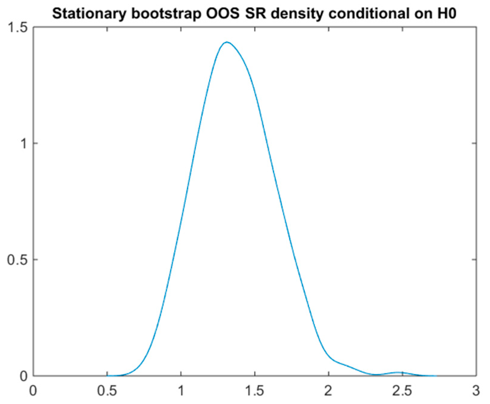
4.3. Multivariate Normal Simulation and the Stationary Bootstrap According to the Null Hypothesis

Another relatively simple possibility is to estimate the return covariance matrix and simulate the future multivariate returns on the basis of the return covariance matrix and conditional on zero means. Figure 6 below shows the density of 1000 simulated annualized SR as a function of a 1000 day period. The adjusted p-value of the best strategy with $SR=1.1987$ is then relatively optimistic 0.352 and the adjusted expected SR is 0.4683 (i.e., the implied haircut is just 61%).

An analogous distribution (Figure 7) can be obtained via the much more computationally demanding stationary bootstrap (White’s reality check). The p-value according to 1000 bootstrap simulations for a 1000-day time period and with $q=0.1$ turns out to be 0.728, the corresponding adjusted expected SR is 0.175, and the SR haircut is 85.4%.

4.4. Stationary Bootstrap Two-Stage Simulation

The stationary bootstrap method can also be used to simulate the backtest period of length $T_1=1000$, as well as the future period with $T_2=1000$. The number of stationary bootstrap iterations is again 1000 according to the 5 June 2009–24 May 2013 window of S&P returns, and the parameter is set to $q=0.1$ with the corresponding average length of the bootstrapped blocks being 10. Figure 8 shows the typical strong shift of the ex ante performance density to the left-hand side and the wider ex post performance density. The results show that the best IS selected strategy performs poorly OOS with 32.8% probability of loss, PBO around 0.44 (see also Figure 9), and SR haircut over 73%. For detailed results including the ex ante and ex post SR or mean return values, see the summary in

Table 1. Summary of the backtest overfitting tests’ results.

	Adjusted p-Value (FDR)	Ex Ante av. SR/Mean	Adjusted Expected SR/Mean	SR/Mean Hair Cut	Probability of Loss	Mean OOS Rank	PBO
Boferroni method	1.00	1.199	0	100%	-	-
Šidák’s correction	0.968	1.199	0.02	98.3%	-	-
Mult. norm. MC adj.	0.352	1.199	0.4668	61%	-	-
Stationary bootstrap	0.728	1.110/0.194	0.297/0.051	73.2%/74%	0.328	55%	0.444
CSCV	-	1.382/0.244	0.336/0.058	75.7%/76.4%	0.371	66.8%	0.323
Bayes mod. 1	-	2.102/0.371	1.014/0.180	51.8%/51.5%	0.171	75.7%	0.168
Bayes mod. 2	0.549	1.201/0.213	0.211/0.037	82.5%/82.5%	0.380	60%	0.395

. Note that the row “stationary bootstrap” shows values obtained via the two-stage simulation except the p-value estimated by White’s reality check.

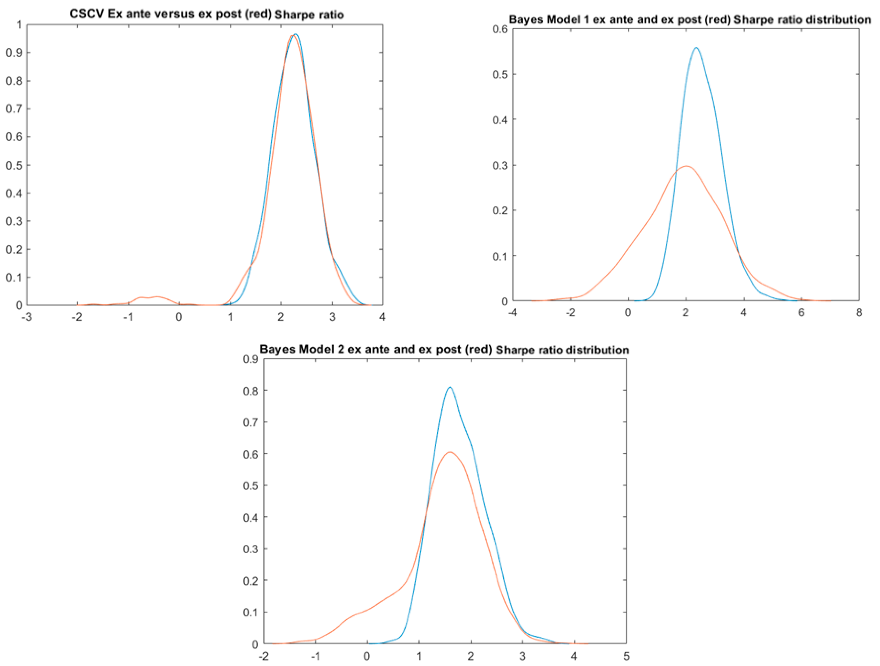
4.5. Combinatorial Symmetric Cross-Validation

In order implement the CSCV algorithm, we chose the number of blocks 20 corresponding to

$$\left(\begin{array}{c}20\\ 10\end{array}\right)=184,756$$

combinations of 10 blocks of length 50. However, we sampled only 1000 combinations. In this case, we always split the 1000-day time into the IS and OOS parts on the same length, i.e., $T_1=500$ and $T_2=500$. The results shown in Table 1 are quite like the stationary bootstrap only with PBO being slightly lower (0.323). The slightly better performance is reflected in the bimodal ex post densities in Figure 10 where the right-hand side positive mode corresponds to the selected strategy that performs well IS, as well as OOS. Figure 11 also indicates that, in this case, compared to Figure 9, the best IS strategy remains the best OOS quite often.

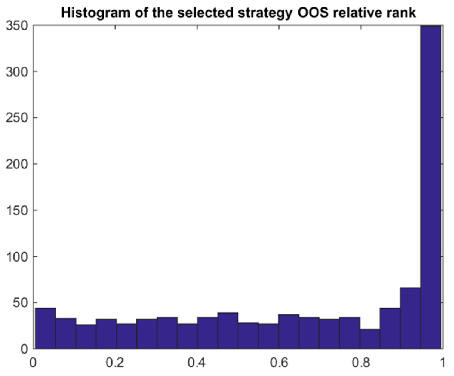
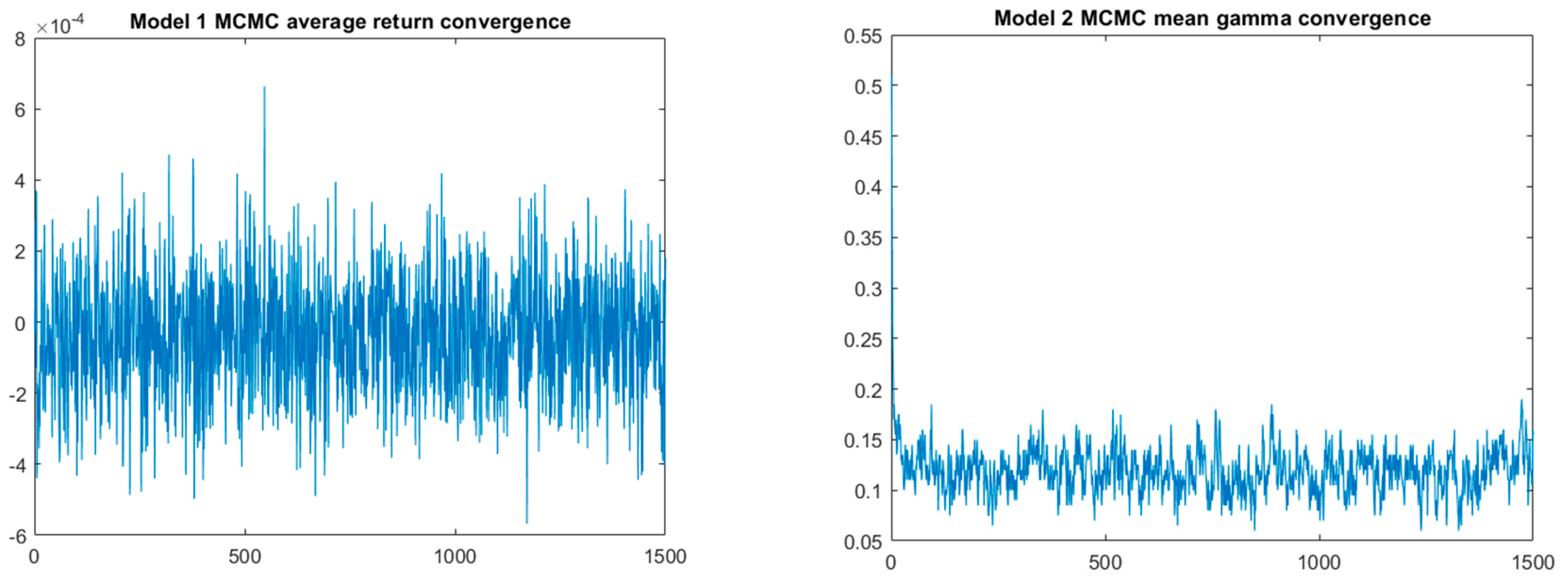
4.6. The Naïve Bayes Model 1

In the Bayesian approach, we firstly extract the multivariate normal model means and covariance given the observed data. This can be done in 1500 iterations using the standard Gibbs sampler including 500 burn-out simulations, i.e., only the last 1000 iterations are used to estimate the posterior parameters (see Figure A1, Appendix A, for the fast MCMC convergence). In the MC simulation, we can choose the length of the backtest (IS) period $T_1=1000$and the OOS forward looking period $T_2=1000$. We then generated 1000 scenarios (after removing the burned-out simulations) sampling the parameters and the cross-sectional returns, selecting the best IS strategy, and measuring its OOS performance. We have to keep in mind that the sampled posterior means may differ quite significantly from the observed mean returns due to the high return volatility3 and, thus, the observed best strategy 7 may look weak in the simulations, while other strategies are selected as the best. The detailed results given in Table 1 and Figure 12 confirm that the naïve multivariate normal model indeed appears too optimistic. Indeed, the best IS strategy remains the best quiet often as shown in Figure 13 and the PBO is quite low (0.168). This can be explained by the simple multivariate normal model and relatively long IS window allowing to identify the truly positive strategy.

In reality, if we generate a large number of models and the best model performance is still poor, then we are probably not going to enroll it for real trading. Therefore, we might also consider a minimum hurdle at which we choose or reject the best selected model. This is quite easy given the simulation outputs. For example, if we set the minimum SR to 1.2, then the condition will be satisfied in 96.6% of the simulations with average ex ante SR 2.14 and ex post SR 1.00, i.e., again with the haircut slightly over 53%. It is interesting that the haircut is not much sensitive to the hurdle, e.g., if the minimum SR was 2, then the corresponding average haircut would be even higher (37%). Nevertheless, the probability of loss can be reduced by setting the minimum SR higher, e.g., if we set the hurdle to 2, then the conditional probability of loss would decline to 16.5% (conditional on the strategy selection) and the unconditional probability would decline to 9.1% since 44.9% of the proposed models would be rejected in the simulation.

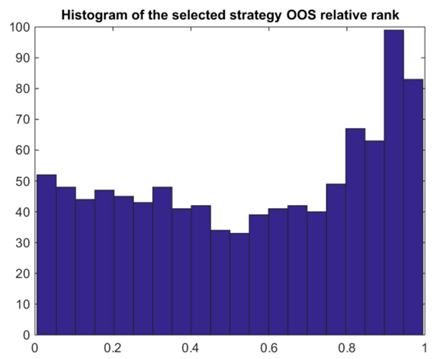
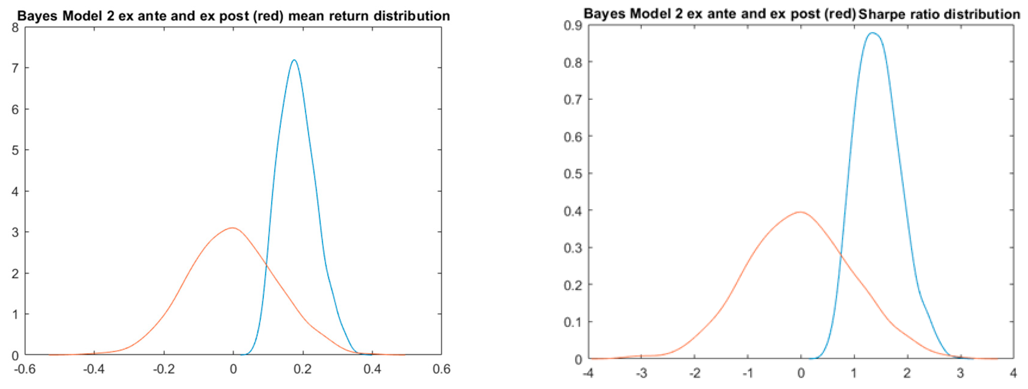
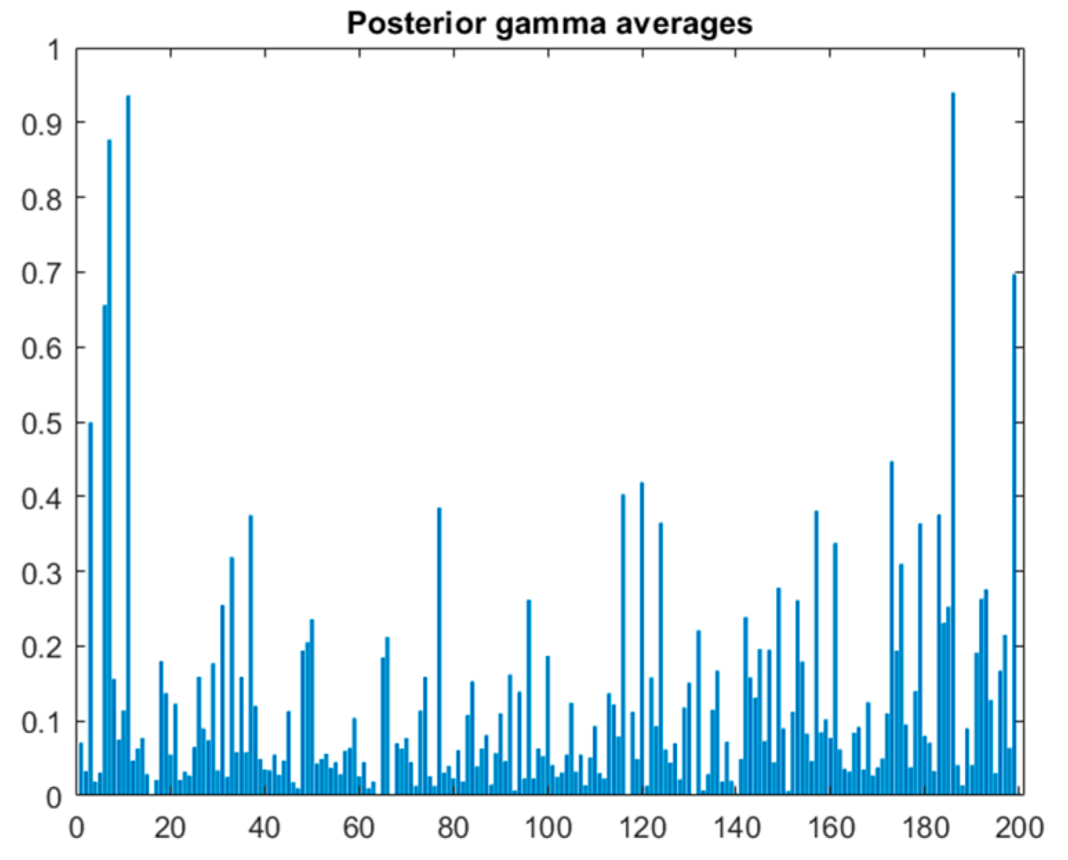
4.7. Bayes Bimodal Mean Returns Model 2

In this case, in addition to the multivariate normal distribution with unknown parameters, we also consider latent indicators of zero and nonzero models. In order to extract the posterior distribution of the parameters and the latent indicators, we again run 1500 iterations and use only the last 1000 iterations to estimate the parameters (removing first 500 burn-out iterations—see Figure A1, Appendix A, for the relative MCMC convergence) of the Gibbs sampler outlined in Section 3.2. Analogously to Bayes Model 1, we then run 1000 Monte Carle simulations with T₁ = 1000 and T₂ = 1000. Since, in this case, the Bayesian model incorporates the uncertainty whether the model is a true discovery or not, the results should be more conservative compared to the naïve model. Indeed, the PBO turns out to be 0.395, substantially lower compared to model 1, the SR haircut is 82.5%, and the probability of loss is 38% (see Table 1, Figure 14 and Figure 15).

The model also provides posterior averages of γ_i for each individual model i (see Figure 16). The averages can be interpreted as Bayesian probabilities that the models are true discoveries. There are a few models with the averages over 80%, including the model 7 with the value over 86%. The complements of these Bayesian probabilities to 100% can be in a certain sense compared to the frequentist single-test p-values. However, the Bayesian model also allows us to answer the key question we are asking: Given the observed data and the general model assumptions, what is the probability that the best strategy b selected on the basis of observed data is a true discovery, i.e., γ_b = 1? This can be estimated as the mean of γ_b which turns out to be only 0.459. This means that, applying the selection process, we identify the true discovery only in 45.1% of cases and we make a false discovery in 54.9% of cases, i.e., FDR = 54.9% can be shown instead of the adjusted p-value in Table 1.

We may again test whether a higher SR hurdle reduces the high SR haircut. The results are similar for the naïve model 1, i.e., the SR haircut stays around 82% more or less independently of the hurdle. The probability of loss can be reduced only slightly, e.g., for the hurdle of 1.5, the conditional probability of loss declines to 32.1%, but the unconditional probability of loss goes significantly down to 5.2% as 83.8% of the best strategies are rejected in the simulation.

It is also interesting to look at the dependence of the average posterior gamma depending on the number of strategies tested, e.g., the first 10, 20, …, 200 (with the number of simulations again being 1000 after removing 500 burn-out iterations, T₁ = 1000, T₂ = 1000). Note that the best observed strategy is included in the first ten strategies; however, as expected, the posterior expected gamma, mean, or SR of the best strategy declines with the number of strategies tested (Figure 17). The result of the simulation is expected, i.e., with an increasing number of strategies from which the best one is selected, the expected out-of-sample performance decreases.

4.8. Testing with Modified Mean Returns

In order to better compare the methods, we modify the vector of returns of the strategies while keeping the “natural” correlation structure. Firstly, we increase the strategy 7 return by 19% p.a. while keeping the other returns unchanged so that the strategy 7 with mean over 40% and SR 2.27 stands out among the others (Figure 18), and one expects that it should be identifiable as significant using the various methods.

Table 2. Summary of the test results.

	Adjusted p-Value (FDR)	Ex Ante av. SR	Adjusted Expected SR	Hair Cut	Probability of Loss	Mean Rank	PBO
Boferroni method	0.0014	2.2707	1.6121	29%	-	-
Šidák’s correction	0.0014	2.2707	1.6122	29%	-	-
Multivariate norm. MC adj.	0.0004	2.2707	1.783	21.5%	-	-
CSCV	-	2.257	2.196	2.7%	0.014	98.5%	0.01
Bayes mod. 1	-	2.549	1.887	26%	0.092	87.1%	0.087
Bayes mod. 2	0.11	1.776	1.442	18.8%	0.067	92.1%	0.059

shows the results (for simplicity, focusing only on SR values). Note that, in this case, we are not able to implement the stationary bootstrap since there is no real strategy behind the modified returns of “strategy” 7 and, thus, the row is missing.

All methods confirm that a positive strategy can be selected with CSCV being the most optimistic in terms of SR haircut or probability of loss. Figure 19 indicates that, in this case, there is a fairly good coincidence between the ex ante and ex post SR distributions for all the methods with CSCV again looking the best. Bayes model 2 provides a reasonable estimate of the haircut and the probability of loss, but the estimated “p-value”, i.e., the probability that the selected model is a false discovery is surprisingly high (11%). Nevertheless, it should be noted that, in the MC simulations based on Bayesian posterior parameters, the SR of the strategy 7 might be quite lower than the “observed” value of 40% due to the high return volatility as already mentioned above.

Lastly, we modify the returns of the strategies by deducting the observed mean returns (from the daily strategy returns) and adding random noise means with standard deviation 1% p.a. (Figure 20). Therefore, in this case, we expect the methods to reject the existence of a positive strategy.

All the methods, except for the Bayes Model 1, clearly refute the existence of a positive strategy (

Table 3. Summary of the test results.

	Adjusted p-Value (FDR)	Ex Ante av. SR	Adjusted Expected SR	Hair Cut	Probability of Loss	Mean Rank	PBO
Boferroni method	1	0.1536	0	100%	-	-
Šidák’s correction	1	0.1536	0	100%	-	-
Multivariate norm. MC adj.	0.997	0.1536	0.002	98.7%	-	-
CSCV	-	1.027	−0.960	193.5%	1.00	1.2%	1
Bayes mod. 1	-	1.975	0.607	69.3%	0.286	67.1%	0.265
Bayes mod. 2	0.887	1.127	0.062	94.5%	0.447	53.2%	0.450

). The surprisingly optimistic results of Bayes Model 1 can be again explained by the volatility incorporated into the Bayes parameter MCMC estimation leading to sampling of models with higher positive means in the MC part of the simulations. The first graph in Figure 21 also clearly demonstrates the strong negative bias of the CSCV method where the best IS model tends to the worst OOS not because of the models but due to the design of the method. See also the IS/OOS scatter plots in Figure 22.

5. Conclusions

The classical methods to adjust single-test p-values for the effect of multiple testing when selecting a trading strategy out of many possibilities such as Bonferroni, Holms, or BHY work relatively well, but provide very conservative estimations due to their approximate nature. Certain improvement can be achieved by applying the independence-based multiple-test p-value (Šidák’s) adjustment or the proposed multivariate normal MC simulation method. The derived expected SR and the related haircut proposed by Harvey and Liu (2015) are rather heuristic and, in our view, not well theoretically founded. The stationary bootstrap method proposed by Sullivan et al. (1999) provides a consistent p-value adjustment. However, if used in a two-stage simulation, it may damage functionality of a positive strategy depending on medium/long-term trends due to the mixing bootstrap algorithm. It also turns out to be the most computationally demanding, since all strategies must be replicated for each sequence of bootstrapped asset prices. Moreover, it cannot be used if the strategies are not known or depend on other economic series. The CSCV method (Bailey et al. 2016) is relatively computationally efficient and provides good results if the mean returns of the strategies are well diversified. However, if the strategies’ mean returns are all close to zero, then the method gives negatively biased results. On the other hand, it appears overoptimistic if one strategy stands high above the others.

Lastly, we proposed and investigated two Bayesian methods, the naïve one based on the simple assumption that the returns are multivariate normal, and the second extended with latent variables indicating zero and nonzero mean return strategies. While the naïve model gives mixed results, the second provides, according to our empirical study, the most consistent results, and it is a useful tool to properly analyze the issue of backtest overfitting. In addition to the probability of loss and backtest overfitting (PBO), it estimates the posterior probabilities of whether each individual strategy is a true discovery and, at the same time, the probability of making a true discovery (and the complementary FDR) and selecting the best one. We believe that the proposed method (Bayesian model 2) provides an efficient way to analyze the effect of backtest overfitting, keeping relatively parsimonious assumptions on the underlying data-generating model. More advanced multivariate stochastic models of the underlying returns might be considered in further research.

References

1. Andrews, Isaiah, and Maximilian Kasy. 2019. Identification of and correction for publication bias. American Economic Review 109: 2766–94. [Google Scholar]
2. Bailey, David H., Jonathan Borwein, Marcos Lopez de Prado, and Qiji Jim Zhu. 2014. Pseudomathematics and financial charlatanism: The effects of backtest over fitting on out-of-sample performance. Notices of the AMS 61: 458–71. [Google Scholar] [CrossRef] [Green Version]
3. Bailey, David H., Jonathan Borwein, Marcos Lopez de Prado, and Qiji Jim Zhu. 2016. The Probability of Backtest Overfitting. Available online: https://ssrn.com/abstract=2840838 (accessed on 21 June 2016).
4. Chen, Andrew Y., and Tom Zimmermann. 2020. Publication bias and the cross-section of stock returns. The Review of Asset Pricing Studies 10: 249–89. [Google Scholar] [CrossRef] [Green Version]
5. De Prado, Marcos Lopez. 2015. The future of empirical finance. The Journal of Portfolio Management 41: 140–44. [Google Scholar] [CrossRef]
6. Harvey, Campbell R., and Yan Liu. 2013. Multiple Testing in Economics. Available online: https://ssrn.com/abstract=2358214 (accessed on 28 April 2017).
7. Harvey, Campbell R., and Yan Liu. 2014. Evaluating trading strategies. The Journal of Portfolio Management 40: 108–18. [Google Scholar] [CrossRef]
8. Harvey, Campbell R., and Yan Liu. 2015. Backtesting. The Journal of Portfolio Management 42: 13–28. [Google Scholar] [CrossRef]
9. Harvey, Campbell R., and Yan Liu. 2017. Lucky Factors. Available online: https://ssrn.com/abstract=2528780 (accessed on 28 June 2017). [CrossRef]
10. Harvey, Campbell R., and Yan Liu. 2020. False (and missed) discoveries in financial economics. The Journal of Finance 75: 2503–53. [Google Scholar] [CrossRef]
11. Harvey, Campbell R., Yan Liu, and Heqing Zhu. 2016. … and the cross-section of expected returns. The Review of Financial Studies 29: 5–68. [Google Scholar] [CrossRef] [Green Version]
12. López de Prado, Marcos, and Michael J. Lewis. 2019. Detection of false investment strategies using unsupervised learning methods. Quantitative Finance 19: 1555–65. [Google Scholar] [CrossRef]
13. Lynch, Scott M. 2007. Introduction to Applied Bayesian Statistics and Estimation for Social Scientists. Berlin/Heidelberg: Springer, p. 359. [Google Scholar]
14. Politis, Dimitris N., and Joseph P. Romano. 1994. The stationary bootstrap. Journal of the American Statistical Association 89: 1303–13. [Google Scholar]
15. Scott, James G., and James O. Berger. 2006. An exploration of aspects of Bayesian multiple testing. Journal of Statistical Planning and Inference 136: 2144–62. [Google Scholar] [CrossRef]
16. Streiner, David L., and Geoffrey R. Norman. 2011. Correction for multiple testing: Is there a resolution? Chest 140: 16–18. [Google Scholar] [CrossRef] [PubMed]
17. Sullivan, Ryan, Allan Timmermann, and Halbert White. 1999. Data-snooping, technical trading rule performance, and the bootstrap. The Journal of Finance 54: 1647–91. [Google Scholar] [CrossRef]
18. White, Halbert. 2000. A reality check for data snooping. Econometrica 68: 1097–126. [Google Scholar] [CrossRef]
1
By an investment strategy, we mean a rule that dynamically determines a portfolio of assets that can be long or short according to information available at the beginning of the period t over which the investment is held. The return over the period is net of the cost of borrowings needed to set up the portfolio (i.e., the strategy is self-financing). For example, an investment strategy may just determine at the end of each trading day whether a long or short position is taken in a specific index futures contract for the next day.
2
A strategy with a significant negative t-ratio can be considered as a discovery as well since we can revert it in order to achieve systematic positive returns.
3
For example, 18% annualized volatility of returns is translated to 18 % 252 / 100 9 % volatility of the posterior annualized mean return.
Figure 1. Future performance of the best strategy selected on the basis of past data.
Risks 09 00018 g001
Figure 2. Stationary bootstrap process where the arrows indicate sampling of returns from the original series.
Risks 09 00018 g002
Figure 3. An example of the combinatorial symmetric cross-validation (CSCV) combination for S = 6 where green blocks of returns are sampled as in-sample and blue blocks are sampled as out-of-sample.
Risks 09 00018 g003
Figure 4. Two-step Bayesian simulation (Markov chain Monte Carlo (MCMC) parameter estimation and Monte Carlo (MC) data simulation).
Risks 09 00018 g004
Figure 5. Annualized means of the selected 200 strategies and the Sharpe ratios’ probability distributions.
Risks 09 00018 g005
Figure 6. Sharpe ratio’s probability density according to the null hypothesis and the multivariate normal MC simulation.
Risks 09 00018 g006
Figure 7. Sharpe ratio’s probability density according to White´s reality check.
Risks 09 00018 g007
Figure 8. Stationary bootstrap simulation Sharpe ratio and the mean return ex ante (blue) and ex post (red) probability densities.
Risks 09 00018 g008
Figure 9. Stationary bootstrap simulation histogram of the OOS relative rank of the best IS strategy.
Risks 09 00018 g009
Figure 10. CSCV simulation of the ex ante (blue) and ex post (red) probability densities.
Risks 09 00018 g010
Figure 11. CSCV histogram of the out-of-sample relative rank of the best IS strategy.
Risks 09 00018 g011
Figure 12. Bayes model 1 simulation of the ex ante and ex post probability densities.
Risks 09 00018 g012
Figure 13. Bayes model 1 histogram of the out-of-sample relative rank of the best IS strategy.
Risks 09 00018 g013
Figure 14. Bayes model 2 simulation of the ex ante (blue) and ex post (red) probability densities.
Risks 09 00018 g014
Figure 15. Bayes model 2 histogram of the out-of-sample relative rank of the best IS strategy.
Risks 09 00018 g015
Figure 16. Posterior gamma average values for the 200 strategies.
Risks 09 00018 g016
Figure 17. Estimated values of the average ex post gamma, mean return, and SR depending on the number of strategies tested.
Risks 09 00018 g017
Figure 18. The modified annualized mean returns and Sharpe ratios of the 200 strategies.
Risks 09 00018 g018
Figure 19. The simulations of the ex ante (blue) and ex post (red) SR probability densities.
Risks 09 00018 g019
Figure 20. The modified annualized mean returns and Sharpe ratios of the 200 strategies.
Risks 09 00018 g020
Figure 21. The simulations of the ex ante and ex post SR probability densities.
Risks 09 00018 g021
Figure 22. Scatter plots of IS versus OOS Sharpe ratios generated by the three models.
Risks 09 00018 g022