Abstract
Index-based hedging solutions are used to transfer the longevity risk to the capital markets. However, mismatches between the liability of the hedger and the hedging instrument cause longevity basis risk. Therefore, an appropriate two-population model to measure and assess longevity basis risk is required. In this paper, we aim to construct a two-population mortality model to provide an effective hedge against the basis risk. The reference population is modelled by using the Lee–Carter model with the renewal process and exponential jumps, and the dynamics of the book population are specified. The analysis based on the U.K. mortality data indicate that the proposed model for the reference population and the common age effect model for the book population provide a better fit compared to the other models considered in the paper. Different two-population models are used to investigate the impact of sampling risk on the index-based hedge, as well as to analyse the risk reduction regarding hedge effectiveness. The results show that the proposed model provides a significant risk reduction when mortality jumps and sampling risk are taken into account.
1. Introduction
Longevity risk can be defined as the risk that members of some reference population might live on average longer than anticipated. It is a crucial financial concern for both pension plans and life insurers since the institutions might have to make higher payments than expected due to the longevity risk. Life expectancy continues to rise in association with improvements in nutrition, hygiene, medical knowledge, lifestyle, and health care. Uncertainty about future mortality improvements might have significant economic implications for annuity providers, pension providers, and social insurance programs. Although the individuals have different lifespans, longevity risk might affect all pension plans and life insurers, and hence, it is not possible to diversify it with an increase in portfolio size. Therefore, hedging of the longevity risk is of critical importance for both pension plan providers and life insurance companies.
Various solutions have been presented to manage and mitigate the longevity risk. Index-based hedging solutions, which include longevity-linked securities and derivatives, provide more advantages over other hedging solutions, such as faster execution, greater transparency, liquidity potential, and lower costs (Li et al. 2018). Due to offering significant capital savings and providing effective risk management, index-based longevity instruments attract increased interest from within and outside of the worlds of insurance and pensions.
The first step of the longevity risk assessment and thus the valuation of index-based financial products is the mortality modelling. The choice of the appropriate model is crucial to quantify the risk and provide a foundation for pricing and reserving. Due to the inadequacy of the quality and the size of the portfolio, a reference population index is commonly used by hedgers in index-based hedging solutions. The payments of the financial products are associated with this reference population index, but not the (book) population that underlies the portfolio that is being hedged. Therefore, longevity risk trading usually entails two different populations: the first is affiliated with the portfolio of the hedger, while the other is linked to the hedging instrument (Zhou et al. 2013). A potential mismatch would arise between the portfolio and the hedging instrument due to certain demographic differences, such as socioeconomic status, sex, and age profile. This might give rise to longevity basis risk, a topic that the recent actuarial literature has been investigating (Li et al. 2018). Hence, a multi-population mortality model is required to provide an accurate mortality model for measuring the basis risk.
Several multi-population mortality models have recently been presented, while only Zhou et al. (2013) considered the transitory mortality jump effects in the modelling process. It is important to incorporate the mortality jumps to estimate the uncertainty surrounding a central mortality projection. Incorporating the jumps into the modelling process enables us to estimate the probability of mortality deterioration, which is required for pricing the instruments to hedge catastrophic mortality risk (Zhou et al. 2013). In this paper, a different approach proposed by Özen and Şahin (2020) is used for modelling jump effects. This approach includes the history of catastrophic events in the jump frequency modelling process by using the renewal process, as well as a specification of the Lee–Carter (LC) model for mortality. The mortality models with jump effects generally assume that mortality jumps occur once a year, or they use a Poisson process for their jump frequencies. The timing and the frequency of future catastrophic events and hence mortality jumps are unpredictable due to their high impact and low probability nature (Chen and Cox 2009). However, one can use the history of events, which might provide information about their future occurrences. In the Poisson process, inter-arrival times between events are independent and exponentially distributed. The memoryless property of the exponential distribution causes some limitations to the use of the Poisson process. One way to incorporate the history of the events is to consider the renewal process since it has time-varying hazard functions, which reflect the waiting times between events. Therefore, we use the renewal process to incorporate the history of the catastrophic events.
The aim of this paper is to build an appropriate two-population mortality model incorporating mortality jumps to assess longevity basis risk for pricing longevity-linked financial products. Such a model provides a basis for effective risk management strategies. To illustrate the impact of our proposed mortality model in hedge effectiveness, we consider a hedge for a hypothetical pension plan. Moreover, we take sampling risk into account since the available historical data are usually small for a pension plan. Therefore, the size of a pension plan is examined in regard to hedge effectiveness. We also compare the hedge effectiveness of our model with the other three mortality models in the literature. The results show that our proposed model provides a better risk reduction.
This paper is organised as follows. Section 2 introduces some helpful notations. In Section 3, an overview of the existing multi-population mortality models is provided. In Section 4, the steps for building a two-population mortality model are described. Section 5 applies the proposed model to a hypothetical pension plan and examines the effectiveness of the hedge. Finally, Section 6 concludes the paper.
2. Notations
We begin by introducing some helpful notations adopted from Villegas et al. (2017). Let us denote the reference population by R, which is backing the hedging instrument, and B is used for the book population whose longevity risk is going to be hedged. Time will be measured in units of years, and year t will refer to time interval . For the reference population, and show the death counts and exposure to risk at age x at the last birthday in year t. Central mortality rates for any individual of the reference population of age x in year t will be denoted by and computed as . Likewise, the same values for the book population are given here as , , and .
A further assumption being made here is that the data for the reference and book populations can be different regarding specified sets of ages and specified amounts of years. For instance, we have and for consecutive ages and consecutive calender years in the reference population, while , are available for ages and calender years in the book population.
The data of the reference population might be provided for a longer time frame than that of the book population, which is . Moreover, the calendar years of data in a book might be provided as a subset of the comparable calendar years for the reference population, . Additionally, the ages provided by the book might constitute a smaller portion of those that are provided for the reference population.
3. An Overview of Mortality Models for Measuring Basis Risk
We need to specify an appropriate two-population model for and that has the ability to capture the trends present within both the book and reference populations. It is crucial to incorporate these trends since the mortality trends of the reference population support the hedging instrument, while the trends in the book population are significant for longevity basis risk to be hedged. Future mortality will be forecasted by the specified model in a consistent way.
Several models have been developed to display the mortality evolution of two related populations. These models are usually derived by expanding the previous single-population models by incorporating the correlations and interactions existing between populations.
3.1. Extensions of the Lee–Carter Model
Although the majority of research on modelling multi-population has been conducted relatively recently, the seeds can be traced back to the influential paper published by Carter and Lee (1992). This paper introduced feasible approaches for the extension of the authors’ single-population model for differences in U.S. mortality between men and women. The model suggests applying independent Lee–Carter models to individual populations as the first approach for multi-population modelling. Afterwards, the joint-k model, based on the assumption that populations’ mortality dynamics are driven by one commonly shared time-varying factor, was developed. The third approach was based on an extension of the Lee–Carter model, applying co-integration techniques and estimating the populations jointly. Brief descriptions of the new models established on the basis of the Lee–Carter model are given below.
3.1.1. Independent Modelling
In this approach, mortality is modelled with the utilisation of two independent Lee–Carter models. Let be the central death rate for population i in year t at age x. The model can then be expressed as follows:
All of those parameters hold the same meanings that they possess in the original Lee–Carter model. It is possible to estimate the model parameters with the application of singular value decomposition, the Markov chain Monte Carlo approach, or maximum likelihood estimation. A mortality index can be modelled using two independent autoregressive integrated moving average (ARIMA) processes for forecasting purposes. Although the model is easily applicable, it ignores the dependency between the mortality rates of the populations. Hence, it might lead to an overestimation of the basis risks.
3.1.2. The Joint-k Model
In this model, it is assumed that the mortality rates of both populations are driven by one single mortality index. This model may be expressed in the following way:
In the joint-k model, the mortality index is the driving force of the changes in mortality rates for both populations. Model parameters are estimated as in the previous approach, while the mortality index is modelled based on an appropriate ARIMA process. However, the model assumes that the mortality improvements of the populations are perfectly correlated, and the existence of the common factor suggests identical advancements in mortality for both populations for all periods. Hence, the assumption is not realistic. Li and Lee (2005) introduced a population-specific factor for this model, which is referred to as the “augmented common factor model”.
3.1.3. Augmented Common Factor Model
In the first approach, that of the two independent Lee–Carter models, life expectancy divergence increases in the long run. The joint-k model cannot completely resolve this issue, since a discrepancy between two populations in terms of parameter could generate divergences in the mortality predictions.
Li and Lee (2005) presented criteria for the divergence problem, as given below:
- -
- = for all x.
- -
- and have identical drift terms of the ARIMA process.
Given these conditions, Li and Lee (2005) introduced a specific factor for the Lee–Carter model:
The term serves to capture variations in the changing rate of mortality of population i from the long-term mortality change tendencies suggested by the common factor, . The factors are modelled using the AR(1) process to ensure the avoidance of any divergence from the mortality projections (Li and Hardy 2011).
3.2. Extensions of the Cairns–Blake–Dowd Model
Another modelling approach for two-population mortality is the extension of the Cairns–Blake–Dowd (CBD) mortality model for a single population (Cairns et al. 2006). A version of the CBD model for two populations and its variants were introduced by Li et al. (2015). For example, the two-population variant of the CBD model with the incorporation of quadratic effects, known as the M7 model, can be described as follows:
where denotes average age and is the average value of . and are two stochastic processes, which represent the two time indices of the model. Time index reflects the level of mortality measured at time t, while shows the slope and affects every age differently. The parameter represents the cohort effect. Li et al. (2015) considered three different approaches, which were presented in the work of Zhou et al. (2014) to forecast future mortality rates.
The use of an age-period-cohort (APC) model with two populations was presented by Cairns et al. (2011) and Dowd et al. (2011). The model is expressed in the following way:
, and are the age, period, and cohort effects of the populations.
Spreads that exist between the state variables can be modelled as a mean-reverting process for each population so that the short-term trends in the mortality rates can vary, whereas there are parallel long-term improvements. In Cairns et al. (2011), a Bayesian framework, which allows estimating non-observable state variables and the underlying parameters of the stochastic process in one stage, was used. Moreover, Dowd et al. (2011) developed a gravity approach in which the mortality rates of two populations experience attraction to one another determined by a dynamic gravitational force. The force depends on the comparative sizes of the populations in question (Villegas et al. 2017).
Jarner and Kryger (2011) and Cairns et al. (2011) recognised the comparative value of the reference population supporting the index and the population whose longevity risk is being hedged. Their approach centres on the reference population at the beginning, after which the dynamics of book mortality must be given for the incorporation of characteristics from the reference population. This relative method has important aspects such as permitting the mismatching of data between the book and reference population, and it is applicable in the typical case in which a book population is significantly smaller than a reference population (Haberman et al. 2014). Table 1 presents the mortality models used in the relative method and was adopted from Villegas et al. (2017).

Table 1.
Mortality models for the relative method. LC, Lee–Carter; APC, age-period-cohort.
3.3. Other Multi-population Models
There are other multi-population applications of commonly used single-population models. For example, Biatat and Currie (2010) expanded the P-spline approach to encompass scenarios with two populations; previously, it had been utilised with success for cases of single populations. Hatzopoulos and Haberman (2013) and Ahmadi and Li (2014) applied a multivariate generalised linear model (GLM) for obtaining coherent mortality forecasts in the cases of multiple populations (Villegas et al. 2017).
However, to our knowledge, only Zhou et al. (2013) incorporated mortality jumps into two-population mortality models. Their model can be considered as a two-population generalisation of the model proposed by Chen and Cox (2009). They assumed that the mortality of a population is either jump-free or subject to one transitory mortality jump, which is normally distributed.
Although many multi-population mortality models exist, only a few investigate how to measure longevity basis risks. Some of the earlier research designed for quantifying basis risk, such as Cairns et al. (2014); Ngai and Sherris (2011), and Li and Hardy (2011), applied the original framework constructed by Coughlan et al. (2011).
4. Building a Two-Population Mortality Model
The first step in pricing the longevity-linked products is to establish a two-population mortality model in order to measure longevity basis risk. A relative approach is applied in this paper, as in Haberman et al. (2014), since it has many advantages over joint modelling. However, the modelling framework is slightly different from the original formulations used for the reference model.
4.1. Mortality Data
All of the examples provided in the paper utilise historical U.K. mortality data, which were collected from the Continuous Mortality Investigation (CMI) and the Human Mortality Database (HMD). The first dataset represents the mortality experience of CMI assured male lives that are being hedged. The subsequent dataset is for the reference population, which provides the mortality experience of male lives in England and Wales (EW). For the reference population, a sample period from 1961 to 2016 is considered, while for the book population, the sample period comprises the years of 1961–2005. The sample age range being considered is 65 to 89.
4.2. Modelling the Reference Population
The model considered in the paper is a Lee–Carter model with exponential transitory jumps and the renewal process. By using the renewal process, we attempted to include the history of catastrophic events in the mortality modelling process. In Özen and Şahin (2020), the proposed model was compared to other mortality models with jump effects. The analysis showed that the arrivals between two catastrophic events are important, and the proposed model provides a better fit to the historical data (see Özen and Şahin (2020) for more details). Moreover, as indicated before, mortality jumps have important impacts on mortality dynamics, and it is essential that they are incorporated into the modelling process. Hence, we use the Lee–Carter model with exponential transitory jumps and the renewal process as our reference population mortality model.
Here, we assume that transitory jumps are only valid for the reference population because of the quality and size of the available data for the national population. The proposed model is given by the following:
Here, denotes the central death rate in year t for age x, represents the age pattern of the death rates, reflects variations that exist across time in the log mortality rates, represents the mortality rates’ sensitivity to changes in time-varying mortality index , signifies the standard Brownian motion, denotes the renewal process, and finally, denotes a sequence of independent and identically distributed (iid) exponential random variables representing the size of the jumps.
There are two identifiability constraints, which means that unique solutions exist for all of the model’s parameters. These identifiability constraints are given as follows:
We will estimate the model’s parameters using the MLE method. First, reference population parameters , , and are estimated. Afterwards, Equation (7) is used to calibrate the time-varying mortality index. We need to find the density function of the independent one-period increments, , to estimate the parameters of the calibrated model.
Let represent the mortality time series at times of , which have equal spacing. The one-period increments are iid. The unconditional density for the one-period increment may be given as follows:
where and are the probability of no jump and n jumps occurring in the renewal process, where and are the distribution and density functions of the inter-arrival times between two jumps. The distribution of the inter-arrival times between jumps follows a log-normal distribution with parameters and . The log-normal distribution is chosen over the Weibull and gamma distributions based on the statistical tests (see Özen and Şahin (2020) for details). are conditional densities for a one-period increment; more specifically, they are conditional on the given number of jumps and expressed as:
Then, we can write the log-likelihood of the model as follows:
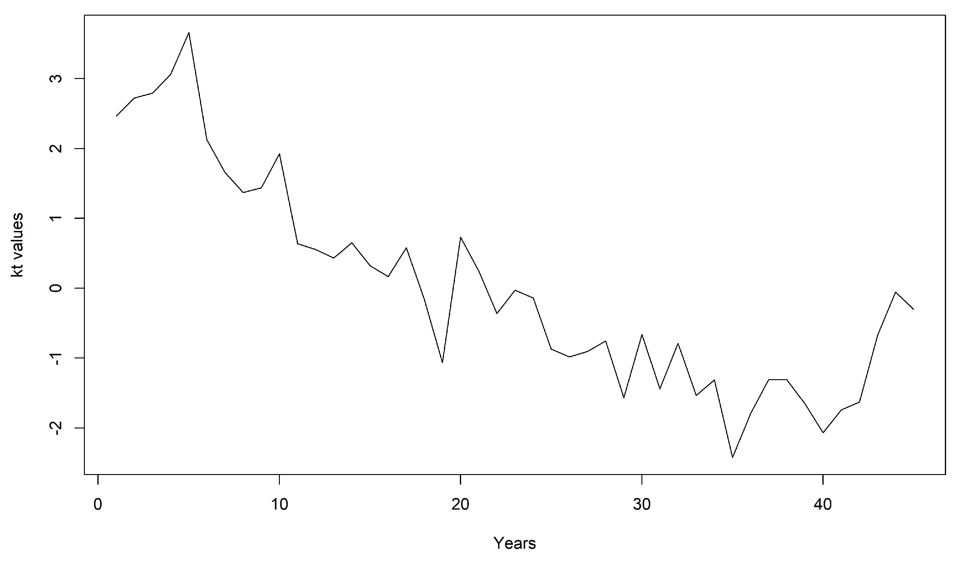
The estimated , , parameter values are shown in Table 2, while time-varying index is illustrated in Figure 1.

Table 2.
Estimated parameters for the U.K.
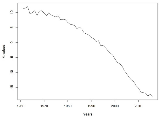
Figure 1.
Estimated values of .
Given the estimated parameters, the closed-form expression for the expected future central death rates can be derived as follows:
4.3. Modelling the Book Population
With the reference population in hand, it is now time to investigate the book population’s mortality dynamics. Estimating the reference population first allows us to make knowledgeable decisions regarding the model’s book part, and we can also incorporate features from the reference population (Villegas et al. 2017).
The dynamics of the book population’s mortality are specified through the log mortality differences of the book population and the reference population. In this paper, we compare the most commonly used models, which are the Lee–Carter model, the age-period-cohort (APC) model, the Cairns–Blake–Dowd (CBD) model, and the common age effect models to model the book population.
Note that for all the models being compared, we assume that .
4.3.1. The Lee–Carter Model
The dynamics of the book population are given as follows:
The term denotes the difference in the book population’s level of mortality compared to that of the reference population for age x. Thus, we can conclude that the mortality level in the book equals . Time index contributes to establishing the difference that exists in the mortality trends. The term shows us how differences in mortality for age x will respond if any change occurs in time index (Haberman et al. 2014).
4.3.2. The Common Age Effect Model
This model may be seen as an extension of the Lee–Carter model that possesses a common age effect. It can be given by the following equation:
The and parameters here are the same as in the LC model for the book population. Different from the LC model, there is a common age effect parameter, , which is the same as for the reference model.
4.3.3. The APC Model
The APC model was introduced by Currie (2006), and it is widely used in the literature. It can be regarded as a generalisation of the LC model, and a two-population version of this model may be written in the following way:
, and respectively represent the age, period, and cohort effects of the book population Currie (2006). The term is utilized here in order to account for differences that exist in the cohort effect in the two populations of interest. These parameters reflect the mortality differences between the two populations.
4.3.4. The CBD Model
Cairns et al. (2006) introduced the following model with the aim of fitting the mortality rates:
and are two stochastic processes and represent the time indices of the book population. These parameters reflect the mortality differences between the two populations as in the APC model.
The analysis of the models considered in this section becomes something of a challenge due to the CBD model directly modelling one-year death rate , while the others that are being considered in the paper model central death rates . In order to compare the models in a consistent way, we must introduce an additional step for the modelling of . We transform the one-year death probabilities in the central death rates using the identity . For all mentioned models, the parameters are estimated by two main steps. As indicated before, the parameters of the book population are estimated conditional on the parameters of the reference population. Under the Poisson assumption, the log-likelihood function of the book population is as follows:
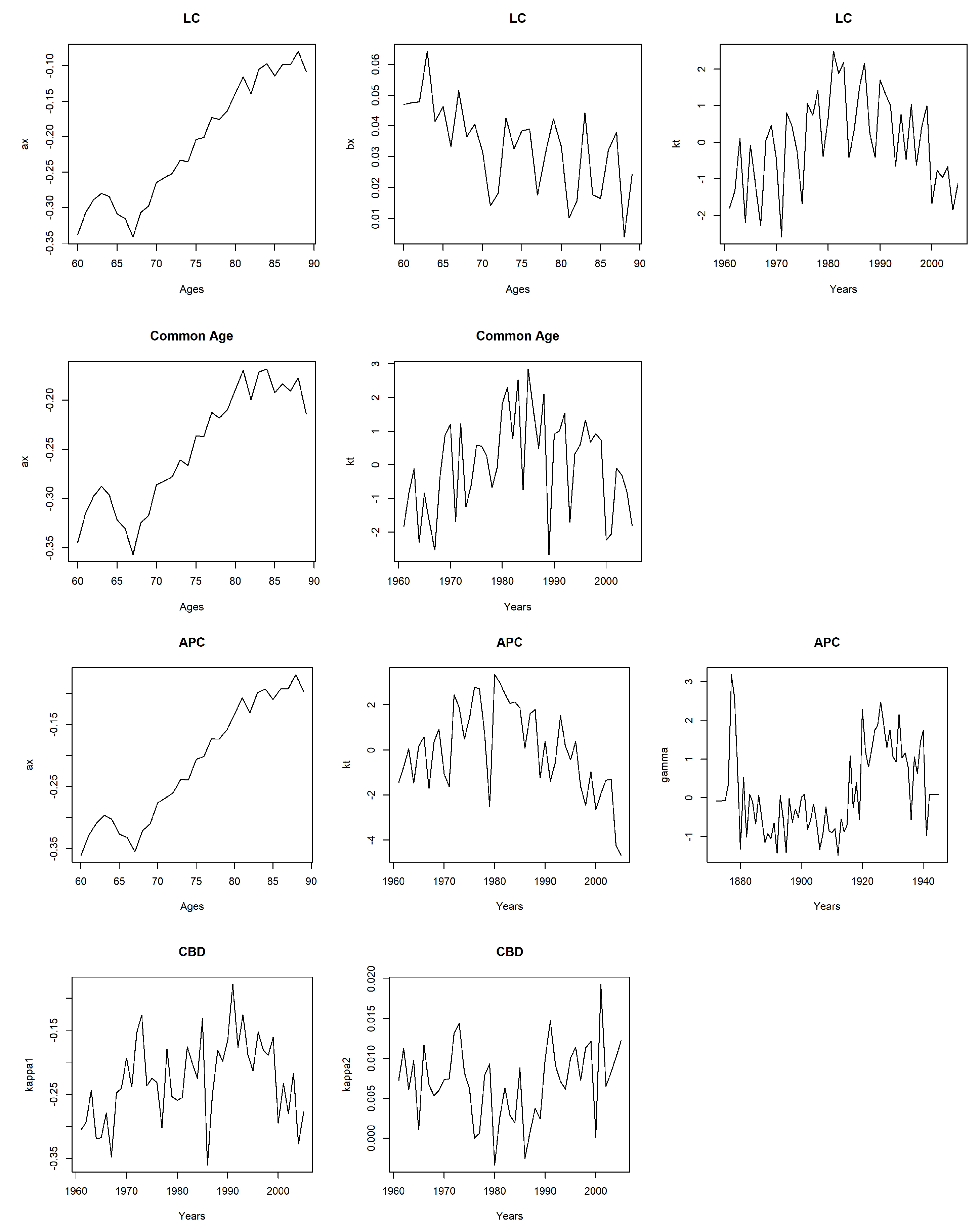
We estimate the parameters by applying the maximum likelihood method. The parameters obtained for the book population are given in Figure 2 for different mortality models.
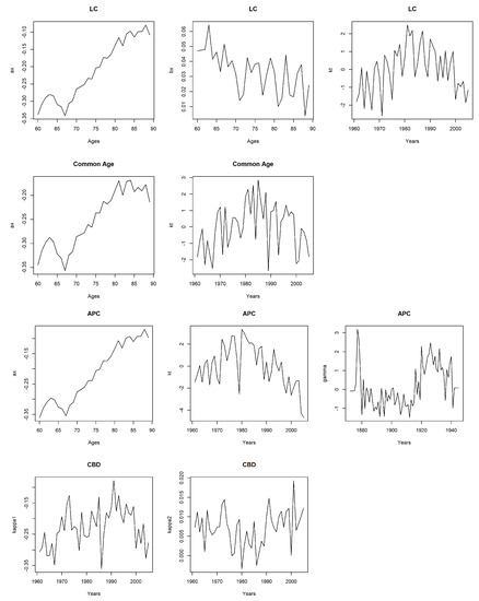
Figure 2.
Estimated parameters of the book population models.
According to Figure 2, the parameter shows that the younger ages reveal lower rates of mortality while the older ages reveal higher mortality. The positive values of demonstrate that mortality decreases for all ages. These results are valid for all and parameters for all mortality models of the book population. The mortality index, , reflects the changes in mortality rates over the years for the LC, common age, and APC models. The parameter represents the cohort related effects in the book population. The negative values of the parameter in the CBD model indicate the lower mortality rates, while the positive values reflect the higher mortality rates. The parameter controls these lower and higher mortality rates in the CBD model for the book population.
The BIC values obtained from the fitted models for book population mortality are given in Table 3. The common age effect model has the lowest BIC value according to Table 3. Therefore, we model the book population’s mortality using the common age effect model.

Table 3.
BIC Values for the Book Population Models.
Finally, we complete the modelling framework by specifying the period’s dynamics and the cohort terms, which will be used to forecast and simulate the future rates of mortality. A detailed analysis regarding the selection of the time series to be used in the dynamics can be found in the work of Li et al. (2015). This part of the study confines itself to focusing on the models that are commonly applied in the literature. We assume that the two populations will experience similar improvements in the long run, and thus, we assume that the spread in both time indices and cohort effects should be modelled as a stationary process.
In this paper, the time-varying mortality indices of the book population are modelled as an autoregressive process of order one; we are thus able to write for the LC, the common age effect, and the APC models. In the long term, the mean of equals if . The autocorrelation depends on the size of . More technical aspects of time-series modelling can be found in the work of Tsay (2002).
4.4. Future Simulations
In evaluating the uncertainty of future outcomes and finding the optimal model to assess longevity basis risk, it is necessary to address all of the parameter errors, process errors, and model errors from a modelling or a regulatory perspective such as that of Solvency II (Li et al. 2018). Parameter error refers to the uncertainty in estimating model parameters, while process error arises from variations that exist within the time series. Finally, model error reflects the uncertainty that is present in the model selection.
In the literature, a number of studies have been proposed to allow for both process error and parameter error in index-based hedging. For instance, Brouhns et al. (2002) used a parametric Monte Carlo simulation method for the generation of examples of model parameters following a multivariate normal distribution. Later, in a subsequent work, Brouhns et al. (2005) also explored a semi-parametric bootstrapping procedure designed for the simulation of death rates from the Poisson distribution with the obtained mean equalling the observed number of deaths. On the other hand, Renshaw and Haberman (2008) utilized the fitted number of deaths by using the Poisson process. In another study, Koissi et al. (2006) used a bootstrap method for the residuals of a fitted Lee–Carter model.
Different from the existing methods, Czado et al. (2005) and Kogure et al. (2009) suggested the application of Bayesian adaptations of the LC model. Li (2014) quantitatively compared possible methods for simulations; according to the conclusions of that study, sampling results will all be relatively close to each other regardless of whether the method applied is parametric, semi-parametric, Bayesian, or residual bootstrapping. All of these various simulation methods possess individual advantages and disadvantages. In this study, the bootstrapping method of Brouhns et al. (2005) was selected due to its ability to helpfully include both parameter errors and process errors in simulating future mortality rates. The procedure of bootstrapping is given below:
- The parameters of the LC model are estimated by using original data. Once they are obtained, those estimated parameters are then applied for estimating the number of deaths for both the reference and the book population by , .
- The new data on the number of deaths are simulated from a binomial distribution for the book population to include sampling risk, and the Poisson distribution is used for the reference population. The newly simulated data will then be used for the estimation of the reference and book populations’ mortality parameters. Incorporating this step means that the model can allow for parameter error.
- Next, we must fit time-series processes to the new data sample’s temporal model parameters, and , since we want to be able to simulate their future values. Furthermore, the inclusion of this step means that the model can allow for process error. is modelled by using the proposed model, and is modelled by using AR(1).
- We generate future mortality rate samples for all x and future t with the incorporation of the parameters obtained in Step (2) and the simulated values that we gained in Step (3) into and . As a result, our set of future mortality rates will form one random future scenario.
- We repeat Steps (1) to (4) until we have produced a total of 10,000 random future scenarios.
Different from Haberman et al. (2014), in this paper, the parameter errors of the reference population are considered by applying bootstrapping to both the reference and book population models’ estimations.
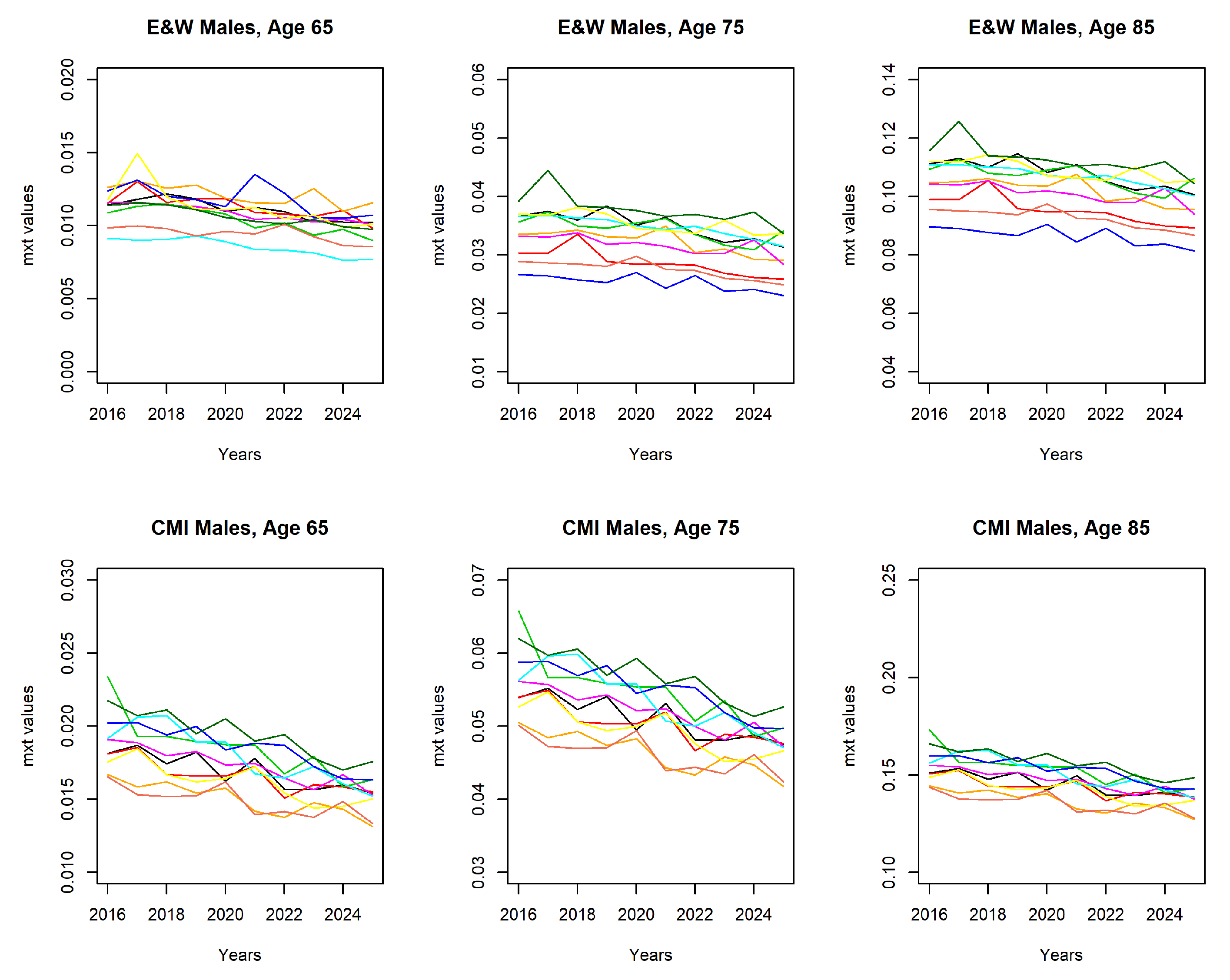
A sample from the simulated mortality paths are shown in Figure 3. The mortality paths enable us to obtain projected mortality rates, hence future liabilities of the pension plan and hedging instrument.
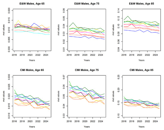
Figure 3.
Sample paths of . CMI, Continuous Mortality Investigation.
Sampling Risk
Sampling risk arises from the finite sizes of the reference and book populations and random outcomes of the individual lives. If the size of the populations are infinite, the future outcomes will converge the true expected values according to the law of large numbers. Nevertheless, the size of the populations is limited in reality. Although the bigger countries have very large population sizes, the annuity or pension portfolio’s size is usually small. Hence, the book and reference populations’ outcomes will deviate randomly from their true expected values, as well as from each other. To reflect the effect of the portfolio size, the number of lives is simulated as:
is the future number of lives aged x at time t of the book population. is the future mortality rate at age x at time t, and it is simulated from the semi-parametric bootstrapping method. Simulating the number of lives of the book population by using the binomial distribution provides protection from sampling risk (Li et al. 2018).
4.5. Comparison with the Other Mortality Models
After constructing a two-population mortality model, we need to compare the proposed model with other mortality models and show its effectiveness. Therefore, we consider three additional two-population mortality models. The first model is the LC model with normal jumps and the renewal process; the second one is the LC model with jumps; and the last one is the LC with common age effect model called CAE + Cohorts. The LC model with normal jumps and the renewal process has the same properties as the proposed mortality model. The only difference is the distribution of the mortality jumps. The model is expressed as:
where .
The LC with jumps model is very similar to Zhou et al. (2013); however, we use the relative approach to estimate the parameters of the models. Thus, our mortality data could be based on different sizes of periods for the reference and book population. As mentioned in Section 4.3, in the relative approach, the parameters of the reference population’s mortality model are estimated first. Then, the dynamics of the book population’s mortality are specified through the log mortality differences of the book population and the reference population. We use the same notation as Zhou et al. (2013) for the LC model with jumps, and the model is as follows:
where and are the same as in the original LC model. The time index is expressed as the sum of two components, . The first component, , is the time-t value of an unobserved period effect index that is free of jumps, while the second term, , indicates the jump effect at time t. The model allows the two populations to have different jump times, jump frequencies, and jump severities. They allow a maximum of one jump in a given year, and the jump severity follows a normal distribution with mean and variance (see Zhou et al. (2013) for more model details).
The last mortality model that we consider here is the CAE + Cohorts model that is given in Section 3. The parameters of the models are estimated by using the maximum likelihood method.
The estimated parameters for these three models are given in Appendix A.
5. Assessing Basis Risk: An Example
In this section, we consider a hedging strategy to assess longevity basis risk and to measure the effectiveness of the hedge while taking mortality jumps and sampling risk into account. The hedge effectiveness can be described as how much longevity risk is transferred away. The following formula can be used to define the level of longevity risk reduction for the hedge as in Coughlan et al. (2011):
where the terms risk (unhedged) and risk (hedged) represent the appropriate dispersion-based risk measures for the aggregate longevity of the portfolio before and after the hedging. A perfect hedge would have a longevity risk reduction equal to one, and a good hedge would have a risk reduction degree close to one; a risk reduction degree close to zero indicates an ineffective hedge (Dowd et al. 2019). In this paper, the variance risk measure is used to minimise the variations in the expected future cash flows of the hedging instrument.
A simple case study based on a hypothetical pension plan is considered to illustrate the effect of the proposed mortality models and different volumes of book population data on hedge effectiveness. The pension plan members are assumed to have underlying mortality rates that are the same as the CMI male assured lives dataset. Suppose that all members of the pension plan are aged 65 and pay £1 per year on survival from ages 66 to 90. Our objective is to minimise the longevity risk exposure of the pension plan, and hence, we construct a hedge by using a 10 year index-based longevity swap. We assume that the EW male population constitutes the floating leg’s reference population, while the payments of the fixed leg of the swap calculated by using Equation (20) are based on the CMI assured male lives. We assume that the interest rate is 3% per annum during the whole period. The current date is taken as the start of the calendar year 2016.
We use the same notation as in the work of Li et al. (2018) for the hedged and the unhedged positions. The present value of the pension plan’s future liability (unhedged position), , is given as below:
As a floating-leg receiver, the present value of the longevity swap’s future cash inflows, , can be written as:
For this equation, we calculate random future survivor index and forward survivor index by applying the survival probability formula, as follows: . Furthermore, the present value of the aggregate pension plan position after longevity hedging (hedged position) may be expressed with the following statement:
where weight w denotes the notional amount of longevity swap necessary for successful hedging to be performed. It is estimated by minimising the risk or uncertainty of the random present value of the aggregate position (Li et al. 2018).
Moreover, in order to take sampling risk into account, we use the binomial death process for the book population as given in Equation (14). To emphasise the role of the size of the population on hedge effectiveness, we produce three simulated distributions as , 10,000, and 100,000. We obtain cash flows for hedged and unhedged positions for four mortality models, namely the proposed Lee–Carter model with the renewal process and exponential jumps, the Lee–Carter model with the renewal process and normal jumps, and the LC model with jumps and CAE + Cohorts, by considering sampling risk. Then, the hedge effectiveness of these models is calculated.
In Table 4, we present the longevity risk reduction levels when sampling risk is taken into account for the three mortality models. The results indicate that our proposed mortality jump model with the renewal process provides a better risk reduction compared to the other two models. The risk reduction level increases as the sample size increases for all models, which indicates that sampling risk might be important. However, even for the smaller populations, our proposed model provides a 45.07% risk reduction, while the Lee–Carter model with the renewal process and normal jumps, the LC model with jumps, and the CAE + Cohorts model provide 33.97%, 23.17%, and 13.35%, respectively. Moreover, the mortality models with the renewal process show more risk reduction compared to the other mortality models. Therefore, the analysis shows that, by using the proposed mortality model, a significant portion of the risk would be eliminated for the pension plan that is exposed to mortality jump risk.

Table 4.
Risk reduction for different mortality models.
6. Conclusions
Index-based hedging solutions have many advantages. In such capital market solutions, it is possible to transfer the longevity risk to capital markets at lower costs. However, the potential differences between hedging instruments and the pension or annuity portfolio cause longevity basis risk. In this paper, we construct a two-population mortality model to measure and manage longevity basis risk.
An appropriate two-population model was built for EW male lives and CMI assured male lives to measure longevity basis risk, and the relative approach to model the populations was adopted. The modelling process of the reference population was followed by the modelling of the dynamics of the book population’s mortality. The reference population was modelled by using the LC model with renewal process and exponential jumps proposed by Özen and Şahin (2020), and the common age effect model outperformed among the others to model the book population.
The bootstrap approach of Brouhns et al. (2005) was applied in order to include both parameter error and process error in the simulation of future mortality rates. The Poisson distribution was used for the simulation of the reference population’s lives, and the binomial distribution was used for the simulation of the book population’s lives to consider sampling risk.
Furthermore, the impact of the proposed mortality model and sampling risk to hedge effectiveness was examined. For this purpose, a hypothetical pension plan and hedging strategy which consisted of a 10 year longevity swap were considered based on the three different two-population mortality models, namely the proposed LC model with the renewal process and exponential jumps, the LC model with the renewal process and normal jumps, the LC with jumps model, and the LC with common age effect model. Then, the hedge effectiveness was calculated by using these four mortality models to compare the risk reduction caused by the models. The analysis suggests that the proposed mortality model provides a more effective risk reduction for mortality jump risk and sampling risk than the other three models.
In this paper, the index-based longevity swaps were used as a hedging instrument to assess the longevity risk reduction. However, as a future study, a different hedging instrument such as q-forwards might also be included in the analyses to provide a more robust assessment of the basis risk. Another possible future study can be to construct an optimal hedging framework with collateralisation to obtain reasonable risk reduction rates by using the proposed two-population model.
Author Contributions
Conceptualization, S.Ö. and Ş.Ş.; methodology, S.Ö. and Ş.Ş.; software, S.Ö.; validation, S.Ö. and Ş.Ş.; formal analysis, S.Ö. and Ş.Ş.; investigation, S.Ö. and Ş.Ş.; resources, S.Ö. and Ş.Ş.; data curation, S.Ö. and Ş.Ş.; writing—original draft preparation, S.Ö. and Ş.Ş.; writing—review and editing, Ş.Ş.; visualization, S.Ö. and Ş.Ş.; supervision, Ş.Ş. All authors read and agreed to the published version of the manuscript.
Funding
This research received no external funding.
Institutional Review Board Statement
Not applicable.
Informed Consent Statement
Not applicable.
Data Availability Statement
https://www.mortality.org/ (4 January 2021) and Continuous Mortality Investigation Reports.
Conflicts of Interest
The authors declare no conflict of interest.
Appendix A
In this section, the parameters of the LC model with the renewal process and normal jumps, the LC model with jumps, and CAE + Cohorts are presented.
The and parameters are the same for all models.
The jump-diffusion parameters for the LC model with the renewal process and normal jumps are presented in Table A1.

Table A1.
Estimated jump-diffusion parameters.
Table A1.
Estimated jump-diffusion parameters.
| Jump Diffusion Parameters | ||||||
|---|---|---|---|---|---|---|
| 0.2389 | 0.1788 | 0.0355 | 0.3640 | 0.0029 | 0.6009 | |
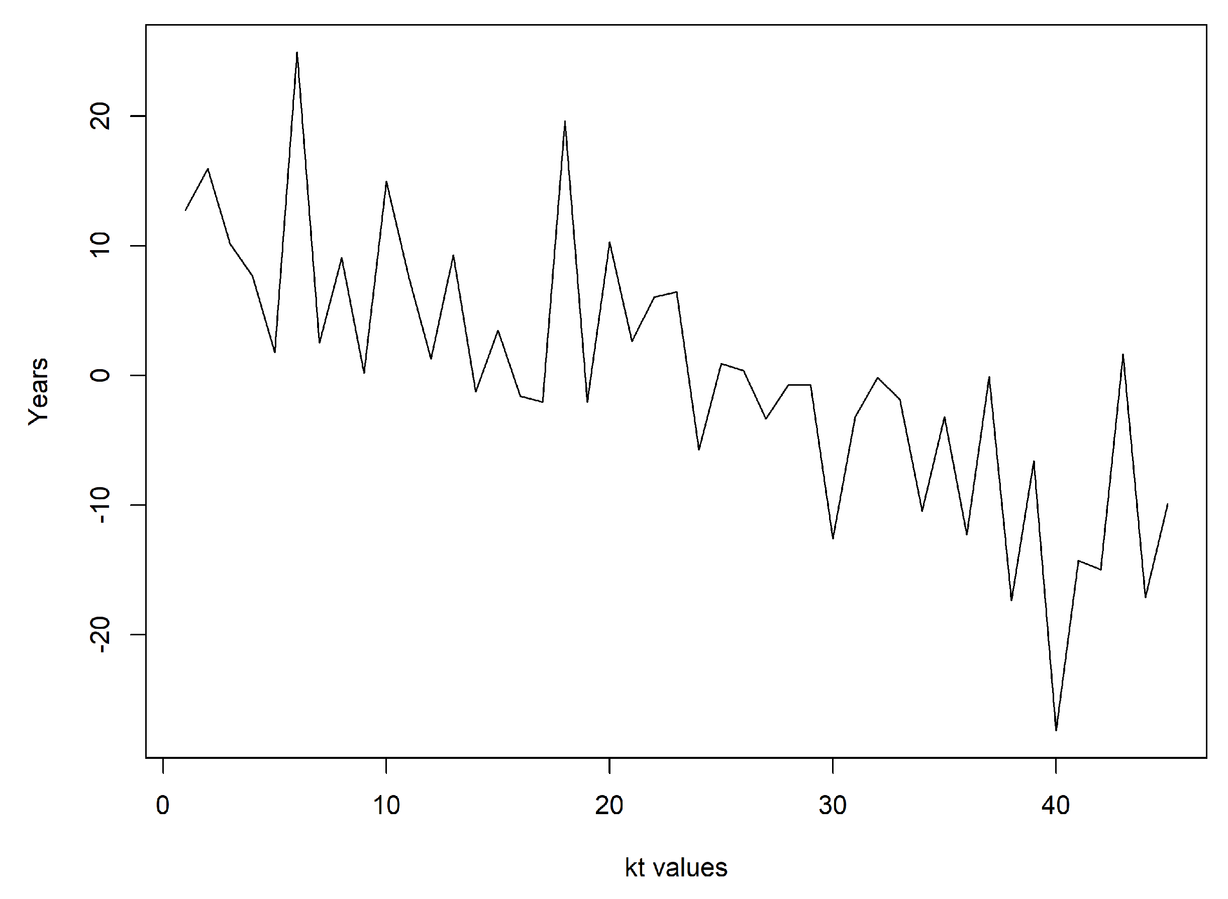
The estimated values are the same as the proposed model. The estimated and parameters are given in Table A2 and Figure A1.

Table A2.
Estimated book population parameters for the LC with the renewal process and normal jumps.
Table A2.
Estimated book population parameters for the LC with the renewal process and normal jumps.
| Age | Age | ||
|---|---|---|---|
| 60 | −1.1472 | 75 | −0.8633 |
| 61 | −1.1124 | 76 | −0.8462 |
| 62 | −1.1094 | 77 | −0.7794 |
| 63 | −1.1052 | 78 | −0.7739 |
| 64 | −1.1142 | 79 | −0.7382 |
| 65 | −1.1226 | 80 | −0.6980 |
| 66 | −1.1048 | 81 | −0.6433 |
| 67 | −1.1324 | 82 | −0.6805 |
| 68 | −1.0858 | 83 | −0.6239 |
| 69 | −1.0674 | 84 | −0.6235 |
| 70 | −1.0107 | 85 | −0.6215 |
| 71 | −0.9566 | 86 | −0.6155 |
| 72 | −0.9685 | 87 | −0.5836 |
| 73 | −0.9341 | 88 | −0.5391 |
| 74 | −0.9186 | 89 | −0.5532 |
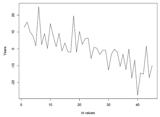
Figure A1.
Estimated values of the book population.
Figure A1.
Estimated values of the book population.
In Zhou et al. (2013), followed a random walk with drift, and followed a stationary first order autoregressive process. The period effect indices are modelled using by the following set of equations:
where and are constants and is a constant whose absolute value is less than one. The error terms and follow a zero-mean bivariate normal distribution with a variance-covarinace matrix .
The estimated and parameters are given in Table A3.

Table A3.
Estimated parameters for the LC with jumps model.
Table A3.
Estimated parameters for the LC with jumps model.
| Age | Age | ||||
|---|---|---|---|---|---|
| 60 | −0.8348 | 0.0234 | 75 | −0.6154 | 0.0188 |
| 61 | −0.8006 | 0.0230 | 76 | −0.6021 | 0.0166 |
| 62 | −0.7823 | 0.0217 | 77 | −0.5548 | 0.0167 |
| 63 | −0.7775 | 0.0222 | 78 | −0.5528 | 0.0159 |
| 64 | −0.7879 | 0.0225 | 79 | −0.5282 | 0.0146 |
| 65 | −0.8082 | 0.0234 | 80 | −0.4969 | 0.0153 |
| 66 | −0.7920 | 0.0205 | 81 | −0.4566 | 0.0136 |
| 67 | −0.8199 | 0.0199 | 82 | −0.4905 | 0.0126 |
| 68 | −0.7798 | 0.0199 | 83 | −0.4426 | 0.0131 |
| 69 | −0.7650 | 0.0194 | 84 | −0.4414 | 0.0124 |
| 70 | −0.7193 | 0.0189 | 85 | −0.4493 | 0.0124 |
| 71 | −0.6876 | 0.0177 | 86 | −0.4449 | 0.0140 |
| 72 | −0.6941 | 0.0191 | 87 | −0.4244 | 0.0131 |
| 73 | −0.6655 | 0.0175 | 88 | −0.3931 | 0.0106 |
| 74 | −0.6572 | 0.0168 | 89 | −0.4136 | 0.0113 |
The parameters of the jump component of the model are presented in Table A4.

Table A4.
Estimated parameters for the LC with jumps model.
Table A4.
Estimated parameters for the LC with jumps model.
The probabilities of jump frequencies are , , and .

Table A5.
Estimated parameters for the book population of the CAE + Cohorts model.
Table A5.
Estimated parameters for the book population of the CAE + Cohorts model.
| Age | Age | ||
|---|---|---|---|
| 60 | −0.5431 | 75 | −0.3930 |
| 61 | −0.5123 | 76 | −0.3886 |
| 62 | −0.4981 | 77 | −0.3545 |
| 63 | −0.4897 | 78 | −0.3569 |
| 64 | −0.4995 | 79 | −0.3419 |
| 65 | −0.5207 | 80 | −0.3171 |
| 66 | −0.5223 | 81 | −0.2893 |
| 67 | −0.5495 | 82 | −0.3201 |
| 68 | −0.5135 | 83 | −0.2828 |
| 69 | −0.5032 | 84 | −0.2801 |
| 70 | −0.4664 | 85 | −0.2988 |
| 71 | −0.4513 | 86 | −0.2904 |
| 72 | −0.4500 | 87 | −0.2846 |
| 73 | −0.4293 | 88 | −0.2639 |
| 74 | −0.4287 | 89 | −0.2944 |
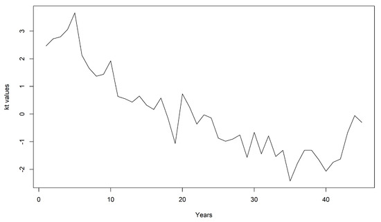
Figure A2.
Estimated values of the book population.
Figure A2.
Estimated values of the book population.
References
- Ahmadi, Seyed S., and Johnny Siu-Hang Li. 2014. Coherent Mortality Forecasting with Generalized Linear Models: A Modified Time-Transformation Approach. Insurance: Mathematics and Economics 59: 149–221. [Google Scholar] [CrossRef]
- Biatat, Viani D., and Iain D. Currie. 2010. Joint Models for Classification and Comparison of Mortality in Different Countries. Paper Presented at 25rd International Workshop on Statistical Modelling, Glasgow, Scotland, July 4–9. [Google Scholar]
- Brouhns, Natacha, Michel Denuit, and Ingrid Van Keilegom. 2005. Bootstrapping the Poisson log-bilinear Model for Mortality Forecasting. Scandinavian Actuarial Journal 31: 212–24. [Google Scholar] [CrossRef]
- Brouhns, Natacha, Micheal Denuit, and Jeroen K. Vermunt. 2002. Measuring the Longevity Risk in Mortality Projections. Bulletin of Swiss Association, 105–30. [Google Scholar] [CrossRef]
- Cairns, Andrew J. G., David Blake, and Kevin Dowd. 2006. A Two-Factor Model for Stochastic Mortality with Parameter Uncertainty: Theory and Calibration. Journal of Risk and Insurance 73: 687–718. [Google Scholar] [CrossRef]
- Cairns, Andrew J. G., David Blake, Kevin Dowd, and Guy D. Coughlan. 2011. Bayesian Stochastic Mortality Modelling for Two Populations. ASTIN Bulletin 41: 29–59. [Google Scholar]
- Cairns, Andrew J. G., David Blake, Kevin Dowd, and Guy D. Coughlan. 2014. Longevity Hedge Effectiveness: A Decomposition. Quantitative Finance 14: 217–35. [Google Scholar] [CrossRef]
- Carter, Lawrence R., and Ronald D. Lee. 1992. Modeling and Forecasting US Sex Differentials in Mortality. International Journal of Forecasting 8: 393–411. [Google Scholar] [CrossRef]
- Chen, Hua, and Samuel H. Cox. 2009. Modeling Mortality with Jumps: Applications to Mortality Securitization. The Journal of Risk and Insurance 76: 727–51. [Google Scholar] [CrossRef]
- Coughlan, Guy D., Marva Khalaf-Allah, Yijing Ye, Sumit Kumar, Andrew J. G. Cairns, David Blake, and Kevin Dowd. 2011. Longevity Hedging 101: A Framework for Longevity Basis Risk Analysis and Hedge Effectiveness. North American Actuarial Journal 15: 150–76. [Google Scholar] [CrossRef]
- Currie, Iain D. 2006. Smoothing and Forecasting Mortality Rates with P-splines. Statistical Modelling 4. [Google Scholar] [CrossRef]
- Czado, Claudia, Antoine Delwarde, and Micheal Denuit. 2005. Bayesian Poisson log-bilinear Mortality Projections. Insurance: Mathematics and Economics 36: 260–84. [Google Scholar] [CrossRef]
- Dowd, Kevin, Andrew J. G. Cairns, and David Blake. 2019. Hedging Annuity Riskswith the Age-Period-Cohort Two-Population Gravity Model. North American Actuarial Journal, 1–12. [Google Scholar] [CrossRef]
- Dowd, Kevin, David Blake, Andrew J. G. Cairns, and Guy D. Coughlan. 2011. Hedging Pension Risks with the Age-Period-Cohort Two-Population Gravity Model. Paper Presented at the 7th International Longevity Risk and Capital Market Solutions Conference, Goethe University’s Campus Westend, Frankfurt, Germany, September 8–9. [Google Scholar]
- Haberman, Steven, Vladimir K. Kaishev, Pietro Millossovich, and Andres M. Villlegas. 2014. Longevity Basis Risk: A Methodology for Assessing Basis Risk. Research Report. London: Institute and Faculty of Actuaries, Life and Longevity Markets Association. [Google Scholar]
- Hatzopoulos, Petros, and Steven Haberman. 2013. Common Mortality Modeling and Coherent Forecasts: An Empirical Analysis of Worldwide Mortality Data. Insurance: Mathematics and Economics 52: 320–37. [Google Scholar] [CrossRef]
- Jarner, Soren F., and Esben Masotti Kryger. 2011. Modelling Adult Mortality in Small Populations: The SAINT Model. ASTIN Bulletin 41: 337–418. [Google Scholar]
- Koissi, Marie-Claire, Arnold F. Shapiro, and Göran Högnas. 2006. Evaluating and Extending the Lee–Carter Model for Mortality Forecasting: Bootstrap Confidence Interval. Insurance: Mathematics and Economics 38: 1–20. [Google Scholar] [CrossRef]
- Kogure, Atsuyuki, Kenji Kitsukawa, and Yoshiyuki Kurachi. 2009. A Bayesian Comparison of Models for Changing Mortality Towards Evaluating the Longevity Risk in Japan. Asia Pasific Journal of Risk and Insurance 3: 1–22. [Google Scholar] [CrossRef]
- Li, Hang, and Mary Hardy. 2011. Measuring Basis Risk in Longevity Hedges. North American Actuarial Journal 15: 177–200. [Google Scholar] [CrossRef]
- Li, Jackie. 2014. A Quantitative Comparison of Simulation Strategies for Mortality Projection. Annals of Actuarial Science 8: 281–97. [Google Scholar] [CrossRef]
- Li, Jackie, Johnny Siu-Hang Li, Chong It Tan, and Leonie Tickle. 2018. Assessing basis risk in index-based longevity swap transactions. Annals of Actuarial Science 13: 1–32. [Google Scholar] [CrossRef]
- Li, Nan, and Ronald Lee. 2005. Coherent Mortality Forecasts for a Group of Populations: An Extension of the Lee–Carter Model. Demography 42: 575–94. [Google Scholar] [CrossRef] [PubMed]
- Li, Johnny Siu-Hang, Rui Zhou, and Mary Hardy. 2015. A Step by Step Guide to Building Two Population Stochastic Mortality Models. Insurance: Mathematics and Economics 63: 121–34. [Google Scholar] [CrossRef]
- Ngai, Andrew, and Micheal Sherris. 2011. Longevity Risk Management for Life and Variable Annuities: The Effectiveness of Static Hedging Using Longevity Bonds and Derivatives. Insurance: Mathematics and Economics 49: 100–14. [Google Scholar] [CrossRef]
- Özen, Selin, and Şule Şahin. 2020. Transitory Mortality Jump Modeling with Renewal Process and Its Impact on Pricing of Catastrophic Bonds. Journal of Computational and Applied Mathematics 376: 1–15. [Google Scholar] [CrossRef]
- Renshaw, Arthur, and Steve Haberman. 2008. On Simulation Based Approaches to Risk Measurement in Mortality with Specific Reference to Poisson Lee–Carter Modelling. Insurance: Mathematics and Economics 42: 797–816. [Google Scholar] [CrossRef]
- Tsay, Rue S. 2002. Analysis of Financial Time Series. New York: John Wiley & Sons. [Google Scholar]
- Villegas, Andres M., Steven Haberman, Vladimir K. Kaishev, and Pietro Millossovich. 2017. A Comparative Study of Two-Population Models for the Assessment of Basis Risk in Longevity Hedges. ASTIN Bulletin 47: 631–79. [Google Scholar] [CrossRef]
- Zhou, Rui, Johnny Siu-Hang Li, and Ken Seng Tan. 2013. Pricing Standardized Mortality Securitizations: A Two-Population Model With Transitory Jump Effects. The Journal of Risk and Insurance 80: 733–74. [Google Scholar] [CrossRef]
- Zhou, Rui, Yujiao Wang, Kai Kaufhold, Johnny Siu-Hang Li, and Ken Seng Tan. 2014. Modeling Period Effects in Multi-Population Mortality Models: Applications to Solvency II. North American Actuarial Journal 18: 150–67. [Google Scholar] [CrossRef]
Publisher’s Note: MDPI stays neutral with regard to jurisdictional claims in published maps and institutional affiliations. |
© 2021 by the authors. Licensee MDPI, Basel, Switzerland. This article is an open access article distributed under the terms and conditions of the Creative Commons Attribution (CC BY) license (http://creativecommons.org/licenses/by/4.0/).


