Use of Neural Networks to Accommodate Seasonal Fluctuations When Equalizing Time Series for the CZK/RMB Exchange Rate

Abstract

The global nature of the Czech economy means that quantitative knowledge of the influence of the exchange rate provides useful information for all participants in the international economy. Systematic and academic research show that the issue of estimating the Czech crown/Chinese yuan exchange rate, with consideration for seasonal fluctuations, has yet to be dealt with in detail. The aim of this contribution is to present a methodology based on neural networks that takes into consideration seasonal fluctuations when equalizing time series by using the Czech crown and Chinese yuan as examples. The analysis was conducted using daily information on the Czech crown/Chinese yuan exchange rate over a period of more than nine years. This is the equivalent of 3303 data inputs. Statistica software, version 12 by Dell Inc. was used to process the input data and, subsequently, to generate multi-layer perceptron networks and radial basis function neural networks. Two versions of neural structures were produced for regression purposes, the second of which used seasonal fluctuations as a categorical variable–year, month, day of the month and week—when the value was measured. All the generated and retained networks had the ability to equalize the analyzed time series, although the second variant demonstrated higher efficiency. The results indicate that additional variables help the equalized time series to retain order and precision. Of further interest is the finding that multi-layer perceptron networks are more efficient than radial basis function neural networks.

1. Introduction

At the microeconomic level, securing exchange rates has a significant impact on the development of a company´s cost base, profits, and financial viability, whilst on the macroeconomic level, on a country´s balance of trade. Such consequences may be the result of the correct or incorrect use of exchange rates, which is an issue many managers or important politicians will find hard to avoid. In a global economy, despite the current geopolitical and health concerns, exchange rates have a significant impact, particularly on the currencies of small and medium-sized countries, both at the micro- and macroeconomic levels (Vochozka et al. 2020).

Many economists share the view that foreign trade provides the opportunity to expand a country’s potential level of consumption. As a result of this growing openness, the global economy is approaching its ideal production capacity curve. Based on the above, it can be argued that foreign trade is a factor that largely affects the stability of economies and economic growth. This is no different for the Czech Republic and the People’s Republic of China.

Probably the most important indicator in the international trade environment is the exchange rate, which not only reflects the imports and exports price, but also the currency value. There is no doubt that changeability of exchange rates has a serious impact on the decisions of all entities operating in the international market for goods and services. For this reason, it is essential to set it correctly (Machova and Marecek 2019).

At present, research is focused on the development of methods that are best able to predict exchange rates. Although the scientific literature provides numerous theories and approaches used to estimate exchange rate developments including the factors affecting them, it is very surprising that the issue of seasonal fluctuations in the Czech crown/Chinese yuan exchange rate have not been addressed using artificial intelligence (artificial neural networks).

A number of studies dealing with the topic exist. However, they compare the Chinese yuan with other currencies. Similarly, the Czech crown is compared with those currencies more closely associated with it. This study is therefore unique, with the importance thereof growing with the increasing volume of Chinese investment in the Czech Republic (Foreign Direct Investment 2018–2019) and the growth of the trade balance. The aim of this paper was to present a methodological foundation based on the use of neural networks that takes into consideration the seasonal fluctuations when equalizing time series by using the Czech crown and Chinese yuan as examples.

With regard to the structure of the contribution, the literature review is partially devoted to international trade as a whole, and goes on to describe the results of studies on exchange rates and the prediction thereof using artificial intelligence. The Materials and Methods section includes the calculations for the two sets of neural networks. The results of both experiments are subsequently presented. Furthermore, the discussion provides a comparison of the results of both experiments with each other and also with those of other studies. The paper is concluded with a brief summary of all the important information and puts forward suggestions for further research.

2. Literature Review

As previously mentioned, according to Vrbka et al. (2019), international trade is considered to be crucial for economic growth, the essence of which consists of the exchange of goods, services, and capital across national borders. Horak and Machova (2019) stated that, in contrast to trade at the domestic level, the implementation of this trade type is a very complex process. On the other hand, Bernard (2004) added that for most countries, international trade plays a key role and represents a significant share of gross domestic product. The author further stated that the existence of foreign trade goes back a very long way, but that its social, political, and economic importance has only grown in recent centuries. Nevertheless, this statement does not change the fact that international trade has always been given due attention and has always been considered as very important. Li et al. (2019) considered international trade as an essential contributor to regional economic development. The authors claimed that those regions experiencing rapid growth in international trade were also those regions developing the most rapidly, as far as the economy is concerned. The issue of exchange rates is also very often discussed in connection with international trade.

Vochozka et al. (2019) stated that the conventional approach to the worldwide economy was based on the fact that exchange rates are seen as the main factor influencing external trade. Since the Czech economy is very closely linked to external trade, a quantitative understanding of the impact of exchange rates on exports and/or imports represents an essential piece of information for all participants in the field. Hnat and Tlapa (2014) stated that the reasons for the decision by states to open themselves up for international trade differ, depending on the conditions and natural resources of the given country as well as on the differences in consumer habits and tastes.

Cheong et al. (2006) examined, for example, the dynamic relationships between exchange rate uncertainty, international trade, and price competitiveness using the United Kingdom as their example. Results based on the empirical analysis by means of vector autoregressive models (VAR) showed that shocks that stimulate exchange rate volatility have a negative influence on trade volumes and that this negative impact is stronger than the influence on trade price levels.

Budikova et al. (2010) stated that, like most other economic information, exchange rates have certain time dynamics (i.e., they are recorded in the form of time series). There are several possible ways to define time series. Sheikhan et al. (2013) provided a definition of the concept of time series and described them as a sequence of spatially and factually comparable observations that are organized in time. De Baets and Harvey (2018) had a simpler definition; they understood time series as sequences of values of variables arranged in an orderly manner, evenly spaced over time. León-Alvarez et al. (2016) defined time series analysis as a method employing the study of individuals or groups observed at successive moments. These moments represent a particular series of data points presented in chronological order. The author further added that the analysis of time series can also provide us with significant statistics and other essential data characteristics. It can be stated that, without a doubt, forecasting is one of the most important tasks of time series analysis. The reason for this is that with the help of time series prediction, based on previously monitored values, it is possible to predict values for the future. Mai et al. (2018) stated that the analysis and measurement of time series can also be employed primarily for predictions in the future. The author goes on to describe time series as the monitoring of certain data arranged on a time horizon from the past to the present. According to Vochozka and Vrbka (2019), time series provides crucial insights into the entire exchange rate development process. Prediction is considered the most important function of time analysis. The analysis of time series is a field in which neural networks are widely used. Horak (2019) saw their advantage in the fact that in terms of prediction, neural networks worked with big data, therefore guaranteeing a relatively high level of accuracy; neural networks, together with time series, can be used for solving complex problems and predictions. It is, of course, possible to use standard structural exchange rate models or autoregressive conditionally heteroscedasticity (ARCH) and generalized autoregressive conditionally heteroscedasticity (GARCH) models and mutations thereof. These models focus on the assumption of heteroscedasticity. In essence, they form a systematic framework for volatility modeling. Theoretically, they can be employed very successfully to measure the development of and predict the price of exchange rates that meet the above-stated assumptions, as evidenced by Petrica and Stancu (2017), Quaicoe et al. (2015), You and Liu (2020), and Smallwood (2019). However, neural networks are a very suitable alternative that produce very interesting results, and of which the potential has not yet been fully exploited. An artificial neural network is a topological arrangement of individual neurons in a structure with the help of oriented evaluated connections. Each network is therefore characterized by the type of neuron, their topological arrangement, and the strategy of adaptation during network training (Alonso-Monsalve et al. 2020). The great advantage of neural networks is their profitability, whereby the main advantage lies in the ability to learn and capture hidden, even strongly non-linear dependencies. Based on the learned experience, they then estimate a new result (Henriquez and Kristjanpoller 2019). They are able to work with inaccurate data and noise. The principle of neural networks has now been implemented in various fields of human activity and in some analytical and decision-making software products, producing very good results (Parot et al. 2019).

For example, Laily et al. (2018) compared ARCH and GARCH models with the Elman recurrent neural network (ERNN) when analyzing stock prices. They found that the most suitable model in this case was GARCH, which had the smallest mean squared error (MSE). Ortiz Arango (2017), in turn, used GARCH models and neural network differentials (RND) to predict the future prices of financial assets, specifically the future development of the price of a barrel of oil. He found that neural networks produce better results than the basic GARCH model and are therefore a reliable alternative method for time series analysis. Lu et al. (2016), who predicted the volatility of log-returns in the Chinese energy market using the GARCH model and neural networks, also confirm the better predictive ability of neural networks. Similarly, Arneric et al. (2014), who examined the development of the Croatia stock market (CROBEX) or Mohamed (2013) index price by comparing GARCH models and neural networks for modeling financial returns in the market in the Arab Republic of Egypt, confirmed the better predictive power of neural networks in relation to GARCH models. Due to the findings from these studies, neural networks will be applied in this contribution for exchange rate prediction.

The application of NN (neural networks) for predicting and trading the EUR/USD exchange rate is described by Dunis et al. (2011). Dhamija and Bhalla (2011) found that NNs can be effectively used for forecasting exchange rates and therefore also for business strategy proposals. Guresen et al. (2011) also argued that exchange rate forecasting is an important financial issue, one that is receiving an ever-increasing amount of attention. Over the last few years, a number of neural network models and hybrid models have been put forward to exceed traditional prediction results in an effort to surpass traditional linear and non-linear approaches. Guresen et al. (2011) assessed the effectiveness of neural network models, which are known to be dynamic and effective in financial market forecasting. The analyzed models were multi-layer perceptrons (MLP), dynamic artificial neural networks (DAN2), and hybrid neural networks that use generalized autoregressive conditional heteroscedasticity (GARCH) to extract new input variables.

Sindelarova (2012) also dealt with the application of artificial neural networks (ANN) for the prediction of economic time series. First, she focused on the revision of the basic existing ANN architectures for predicting time series and described their application in predicting the CZK/EUR exchange rate. She also presented a hybrid version of ANN, as did Bielecki et al. (2008), which was based on the same network strategy, but tried to increase the prediction accuracy. The results of the studies are comparisons of the hybrid approach and the accuracy of traditional ANN settings for the CZK/EUR or USD/PLN exchange rates. However, due to the many parameters to be empirically assessed, it is not easy to choose a suitable NN architecture for the prediction of the exchange rate. Researchers frequently do not consider the influence of the neural network parameters on its performance. Zhang and Hu (1998) examined the effect of the number of the input and hidden nodes and the size of the training sample on the performance in and outside the sample. For a detailed examination, the GBP/USD exchange rate (prediction) was used. It was discovered that NNs outclass linear models, especially in the case of a short prediction horizon. Yin and Chen (2016) suggested a method for the application of the exponential generalized autoregressive conditional heteroscedasticity-M (EGARCH-M) model in connection with the Elman NN for predicting the return rate of the USD/CNY exchange rate. The EGARCH-M model captured the volatility asymmetry, plus the correlation between the return, and this one was past volatility; Elman’s NN was used so that it corresponded with the non-linear character of the return rate. GBP/CNY and USD/CNY exchange rate predictions were carried out by Liu et al. (2011) using predictions by RBF neural networks and GARCH models. CNY rates can be considered as a financial TS (time series) characterized by a high non-linearity and a change of behavior over time (Cai et al. 2012). CNY has grown from a trading currency to an investment currency and currently has the potential to be a worldwide reserve currency. The development of CNY as an international currency might balance the USD dominated system and add to regional and international financial stability (Ma and Mccauley 2011; Zhang and Sato 2012).

Interestingly, the correlation between the exchange rate and stock market performance was approached by Tian and Ma (2010), who used the autoregressive distributed lag model—ARDL’s cointegration approach to examine the impact of financial liberalization on the relationship between the exchange rate and stock market performance in China. They found that there was a cointegration between the Shanghai stock index and the renminbi (RMB) against the US dollar and the Hong Kong dollar from 2005, the year in which the Chinese exchange regime became a flexible, managed floating system. The authors found that the exchange rate and the money supply affected the share price with a positive correlation. They also showed that the increase in the money supply had been largely due to the huge influx of “hot money” from other countries in recent years.

The prediction of exchange rate changes, their link to other macroeconomic phenomena and possible geopolitical impacts have been the subject of an extremely extensive volume of research. For example, Ilzetzki et al. (2019) dealt with exchange rate arrangements and restrictive measures in 194 countries. Ho and Karim (2012) examined the significant relationship between exchange rates, macroeconomic fundamentals, and international trade in a group of Asian countries from 1980 to 2009. According to them, international trade is essential for developing countries for investment purposes and to attract foreign exchange in this liberalized and globalized world. Regression analyses show that market size and the exchange rate play a very important role in promoting international trade. Population growth has significant negative effects on developed countries like Japan and Singapore, but has positive effects on the Philippines. In addition, inflation rates have a negative impact on the Philippines and India, while financial market developments are only marginally significant in overall trade between Singapore and India. The results of the study represent the strategic policy implications for developing and developed Asian countries with regard to the facilitation of international trade and boosting growth.

In this specific field, the first area of research was concerned with the correlation of exchange rates and inflation or business cycles (De Boer et al. 2020). Forbes et al. (2018) used vector autoregressive modelling to reveal the links between the exchange rate and inflation, and Nguyen and Sato (2020) used the same method to detect asymmetries in the Japanese yen. Using an autoregressive approach, Grabowski and Welfe (2020) identified four main determinants of the currency market: inflation, terms of trade, country-specific risks, and the state of the currency market. The correlation of exchange rates and consumer prices with a vector autoregressive model was then examined by Ha et al. (2020). Thee VAR and the ARDL (autoregressive distributed lag) models were used by Chiappini and Lahet (2020) to find the key factors for 24 emerging economies, thereby demonstrating China’s fundamental influence on the exchange rates of other Asian countries. The same method was used by Dogru et al. (2019) to analyze the effect of exchange rates on bilateral trade between the United States, Mexico, Canada, and the United Kingdom. Ponomareva et al. (2019) used time series regression for predicting the exchange rates of the US dollar, Japanese yen, British pound, and euro as well as the Australian and Canadian dollars. When using the baltic dry index to predict the exchange rates, Han et al. (2020) employed the method of time series. The use of other analytical methods is rather an exception. Behavioral equilibrium models used by Kharrat et al. (2020) are also relatively common as part of optimizing monetary investment strategies.

It is mainly these investment strategies and optimal security that represent the second important area of research. Maggiori et al. (2020) focused on global portfolios and pointed out the difference between companies in the United States and other countries where securities were usually subscribed in foreign currency. Opie and Riddiough (2020) presented a new method for dynamically hedging currency exposure in international equity and bond portfolios using time series. The time series prediction test was also the basis of the spot exchange rate model for 16 currencies according to Narayan et al. (2020).

Bahmani-Oskooee and Hegerty (2007) provided an insight into history and stated that the increase in exchange rate volatility since 1973 has had indeterminate effects on international export and import flows. Although it can be assumed that an increase in risk may lead to a decrease in economic activity, the theoretical literature provides justification for positive or insignificant effects. Similar results were found in empirical tests. While modeling techniques have evolved over time to incorporate new developments into econometric analysis, no single degree of exchange rate volatility has dominated in the literature.

New patterns in intraday currency trading were revealed by Khademalomoom and Narayan (2020); and a currency trading strategy that took into account the predictive power of currency implied volatility was presented by Ornelas and Mauad (2019) and Accominotti et al. (2019).

Bulut (2018) successfully used Google Trends to predict exchange rates. Amo Baffour et al. (2019) dealt with the integration of an asymmetric model into an artificial neural network for the prediction of the exchange rates of five currencies. According to them, this hybrid solution dramatically increased the quality of the model.

The significant risk of generalization in the search for suitable predictive models was pointed out by Cheung et al. (2019). According to their research, the performance of models varied fundamentally, depending on the length of the prediction.

The effect of influencing the exchange rate in relation to the return on equity within the optimization models was revealed by Turkington and Yazdani (2020). An important topic is also investment in so-called safe-haven currencies, where, for example, Cho et al. (2020) are reducing the importance of the euro, which, according to them, is still one of the currencies that moves in opposition to global stock markets. The treasury-EuroDollar (TED) spread, and country-specific volatility and low liquidity factors were revealed by Maurer et al. (2019) as the two key sources of risk in foreign exchange (FX) markets.

Another area is represented by the use of exchange rates as an indicator of the state of an economy. Augustin et al. (2020) used currency swap spreads for this purpose, and Dahlquist and Hasseltoft (2020) stated the need to include inflation and economic stability in monetary trading strategies. Another important topic is the interconnectedness of exchange rates and commodity prices (Liu et al. 2020). The link between the type of commodities and the exchange rate, or their collapse, was revealed by Bodart and Carpantier (2020), according to whom the impact on agricultural exports was significantly greater compared to the relatively small impact on energy and/or mineral exports. The impact of oil price shocks, especially in the long run, on exchange rates was identified by Huang et al. (2020). Chernov et al. (2018) dealt with the quantification of the risk of currency shocks through an empirical model of bilateral exchange rates. Colacito et al. (2018) also focused on the 10 most traded currencies in the world. They stated their heterogeneity of exposure to trade and currency shocks. A separate chapter of the research concerns the assessment of the effectiveness of monetary unions (Groll and Monacelli 2020), very often with an overlap to crises such as that in Greece (Kriwoluzky et al. 2019). Chari et al. (2020) addressed the performance of economies and the benefits of a single currency. Bonadio et al. (2020) focused on the speed of the impact of an exchange rate shock in Switzerland. Furthermore, the topic of interventions in exchange rates in order to support export potential due to events in global markets is also current. However, as Rajković et al. (2020) showed in the example of the currencies of the Balkans and Central and Eastern Europe, currency depreciation did not have a significant effect on the trade deficit. Interestingly, Xing (2018) found the complete opposite to be true, with rising wages and the cumulative appreciation of the RMB undermining China’s comparative advantage. This was also confirmed by Choi and Choi (2018), who found that the devaluation of the RMB had a direct effect on reducing unemployment. Min and Yang (2019) looked at the problem of debt risks in a currency other than the domestic currency in South Korean companies.

With regard to the RMB, attention must also be paid to the impact of exchange rate changes on economic growth and income distribution. Ribeiro et al. (2020) stated that although low exchange rates lead to increased exports, they have a negative impact on the income of selected groups of the population. In a sample of 2500 pairs, Gopinath et al. (2020) primarily assessed the effect of exchange rates on business elasticity and determined the monetary paradigm. Research on the RMB is extensive, partly as a result of a series of analyses of the impact of the reform of the People’s Bank of China, which, according to Wen and Wang (2020), has led to reduced exchange rate volatility. This significant change was also addressed by Smallwood (2019), according to whom, exchange rate uncertainty has no effect on trade with the United States, or Cheung et al. (2018), who dealt with the impact of these changes on central parity. Liu and Woo (2018) also extensively analyzed the effects of the so-called trade war between these great powers, drawing attention to the rather vague term “equilibrium exchange rate” used by many politicians and economists.

Ho (2020) pointed out the strong effects of virtual currencies and their exchange rates, even in terms of inflation and economic growth for Taiwan and China.

3. Materials and Methods

The data for the analysis are accessible on the World Bank (2020) website. The information on the mutual exchange rates of the Czech crown (hereinafter referred to as “CZK”) and the Chinese yuan (hereinafter referred to as “RMB”) were used for the purpose of the analysis (i.e., the daily exchange rate records of these currencies). The time period began on 6 October 2009 and closed on 21 October 2018, which was the equivalent of 3303 data inputs. The unit was several CZK to one RMB.

The descriptive characteristics of the dataset are presented in

Table 1. Characteristics of the dataset.

Statistics	Date–Input Variable	RMB to CZK–Output (Aim)
Minimum (training)	40,092.00	2.485800
Maximum (training)	43,394.00	4.163000
Diameter (training)	41,734.79	3.265645
Standard deviation (training)	939.26	0.392383
Minimum (testing)	40,102.00	2.496100
Maximum (testing)	43,393.00	4.155700
Diameter (testing)	41,755.71	3.272882
Standard deviation (testing)	957.97	0.394309
Minimum (validation)	40,111.00	2.498900
Maximum (validation)	43,388.00	4.152900
Diameter (validation)	41,768.68	3.246446
Standard deviation (validation)	1,438.25	0.499822
Minimum (overall)	40,092.00	2.485800
Maximum (overall)	43,394.00	4.163000
Diameter (overall)	41,743.00	3.263852
Standard deviation (overall)	953.64	0.392668

Source: Own research.

.

Statistica software, version 12, by Dell Inc. was used for the data processing. Data mining, neural networks (i.e., automated neural networks (ANS)) were utilized for the computation of the neural structures. A regression was performed using neural structures. Multi-layer perceptron networks (MLP) and radial basis function (RBF) NNs were then generated. The MLP network has one or more hidden layers between the input and output layers, with the neurons arranged in layers, the connections always routed from the lower to higher layers, and with no interconnection between neurons in the same layer (see Figure 1) (Ramchoun et al. 2017).

The RBF network in its simplest form is a three-layer forward neural network. The first layer corresponds to the inputs to the network, the second layer is a hidden layer consisting of a series of non-linear activation RBF units, and the last layer corresponds to the final output of the network. Activation functions in RBF are conventionally implemented as Gaussian functions (see Figure 2).

Two sets of new neural networks were generated:

• The self-sufficient variable was time and the dependent variable was defined as the CZK/RMB exchange rate.
• Time was an independent variable. The seasonal variable was characterized by a categorical variable represented by year, month, day of month, and day of week, in which the value was measured for each variable independently. The purpose was to work with the potential daily, monthly, and annual seasonal fluctuations in time series. The dependent variable was the CZK/RMB exchange rate.

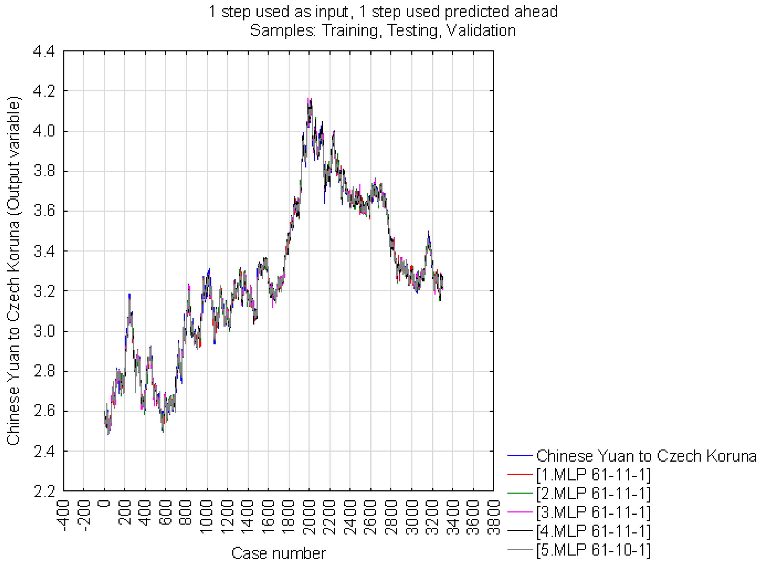
What follows next is the analogical work with the datasets. The time series was divided into three datasets (i.e., training, testing, and validation). The first dataset included 70% of the input data. The neural structures were created on the basis of the training set. Each of the two remaining datasets included 15% of the input data, respectively. Both of these datasets served to verify the reliability of the discovered neural structure (i.e., the discovered model). The time series delay was 1. In total, 100,000 neural networks were created, of which the five with the best traits were retained. The hidden layer contained at least two neurons and at most 50 neurons. For the radial basis function, the hidden layer contained at least 21 neurons and at most 30 neurons. The following distribution functions were considered for a multiple perceptron network in the hidden and output layers: Atanh, exponential, linear, logistic, and sinus. The performance of the individual datasets was defined in the form of a correlation coefficient. There were, of course, other performance measures such as root mean square error (RMSE), the mean absolute percentage error (MAPE), mean absolute bias error (MABE), and coefficient of determination (R2). The root mean square error (RMSE) is the square root of the mean square error (MSE). RMSE measures the differences between the values predicted by the hypothetical model and the observed values. In other words, it measures the quality of the fit between the actual data and the predicted model. Similarly, MAPE is a simple average of absolute percentage errors, a formula used to calculate an error in a statistical forecast that measures the magnitude of a predicted error. The coefficient of determination, R2, is a useful measure of the total value of the predictor variable(s) when predicting the resulting variable in a linear regression setting (Salkind 2010).

The other settings remained in the default (as for ANS—automated neural networks). Finally, the results of both retained sets of neural networks were compared.

4. Results

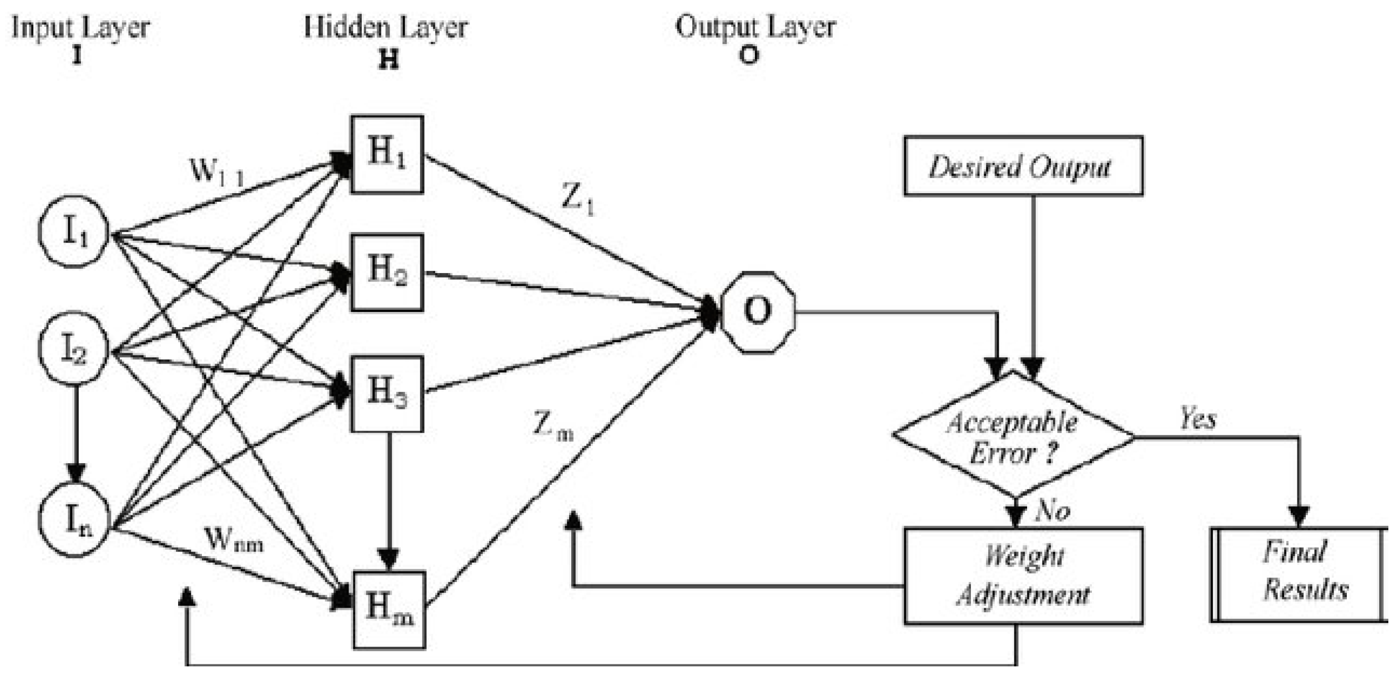
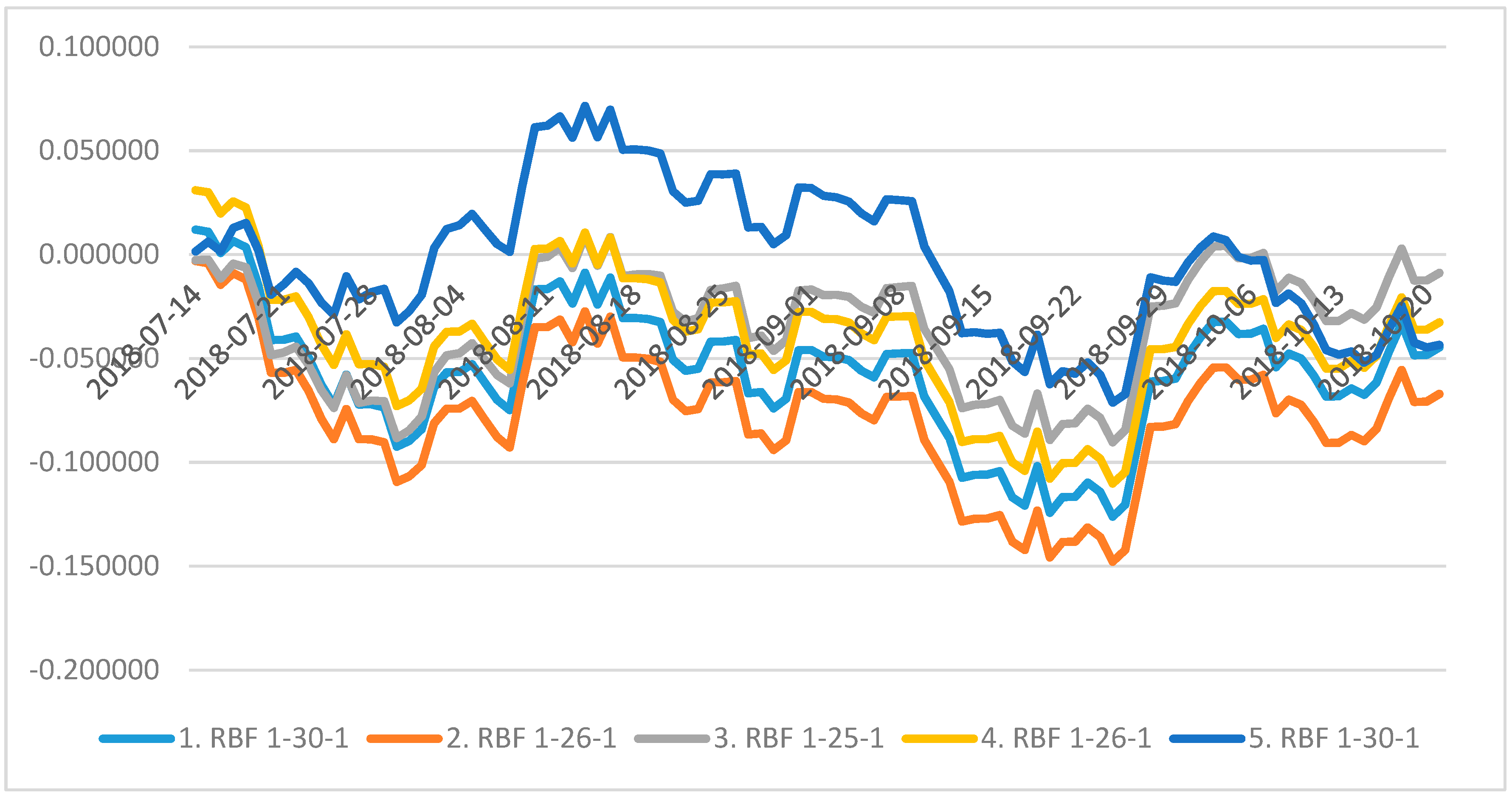
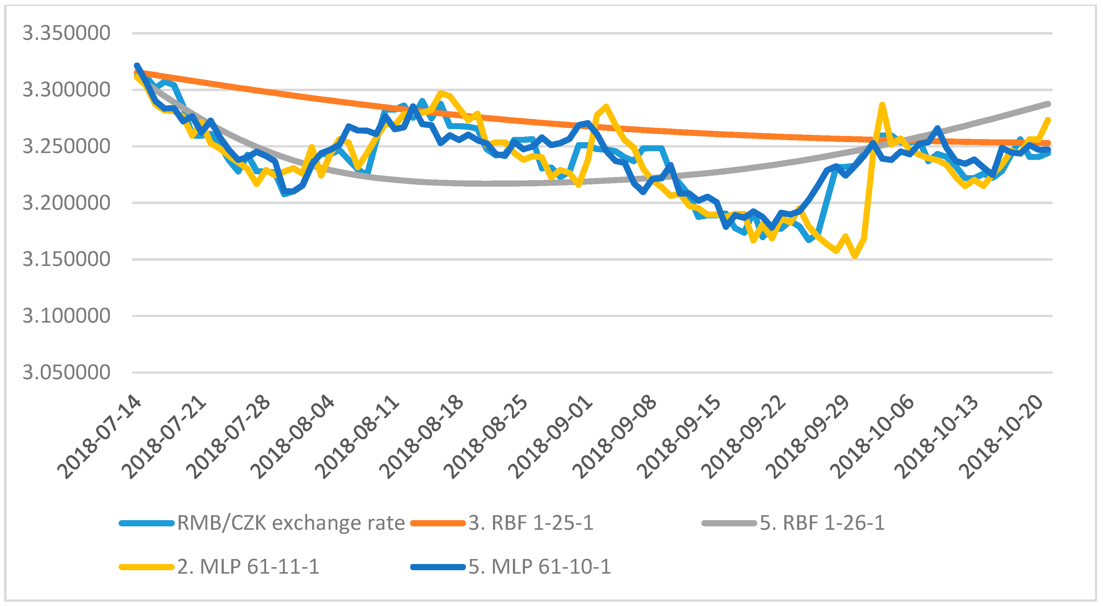
4.1. Neural Structure A

A total of 100,000 NNs were generated in the course of the above-defined procedure. The five that displayed the best parameters were retained and are presented in

Table 2. Retained neural networks.

	Network	Training Perform.	Testing Perform.	Validation Perform.	Training Error	Testing Error	Validation Error	Training Algorithm	Error Function	Activ. of Hidden Layer	Output Activ. Function
1	RBF 1-30-1	0.983490	0.983020	0.984843	0.002516	0.002616	0.002319	RBFT	Sum.quar.	Gauss	Identity
2	RBF 1-26-1	0.984841	0.985412	0.984883	0.002312	0.002255	0.002309	RBFT	Sum.quar.	Gauss	Identity
3	RBF 1-25-1	0.986071	0.986443	0.985769	0.002126	0.002109	0.002179	RBFT	Sum.quar.	Gauss	Identity
4	RBF 1-26-1	0.985491	0.985337	0.984503	0.002213	0.002262	0.002367	RBFT	Sum.quar.	Gauss	Identity
5	RBF 1-30-1	0.984297	0.983784	0.984732	0.002394	0.002499	0.002339	RBFT	Sum.quar.	Gauss	Identity

Source: Own research; according to Machova and Marecek (2019).

.

All were radial basis function NNs with only one variable in the input layer (i.e., time). The NNs contained from 25 to 30 neurons in the hidden layer. There was a solo neuron and a solo output variable (i.e., the CZK/RMB exchange rate) in the output layer. The RBFT (redundant byzantine fault tolerance) training algorithm was applied to all the networks. The hidden layer of neurons of all the neural networks was activated by the same function (i.e., the Gaussian curve). Likewise, the external layers of neurons used the same function for the purpose of activation (see Table 2). The search was for a network that performed equally well across all the datasets (note: the data distribution across the datasets took place randomly), while the error should be the smallest possible. The performance of the individual datasets was represented by a correlation coefficient. The values for the individual datasets for the retained NNs are presented in Table 2.

The figures revealed that the performance of all the retained neural networks reached approximately the same results. The unimportant differences had no impact on the performance of the respective networks. The values of the correlation coefficients for all the training datasets was below 0.983. The values of the correlation coefficients for the testing datasets were very similar to the training datasets (i.e., always above 0.983) and was above 0.984 for the validation datasets. Note that the error for all the datasets was slightly above 0.002. The error differences for the equalized time series were almost insignificant for the datasets. A more detailed analysis is required to determine the most appropriate neural network.

Table 3. Statistical characteristics of the individual datasets according to the retained neural network.

Statistics	1.RBF 1-30-1	2.RBF 1-26-1	3.RBF 1-25-1	4.RBF 1-26-1	5.RBF 1-30-1
Minimal prediction (training)	2.58183	2.55340	2.52919	2.52734	2.62556
Maximal prediction (training)	4.04950	4.09743	4.00225	4.00540	3.95151
Minimal prediction (testing)	2.58355	2.55342	2.52917	2.52741	2.62557
Maximal prediction (testing)	4.04944	4.09741	4.00223	4.00544	3.95152
Minimal prediction (validation)	2.58184	2.55531	2.53062	2.52749	2.62600
Maximal prediction (validation)	4.04951	4.09682	4.00226	4.00505	3.95129
Minimal residuals (training)	−0.22414	−0.21614	−0.30694	−0.24314	−0.28141
Maximal residuals (training)	0.37317	0.23107	0.22900	0.21521	0.29266
Minimal residuals (testing)	−0.21388	−0.18746	−0.28546	−0.22842	−0.26051
Maximal residuals (testing)	0.37307	0.23378	0.22341	0.20519	0.29323
Minimal residuals (validation)	−0.21094	−0.17494	−0.17479	−0.20650	−0.23232
Maximal residuals (validation)	0.26023	0.22773	0.18504	0.21784	0.21065
Minimal standard residuals (training)	−4.46833	−4.49505	−6.65757	−5.16815	−5.75120
Maximal standard residuals (training)	7.43936	4.80567	4.96689	4.57450	5.98108
Minimal standard residuals (testing)	−4.18178	−3.94719	−6.21611	−4.80292	−5.21090
Maximal standard residuals (testing)	7.29438	4.92251	4.86501	4.31438	5.86540
Minimal standard residuals (validation)	−4.38041	−3.64037	−3.74445	−4.24472	−4.80316
Maximal standard residuals (validation)	5.40392	4.73891	3.96396	4.47779	4.35511

Source: Machova and Marecek (2019).

provides an overview of the basic statistical characteristics of the individual datasets for the five retained neural networks.

Under ideal circumstances, the statistical characteristics of the neural networks should comply, in an interspace manner, in all the sets of a certain neural structure (i.e., minima, maxima, residuals, etc.). In the case of the retained neural networks, the differences between the equalized time series were minimal, both in terms of absolute values and residuals. It is therefore not clear which of the retained NNs generated the most suitable results. Therefore, all the neural networks seem to be applicable in practice.

Figure 3 is a line graph that shows the actual development of the CZK/RMB exchange rate at the individual intervals in a slightly different manner. The x-axis (case number) shows information about the input data (i.e., about the time series (marked by numbers due to the software settings)), whilst the y-axis shows the value of the CZK/RMB exchange rate. The blue line indicates the actual development of the exchange rate, and the other colors show the predictions according to the individually generated and retained networks (as presented in Table 2). The close similarity of the predictions of the individual networks is not important, but rather the extent of compliance to the actual development of the exchange rate. Within this context, it can be concluded that all the undistributed neural networks are seemingly very interesting. On the face of it, the basic directions of the lines, which assess the course of the CZK/RMB exchange rate, display the extremes in the development of the actual exchange rate.

Given that the network structure (as depicted in Figure 1) contains 3303 items of data on the CZK/RMB exchange rate, this may seem unclear. It is therefore appropriate to present the situation for a selected data interval. Therefore, the line graph in Figure 4 compares the actual development of the CZK/RMB exchange rate for the final 100 days of the monitored period (i.e., from 14 July to 21 October 2018.)

The graph shows that none of the retained neural networks were completely and accurately able to trace the actual course of the CZK/RMB exchange rate during the monitored period. However, it was clear that the 3.RBF 1-25-1 and 5.RBF 1-30-1 networks came the closest to reality. Their predicted values were almost identical to the actual exchange rate at the beginning of the monitored period, with more significant differences showing at the end of the monitored period. The difference in both cases was about CZK 0.08 to one RMB. Even the least accurate network, namely 2.RBF 1-26-1, differed from the actual figures for the exchange rate by less than CZK 0.011. An examination of the residuals therefore seems appropriate. The development of the residuals during the period from 14 July to 21 October 2018 is presented in Figure 5.

The graph shows that, with exception of the 5.RBF 1-30-1 network, the aggregate of the residuals for all the neural networks during the monitored period was almost zero. The residuals achieved quite high positive values in this period. To illustrate this,

Table 4. Aggregate of the residuals for the individual equalized time series.

Characteristics	1.RBF 1-24-1	2.RBF 1-29-1	3.RBF 1-30-1	4.RBF 1-28-1	5.RBF 1-26-1
Aggregate of residuals	0.150758	−1.025922566	−3.350398611	−1.785245346	−3.244516106

Source: Own research; according to Machova and Marecek (2019).

shows the aggregate of the residuals for the equalized time series.

Under ideal circumstances, if we ignore the residual fluctuations for the individual cases during the monitored period, the absolute value of the aggregates of the residuals will total zero. The absolute value of the aggregate of the residuals of the second neural network (2.RBF 1-29-1), which was nearly −1.026, was the closest to zero. In contrast, the 3.RBF 1-30-1 and 5.RBF 1-26-1 networks produced the highest aggregate of residuals in absolute terms, with values above 3. However, it is necessary to point out that this value is minimal in relation to the 3303 measurements. It is therefore possible to state that the most accomplished neural networks were 3.RBF 1-25-1 and 5.RBF 1-30-1.

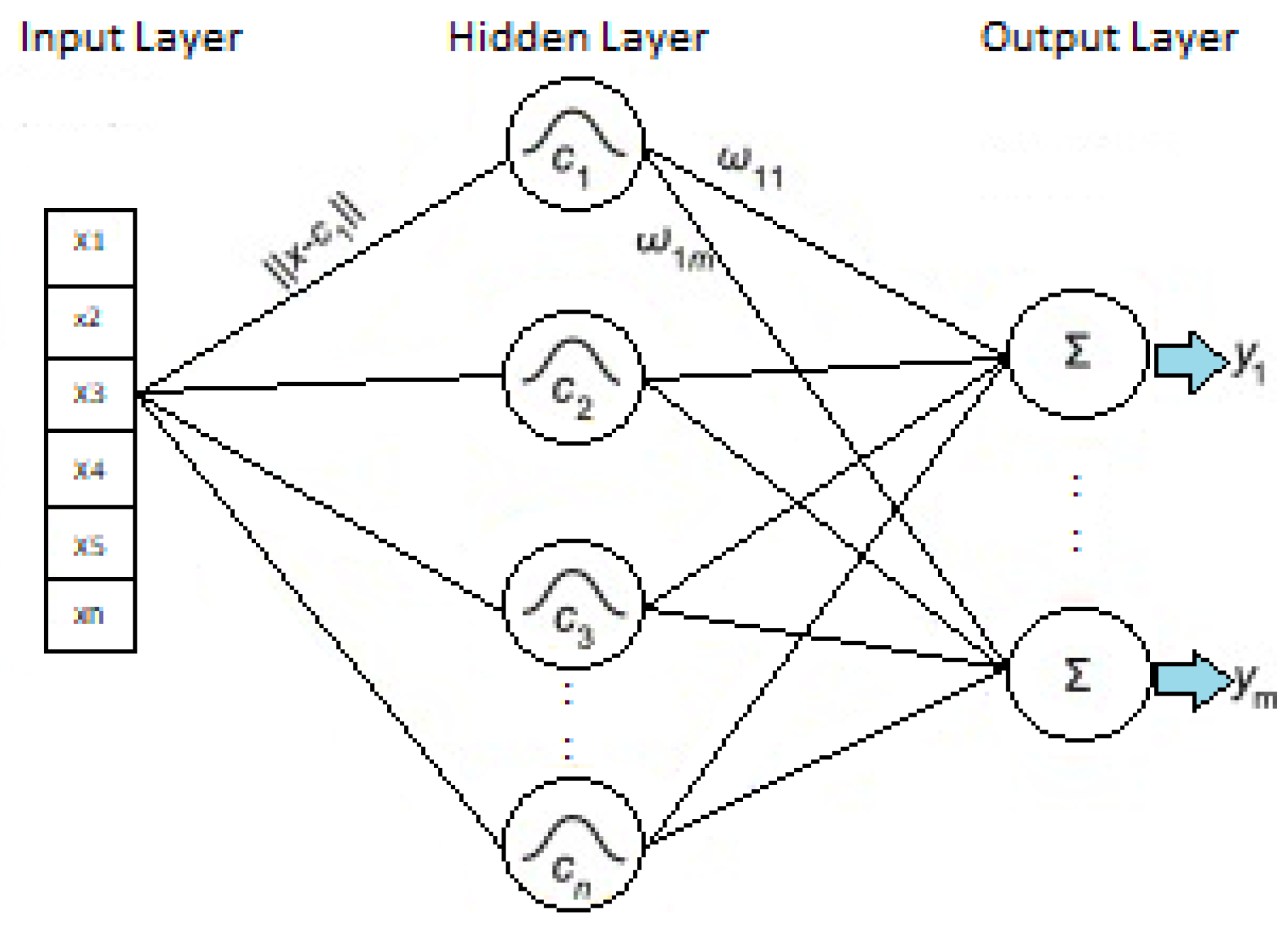
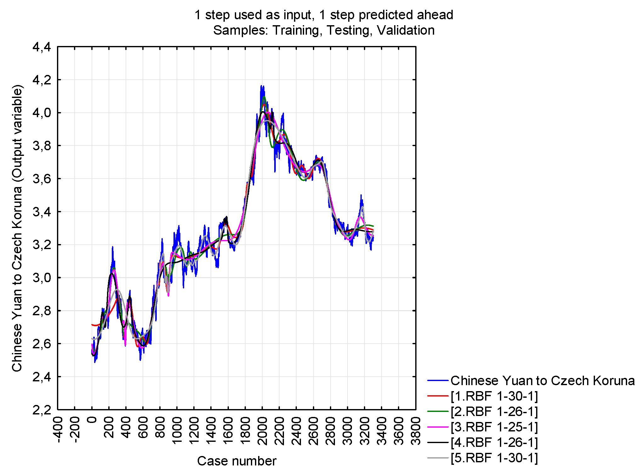
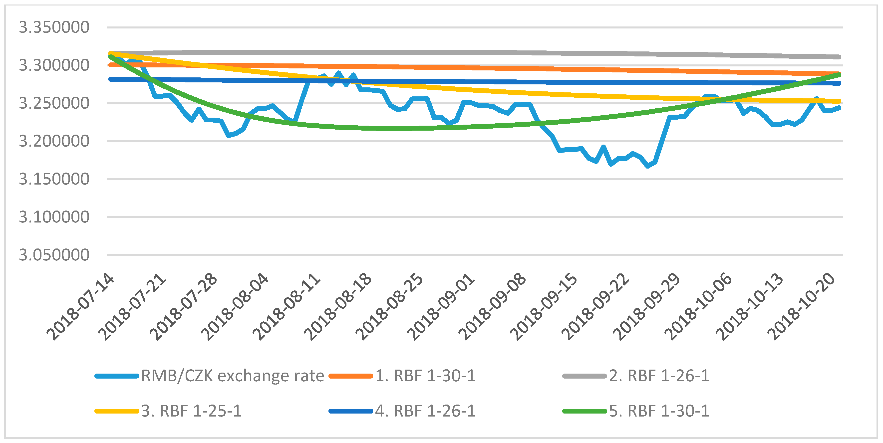
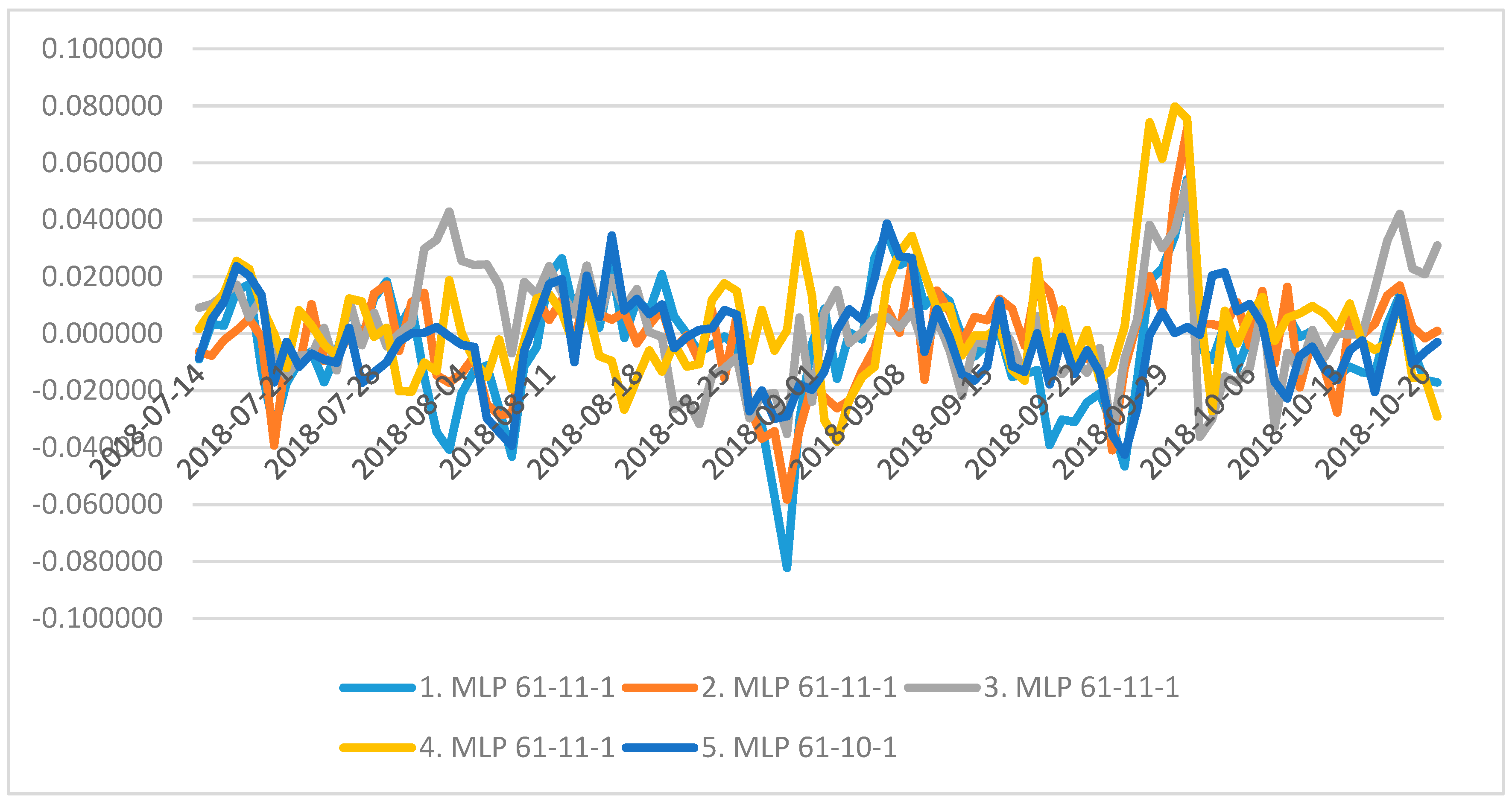
4.2. Neural Structure B

A total of 100,000 NNs were generated on the basis of the defined procedure. The five that displayed the best parameters were retained and are presented in

Table 5. Retained neural networks.

	Network	Training Perform.	Testing Perform.	Validation Perform.	Training Error	Testing Error	Validation Error	Training Algorithm	Error Function	Activ. of Hidden Layer	Output Activ. Function
1	MLP 61-11-1	0.998718	0.996990	0.997563	0.000197	0.000468	0.000374	BFGS (Quasi-Newton) 392	Sum quart.	Tanh	Identity
2	MLP 61-11-1	0.998927	0.997313	0.997517	0.000165	0.000417	0.000382	BFGS (Quasi-Newton) 461	Sum quart.	Logistic	Identity
3	MLP 61-11-1	0.998919	0.997606	0.997632	0.000166	0.000377	0.000364	BFGS (Quasi-Newton) 569	Sum quart.	Tanh	Identity
4	MLP 61-11-1	0.998791	0.997572	0.997594	0.000186	0.000377	0.000372	BFGS (Quasi-Newton) 558	Sum quart.	Tanh	Exponential
5	MLP 61-10-1	0.998640	0.997059	0.997641	0.000209	0.000457	0.000363	BFGS (Quasi-Newton) 436	Sum quart.	Tanh	Tanh

Source: Own research.

.

All were multi-layer perceptron neural networks. There were four variables (i.e., time, year, day of month, day of week, in the input layer). Time was represented by one neuron in the input layer, a year by 10 neurons, a month by 12 neurons, a weekday by 7 neurons, and a day of the month by 31 neurons, respectively. The total (i.e., 61 neurons) formed the input layer of the generated and retained neural networks. The neural networks contained either 10 or 11 neurons in the hidden layer. Consequently, there was a single neuron and a single output variable, which was the CZK/RMB exchange rate, in the output layer. The Quasi-Newton training algorithm was applied to all the networks. All the neural networks used either the hyperbolic tangent or logistic functions for the purpose of the activation of the neural hidden layer. For the activation of the neural output layer, the retained neural networks used the hyperbolic tangent, exponential, and identity functions (see Table 5).

The search was for a network that performed equally well across all the datasets (note: the data distribution across the datasets took place randomly), while the error should be the smallest possible.

The performance of the individual sets was represented by a correlation coefficient. The values for the individual datasets for the retained NNs are presented in Table 5.

The table shows that the performance of all the retained neural networks was approximately the same. The insignificant differences bear no influence on the performance of the individual networks. The values of the correlation coefficients for all the training datasets significantly exceeded 0.998. The values of the correlation coefficients for the testing datasets exceeded 0.997, and for the validation datasets, they significantly exceeded 0.997. Note that the error for all the datasets fell within the interval >0.0001 to <0.0005. The error differences for the equalized time series were completely insignificant for the individual datasets.

A more detailed analysis is required to determine the most appropriate neural network.

Table 6. Statistical characteristics of individual datasets according to the retained neural network.

Statistics	1.MLP 61-11-1	2.MLP 61-11-1	3.MLP 61-11-1	4.MLP 61-11-1	5.MLP 61-10-1
Minimal prediction (training)	5.99845	6.00641	5.99154	5.99371	6.00098
Maximal prediction (training)	9.84882	9.89527	9.87232	9.83699	9.88105
Minimal prediction (testing)	6.45895	6.46012	6.45663	6.45980	6.46002
Maximal prediction (testing)	9.95255	9.99209	9.96231	9.95287	9.99096
Minimal prediction (validation)	6.38529	6.39955	6.38028	6.38217	6.39652
Maximal prediction (validation)	9.83693	9.84308	9.83457	9.83696	9.84264
Minimal residuals (training)	−0.17159	−0.19452	−0.16813	−0.17882	−0.19039
Maximal residuals (training)	0.40824	0.50655	0.50247	0.55336	0.55220
Minimal residuals (testing)	−0.26528	−0.23472	−0.19660	−0.24778	−0.19037
Maximal residuals (testing)	0.20029	0.23874	0.22354	0.19344	0.21280
Minimal residuals (validation)	−0.18526	−0.18002	−0.17583	−0.17599	−0.17991
Maximal residuals (validation)	0.49820	0.48575	0.49862	0.49338	0.48770
Minimal standard residuals (training)	−5.65878	−5.87540	−5.56482	−5.12649	−5.87337
Maximal standard residuals (training)	14.23498	15.85302	15.20208	14.18194	15.03849
Minimal standard residuals (testing)	−5.02283	−5.74512	−6.00274	−6.12485	−5.34937
Maximal standard residuals (testing)	5.20498	4.99831	5.48930	5.40087	4.35498
Minimal standard residuals (validation)	−4.94651	−3.99879	−4.84632	−4.57713	−3.96781
Maximal standard residuals (validation)	11.59751	11.00974	11.75020	11.34307	11.01994

Source: Own research.

provides an overview of the basic statistical characteristics of the individual datasets for the five retained neural networks.

In the case of the retained neural structures, the differences over the equalized time series were minimal, both in terms of absolute values and residuals. It is therefore not clear which of the retained NNs generated the most suitable results. All the neural networks therefore seem to be applicable in practice.

Figure 6 is a line graph, which shows the actual development of the CZK/RMB exchange rate and the development of predictions with the help of the individually generated and retained networks (i.e., the equalized time series). The graph clearly shows that all the neural structures predicted the development of the CZK/RMB exchange rate almost identically. Furthermore, the course of the equalized time series was very similar to the actual course of the CZK/RMB exchange rate.

Taking into consideration that the graph illustrated in Figure 6 contains 3303 items of data on the CZK/RMB exchange rate, it may seem confusing. For this reason, it is suitable to present the situation for a selected data interval. The line graph in Figure 7 therefore compares the actual development of the CZK/RMB exchange rate for the final 100 days of the monitored period (i.e., from 14 July to 21 October 2018).

The graph clearly shows that all the neural structures were able to copy the CZK/RMB exchange rate quite well. The maximum difference across the interval was CZK 0.05. The biggest difference could be found within the period from 9/26/2018 to 10/1/2018, when the difference was still less than CZK 0.1. It is therefore possible to state on the mere basis of the graphic comparison that all the retained neural structures are usable for predictive purposes. An examination of the residuals therefore seems appropriate and interesting. The development of the residuals during the period from 14 July to 21 October is presented in Figure 8.

The graph clearly shows that the aggregate of the residuals for all neural networks during the monitored period verged on zero. To illustrate this,

Table 7. Aggregate of the residuals for the individual equalized time series.

Characteristics	1.MLP 61-11-1	2.MLP 61-11-1	3.MLP 61-11-1	4.MLP 61-11-1	5.MLP 61-10-1
Aggregate of residuals	0.632230639	0.120515671	−0.437742553	0.738084025	0.803606299

Source: Own research.

shows the aggregate of the residuals for the equalized time series.

The aggregate of the residuals for the fifth neural structure, namely 2.MLP 61-11-1, was closest to the value zero (i.e., 0.12). In contrast, the neural network with the highest value for the aggregate of the residuals (0.738) was 4.MLP 61-11-1 where the differences were absolutely minimal. It is therefore possible to conclude that all the retained neural structures are able to equalize the time series for the CZK/RMB exchange rate in a very reliable manner and are usable for the prediction of the development of the exchange rate.

5. Discussion

All the generated and retained ANNs were able to balance the examined time series (i.e., the CZK/RMB exchange rate). A comparison of the correlation coefficients clearly showed (see Table 2 and Table 5) that alternative B (i.e., the retained MLP neural networks, which include the use of additional categorical variables) was more efficient. This is reflected in Table 3 and Table 6 with regard to the evaluation of the basic statistical characteristics for predictions or equalized time series. The retained MLP neural networks (i.e., their equalized time series) generated smaller mutual differences in the training, testing, and validation datasets than the retained RBF neural networks (i.e., without an additional variable). This was confirmed in Figure 3, Figure 4, Figure 5, Figure 6, Figure 7 and Figure 8. It is very clear that only the retained MLP neural networks under neural structure B were able to describe the time series according to their actual course (for more details see Figure 9).

A number of other authors have also dealt with the prediction of exchange rates using ANN. Although their findings are interesting, they deal with a partially different application than the one addressed in this contribution.

For example, the goal of Ismail et al. (2018) was to predict the exchange rate of the US dollar expressed in Malaysian ringgit. The exchange rate prediction was performed using two methods, namely artificial neural networks and the autoregressive integrated moving average (ARIMA). To predict the exchange rate, a feed-forward neural network was chosen as the artificial neural structure because this proved to be inherently stable. On the other hand, ARIMA (0,1,1) was chosen as the best model for time series based on the Box–Jenkins method. When comparing the two methods, the authors concluded that, compared to ARIMA, the feed-forward neural network showed better results because it had a smaller mean square error and a root mean square error. The research therefore shows that for predicting the US dollar exchange rate expressed in Malaysian ringgit, the use of a feed-forward neural structure seems to be a more suitable prediction method than the ARIMA time series model (0,1,1). The neural structures highlighted in this contribution also generated very good results. The neural networks faithfully copied the development of the time series and predicted the development of the exchange rate.

Through their research, Jiang and Song (2010) demonstrated the chaotic nature of time series for exchange rates. The authors also calculated the embedding dimension and time series delay, and determined the exchange rate prediction model using the NARX network (non-linear autoregressive model). The authors used the time series for exchange rates to empirically evaluate the proposed approach for mid-period forecasting tasks. The results showed that the proposed approach consistently outperformed standard predictors based on neural networks such as BP (back propagation) or SVM (support vector machine).

It is also worth mentioning Abdullah (2013), who, on the basis of the aforementioned, predicted the MYR/USD (MYR = Malaysian Ringgit) exchange rate. In his study, the author also tested the exchange rate performance using a distance-based fuzzy time series model. MYR/USD exchange rate data were tested according to a prediction model from 11 August 2009 to 15 September 2009. A performance comparison sample was performed between MYR/USD and TWD/USD (TWD = Taiwan New Dollar) datasets. The research results showed that the predictions for MYR/USD were smaller than TWD/USD.

The application of the research presented in this contribution is also interesting. It is clear that the RMB is perceived, mainly due to the strict monetary control of the People’s Bank of China (Cheong et al. 2017), as a relatively controversial currency. On the other hand, in the current situation of relatively massive budget deficits and quantitative easing, where Aizenman et al. (2020) already point out the correlation, it is clear that for users of less important currencies (CZK, PLN, HUF, and others), it provides monetary security. Security is therefore not only to be considered through currency pairs with the USD or the EUR, respectively, but also within the framework of risk diversification and partly against the RMB. On one hand, this approach presents risks due to the potential for trade wars between China and the United States (Liu and Woo 2018), but it also presents extraordinary opportunities. As Ding et al. (2020), who analyzed the link between RMB and the price of oil, and Kunze (2019) stated, the controlled exchange rate can act as a stabilizing element, or even as a refining factor for predictions. However, high-quality analytical-predictive tools are absolutely necessary for this approach. This is exactly what has been provided by this study.

6. Conclusions

The aim of this contribution was to put forward a methodology for how to account for seasonal variations in the process of equalizing time series for the CZK/RMB exchange rate through the use of ANNs. In general, the fulfilment of every forecast is, to a certain degree, determined by the probability this will occur on its own. When predicting the future development of any variable, there is an attempt to estimate the evolution of this variable on the basis of past data. Even though we are able to integrate the majority of factors that influence the target quantity into a model, there is always an element of simplification involved. It is for this reason that a certain degree of probability that a predicted scenario will take place is always taken into account. This can be considered as a limitation of the research, as can the use of basic types of NNs and the comparison of this method with the results of other suitable alternatives.

This contribution refers to the application of an identical instrument to various initial tasks. Prior to the experiment, the assumption was made that there was no reason to apply categorical variables in order to describe the seasonal fluctuations in the CZK/RMB exchange rate. However, the opposite turned out to be true. Extra variables-in the form of a year, a month, day of month, and day of week–the values of which were determined—brought better order and accuracy into the time series. The development of the CZK/RMB exchange rate can be defined on the basis of any statistical, causal, or easy-to-use methods. In this case, statistical methods were used. However, these only provided us with a potential framework for future development. Within this context, it is also important to consider possible future developments in economic policy and/or the legal environment. At the same time, the personality of the evaluator is of equal importance. Generally speaking, they are economists who correct the price defined by the framework methods and modify them on the basis of casual relations and/or on the basis of their experience and knowledge. Nevertheless, in this case, it seems appropriate to try to make a prediction using neural structure B, which is quite accurate.

The results of the MPL networks were very interesting. The objective of this contribution was therefore fulfilled. Interestingly, in the case of neural structure A, only radial basis function neural networks were retained as the most successful, whereas multi-layer perceptron neural networks were the most successful for neural structure B. What would have been interesting would have been to generate only one type of neural network for a specific situation (i.e., every time in a different manner from the acquired results (for alternative A, an MPL network, and for alternative B, an RBF network)).

In further research, it would also be interesting to compare the performance of neural structures with the performance of other models used for time series predictions such as ARIMA models, assuming the use of identical data. However, this would still require the use of statistical methods, which, once again, only provide a possible framework for exchange rate developments. As a result, it would be desirable to include information on the development of the economic, political, and/or legal environments in the model. Where it is possible to do so and to predict such developments, it will then be possible to project this into the monitored variable accordingly.

References

1. Abdullah, Lazim. 2013. Performance of exchange rate forecast using distance-based fuzzy time series. International Journal of Engineering and Technology 5: 452–59. [Google Scholar]
2. Accominotti, Olivier, Jason Cen, David Chambers, and Ian W. Marsh. 2019. Currency regimes and the carry trade. Journal of Financial and Quantitative Analysis 54: 2233–60. [Google Scholar] [CrossRef] [Green Version]
3. Aizenman, Joshua, Yin-Wong Cheung, and Xiangwang Qian. 2020. The currency composition of international reserves, demand for international reserves, and global safe assets. Journal of International Money and Finance 102. [Google Scholar] [CrossRef]
4. Alonso-Monsalve, Saúl, Andrés L. Suarez-Cetrulo, Alejandro Cervantes, and David Quintana. 2020. Convolution on neural networks for high-frequency trend prediction of cryptocurrency exchange rates using technical indicators. Expert Systems with Applications 149. [Google Scholar] [CrossRef]
5. Amo Baffour, Alexander, Jingchun Feng, and Evans Kwesi Taylor. 2019. A hybrid artificial neural network-GJR modeling approach to forecasting currency exchange rate volatility. Neurocomputing 365: 285–301. [Google Scholar] [CrossRef]
6. Arneric, Josip, Tea Poklepovic, and Zdravka Aljinovic. 2014. GARCH based artificial neural networks in forecasting conditional variance of stock returns. Croatian Operational Research Review 5: 329–43. [Google Scholar] [CrossRef] [Green Version]
7. Augustin, Patrick, Mikhail Chernov, and Dongho Song. 2020. Sovereign credit risk and exchange rates: Evidence from CDS quanto spreads. Journal of Financial Economics 137: 129–51. [Google Scholar] [CrossRef]
8. Bahmani-Oskooee, Mohsen, and Scott W. Hegerty. 2007. Exchange rate volatility and trade flows: A review article. Journal of Economic Studies 34: 211–55. [Google Scholar] [CrossRef]
9. Bernard, Andrew B. 2004. Exporting and productivity in the USA. Oxford Review of Economic Policy 20: 343–57. [Google Scholar] [CrossRef]
10. Bielecki, Anrzej, Pawel Hajto, and Robert Schaefer. 2008. Hybrid neural systems in exchange rate prediction. Studies in Computational Intelligence: Natural Computing in Computational Finance 100: 211–30. [Google Scholar] [CrossRef]
11. Bodart, Vincent, and Jean-Francois Carpantier. 2020. Currency collapses and output dynamics in commodity dependent countries. Emerging Markets Review 42. [Google Scholar] [CrossRef]
12. Bonadio, Barthélémy, Andreas Fischer, and Philip Sauré. 2020. The speed of exchange rate pass-through. Journal of the European Economic Association 18: 506–38. [Google Scholar] [CrossRef]
13. Budikova, Marie, Maria Kralova, and Bohumil Maros. 2010. Průvodce Základními Statistickými Metodami [Guide to Basic Statistical Methods]. Prague: Grada. [Google Scholar]
14. Bulut, Levent. 2018. Google Trends and the forecasting performance of exchange rate models. Journal of Forecasting 37: 303–15. [Google Scholar] [CrossRef]
15. Cai, Zongwu, Linna Chen, and Ying Fang. 2012. A new forecasting model for USD/CNY exchange rate. Studies on Nonlinear Dynamics and Econometrics 16. [Google Scholar] [CrossRef] [Green Version]
16. Chari, V.V., Alessandro Dovis, and Patrick J. Kehoe. 2020. Rethinking optimal currency areas. Journal of Monetary Economics 111: 80–94. [Google Scholar] [CrossRef] [Green Version]
17. Cheong, Calvin W.H., Jothee Sinnakkannu, and Sockalingam Ramasamy. 2017. On the predictability of carry trade returns: The case of the Chinese Yuan. Research in International Business and Finance 39: 358–76. [Google Scholar] [CrossRef]
18. Cheong, Chongcheul, Tesfa Mehari, and Leighton Vaughan Williams. 2006. Dynamic links between unexpected exchange rate variation, prices, and international trade. Open Economies Review 17: 221–33. [Google Scholar] [CrossRef]
19. Chernov, Mikhail, Jeremy Graveline, and Irina Zviadadze. 2018. Crash risk in currency returns. Journal of Financial and Quantitative Analysis 53: 137–70. [Google Scholar] [CrossRef] [Green Version]
20. Cheung, Yin-Wong, Cho-Hoi Hui, and Andrew Tsang. 2018. Renminbi central parity: An empirical investigation. Pacific Economic Review 23: 164–83. [Google Scholar] [CrossRef] [Green Version]
21. Cheung, Yin-Wong, Menzie D. Chinn, Antonio Garcia Pascual, and Yi Zhang. 2019. Exchange rate prediction redux: New models, new data, new currencies. Journal of International Money and Finance 95: 332–62. [Google Scholar] [CrossRef] [Green Version]
22. Chiappini, Raphael, and Delphine Lahet. 2020. Exchange rate movements in emerging economies—Global vs regional factors in Asia. China Economic Review 60. [Google Scholar] [CrossRef]
23. Cho, Jae-Beom, Hong-Ghi Min, and Judith Ann McDonald. 2020. Volatility and dynamic currency hedging. Journal of International Financial Markets, Institutions and Money 64. [Google Scholar] [CrossRef]
24. Choi, Yoonho, and E. Kwan Choi. 2018. Unemployment and optimal exchange rate in an open economy. Economic Modelling 69: 82–90. [Google Scholar] [CrossRef]
25. Colacito, Ric, Mariano M. Croce, Federico Gavazzoni, and Robert Ready. 2018. Currency risk factors in a recursive multicountry economy. The Journal of Finance 73: 2719–56. [Google Scholar] [CrossRef]
26. Dahlquist, Magnus, and Henrik Hasseltoft. 2020. Economic momentum and currency returns. Journal of Financial Economics 136: 152–67. [Google Scholar] [CrossRef] [Green Version]
27. De Baets, Shari, and Nigel Harvey. 2018. Forecasting from time series subject to sporadic perturbations: Effectiveness of different types of forecasting support. International Journal of Forecasting 34: 163–80. [Google Scholar] [CrossRef]
28. De Boer, Jantke, Kim J. Bövers, and Steffen Meyer. 2020. Business cycle variations in exchange rate correlations: Revisiting global currency hedging. Finance Research Letters 33. [Google Scholar] [CrossRef]
29. Dhamija, Ajay K., and V. K. Bhalla. 2011. Exchange rate forecasting: comparison of various architectures of neural networks. Neural Computing and Applications 20: 355–63. [Google Scholar] [CrossRef]
30. Ding, Haoyuan, Yuying Jin, Cong Qin, and Jiezhou Ying. 2020. Tail causality between crude oil price and RMB exchange rate. China & World Economy 28: 116–34. [Google Scholar] [CrossRef]
31. Dogru, Tarik, Cem Isik, and Ercan Sirakaya-Turk. 2019. The balance of trade and exchange rates: Theory and contemporary evidence from tourism. Tourism Management 74: 12–23. [Google Scholar] [CrossRef]
32. Dunis, Christian L., Jason Laws, and Georgios Sermpinis. 2011. Higher order and recurrent neural architectures for trading the EUR/USD exchange rate. Quantitative Finance 11: 615–29. [Google Scholar] [CrossRef]
33. Faris, Hossam, Ibrahim Aljarah, and Seyedali Mirjalili. 2017. Evolving Radial Basis Function networks using Moth-Flame optimizer. Handbook of Neural Computation, 537–50. [Google Scholar] [CrossRef]
34. Forbes, Kristin, Ida Hjortsoe, and Tsvetelina Nenova. 2018. The shocks matter: Improving our estimates of exchange rate pass-through. Journal of International Economics 114: 255–75. [Google Scholar] [CrossRef] [Green Version]
35. Foreign Direct Investment. 2018–2019. Obecný metodický popis a komentář k vývoji přímých zahraničních investic [General methodological description and commentary on the development of foreign direct investment]. In Www.cnb.cz. Prague: Czech National Bank. [Google Scholar]
36. Gopinath, Gita, Emine Boz, Camila Casas, Federico J. Díez, Pierre-Olivier Gourinchas, and Mikkel Plagborg-Møller. 2020. Dominant currency paradigm. American Economic Review 110: 677–719. [Google Scholar] [CrossRef] [Green Version]
37. Grabowski, Wojciech, and Aleksander Welfe. 2020. The Tobit cointegrated vector autoregressive model: An application to the currency market. Economic Modelling 89: 88–100. [Google Scholar] [CrossRef]
38. Groll, Dominik, and Tommaso Monacelli. 2020. The inherent benefit of monetary unions. Journal of Monetary Economics 111: 63–79. [Google Scholar] [CrossRef] [Green Version]
39. Guresen, Erkam, Gulgun Kayakutlu, and Tugrul U. Daim. 2011. Using artificial neural network models in stock market index prediction. Expert systems with Applications 38: 10389–97. [Google Scholar] [CrossRef]
40. Ha, Jongrim, M. Marc Stocker, and Hakan Yilmazkuday. 2020. Inflation and exchange rate pass-through. Journal of International Money and Finance 105. [Google Scholar] [CrossRef] [Green Version]
41. Han, Liyan, Li Wan, and Yang Xu. 2020. Can the Baltic Dry Index predict foreign exchange rates? Finance Research Letters 32. [Google Scholar] [CrossRef]
42. Henriquez, Jonatan, and Werner Kristjanpoller. 2019. A combined independent component analysis-neural network model for forecasting exchange rate variation. Applied Soft Computing 83. [Google Scholar] [CrossRef]
43. Hnat, Pavel, and Martin Tlapa. 2014. China-V4 Investment regime–a Czech perspective. Paper presented at Trends and Perspectives in Development of China-V4 Trade and Investment, Bratislava, Slovakia, March 12–14; pp. 82–95. [Google Scholar]
44. Ho, Chi Ming. 2020. Does virtual currency development harm financial stocks’ value? Comparing Taiwan and China markets. Economic Research-Ekonomska Istraživanja 33: 361–78. [Google Scholar] [CrossRef]
45. Ho, S. F., and Norzitah Abdul Karim. 2012. Exchange rate, macroeconomic fundamentals and international trade. 2012 IEEE Colloquium on Humanities, Science and Engineering Research, 534–38. [Google Scholar] [CrossRef]
46. Horak, Jakub, and Veronika Machova. 2019. Comparison of neural networks and regression time series on forecasting development of US imports from the PRC. Littera Scripta 12: 22–36. [Google Scholar]
47. Horak, Jakub. 2019. Using artificial intelligence to analyse businesses in agriculture industry. Paper presented at SHS Web of Conferences–Innovative Economic Symposium 2018 Innovative Economic Symposium 2018: Milestones and Trend of World Economy, Beijing, China, November 8–9; vol. 61. [Google Scholar] [CrossRef]
48. Huang, Shupei, Haizhong An, and Brian Lucey. 2020. How do dynamic responses of exchange rates to oil price shocks co-move? From a time-varying perspective. Energy Economics 86. [Google Scholar] [CrossRef]
49. Ilzetzki, Ethan, Carmen M. Reinhart, and Kenneth S. Rogoff. 2019. Exchange arrangements entering the twenty-first century: Which anchor will hold? The Quarterly Journal of Economics 134: 599–646. [Google Scholar] [CrossRef] [Green Version]
50. Ismail, Munira, Nurul Zafirah Jubley, and Zalina Mohd Ali. 2018. Forecasting Malaysian Foreign exchange rate using artificial neural network and ARIMA time series. Paper presented at International Conference on Mathematics, Engineering and Industrial Applications, Kuala Lumpur, Malaysia, July 24–26; vol. 2013. [Google Scholar] [CrossRef]
51. Jiang, Chuanjin, and Fugen Song. 2010. Forecasting chaotic time series of exchange rate based on nonlinear autoregressive model. Paper presented at 2nd IEEE International Conference on Advanced Computer Control, ICACC, Shenyang, China, March 27–29; vol. 5, pp. 238–41. [Google Scholar] [CrossRef]
52. Khademalomoom, Siroos, and Paresh Kumar Narayan. 2020. Intraday-of-the-week effects: What do the exchange rate data tell us? Emerging Markets Review 43. [Google Scholar] [CrossRef]
53. Khalafi, Farshad Faghihi H., and Seyed Mohammad Mirvakili. 2011. A literature survey of neutronics and thermal-hydraulics codes for investigating reactor core parameters; artificial neural networks as the VVER-1000 core predictor. Nuclear Power–System Simulations and Operation, 103–22. [Google Scholar] [CrossRef] [Green Version]
54. Kharrat, Sabrine, Yacine Hammami, and Ibrahim Fatnassi. 2020. On the cross-sectional relation between exchange rates and future fundamentals. Economic Modelling 89: 484–501. [Google Scholar] [CrossRef]
55. Kriwoluzky, Alexander, Gernot J. Müller, and Martin Wolf. 2019. Exit expectations and debt crises in currency unions. Journal of International Economics 121. [Google Scholar] [CrossRef] [Green Version]
56. Kunze, F. 2019. Predicting exchange rates in Asia: New insights on the accuracy of survey forecasts. Journal of Forecasting 39: 313–33. [Google Scholar] [CrossRef] [Green Version]
57. Laily, Vania Orva Nur, Budi Warsito, and Di Asih I. Maruddani. 2018. Comparison of ARCH/GARCH model and Elman Recurrent Neural Network on data return of closing price stock. Paper presented at 7th International Seminar on New Paradigm and Innovation on Natural Science and its Application, Semarang, Indonesia, October 17. [Google Scholar]
58. León-Alvarez, Alba Luz, Jorge Iván Betancur-Gomez, Fabián Jaimes-Barragan, and Hugo Grisales-Romero. 2016. Ronda clínica y epidemiológica. Series de tiempo. IATREIA 29: 373–81. [Google Scholar] [CrossRef] [Green Version]
59. Li, Nan, Liepeng Sun, Xiao Luo, Rong Kang, and Mingde Jia. 2019. Foreign trade structure, opening degree and economic growth in Western China. Economies 7: 56. [Google Scholar] [CrossRef] [Green Version]
60. Liu, Li, Siming Tan, and Yudong Wang. 2020. Can commodity prices forecast exchange rates? Energy Economics 87. [Google Scholar] [CrossRef]
61. Liu, Tao, and Wing Thye Woo. 2018. Understanding the U.S.-China trade war. China Economic Journal 11: 319–40. [Google Scholar] [CrossRef]
62. Liu, Zhao Cheng, Xi Yu Liu, and Zi Ran Zheng. 2011. Modeling and prediction of the CNY exchange rates using RBF neural networks versus GARCH models. Quantum, Nano, Micro and Information Technologies 36: 375–82. [Google Scholar] [CrossRef]
63. Lu, Xunfa, Danfeng Que, and Guangxi Cao. 2016. Volatility forecast based on the hybrid artificial neural network and GARCH-type models. Paper presented at Promoting Business Analytics and Quantitative Management of Technology: 4th International Conference on Information Technology and Quantitative Management, Asan, Korea, August 16–18; pp. 1044–49. [Google Scholar] [CrossRef] [Green Version]
64. Ma, Guonan, and Robert N. Mccauley. 2011. The implications of Renminbi basket management for Asian currency stability. Frontiers of Economics and Globalization: Evolving Role of Asia in Global Finance 9: 97–121. [Google Scholar] [CrossRef]
65. Machova, Veronika, and Jan Marecek. 2019. Estimation of the development of Czech Koruna to Chinese Yuan exchange rate using artificial neural networks. Paper presented at SHS Web of Conferences–Innovative Economic Symposium 2018: Milestones and Trend of World Economy, Beijing, China, November 8–9; vol. 61. [Google Scholar] [CrossRef]
66. Maggiori, Matteo, Brent Neiman, and Jesse Schreger. 2020. International currencies and capital allocation. Journal of Political Economy 128: 2019–66. [Google Scholar] [CrossRef]
67. Mai, Yong, Huan Chen, Jun-Zhong Zou, and Sai-Ping Li. 2018. Currency co-movement and network correlation structure of foreign exchange market. Physica A: Statistical Mechanics and Its Applications 492: 65–74. [Google Scholar] [CrossRef]
68. Maurer, Thomas A., Thuy-Duong Tô, and Ngoc-Khanh Tran. 2019. Pricing risks across currency denominations. Management Science 65: 5308–36. [Google Scholar] [CrossRef]
69. Min, Yujuana, and Oh Suk Yang. 2019. The impact of exchange volatility exposure on firms’ foreign-denominated debts. Management Decision 57: 3035–60. [Google Scholar] [CrossRef]
70. Mohamed, Rania Ahmed Hamed. 2013. A comparison between the models ARIMA/GARCH and artificial neural networks in modelling financial returns to the Arab Republic of Egypt market securities. Advances and Applications in Statistics 36: 131–50. [Google Scholar]
71. Narayan, Paresh Kumar, Susan Sunila Sharma, Ding Hoang Bach Phan, and Guangqiang Liu. 2020. Predicting exchange rate returns. Emerging Markets Review 42. [Google Scholar] [CrossRef]
72. Nguyen, Thi-Ngoc Anh, and Kiyotaka Sato. 2020. Invoice currency choice, nonlinearities and exchange rate pass-through. Applied Economics 52: 1048–69. [Google Scholar] [CrossRef]
73. Opie, Wei, and Steven J. Riddiough. 2020. Global currency hedging with common risk factors. Journal of Financial Economics 136: 780–805. [Google Scholar] [CrossRef]
74. Ornelas, José Renato Haas, and Roberto Baltieri Mauad. 2019. Implied volatility term structure and exchange rate predictability. International Journal of Forecasting 35: 1800–13. [Google Scholar] [CrossRef]
75. Ortiz Arango, Francisco. 2017. Prognosis of oil prices: A comparison between GARCH models and differential neural networks. Investigacion Economica 73: 105–26. [Google Scholar] [CrossRef]
76. Parot, Alejandro, Kevin Michell, and Werner D. Kristjanpoller. 2019. Using artificial neural networks to forecast exchange rate, including VAR-VECM residual analysis and prediction linear combination. Intelligent Systems in Accounting Finance & Management 26: 3–15. [Google Scholar] [CrossRef] [Green Version]
77. Petrica, Andreea Cristina, and Stelian Stancu. 2017. Empirical results of modelling EUR/RON exchange rate using ARCH, GARCH, EGARCH, TARCH and PARCH models. Romanian Statistical Review, 57–72. [Google Scholar]
78. Ponomareva, Natalia, Jeffrey Sheen, and Ben Zhe Wang. 2019. Forecasting exchange rates using principal components. Journal of International Financial Markets, Institutions and Money 63. [Google Scholar] [CrossRef]
79. Quaicoe, Michael Techie, Frank B. K. Twenefour, Emmanuel M. Baah, and Ezekiel N. N. Nortey. 2015. Modeling variations in the cedi/dollar exchange rate in Ghana: An autoregressive conditional geteroscedastic (ARCH) models. Springerplus 4. [Google Scholar] [CrossRef] [Green Version]
80. Rajković, Milos, Predrag Bjelić, Danijela Jaćimović, and Miroslav Verbič. 2020. The impact of the exchange rate on the foreign trade imbalance during the economic crisis in the new EU member states and the Western Balkan countries. Economic Research-Ekonomska Istraživanja 33: 182–203. [Google Scholar] [CrossRef]
81. Ramchoun, Hassan, Mohammed Amine Janati Idrissi, Youssef Ghanou, and Mohamed Ettaouil. 2017. New modeling of multilayer perceptron architecture optimization with regularization: An application to pattern classification. IAENG International Journal of Computer Science 44: 261–69. [Google Scholar]
82. Ribeiro, Rafael S. M., John S. L. Mccombie, and Gilberto Tadeu Lima. 2020. Does real exchange rate undervaluation really promote economic growth? Structural Change and Economic Dynamics 52: 408–17. [Google Scholar] [CrossRef]
83. Salkind, Neil J. 2010. Encyclopedia of Research Design. Thousand Oaks: SAGE Publications. [Google Scholar] [CrossRef]
84. Sheikhan, Mansour, Najmeh Mohammadi, and Robert Schaefer. 2013. Time series prediction using PSO-optimized neural network and hybrid feature selection algorithm for IEEE load data. Neural Computing and Applications 23: 1185–94. [Google Scholar] [CrossRef]
85. Sindelarova, Irena. 2012. Exchange rate prediction: A wavelet-neural approach. Paper presented at 30th International Conference Mathematical Methods in Economics, Karvina, Czech Republic, September 11–13; pp. 875–78. [Google Scholar]
86. Smallwood, Aaron D. 2019. Analyzing exchange rate uncertainty and bilateral export growth in China: A multivariate GARCH-based approach. Economic Modelling 82: 332–44. [Google Scholar] [CrossRef]
87. Tian, Gary Gang, and Shiguang Ma. 2010. The relationship between stock returns and the foreign exchange rate: The ARDL approach. Journal of the Asia Pacific Economy 15: 490–508. [Google Scholar] [CrossRef]
88. Turkington, David, and Alireza Yazdani. 2020. The equity differential factor in currency markets. Financial Analysts Journal 76: 70–81. [Google Scholar] [CrossRef] [Green Version]
89. Vochozka, Marek, and Jaromir Vrbka. 2019. Estimation of the development of the Euro to Chinese Yuan exchange rate using artificial neural networks. Paper presented at SHS Web of Conferences–Innovative Economic Symposium 2018: Milestones and Trend of World Economy, Beijing, China, November 8–9; vol. 61. [Google Scholar]
90. Vochozka, Marek, Jakub Horak, and Petr Suler. 2019. Equalizing seasonal time series using artificial neural networks in predicting the Euro-Yuan exchange rate. Journal of Risk and Financial Management 12: 76. [Google Scholar] [CrossRef] [Green Version]
91. Vochozka, Marek, Zuzana Rowland, Petr Suler, and Josef Marousek. 2020. The influence of the international price of oil on the value of the EUR/USD exchange rate. Journal of Competitiveness 19: 167–90. [Google Scholar] [CrossRef]
92. Vrbka, Jaromir, Petr Suler, Veronika Machova, and Jakub Horak. 2019. Considering seasonal fluctuations in equalizing time series by means of artificial neural networks for predicting development of USA and People’s Republic of China trade balance. Littera Scripta 12: 178–93. [Google Scholar] [CrossRef]
93. Wen, Tiange, and Gang-Jin Wang. 2020. Volatility connectedness in global foreign exchange markets. Journal of Multinational Financial Management 54. [Google Scholar] [CrossRef]
94. World Bank. 2020. Official Exchange Rate. Available online: https://data.worldbank.org/indicator/PA.NUS.FCRF (accessed on 20 April 2020).
95. Xing, Yuqing. 2018. Rising wages, yuan’s appreciation and China’s processing exports. China Economic Review 48: 114–22. [Google Scholar] [CrossRef]
96. Yin, Dian, and Wanyi Chen. 2016. The forecast of USD/CNY exchange rate based on the Elman neural network with volatility updating. Paper presented at 35th Chinese Control Conference, Chengdu, China, July 27–29; pp. 9562–66. [Google Scholar] [CrossRef]
97. You, Yu, and Xiaochun Liu. 2020. Forecasting short-run exchange rate volatility with monetary fundamentals: A GARCH-MIDAS approach. Journal of Banking & Finance 116. [Google Scholar] [CrossRef]
98. Zhang, Gioqinang, and Michael Y. Hu. 1998. Neural network forecasting of the British Pound/US Dollar exchange rate: comparison of various architectures of neural networks. Omega 26: 495–506. [Google Scholar] [CrossRef]
99. Zhang, Zhaoyong, and Kiyotaka Sato. 2012. Should Chinese Renminbi be blamed for its trade surplus? A structural VAR approach. The World Economy 35: 632–50. [Google Scholar] [CrossRef]
Figure 1. MLP network structure (Source: Khalafi and Mirvakili 2011).
Risks 09 00001 g001
Figure 2. RBF network structure (Source: Faris et al. 2017).
Risks 09 00001 g002
Figure 3. Actual and predicted (according to retained neural networks) development of CZK/RMB exchange rate during the monitored period (Source: Own research; according to Machova and Marecek 2019).
Risks 09 00001 g003
Figure 4. Actual and predicted (according to retained neural networks) development of the CZK/RMB exchange rate for the period from 14 July to 21 October 2018 (Source: Own research; according to Machova and Marecek 2019).
Risks 09 00001 g004
Figure 5. Development of residuals for the equalized time series during the period from 14 July to 21 October (Source: Own research; according to Machova and Marecek 2019).
Risks 09 00001 g005
Figure 6. Actual and predicted (according to retained neural networks) development of the CZK/RMB exchange rate during the monitored period (Source: Own research).
Risks 09 00001 g006
Figure 7. Actual and predicted (according to retained neural networks) development of the CZK/RMB exchange rate for the period from 14 July to 21 October 2018 (Source: Own research).
Risks 09 00001 g007
Figure 8. Development of residuals for the equalized time series during the period from 14 July to 21 October (Source: Own research).
Risks 09 00001 g008
Figure 9. Comparison of selected neural networks for equalized time series for thee CZK/RMB exchange rate during the period from 14 July to 21 October 2018 (Source: Own research).
Risks 09 00001 g009