Abstract
We propose an Explainable AI model that can be employed in order to explain why a customer buys or abandons a non-life insurance coverage. The method consists in applying similarity clustering to the Shapley values that were obtained from a highly accurate XGBoost predictive classification algorithm. Our proposed method can be embedded into a technologically-based insurance service (Insurtech), allowing to understand, in real time, the factors that most contribute to customers’ decisions, thereby gaining proactive insights on their needs. We prove the validity of our model with an empirical analysis that was conducted on data regarding purchases of insurance micro-policies. Two aspects are investigated: the propensity to buy an insurance policy and the risk of churn of an existing customer. The results from the analysis reveal that customers can be effectively and quickly grouped according to a similar set of characteristics, which can predict their buying or churn behaviour well.
1. Introduction
The performance of the insurance sector is undergoing a transformation. While life insurance products are performing well in term of market penetration, non-life products are lagging behind. This may be detrimental to the society, as the aim of the insurance industry is, in its essence, a protective one, which serves as an hedge against the risk of contingent or uncertain losses, thus generating efficiency.
The gap of the non-life insurance sector may be the manifestation of the inability of traditional insurance companies to successfully complete the so-called “last mile”: the effective communication to the final users of the importance of covering risks, either because they are not using the right tools or simply because they can not offer the protection the customers need. In order to close the gap, customers need to be understood, and effective communication is needed.
Technology based insurance (Insurtech), which is based on the application of Artificial Intelligence methods to data retrieved from users’ engagement via smartphones, can close the gap between non-life insurance providers and consumers, thereby improving the protection and resilience of our societies. The advantage of using AI applications are, in a nutshell, the capability for insurance companies to better understand consumer needs, listening to their preferences, as expressed by smartphone generated data; and, the possibility for insurance consumers to receive an insurance coverage that well fit their needs.
The application of Artificial Intelligence to insurance is relatively recent. Bernardino (2020) provides an up-to-date review of the application of AI to the insurance sector, and of the related opportunities. With the insurance sector being highly regulated, artificial intelligence applications, to be trustworthy, must be accurate and explainable: see, for example European Commission (2020).
In the introduction, we propose applying an accurate and explainable machine learning method, based on Shapley values (see Joseph 2019; Murdoch et al. 2019), to the non-life insurance industry, which can help to turn “black box” unexplainable algorithms into something closer to a white box. The application of Shapley values can shift the perspective and gain insights into customers’ needs and behaviour, building relevant profiles and going more towards prescriptive analytics.
We show the advantages of our proposal within a case study that aimed at estimating the probability of buying (or churning) a specific non-life insurance product. We then show the utility of the proposed model in order to highlight customers who are at risk of churn. In both cases, we are able to estimate the amount of opportunity/risk at both the individual and overall level, while analysing the factors that are responsible for it.
2. Methodology
2.1. Building a Predictive Classifier
The first step of our proposal is to select a highly accurate predictive model. The research literature shows that ensemble methods, consisting in the combination of several different learners to obtain low variation and low bias predictors are particularly suited for this kind of problems (see e.g., Breiman 2000). Ensembles that are made up of classification trees, which natively capture interactions and non linearities, are particularly suited for predictive classification problems. Among the family of ensemble trees learner, we employ Extreme Gradient Boosting. This algorithm consistently scores better against its peers, and it implements a gradient boosting algorithm that penalises trees with a proportional shrinking of the leaf nodes (Chen and Guestrin 2016).
However, algorithms, like the Extreme Gradient Boosting (XGBoost), which aggregate a series of learner into one output, are hardly interpretable, particularly by customers and regulators: the most that can be gained in terms of interpretability are scores regarding variables’ importance, often extrapolated from aggregated calculations. That is why these algorithms are usually classified as “black boxes”. This limitation counterbalances some of the advantages of being a better classifier. In the next subsection, we propose the use of explainable AI models for the output of Extreme Gradient Boosting in order to overcome the issue of interpretability.
2.2. Explaining Model Predictions
In line with the request that AI applications must be trustworthy, researchers have recently proposed explainable machine learning models (for a review, see e.g., Guidotti et al. 2018; Molnar 2019).
Among explainable models, the Shapley value approach, as proposed in Shapley (1952) and operationalised by Lundberg and Lee (2017) and Strumbelj and Kononenko (2010), has many attractive properties. In particular, in the Shapley framework, the variability of the predictions is divided among the available covariates. In this way, the contribution of each explanatory variable to each point prediction can be assessed, regardless of the underlying model (Joseph 2019), in a model-agnostic manner.
From a computational perspective, the SHAP framework (short for SHapley Additive exPlanation) returns Shapley values that express model predictions as linear combinations of binary variables that describe whether each covariate is present in the model or not. It does so overcoming the computing time limits that are encountered with kernel-based SHAP estimation (Lundberg et al. 2018).
More formally, the SHAP algorithm approximates each prediction with , a linear function of the binary variables and of the quantities , being defined, as follows:
where M is the number of explanatory variables.
Lundberg et al. (2018) has shown that the only additive method that satisfies the properties of local accuracy, missingness, and consistency is obtained, attributing to each variable an effect (the Shapley value), defined by:
where f is the model, x are the available variables, and are the selected variables. The quantity expresses, for each single prediction, the deviation of Shapley values from their mean: the contribution of the i-th variable.
Intuitively, Shapley values are an explanatory model that locally approximate the original model, for a given variable value x (local accuracy); with the property that, whenever a variable is equal to zero, so is the Shapley value (missingness); and, that, if in a different model the contribution of a variable is higher, so will be the corresponding Shapley value (consistency).
2.3. Clustering the Explained Predictions
On top of being able to interpret and compare any model with the same framework, the Shapley values can be subject to further elaborations, fostering a new range of possibilities and perspectives in order to understand and communicate the characteristics of customers and their interaction with insurtech products.
From a statistical viewpoint, this means that we can search for patterns and regularities by putting in relation feature vectors with similar Shapley values, for example, explaining the similarity between customers in their determinants, with respect to the target variable. To this end, we employ similarity networks, a distance between customers based on the standardized Euclidean distance between each pair of predictors. More formally, we define the pairwise distance , as:
where is a diagonal matrix whose i-th diagonal element contains the standard deviation. The distances can be represented by a dissimilarity matrix , such that the closer two customers are in the Euclidean space, the lower the entry . The matrix may be highly dimensional and, consequently, difficult to deal with. In order to simplify its structure, we employ K-means clustering, defined by MacQueen (1967), to find whether consumers can be merged in groups, which represent common behavioural characteristics.
3. Application
3.1. Data
The data with which we test our proposal are provided by the insurtech company Neosurance, based in Italy, and concern the purchasing of instant and micro-policies in the sports and travel domain. We will investigate two different user behaviours: the propensity to buy and customer’s churn. Even though the data are the same, the actual dimensionality of the dataset is different as the propensity to buy includes users who became customers as well as users that have not purchased anything yet, while the definition of churn requires the existence of a purchase history. Therefore, we have 3778 users to estimate the propensity to buy, and 1689 users in order to estimate customer churn. As explanatory variables, we have some demographic information (mostly gender, age, approximative location, and device used) and information regarding purchasing history and behaviour, use of the application, and user experience.
The target variable is a binary variable: the “buy” event in the propensity to buy case and the “leave” event in the churn case. The proportion of the event under study for the propensity study is 27.5%, while, for the churn study, is 53.3%.
3.2. Results
The propensity study dataset is split in a 80% training and a 20% testing set. After adequate optimization of the hyperparameters, the XGBoost model on the training set is tested in order to obtain the relevant curves and metrics. In Figure 1, below, we compare the performance of the XGBoost method with a benchmark logistic regression, obtained from a classic stepwise model selection.
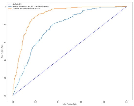
Figure 1.
ROC curves comparison.
Figure 1 shows the better predictive performance of the XGBoost method over the logistic regression. Indeed, the Area Under the Curve is 0.7715 for the logistic regression models and 0.9018 for the XGBoost model.
We now interpret the output of the XGBoost method by means of the SHAP values approach, for each explanatory feature available. This can be done with the TreeSHAP implementation, whose computational complexity reduces from to , where T is the number of trees, L is the maximum number of leaves in a tree, and D the maximal depth of a tree. Figure 2, below, contains the SHAP summary plot from TreeSHAP, which shows the contribution of each variable by representing its Shapley value averaged across all customers. In the figure, all of the observations are plotted row wise, separately for each explanatory variable. In each row, the color indicates the magnitude of each observation in terms of that variable: from low (blue color) to high (red color).
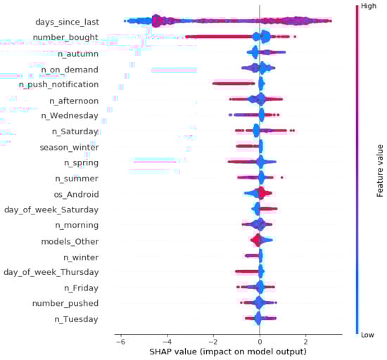
Figure 2.
Shapley Additive exPlanation (SHAP) summary plot.
From Figure 2, note that the most important variable to predict propensity to buy is the number of days since the last buy, followed by the number of bought items. In both cases, the impact on model output varies considerably among all of the observations (days since last), and especially for those with large values (number of bought items. Also note the effects of seasonality, in terms of weekdays and seasons. You can find a complete description of the variables used in Appendix A.
The third part of the analysis involves using the shap values vectors that correspond to each user, calculated from the classification model, and look for the presence of clustering structures that group together similar potential buyers. To this aim, we employ a K-means clustering algorithm Bindra and Mishra (2017). We have obtained that the optimal number of clusters is four by plotting the resulting within sum of squares against the number of clusters.
Thus, in Figure 3 we plot the scatterplot of the first two principal components of the SHAP values, attributing each consumer to one of the four clusters. In the Figure, the four cluster means are indicated with bolder nodes and positive events (consumers that buy) are coloured in red.
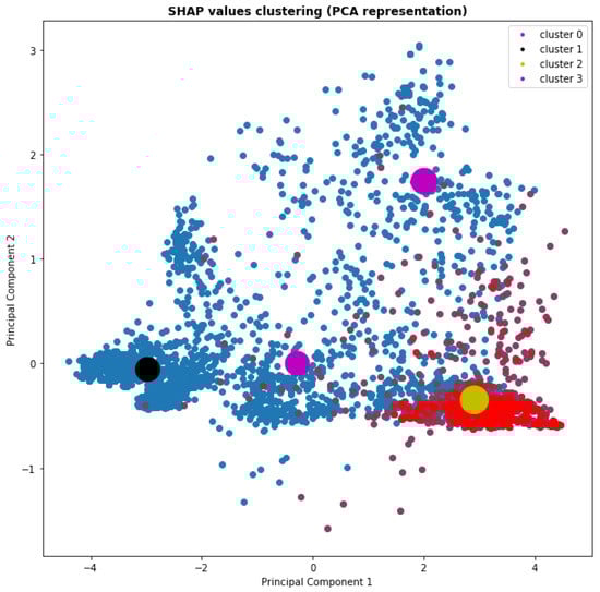
Figure 3.
Clustering of Shapley values.
From Figure 3, it can be noticed that one cluster is positioned in an area with virtually no red points (the black centroid), the two purple centroids are somewhat in-between and the cluster denoted by the yellow centroid is in an area with a high-density of propensity to buy users. Checking the proportion of positives with respect to each cluster, it turns out that the black cluster scores a 0.002 proportion (among the 1518 units that are contained in the cluster), the two purple clusters 0.09 and 0.093 (with 314 and 546 units in the clusters, respectively), while the yellow one shows a much larger 0.701, with 1400 units in the cluster.
It seems reasonable to group the two intermediate clusters into a new one, leaving us with three final clusters. In this way, we operate an effective segmentation among users, with a probability of buying ranging from 0.02% to 9% to 70%. The three clusters can be labeled, respectively, “unlikely”, “less likely”, and “very likely”.
The obtained results are consistent with what could be obtained when directly applying the K-means algorithm on the data, before XGboost and SHAP. In this case, the three probabilities, for the same clusters of individuals, are: 6%, 34%, and 70%. This reveals, as expected, the improved discriminatory capacity of the SHAP-XGBoost model over a pure empirical model, which does not filter any noise.
In addition, it can be shown that the three clusters that are obtained from the application of our proposal are well balanced, as we have 1495 users in the “unlikely” cluster, 866 users in the “less likely” cluster, and 1417 in the “very likely” one. Conversely, if we apply the K-mean clustering to the raw data, then we obtain a cluster of 951 units, with a 0.0641 proportion of events; two similar clusters with cumulatively 2807 units and a proportion of events of about 0.34 and a cluster with only 20 units and a 0.7 proportion: a rather unbalanced result. This further shows the advanage of our proposal, not only in terms of predictive accuracy and interpretability, but also in terms of cluster profiling.
In a similar fashion, we can apply our proposal for the customer churn problem. The AUROC value is equal to 0.91 against 0.75 for the selected stepwise logistic regression model. The application of the K-means clustering to the SHAP values leads to clusters being better separated than in the buying behaviour case, as shown in Figure 4, below.
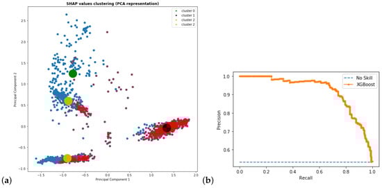
Figure 4.
(a) Clustering of Shapley values with K = 4; (b) Propensity to buy: Precision/Recall curve (Area Under the ROC Curve = 0.91).
Figure 4 shows a clear separation in four clusters, which can be again reduced to three, combining clusters 1 and 2. This leads to 222 users in the “unlikely” cluster, 803 in the “less likely”, and 664 in the “very likely” one. We summarize the three clusters, reporting the proportion of y and mean propensity for each cluster in Table 1.

Table 1.
Mean by cluster.
We finally remark that, also for this case, we have compared the K-means results over the SHAP vaues with the K-means results over the raw data and, again, the obtained clusters are better differentiated and balanced in the former case, confirming the advantage of using our proposed method.
3.3. Conclusions
In order to improve non-life insurance understanding of consumers’ need, we have proposed a novel methodology that can be embedded within a technological insurance service (Insurtech). The methodology, which is based on the combination of a highly accurate predictive method (XGBoost) with a model agnostic interpretability tool (Shapley Values), leads to a powerful segmentation of customer’s profiles, both in terms of buy and churn behaviours.
Our approach brings several advantages and, in particular, the ability to perform behavioural segmentation that is based on the behavioural similarity existing between customers. The research suggests that explainable machine learning models can effectively improve our understanding of customers’ behaviour. To further investigate this claim, future research may involve the application of the model to other situations that arise in the insurance industry, which may gain from the application of artificial intelligence technologies, such as underwriting and claims management.
Our approach can also be extended to other financial technology applications, such as peer-to-peer lending (Bussmann et al. 2020) and financial pricing (Giudici and Raffinetti 2020).
Another line of research would be to extend our approach when considering the Mean Absolute Shapley Values instead of the SHAP values, as in (Lundberg et al. 2020).
Author Contributions
The paper is a close collaboration between the two Authors. However, P.G. provided the concept and supervised; while A.G. coded and applied the methodology to the data. All authors have read and agreed to the published version of the manuscript.
Funding
This research has received funding from the European Union’s Horizon 2020 research and innovation program “FIN-TECH: A Financial supervision and Technology compliance training programme” under the grant agreement No 825215 (Topic: ICT-35-2018, Type of action: CSA).
Acknowledgments
We thank Pietro Menghi and the Neosurance team for useful comments and discussions. Finally, we acknowledgments go to the anonymous reviewers for their valuable comments and suggestions which allowed to improve the paper.
Conflicts of Interest
The authors declare no conflict of interest.
Appendix A
Table A1.
Variables’ description.
Table A1.
Variables’ description.
| Variable Name | Description |
|---|---|
| day_of_week | The weekday of the event |
| days_since_last | Days passed since last interaction with user |
| device | Type of device |
| models | Device model |
| models_Other | Catch-all label for low frequency device models |
| month | Month where the event occurs |
| n_afternoon | Cumulative number of interactions occurred this moment of the day |
| n_autumn | Cumulative number of interactions occurred this season |
| n_Friday | Cumulative number of interactions occurred this day |
| n_morning | Cumulative number of interactions occurred this moment of the day |
| n_on_demand | Cumulative number of requested policy quotes |
| n_push_notification | Cumulative number of notification pushed on device |
| n_Saturday | Cumulative number of interactions occurred this day |
| n_spring | Cumulative number of interactions occurred this season |
| n_summer | Cumulative number of interactions occurred this season |
| n_Tuesady | Cumulative number of interactions occurred this day |
| n_Wednesday | Cumulative number of interactions occurred this day |
| n_winter | Cumulative number of interactions occurred this season |
| number_bought | Number of bought policies |
| number_pushed | Number of times the insurance quote has been sent |
| os_Android | Flag to represent device OS Android |
| os_iOS | Flag to represent device OS iOS |
| season | Season where the event occurs |
| time_of_day | Moment of the day where the event occurs |
References
- Bernardino, Gabriel. 2020. Challenges and opportunities for the insurance sector. Annales des Mines, 99–102. [Google Scholar] [CrossRef]
- Bindra, Kamalpreet, and Anuranjan Mishra. 2017. A detailed study of clustering algorithms. Paper presented at 2017 6th International Conference on Reliability, Infocom Technologies and Optimization (Trends and Future Directions) (ICRITO), Noida, India, September 20–22; pp. 371–76. [Google Scholar]
- Breiman, Leo. 2000. Bias, Variance, and Arcing Classifiers. Technical Report 460. Oakland: Statistics Department, University of California. [Google Scholar]
- Bussmann, Niklas, Paolo Giudici, Dimitri Marinelli, and Jochen Papenbrock. 2020. Explainable machine learning in credit risk mamagement. Computational Economics. [Google Scholar] [CrossRef]
- Chen, Tianqi, and Carlos Guestrin. 2016. Xgboost: A scalable tree boosting system. Paper presented at 22nd ACM Sigkdd International Conference on Knowledge Discovery and Data Mining, San Francisco, CA, USA, August 13–17; pp. 785–94. [Google Scholar] [CrossRef]
- European Commission. 2020. On Artificial Intelligence—A European Approach to Excellence and Trust. Brussels: European Commission. [Google Scholar]
- Giudici, Paolo, and Emanuela Raffinetti. 2020. Shapley-Lorenz eXplainable artificial intelligence. Expert systems with applications. Expert Systems with Applications. [Google Scholar] [CrossRef]
- Guidotti, Riccardo, Anna Monreale, Franco Turini, Dino Pedreschi, and Fosca Giannotti. 2018. A survey of methods for explaining black box models. arXiv arXiv:1802.01933. [Google Scholar] [CrossRef]
- Joseph, Andreas. 2019. Shapley regressions: A framework for statistical inference on machine learning models. arXiv arXiv:1903.04209. [Google Scholar]
- Lundberg, Scott M., and Su-In Lee. 2017. A unified approach to interpreting model predictions. In Advances in Neural Information Processing Systems. Cambridge: The MIT Press. [Google Scholar]
- Lundberg, Scott, Gabriel Erion, and Su-In Lee. 2018. Consistent individualized feature attribution for tree ensembles. arXiv arXiv:1802.03888. [Google Scholar]
- Lundberg, Scott M., Gabriel Erion, Hugh Chen, Alex DeGrave, Jordan M. Prutkin, Bala Nair, Ronit Katz, Jonathan Himmelfarb, Nisha Bansal, and Su-In Lee. 2020. From local explanations to global understanding with explainable ai for trees. Nature Machine Learning 2: 2500–5839. [Google Scholar] [CrossRef] [PubMed]
- MacQueen, James. 1967. Some Methods for Classification and Analysis of Multivariate Observations. Proceedings of the Fifth Berkeley Symposium on Mathematical Statistics and Probability. pp. 281–97. Available online: https://projecteuclid.org/euclid.bsmsp/1200512992 (accessed on 6 November 2020).
- Molnar, Christoph. 2019. Interpretable Machine Learning. Available online: https://christophm.github.io/interpretable-ml-book/ (accessed on 21 September 2020).
- Murdoch, W. James, Chandan Singh, Karl Kumbier, Reza Abbasi-Asl, and Bin Yu. 2019. Interpretable machine learning: Definitions, methods, and applications. arXiv arXiv:1901.04592. [Google Scholar] [CrossRef] [PubMed]
- Shapley, Lloyd S. 1952. A Value for N-Person Games; Fairfax: Defense Technical Information Center.
- Strumbelj, Erik, and Igor Kononenko. 2010. An efficient explanation of individual classifications using game theory. The Journal of Machine Learning Research 11: 1–18. [Google Scholar]
Publisher’s Note: MDPI stays neutral with regard to jurisdictional claims in published maps and institutional affiliations. |
© 2020 by the authors. Licensee MDPI, Basel, Switzerland. This article is an open access article distributed under the terms and conditions of the Creative Commons Attribution (CC BY) license (http://creativecommons.org/licenses/by/4.0/).