Article

Comparing Two Different Option Pricing Methods

by
Alessandro Bondi
1,
Dragana Radojičić
2,* and
Thorsten Rheinländer
2
1
Classe di Scienze, Scuola Normale Superiore di Pisa, 56126 Pisa, Italy
2
TU Wien, Institute of Statistics and Mathematical Methods in Economics, 22180 Vienna, Austria
*
Author to whom correspondence should be addressed.
Risks 2020, 8(4), 108; https://doi.org/10.3390/risks8040108
Submission received: 4 September 2020 / Revised: 12 October 2020 / Accepted: 14 October 2020 / Published: 19 October 2020
(This article belongs to the Special Issue Interplay between Financial and Actuarial Mathematics)

Abstract

:
Motivated by new financial markets where there is no canonical choice of a risk-neutral measure, we compared two different methods for pricing options: calibration with an entropic penalty term and valuation by the Esscher measure. The main aim of this paper is to contrast the outcomes of those two methods with real-traded call option prices in a liquid market like NASDAQ stock exchange, using data referring to the period 2019–2020. Although the Esscher measure method slightly underperforms the calibration method in terms of absolute values of the percentage difference between real and model prices, it could be the only feasible choice if there are not many liquidly traded derivatives in the market.

1. Introduction

Empirical studies show that real financial markets are incomplete, which means that not all derivative securities like options are replicable by means of some initial capital plus the value process of some self-finance trading strategy, and therefore hold unhedgeable and undiversifiable risks. The second fundamental theorem of asset pricing implies that in incomplete markets there typically exist several martingale measures consistent with the no-arbitrage principle that can be chosen as pricing measures (see, e.g., Jeanblanc et al. 2009; Shreve 2004). In fact, the range of option prices composes the total range between the inf and the sup of expected values with respect to martingale measures, and is therefore too large for practical purposes, see (Eberlein and Hammerstein 2004, Theorem 11.55).
Therefore, it makes sense to select a particular martingale measure for pricing purposes. In this study, we introduce, discuss, and compare two methods for the simulation of European call option prices: one based on the Esscher martingale measure and the other on the calibration to real-traded securities with an entropic penalty term. We implemented them in the programming language R and contrast the simulated derivative prices with real data retrieved from NASDAQ option chains. The objective of the paper was to provide a good fit between real and simulated contingent claim prices, consequently suggesting a choice for risk-neutral pricing measures in incomplete markets. In order to fulfill this aim, we constructed a model rich enough to describe stock prices but feasible for practice and connected to option prices. In this context, it is natural to exogenously specify different, suitable underlying asset price dynamics on a case-by-case basis.
The Esscher transform, invented by the Swedish actuary F. Esscher and introduced in Esscher (1932), is a time-honored tool in actuarial science for approximating the distribution of the aggregate claims of a portfolio. It consists of an exponential tilting procedure. More recently, it has been used as a premium calculation principle, see Van Heerwaarden et al. (1989), in option pricing, see Gerber and Shiu (1994), and also in pricing defaultable assets, see Lee and Rheinländer (2012). In our financial setting, the agent has the option to invest in a financial market via admissible strategies. Hereby we exclude strategies leading to arbitrage opportunities. The corresponding theory has been developed by Kallsen and Shiryaev, see Kallsen and Shiryaev (2002). In Benth and Schmeck (2014), the authors used an Esscher transform incorporated in a two-factor model to derive futures prices in electricity markets. Furthermore, pricing methodology for weather derivatives in a specific two-factor model is established in Hell et al. (2012).
The idea of calibration is to consider a set of liquid option prices, and to find a market martingale measure such that the expected values of the option payoffs are as close as possible to the observed prices. This approximation problem is typically ill-posed, and one has to include a regularization term, we opted for an entropic penalty term in this regard. A general exposition about the calibration method can be found in Cont and Tankov, see Cont and Tankov (2004a).
Section 2 and Section 3 are divided into a theoretical and a numerical part. The second section is devoted to the geometric Esscher measure and Laplace cumulant processes. In this part, we modeled the log–prices of the stock with a C O G A R C H process (introduced in Klüppelberg et al. (2004)) and present a sufficient condition for the existence of such a measure. Assuming the driving Lévy process to have a N I G (normal inverse Gaussian) distribution, which is infinitely divisible and thus corresponds to a Lévy process, we explain the original procedure—relying on the canonical representation theorem for semimartingales—followed by simulating the paths of the stock pricesunder the martingale measure. We pinpoint that, as Lemma 1 shows, the choice of the N I G distribution in the C O G A R C H model is crucial, since it allows for generating the risk-neutral trajectories of the underlying asset price.
In the third section, the calibration method is explained; using the fundamental concepts of relative entropy of distributions and Lévy processes on the Skorohod space (presented in Appendix E), we chose a martingale measure under which the dynamics of the stock prices follow an exponential Lévy process. In this part we mainly follow Cont and Tankov (2004a), even if the mathematical structure was refined and generalized, and the numerical approximation machinery was tailored to our goals.
In order to make the readers familiar with the theory and the notation that stands behind the main concepts of these two methods, in the appendix we also present a construction of the N I G distribution and some essential results on Lévy processes, highlighting the connection with the characteristics of semimartingales.
The main point of the present paper is as follows: if there are many liquid options around, like plain vanilla calls and puts on liquid stocks, we would expect the calibration method to perform best, therefore, we chose it as the benchmark method. However, in new financial markets, like insurance derivatives, cryptocurrencies, energy, or electricity markets, there are often only a few derivatives or any at all available, or the underlying (like electricity) is difficult to trade in since it is not storable. In these cases the calibration method is not implementable, and there is not much choice other than to use the Esscher method which has been done, e.g., in the book by Benth, Benth, and Koekebakker about electricity and related markets, see Benth et al. (2008). Besides that, there are few, if at all, studies about practical implementation of hedging strategies in incomplete markets, therefore our study fills a gap in this direction. Our main result thus is that while the Esscher martingale measure based pricing method in a liquid market does underperform the calibration method, as is to be expected, it does so only by less than 5%. So it might be a feasible choice of method in new financial markets.

2. Esscher Measure Method

In this section, the dynamics of the stock prices are introduced and sufficient conditions for the existence of the Esscher measure, which was used to simulate European call options prices, are established. We refer to Appendix D for a brief summary of the theory, which is necessary to construct the geometric Esscher measure. In the following, we use notation that can be found, e.g., in the books (Rheinländer and Sexton 2011; Shiryaev and Jacod 2003), as well as references therein.

2.1. The Model

On a probability space Ω , F , P we introduce a driving, R -valued Lévy process L = L t t with generating triplet σ 2 , ν , γ h with respect to a truncation function h (see Appendix B and Appendix C). We endow this space with F , the augmented filtration of L. Define the dynamics of the spot prices by the process S = S t t , where S : = S 0 exp G , S 0 R + , with the log-prices G = G t t which follow a C O G A R C H process, introduced in Klüppelberg et al. (2004):
d G t = σ t d L t , G 0 = 0 .
The volatility process σ 2 = σ t 2 t is given by
σ t 2 : = k 0 t e X s d s + σ 0 2 e X t , t 0 ,
with σ 0 2 R + and an adapted, right-continuous with left limits (RCLL) process X = X t t defined by
X t : = η log δ 0 < s t log 1 + Φ Δ L s 2 , t 0 ,
where k > 0 , η > 0 , Φ 0 . We recall that a process is said to be RCLL if it has, almost surely, right-continuous trajectories with left limits. Although σ 2 is a left-continuous process, as shown by (2), we use σ with the aim to highlight that we are working with a process which is adapted and left-continuous, therefore predictable.
For an adapted process r = r t t modeling the interest rate, the discounted spot price process is given by S ˜ = S ˜ t t , where S ˜ t : = exp 0 t r s d s S t , t 0 . Thus, we consider the process G = G t t , where G t : = 0 t r s d s + G t for every t 0 , whose dynamics follow d G t = r t d t + d G t . At this point, we can express S ˜ = S 0 exp G and we want to find a process θ L G such that S ˜ is a P θ –local martingale: P θ denotes the geometric Esscher measure, or Esscher martingale transform, for the exponential process S ˜ (see Appendix D).
Remark 1.
From (1), it is clear that G jumps at the same times as L does, and Δ G t = σ t Δ L t for every t 0 . For t R + and ω Ω , the measure associated with its jumps is
μ G ω ; 0 , t × A = s t 1 x 0 A Δ G s ( ω ) = s t 1 x 0 Δ L s ω 1 σ s ω 1 A Δ L s ω = μ L ω ; 0 , t × σ ω 1 A , A B R .
Furthermore μ G = μ G , hence F t , ω G d y = ν σ t ω · 1 d y , meaning that
F t , ω G A = R 1 A σ t ω y ν d y , A B R .
Theorem 1.
Let θ L ( G ) be such that θ · G is exponentially special and Z θ is a uniformly integrable martingale. If also θ + 1 · G is exponentially special and θ satisfies
θ t + 1 2 σ t 2 σ 2 r t + σ t γ h + R e θ t + 1 σ t y e θ t σ t y σ t h y ν d y = 0
for every t 0 , then S ˜ is a P θ -local martingale.
Note that G is a 1-dimensional process, thus the geometric Esscher measure is unique.
Proof. 
Let
G ˜ h t : = s t Δ G s h Δ G s = x h x 🟉 μ G t , t 0
and G h t : = G t G ˜ h t , t 0 . By Remark 1, we get
d G h t = d G t d G ˜ h t = r t d t + d G t x h x μ G d t , d x = r t d t + σ t d L t σ t y h σ t y μ L d t , d y .
Taking into account Lemma A1 in Appendix D, which provides
δ L σ t = σ t γ h + R σ t y h y ν ( d y ) , t 0 ,
and considering that σ · L c = σ · L c and σ · L c , σ · L c = σ 2 σ 2 d t , we obtain the characteristics of G under P with respect to h:
b t G = r t + σ t γ h + R h σ t y σ t h y ν ( d y ) c t G = σ t 2 σ 2 F t G ( d y ) = ν ( σ t · ) 1 d y , t 0 .
Thus, if θ satisfies κ ˜ θ + 1 κ ˜ θ = 0 , thanks to Theorem A2 we can conclude that S ˜ is a P θ -local martingale. In fact, using (A11) we have
κ ˜ θ + 1 t κ ˜ θ t = b t G + 1 2 σ t 2 σ 2 + θ t σ t 2 σ 2 + R e θ t + 1 x e θ t x h x F t G ( d x ) = θ t + 1 2 σ t 2 σ 2 r t + σ t γ h + R e θ t + 1 σ t y e θ t σ t y σ t h y ν d y = 0 , t 0 ,
where the last equality holds by (3). □
The next lemma provides us with the candidate solutions to Equation (3) when L follows a N I G distribution (see Appendix A).
Lemma 1.
Let L = L t t be a N I G -distributed Lévy process with parameters α , β , μ , δ and define the truncation function h x : = x 1 D x , x R . If a process θ = θ t t such that
σ t θ t ω , σ t θ t + 1 ω α β , α β , t R 0 + , ω Ω
fulfills Equation (3), then for every t 0 we have
θ t 1 , 2 = 1 2 R t 2 + δ 2 σ t 2 σ t ( δ 2 σ t 3 2 β δ 2 σ t 2 R t 2 σ t + 2 β ± 4 α 2 δ 2 R t 2 σ t 2 + 4 R t 4 α 2 R t 2 δ 2 σ t 4 R t 6 δ 2 2 σ t 2 R t 4 ) ,
with R t : = r t + μ σ t .
Proof. 
Since L 1 N I G α , β , μ , δ , we apply (A6) and (A9) (see Appendix A and Appendix B) to obtain
E e z L 1 = exp μ z + γ 1 z + R e z x 1 z x 1 D x ν d x , z α β , α β ,
where γ 1 : = 2 δ α π 0 1 sinh β x K 1 α x d x and ν d x = δ α π x e β x K 1 α x d x . Using (A5), we get
δ α 2 β 2 α 2 β + z 2 = γ 1 z + R e z x 1 z x 1 D x ν d x
for z α β , α β . Proceeding as in the proof of Theorem 1, we have
0 = κ ˜ θ + 1 t κ ˜ θ t = R t + σ t γ 1 + R e θ t + 1 σ t x 1 σ t θ t + 1 x 1 D x ν d x R e θ t σ t x 1 σ t θ t x 1 D x ν d x , t 0 .
Since σ γ 1 = σ θ + 1 θ γ 1 , we expand on the chain of equalities in (8):
0 = R t + σ t θ t + 1 γ 1 + R e θ t + 1 σ t x 1 σ t θ t + 1 x 1 D x ν d x σ t θ t γ 1 + R e θ t σ t x 1 σ t θ t x 1 D x ν d x = R t + δ α 2 β + σ t θ t 2 α 2 β + σ t θ t + 1 2 , t 0 ,
where the last equality is obtained by combining (5) and (7). At this point it remains to find the possible solutions for every t 0 to the equation
R t + δ α 2 β + σ t θ t 2 α 2 β + σ t θ t + 1 2 = 0 ,
which can be written as α 2 β + σ t θ t + 1 2 = R t δ + α 2 β + σ t θ t 2 . Squaring both sides we get
2 R t δ α 2 β + σ t θ t 2 = σ t 2 + 2 β σ t + R t 2 δ 2 2 σ t 2 θ t ,
and repeating once again the same operation of squaring we end up with an equation of second degree in θ :
4 σ t 2 σ t 2 + R t 2 δ 2 θ t 2 + 4 σ t σ t 3 + 2 β σ t 2 + R t 2 δ 2 σ t + 2 β R t 2 δ 2 θ t + c t = 0 ,
where c t : = σ t 2 + 2 β σ t + R t 2 δ 2 2 4 R t 2 δ 2 α 2 β 2 . Computing algebraically the solutions of (10) we get the expressions in (6). □
We have empirically tested both possible branches of solutions in (6), and we have chosen
θ t = 1 2 R t 2 + δ 2 σ t 2 σ t ( δ 2 σ t 3 2 β δ 2 σ t 2 R t 2 σ t + 2 β 4 α 2 δ 2 R t 2 σ t 2 + 4 R t 4 α 2 R t 2 δ 2 σ t 4 R t 6 δ 2 2 σ t 2 R t 4 )
to run the simulation because it prevents the risk-neutral dynamics from “exploding”, i.e., from skyrocketing to unrealistically high prices in a short time.
Remark 2.
Unfortunately, it does not seem possible for us to prove, from an analytical point of view, that either candidate solution in (6) solves (3), i.e., that it is a true solution. What the simulations suggest is that only the process in (11) is indeed a solution of (3). This insight is confirmed by the numerical experiments to a greater extent. In fact, it turns out that both processes θ 1 , 2 satisfy Condition (5). However, θ 1 makes the right hand side in (9) negative, and this implies that it does not solve (3). On the contrary, the process θ 2 —the one we pick in (11)—makes such term positive, hence it solves (3), indeed.

2.1.1. Simulation of the P θ -Dynamics

The goal of this section is to carefully describe a procedure to generate the risk-neutral dynamics of the underlying asset price. This allows us to compute the simulated European call option prices with the Monte Carlo method.
Let r R + represent the constant annual interest rate. We assume that the driving Lévy process L is N I G -distributed and that the hypothesis of Theorem 1 hold (with respect to the truncation function h ¯ x = x 1 D x , x R ). Using the R-package yuima (see Iacus 2011) we estimate the parameters of the model from the time series of the underlying asset log-prices. Next, we simulated a sufficiently large number of paths of the variance process σ 2 with the found parameters: by (11), from each of them we can get a trajectory of θ . The issue reduces to generating the paths of G, but note that, after the change of measure, L is not a Lévy process anymore because F t θ d x = e θ t x ν d x , t 0 . Consequently, G is not a C O G A R C H process under the martingale measure. Then, in order to simulate its trajectories we use the canonical representation for semimartingales (Shiryaev and Jacod (2003), Chapter II, Theorem 2.34): for a d-dimensional semimartingale X = X t t with characteristics B , C , ν X relative to the truncation function h, it holds:
X = X 0 + X c + B + h x 🟉 ( μ X ν X ) + x h x 🟉 μ X .
The symbol 🟉 denotes the integration with respect to a random measure: we refer to (Shiryaev and Jacod (2003), Chapter II, Section 1) for an extensive study of this topic. For the reader’s convenience, we provide the basic definition.
Definition 1.
Let μ be a random measure on R 0 + × R and W : Ω × R 0 + × R R be measurable function with respect to the product σ-algebra O B R , where O denotes the optional σ-algebra on Ω × R 0 + . The integral process W 🟉 μ is defined by
W 🟉 μ t ω : = 0 , t × R W ω ; s , x μ ω ; d s , d x , if 0 , t × R W ω ; s , x μ ω ; d s , d x < , otherwise .
For an arbitrarily chosen ϵ 1 , fix the truncation function h x : = x 1 z < ϵ x for x R , and let 0 , ν , γ h be the corresponding generating triplet of L. From the proof of Theorem 1, specifically from (4), we readily get the characteristics b t , 0 , ν σ t · 1 d x of G under P, and invoking (A12) and Remark A2 in Appendix D we find them under P θ :
b t θ = b t + R h x e θ t x 1 F t ( d x ) c t θ = 0 F t θ ( d x ) = e θ t x ν ( σ t · ) 1 d x , t 0 .
We now represent G by (12), noting that G 0 = 0 and G c = 0 since c θ = 0 . As regards the term B = B t t , we expand on the computations in (13), getting
b t θ = σ t γ h + x < ϵ / σ t σ t y δ α π y e θ t σ t + β y K 1 α y d y ϵ , ϵ σ t y δ α π y e β y K 1 α y d y , t 0 ,
and obtain the variables of the process B by B t = 0 , t b s θ d s , t 0 .
At this point we need to approximate a trajectory of the process h x 🟉 ( μ G ν G ) . In order to do so, we neglect the contribution of the jumps of G with absolute value smaller than ϵ , focusing just on the term
h x 🟉 ( μ G ν G ) h x 🟉 ν G = 0 , t d s R x 1 z < ϵ x F s θ d x = 0 , t d s x < ϵ / σ s σ s y δ α π y e θ s σ s + β y K 1 α y d y , t 0 ,
which in turn cancels out with one of the addends defining B. Heuristically speaking, in this approach we are assuming that the small jumps of the underlying asset price do not contribute to the determination of the option value in a significant way. However, we may refer to Asmussen and Rosiński (2001) for a more sophisticated procedure taking into account the variation of such small jumps in the case of Lévy processes.
Finally we concentrate on the term x h x 🟉 μ G : we simulate its paths similarly to the Lévy–Itô decomposition theorem (see Sato 1999, Theorem 19.2). According to this result, if L ˜ is a Lévy process with generating triplet A , ν , γ and D a , : = x R d : a < x < for a > 0 , then x x 1 D x 🟉 μ L ˜ t t is a compound Poisson process with constant ν D 1 , and distribution
ϕ B : = 0 , if B D ν B D 1 , ν D 1 , , otherwise , B B R d .
Thus, we take a nonhomogeneous Poisson process with time-varying intensity
λ t : = F t θ x > ϵ = R e θ t σ t y 1 D ϵ , σ t y δ α π y e β y K 1 α y d y = x > ϵ / σ t δ α π y e θ t σ t + β y K 1 α y d y , t 0
and impose the time-varying jumps sizes to follow
c t : = R x 1 D ϵ , x λ t F t θ d x = 1 λ t x > ϵ / σ t σ t y δ α π y e θ t σ t + β y K 1 α y d y , t 0 .
The jump times of this process have been simulated by the thinning algorithm described in Lewis and Shedler (1979).
Denote by N the number of iterations we run and by S i , for i = 1 , , N , the corresponding, simulated trajectories of the spot price under the pricing measure P θ . We obtain the value of an European call option with strike K and maturity T following the Monte Carlo method, i.e., computing the sample mean of the vector of components e r T S i T K + , i = 1 , , N .

2.1.2. Empirical Results

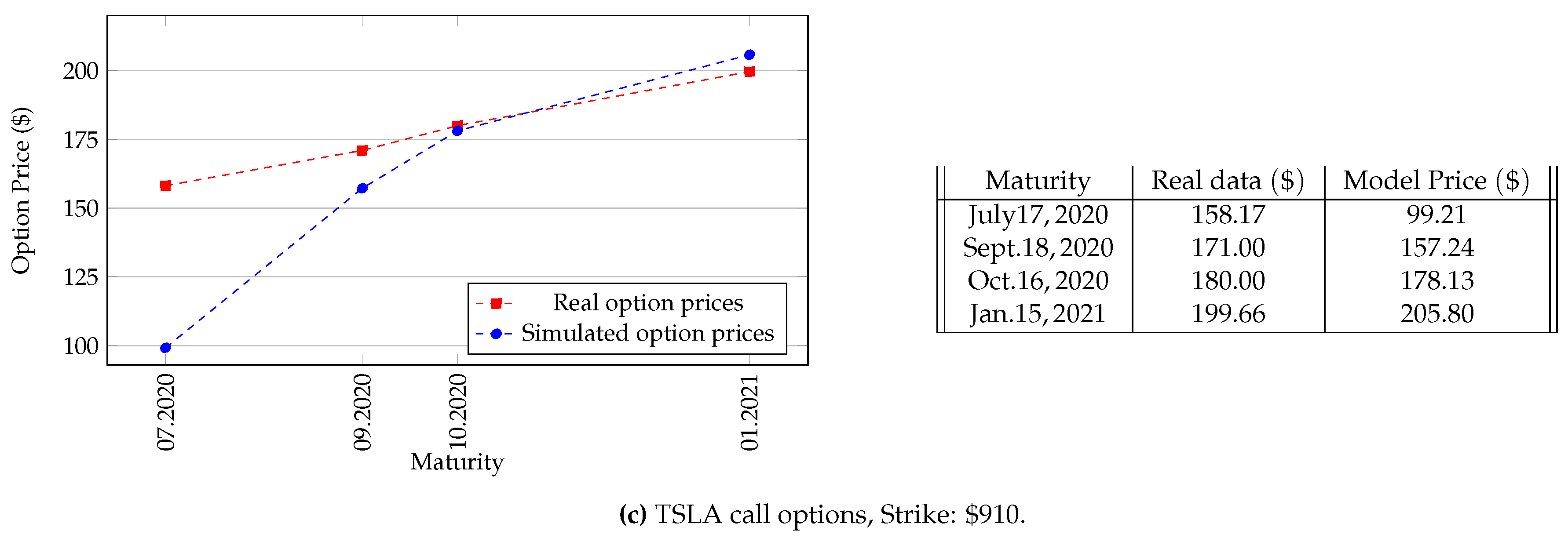
We have empirically tested the Esscher method on the prices of call options on Apple Inc. stock (ticker symbol: AAPL) with fixed strike at $ 320 . In Figure 1a, the simulated option prices are shown as function of their maturities. The average of the absolute values of percentage difference is 3.1646 % .
Furthermore, we applied this method to the prices of call options on Microsoft Corporation stock (ticker symbol: MSFT) with strike $ 190 : we plot the outcomes in Figure 1b. In this case, the mean of absolute values of percentage difference settles down at 5.0518 % .
Finally we report the results of a test on call options with strike $ 910 with Tesla, Inc. (ticker symbol: TSLA) as underlying stock. In Figure 1c we can notice a big discrepancy between the real price and the predicted value for the shortest-term maturity taken into account, the latter being 37.2755 % smaller than the former. However, if we neglect this first term we recover a result in line with the previous experiments, namely an average for the absolute values of percentage difference of 4.0555 % .
In all the three cases, we set the number of Monte Carlo iterations N = 10 4 and we used the time series of the log prices associated to the trading year before 19 February 2020, to estimate the parameters of the C O G A R C H model (see Section 2.1.1). Therefore, the simulations were run prior to Apple’s stock split (on 28 August 2020) and Tesla’s stock split (on 31 August 2020).
Remark 3.
The real data was obtained from https://old.nasdaq.com, where American options are traded. Although our approximation generates the prices in an European model, it can be accepted as meaningful since:
  • the analyzed derivatives have short-term maturities, so we are allowed to ignore the dividend yield (however, TSLA does not pay dividends);
  • the time values of the options were always positive, implying that it is convenient to sell the option rather than exercising the call right.

3. Calibration with Entropic Penalty Term Method

In the Esscher method, the density process is completely defined by the spot prices: this is an intuitive drawback in liquid markets, because it does not use all the available information (e.g., the time series of derivative prices). This is a motivation to consider the Calibration Method, which consists in modeling the spot prices dynamics directly under a martingale measure “chosen” by the market.

3.1. The Model

We start the practical analysis by taking into account a driving, R -valued Lévy process L = L t t with generating triplet σ 2 , ν , γ on a probability space Ω , F , Q endowed with the augmented filtration of L, which satisfies the usual conditions and is denoted by G . We describe the stock prices S = S t t with an exponential Lévy model: S t : = S 0 exp r t + L t , t 0 , with S 0 R + and r R + representing the constant annual interest rate. The discounting process R = R t t reduces to the deterministic function R t : = exp r t , t 0 . Since we need Q to be a martingale measure for S we require:
(i)
there exists a t > 0 such that E Q [ exp L t ] < ;
(ii)
Ψ 1 = 1 2 σ 2 + γ + R e x 1 x 1 D x ν d x = 0 .
With these assumptions, Remark A1 in Appendix B proves that exp L t t is a martingale with E Q exp L t = 1 for every t > 0 . Considering the discounted spot prices process S ˜ = S ˜ t t , defined by S ˜ t : = R t S t = S 0 exp L t , t 0 , we can state that it is a Q-martingale with constant expectation equal to S 0 .
In our discussion the driving Lévy process L will be a pure jump process, so its generating triplet simplifies as σ 2 = 0 . In particular, due to assumption (ii) we get the next relation:
γ = R e x 1 x 1 D x ν d x .
Assume that there are N European call options with fixed maturity T available in the market, and for each j = 1 , , N let K j and C j be the strike price and the observed price of the j-th derivative, respectively. It is convenient to consider the quantities k j = log K j , j = 1 , , N . In this setting, S is the price process of the underlying asset. Since Q is a martingale measure for S, we can use it to price options: C ν j : = exp r T E Q S T exp k j + , j = 1 , , N . Denoting by Q L T the pushforward distribution on R generated by L T we have
C ν j = exp r T R S 0 e r T + y e k j + Q L T d y , j = 1 , , N .
Thus, knowing the Lévy measure ν , the whole generating triplet could be recovered and therefore the option prices computed.
The reasoning which leads the calibration is choosing ν such that C ν j is “close” to C j for any j = 1 , , N . Hence we pick the Lévy measure of the model by a least-squares procedure:
ν ¯ = arg min ν j = 1 N C ν j C j 2 .
Since the problem expressed in (15) is ill posed (see Cont and Tankov 2004a, Chp. 13), we introduce a regularization term. Let L 0 = L t 0 t be a, pure jump, driving Lévy process with generating triplet 0 , ν 0 , γ 0 statistically estimated from the time series of the underlying asset price. Furthermore, let Q L 0 and Q L be the distributions on the Skorohod space D , F D ; F generated by L 0 and L, respectively, which are supposed to be equivalent on F t for every t > 0 (see Appendix E). We use the relative entropy as a measure of the distance from Q L 0 , so that by Remark A3 the issue is reduced to solving the optimization problem:
ν ¯ = arg min ν Q j = 1 N C ν j C j 2 + α R d ν d ν 0 log d ν d ν 0 + 1 d ν d ν 0 d ν 0 ,
for Q : = ν : Q L | F t Q L 0 | F t , t > 0 . The term α is a regularization parameter: the higher it is, the more we trust the initial distribution and the less importance we give to calibration. The existence of a solution to (16) has been studied, among others, in the paper Cont and Tankov (2004b). We are going to relax the assumptions in (16), considering the minimization in the set of the Lévy measures equivalent to ν 0 .

3.1.1. Numerical Approximation

The goal of this section is to describe in each and every detail a discretization procedure that allows us to tackle the optimization problem in (16). To this aim, it is necessary to express the objective functional in (16) as a function of the masses of the discretized Lévy measures. The steps of our argument are the following:
I.
estimate the parameters of the prior Lévy process L 0 from the time series of log–returns;
II.
introduce a discretization grid for the prior Lévy measure ν 0 and the driving Lévy measure ν (in what follows, the points of such a grid are denoted by y 1 < < y N d ). Their discretized versions are denoted by ν d 0 and ν d , respectively;
III.
compute the discrete version of the entropy term in (16) as a function of the masses of ν d ;
IV.
use an approach based on the Fourier inversion theorem to get an approximation of the modified time values of the options at the log–strikes under scrutiny. This allows us to obtain (23), a discretized version of the objective functional in (16);
V.
calculate explicitly the derivatives of the discretized objective functional to speed up the simulations;
VI.
choose the regularization parameter α .
Fix a maturity T and define the grid x j R + , j = 1 , , N , with x 1 < x 2 < < x N : these points represent the log–strike prices of the options available on the market. Moreover, from the time series of the log–returns we obtain the parameters of the historical, N I G -distributed Lévy process L 0 = L t 0 t by a maximum likelihood procedure using the R-package ghyp. Note that, in this case, one can select any pure jump, infinitely divisible distribution: we opt for the NIG by analogy with the Esscher’s method, and our choice is satisfactory, as the final goodness of fit between real data and model prices shows. First we introduce a discretization grid consisting in the points y h , h = 1 , , N d , with y 1 < y 2 < < y N d , which constitutes a partition of the interval M , M for some M > 0 , and then we approximate the Lévy measure of L 0 with the discrete version ν d 0 d y = h = 1 N d ν h 0 δ y h d y , where δ a ¯ denotes the Dirac measure at a point a ¯ and
ν 1 0 = , y 1 d ν 0 ; ν h 0 = y h 1 , y h d ν 0 , h = 2 , , N d 1 ; ν N d 0 = y N d 1 , d ν 0 .
Now we take into account another measure which has the same mass points as the previous one: ν d d y = h = 1 N d ν h δ y h d y , with ν h R + for every h = 1 , , N d . We note that the calibrated measures ν d and ν d 0 are equivalent, but ν d and the prior ν 0 are not. We understand the measure ν d as the discretized Lévy measure of the driving, pure jump Lévy processes L = L t t . We now want to compute the Radon–Nikodym derivative d ν d d ν d 0 with the aim to explicitly express the entropy term of (16) in the discrete version
R d ν d d ν d 0 log d ν d d ν d 0 + 1 d ν d d ν d 0 d ν d 0 .
Set y 0 = and define the function
f y : = ν h ν h 0 , if y h 1 < y y h , h = 1 , , N d 0 , otherwise .
For every A B R it results
R f 1 A d ν d 0 = h = 1 N d ν h ν h 0 y h 1 , y h 1 A y ν d 0 d y = h = 1 N d ν h ν h 0 ν d 0 y h 1 , y h A = h = 1 N d ν h ν h 0 ν h 0 1 A y h = ν d A ,
as ν d 0 y h 1 , y h A = ν h 0 1 A y h , h = 1 , , N d . Therefore, d ν d d ν d 0 = f . Moving back to the integral (17), we get:
R d ν d d ν d 0 log d ν d d ν d 0 + 1 d ν d d ν d 0 d ν d 0 = , y N d d ν d d ν d 0 log d ν d d ν d 0 + 1 d ν d d ν d 0 d ν d 0 = h = 1 N d ν h ν h 0 log ν h ν h 0 + 1 ν h ν h 0 ν d 0 y h 1 , y h = h = 1 N d ν h log ν h log ν h 0 + ν h 0 ν h .
Following the Carr and Madan approach (see Carr and Madan 1999, Section 3.2) for further details), we are able to to express the quantity j = 1 N C ν j C j 2 as a function of ν 1 , , ν N d . The option price C ν k is not an integrable function, as a swift application of Lebesgue’s convergence theorem shows that it converges to S 0 as k . Therefore, we focus on the modified time value z T , defined by z T k : = C ν k S 0 e k r T + , k R . We suppose that z T and its inverse Fourier transform ζ T are integrable, so by inversion (see, e.g., Rudin 1987, Theorem 9.11) we have
z T k = 1 2 π R e i k u ζ T u d u a . e .
Fix k R ; we first analyze the term
S 0 e k r T + = S 0 e k r T 1 z log S 0 + r T k = e r T R e log S 0 + r T e k 1 z log S 0 + r T k Q L T d y .
In a similar way we get
C ν k = e r T R e y + log S 0 + r T e k 1 z y + log S 0 + r T k Q L T d y .
This provides the following expression for z T k :
z T k = e r T R S 0 e r T + y e k 1 z k log S 0 r T y S 0 e r T e k 1 z log S 0 + r T k Q L T d y .
The assumption (ii) ensures that R e y Q L T d y = 1 , so we finally obtain
z T k = e r T R S 0 e r T + y e k 1 z k log S 0 r T y 1 z log S 0 + r T k Q L T d y , k R .
The insight here is to use the Fourier transform and its inverse to estimate the values z T x j for every j = 1 , , N . Hence we fix a point u R and introduce the inverse Fourier transform
ζ T u : = 1 2 π R e i u k z T k d k .
Under suitable conditions which allow us to switch the order of integration we have
ζ T u = e r T 2 π , 0 y + log S 0 + r T , log S 0 + r T e i u k S 0 e r T + y e k d k Q L T d y + e r T 2 π 0 , log S 0 + r T , y + log S 0 + r T e i u k S 0 e r T + y e k d k Q L T d y .
We turn our attention on the computation of the first term of the sum (19). An explicit calculation of the inner integral (respect to the Lebesgue measure) of such addend, indicated by I 1 , gives
I 1 y = S 0 e r T + y + i u log S 0 + r T i u ( i u + 1 ) i u 1 e y + 1 e i u y = S 0 e r T + i u log S 0 + r T i u + 1 e y 1 + S 0 e r T + i u log S 0 + r T i u i u + 1 e y S 0 e i u log S 0 e i u + 1 r T i u i u + 1 e y + i u y , y , 0 .
The same strategy allows us to compute the inner integral I 2 of the second addend in (19), as well. Precisely, for every y 0 , we get
I 2 y = S 0 e r T + i u log S 0 + r T i u + 1 e y 1 S 0 e r T + i u log S 0 + r T i u i u + 1 e y + S 0 e i u log S 0 e i u + 1 r T i u i u + 1 e y + i u y .
Therefore we are able to represent the inverse Fourier transform as
ζ T u = S 0 2 π e i u log S 0 + r T i u + 1 R 1 e y Q L T d y 1 i u R e y Q L T d y + 1 i u R e y + i u y Q L T d y .
Both (A9) in Appendix B and assumption (i) make us conclude that
ζ T u = S 0 2 π e i u log S 0 + r T i u i u + 1 e T Ψ i u + 1 1 , u R .
By the definition of Ψ in (A8) (see Appendix B), substituting the discrete version ν d for the Lévy measure ν associated to L, as a consequence of (14) we get, for every u R ,
Ψ i u + 1 R e i u + 1 y i u e y e y + i u ν d d y = h = 1 N d e y h e i u y h 1 ν h + i u h = 1 N d 1 e y h ν h .
Plugging (21) into (20) we obtain, for u R , the final approximation
ζ T u S 0 2 π e i u log S 0 + r T i u i u + 1 exp T h = 1 N d e y h e i u y h 1 ν h + i u T h = 1 N d 1 e y h ν h 1 .
With the aim to approximate z T at the points x j , for j = 1 , , N , we construct a new, uniform grid with mesh d containing the log-strike one. Specifically, fixed N ˜ N , we set
x ˜ n : = 2 π n N ˜ Δ , n = N ˜ , , 1 , 0 , 1 , , N ˜ ,
for Δ : = A N ˜ , with A : = 2 π d , which is the size of the discretization interval. We carry out our construction so that for every j = 1 , , N and h = 1 , , N d there exists a n h j N ˜ + 1 , , N ˜ 1 such that x j y h = x ˜ n h j . We eventually introduce the points of the discretization grid as
u k : = A 2 + k Δ , k = 0 , , N ˜ .
We then compute
z T x ˜ n 1 2 π A / 2 , A / 2 e i u x ˜ n ζ T u d u 1 2 π A N ˜ k = 0 N ˜ 1 e i u k x ˜ n w ˜ k ζ T u k = 1 2 π A N ˜ e i A 2 x ˜ n k = 0 N ˜ 1 exp i 2 π n N ˜ k w ˜ k ζ T u k , n = 0 , , N ˜ 1 ,
where w ˜ k are chosen by the trapezoidal rule, i.e.,
w ˜ k : = 1 2 , if k = 0 , N ˜ 1 1 , if k = 1 , , N ˜ 2 .
Therefore, knowing ζ T u k for k = 0 , , N ˜ 1 , we can use a fast Fourier transform (FFT) to estimate the values z T x ˜ n , for n = 0 , , N ˜ 1 , and, due to the symmetry of the grid, an inverse discrete Fourier transform to get z T x ˜ n for n = N ˜ + 1 , , 1 . Thus, we reduce the optimization problem (16) to the minimization in R + d of the objective functional:
F ν 1 , , ν N d = j = 1 N z t x j + S 0 e x j r T + C j 2 + α h = 1 N d ν h log ν h log ν h 0 + ν h 0 ν h .
The optimization is run under the L-BFGS-B algorithm, so we compute the derivatives of F to speed it up. We focus on deriving the first addend in (23), since calculating the entropic term is straightforward. Denote by g ν 1 , , ν N d the argument of the exponential in (22) and define
C u : = S 0 2 π e i u log S 0 + r T i u i u + 1 , u R .
Under suitable integrability condition, for every u R and h = 1 , , N d we have
ζ T u ν h ν 1 , , ν N d = C u T e g ν 1 , , ν N d e y h e i u y h 1 + i u 1 e y h = S 0 2 π T i u + 1 e i u log S 0 + r T 1 e y h e g ν 1 , , ν N d + T e y h ζ T u e i u y h 1 + T e y h C u e i u y h 1 .
Direct calculation from (18) leads, for every k R and h = 1 , , N d , to
z T k ν h ν 1 , , ν N d = 1 2 π R e i u k ζ T u ν h ν 1 , , ν N d d u = S 0 2 π T 1 e y h R e i u k i u + 1 e i u log S 0 + r T e g ν 1 , , ν N d d u + T e y h z T k y h + S 0 e k r T y h + z T k S 0 e k r T + .
Taking k = x ˜ n , for n = 0 , , N ˜ 1 , we can approximate the first addend in (24) with an FFT:
R e i u x ˜ n i u + 1 e i u r T + log S 0 e g ν 1 , , ν N d A N ˜ k = 0 N ˜ 1 e i u k x ˜ n w ˜ k f u k = A N ˜ e i A 2 x ˜ n k = 0 N ˜ 1 exp i 2 π n N ˜ k w ˜ k f u k ,
where
f u : = 2 π S 0 i u ζ T u + e i u log S 0 + r T i u + 1 , u R .
Summarizing, we can numerically calculate the derivatives of F :
F ν h ν 1 , , ν N d = 2 j = 1 N z T x j + S 0 e x j r T + C j z T x j ν h ν 1 , , ν N d + α log ν h log ν h 0
for any h = 1 , , N d .
The regularization parameter α should be eventually determined; to this aim, we follow a procedure loosely inspired by the Morozov discrepancy principle (see the classical Morozov (1966)). We start off by minimizing the quadratic pricing error (15), ignoring the entropy term and using the discretized Lévy measure of L 0 as starting point. The value ϵ 0 of the functional at the found minimum ν ¯ is interpreted as the distance between the market and the selected model class. After that we consider the bid–ask spread of the options on the market and denote by ϵ its Euclidean norm. The absolute value of the difference between these two quantities is then allowed to be slightly greater, although it must maintain the same order of magnitude. This leads to the introduction of another term ϵ ˜ : = ϵ 0 ϵ , where c is a positive constant to be picked. At this point the functional in (16) is strictly increasing in α , so we choose the regularization parameter as follows:
α : = ϵ ˜ R d ν ¯ d ν 0 log d ν ¯ d ν 0 + 1 d ν ¯ d ν 0 d ν 0 1 .
For our applications, taking c 2 has proven to be a satisfactory choice in terms of goodness of fit.

3.1.2. Empirical Results

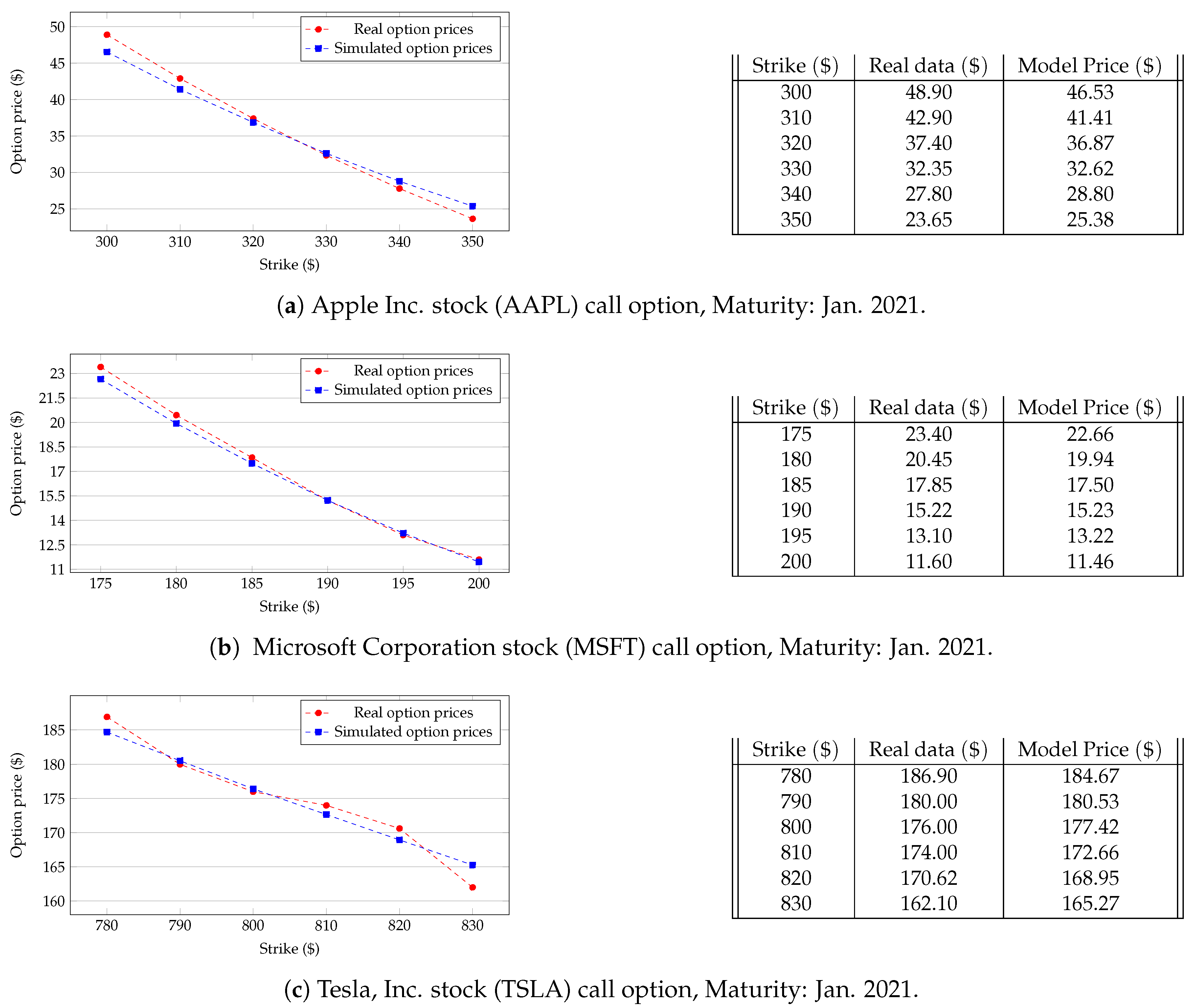
The final step is to empirically apply this method on prices of real-traded options. In particular, we have tested it with derivatives on the same stocks as those considered for the Esscher’s method. In order to estimate the parameters of the historical Lévy process, we used the same time series of log–prices as those of the Esscher’s method (see Section 2.1.2) All the call options under scrutiny expire in January 2021: 11 months from the time of simulation.
In the case of call options on Apple Inc. stock (AAPL) we obtained an average of the absolute values of percentage difference of 3.5794 % : Figure 2a displays the results of such implementation. As regards call options on Microsoft Corporation stock (MSFT), the absolute values of percentage difference is 1.6425 % and the results are shown in Figure 2b. Finally we calibrated our method to the prices of call options on Tesla, Inc. stock (TSLA): Figure 2c shows the outcomes. Here the mean of absolute values of percentage difference settles down at 0.9148 % .
This time we retrieved the real prices from https://finance.yahoo.com, but the same considerations as Remark 3 apply.

4. Conclusions

The main purpose of this research is to quantify the performances of two option pricing methods in a liquid market like NASDAQ. The first approach is based on the Esscher measure, the second one on the calibration to real-traded call option prices with an entropic penalty term.
Our experimental analysis shows that, from a computational point of view, the Esscher method with 10 4 Monte Carlo iterations is far faster than the calibration method: the table in Figure 3 reports the exact execution times that we have obtained with an Asus ZenBook UX31A. This fact is especially noticeable when we need to simulate the prices of options with different maturities and same strike. On the other hand, the calibration method allows generating the entire option chain for a fixed maturity with great precision. Moreover, it is more stable than the previous one, as it provides results closer to real data for a larger range of stock prices.
Comparing averages of absolute values for percentage difference between real and simulated prices, the calibration procedure offers better outcomes than Esscher’s, with the only exception of AAPL call options, where the latter outperforms the former by approximately 42 basis points. Nevertheless, the Esscher method only needs the historical time series of the underlying asset price to be applied, so it is feasible also in markets with few derivatives. This study shows that the Esscher measure is an appealing and efficient solution to price call options in illiquid—or low liquid—financial markets.

5. Future Research

Considering the future work on the subject, one of the directions worth investigating is the Linear Esscher measure method. The importance of focusing on this approach is given by its intrinsic link to the minimal entropy Hellinger martingale measure, as indicated by Rheinländer and Sexton in (Rheinländer and Sexton 2011, Chp. 9), and, in much more detail, by Choulli and Stricker in Choulli and Stricker (2006). Moreover, it would be interesting to extend our study to other asset classes like metal futures, and to compare it with the results obtained in Chen (2011).

Author Contributions

Conceptualization, A.B. and T.R.; methodology, T.R.; software, A.B.; validation, A.B., D.R. and T.R.; formal analysis, A.B., D.R. and T.R.; investigation, A.B., D.R. and T.R.; resources, A.B., D.R. and T.R.; data curation, A.B., D.R.; writing—original draft preparation, A.B., D.R.; writing—review and editing, A.B., D.R. and T.R.; visualization, A.B., D.R.; supervision, T.R.; project administration, T.R.; funding acquisition, T.R. All authors have read and agreed to the published version of the manuscript.

Funding

Open Access Funding by TU Wien. This research received no external funding.

Acknowledgments

We would like to thank Dan Chen for valuable comments. The authors acknowledge TU Wien Bibliothek for financial support through its Open Access Funding Program.

Conflicts of Interest

The authors declare no conflict of interest.

Appendix A. Normal Inverse Gaussian Distribution
In our work, we extensively use the N I G distribution, because it provides a good fit for the analyzed data. A probability measure μ on R is said to be N I G with parameters α , β , μ , δ , where 0 β < α , μ R and δ > 0 , if it has the following density:
f N I G x ; α , β , μ , δ = α π exp δ α 2 β 2 + β x μ K 1 α δ 1 + x μ δ 2 1 + x μ δ 2 ,
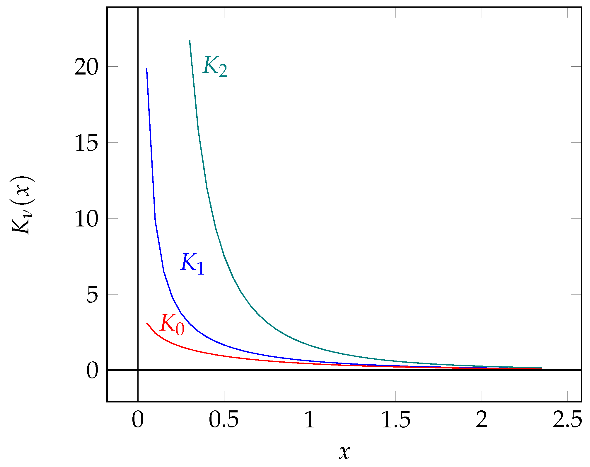
with K 1 that denotes the modified Bessel function of the third kind with index 1 and x R . For a definition of K 1 we refer to Abramowitz and Stegun (1970). The next procedure is the classical construction of such a distribution.
A probability measure μ on R + , B R + is said to be a generalized inverse Gaussian (GIG) distribution with parameters ν R , δ > 0 , γ > 0 if its density with respect to the Lebesgue measure is
f G I G x ; ν , δ , γ = γ δ ν 1 2 K ν γ δ x ν 1 exp 1 2 δ 2 x 1 + γ 2 x , x > 0 .
In order to show that f G I G is a density function, we need the following representation for K ν (Watson 1966, Formula (8), p. 182), the modified Bessel function of the third kind with index ν :
K ν x = 1 2 0 y ν 1 exp x 2 y + 1 y d y , x > 0 .
The computation of the next integral allows us to find the normalization constant in (A2):
0 x ν 1 e 1 2 δ 2 x 1 + γ 2 x d x = 0 x ν 1 e 1 2 γ δ δ γ x 1 + γ δ x d x = δ γ ν 0 y ν 1 e 1 2 γ δ y + 1 y d y = 2 δ γ ν K ν γ δ ,
where in the second equality we made the substitution y = γ δ x . Since K ν > 0 in R + from (A3), we can conclude that f G I G is actually a density function on R + .
Figure A1. K 0 , K 1 , K 2 are the modified Bessel functions of the first three, nonnegative, integer orders, respectively.
Risks 08 00108 g0a1
Let us fix two other parameters α , β R such that 0 β < α . For any μ R , y R + we denote by f N · ; μ , β , y the density of the probability measure on R , B R generated by a random variable X N μ + β y , y . It is possible to introduce a new distribution on R , B R considering the following function:
f G H x ; ν , α , β , μ , δ : = 0 f N x ; μ , β , y f G I G y ; ν , δ , α 2 β 2 d y = 1 2 π α 2 β 2 δ ν 1 2 K ν δ α 2 β 2 0 1 y e 1 2 y x μ β y 2 y ν 1 e 1 2 δ 2 y 1 + α 2 β 2 y d y = 1 2 π α 2 β 2 δ ν 1 2 K ν δ α 2 β 2 e β x μ 0 y ν 1 1 2 exp 1 2 1 y δ 2 + x μ 2 + α 2 y d y = 1 2 π α 2 β 2 δ ν 1 2 K ν δ α 2 β 2 e β x μ δ 2 + x μ 2 α ν 1 2 0 z ν 1 2 1 exp 1 2 z 1 + z α δ 2 + x μ 2 d z = α 2 β 2 ν 2 π δ ν α ν 1 2 K ν δ α 2 β 2 e β x μ K ν 1 2 α δ 2 + x μ 2 δ 2 + x μ 2 1 2 ν , x R ,
where in the last but one equality we made the substitution z = α δ 2 + x μ 2 y and in the last we used (A3).
A straightforward application of Tonelli’s theorem shows that f G H · ; ν , α , β , μ , δ is a density function: the corresponding probability measure on R , B R is called Generalized Hyperbolic distribution.
We recover the N I G density (A1) taking ν = 1 2 in (A4). In fact, for every ν R , it results K ν = K ν and the representation (Abramowitz and Stegun (1970), Formula ( 9.6 . 23 ))
K ν x = π 1 2 x ν Γ ν + 1 2 1 e x t t 2 1 ν 1 2 d t , x > 0 ,
which holds for every ν > 1 2 , enables us to conclude
K 1 2 x = K 1 2 x = π x 2 1 x e x t 1 = π 2 e x x , x > 0 .
As a particular case of Generalized Hyperbolic distribution, the N I G probability measure is infinitely divisible (see, e.g., Barndorff-Nielsen and Halgreen 1977; Eberlein and Hammerstein 2004). The moment generating function for a random variable X N I G α , β , μ , δ is given by
E e z X = exp μ z + δ α 2 β 2 α 2 β + z 2 , α β z α β ,
and its generating triplet (see Appendix B for the definition of this concept) is given by
σ 2 = 0 ν d x = δ α π x e β x K 1 α x d x γ = μ + 2 δ α π 0 1 sinh β x K 1 α x d x .
For an explicit calculation, we refer to the paper Barndorff-Nielsen (1998).

Appendix B. Cumulant Function of Lévy Processes

Fix a probability space Ω , F , P . It is well known that, if X = X t t is a Lévy process, then X t is infinitely divisible for every t R 0 + . On the other hand, for every infinitely divisible probability measure μ on R d , there exists a Lévy process X = X t t , which is unique up to identity in law, such that X 1 μ .
The Lévy–Khintchine representation theorem states that, given an infinitely divisible distribution μ on R d , its characteristic function μ ^ can be written as:
μ ^ z = exp 1 2 z , A z + i γ , z + R d e i z , x 1 i z , x 1 D x ν d x , z R d ,
where D : = x R d : x 1 , γ R d , ν is a measure on R d satisfying
ν 0 = 0 ,     R d x 2 1 ν d x <
and A is a symmetric, positive semidefinite d × d matrix. The representation (A7) of μ ^ by A , ν , γ is unique and the triplet A , ν , γ is called generating triplet of the distribution μ . The generating triplet of a Lévy process X = X t t is the generating triplet of X 1 .
Note that it is not necessary to take 1 D to have integrability in (A7). In fact, let h : R d R d be a bounded function, with h x = x in a neighborhood of 0: we call it a truncation function. Since, for every z R d , in a neighborhood of 0 we have e i z , x 1 i z , h x 1 2 z 2 x 2 and, further, e i z , x 1 i z , h x 2 + C z , x R d , for some positive constant C such that h C in R d , if we put γ h : = γ + R d h x x 1 D x ν d x component wise, then the Lévy–Khintchine formula with respect to h becomes:
μ ^ z = exp 1 2 z , A z + i γ h , z + R d e i z , x 1 i z , h x ν d x , z R d .
We note that only γ h depends on the choice of the truncation function.
It is possible to “extend” the argument of the exponential function in (A7), called characteristic exponent and denoted by ψ , to a subset of C d . Precisely, taking into account the set
C : = c R d : x > 1 e c , x ν d x < ,
we can define the function Ψ : D ˜ C as follows:
Ψ w : = 1 2 w , A w + γ , w + R d e w , x 1 w , x 1 D x ν d x , w D ˜ ,
where D ˜ : = w C d : Re w C . We readily note that i z D ˜ for every z R d and the following equality holds: Ψ i z = ψ z , z R d . In this sense Ψ extends ψ to a subset of C d . We pinpoint that, in this paper, we set u , w : = j = 1 d u j w j , u , w C d , so · , · is not the C d -Hermitian inner product. Theorem 25.17 in Sato (1999) affirms that, if X = X t t is a Lévy process generated by A , ν , γ , then
E e w , X t = e t Ψ w for any w D ˜ , t > 0 :
we call Ψ the cumulant function of X. As we have previously done, we can introduce a truncation function h and express Ψ = Ψ h in D ˜ , where
Ψ h w : = 1 2 w , A w + γ h , w + R d e w , x 1 w , h x ν d x , w D ˜ .
Remark A1.
Let X = X t t be a R d -valued Lévy process defined on a probability space Ω , F , P , Ψ be its cumulant function and θ R d be such that E exp θ , X t < for some t > 0 . By Theorem 25.3 in Sato (1999), this is equivalent to require that θ C . We introduce the random variables
M t : = exp θ , X t t Ψ θ , t 0 .
Note that M = M t t is integrable, by assumption and the fact that t Ψ θ is constant in Ω for every t 0 . Let us construct the minimal augmented filtration F = F t t 0 of X, i.e., F t = σ N F t 0 for any t 0 , where F t 0 t is the natural filtration of the process and N the collection of F -negligible sets; obviously, M is F -adapted. According to (Protter 2005, Chapter I, Theorem 31) F is right-continuous, so it satisfies the usual conditions, as well. If we fix t > s 0 , then using (A9) and the properties of the Lévy-increments we see that M is a martingale with mean 1:
E M t | F s = E e θ , X t t Ψ θ | F s = a . s . e θ , X s s Ψ θ E e θ , X t X s | F s e t s Ψ θ = a . s . M s E e θ , X t s e t s Ψ θ = M s .
Definition A1.
Fix T > 0 and let θ C . The probability measure P θ on F T , with P θ P on F T , defined by d P θ d P : = M T is called the Esscher transform of P with respect to θ. The density process is given by d P θ | F t d P | F t = M t , t 0 , T .

Appendix C. Characteristics of Semimartingales

The aim of this section is to generalize the concept of generating triplet of a Lévy process to semimartingales. Here we mainly follow (Shiryaev and Jacod 2003, Chapter II).
We start off by fixing a stochastic basis ( Ω , F , P ; F ) , with F which satisfies the usual conditions. Given two stopping times S , T , the stochastic interval is the random set
S , T : = t , ω R 0 + × Ω : S ω t T ω ,
and T : = T , T .
Definition A2.
A random set A is called thin if it is of the form A = n T n , where T n n is a sequence of stopping times.
It is important to observe that the sections t R 0 + : t , ω A , for ω Ω , are at most countable when A is a thin set.
Theorem A1.
If X = X t t is a RCLL, adapted process, then the random set Δ X 0 is thin.
We refer to (He et al. 2018, Theorem 3.32) for a proof. Thanks to this result we can easily introduce the next concept.
Definition A3.
Let X = X t t be an adapted, RCLL, R d -valued process. The measure μ X on R 0 + × R d defined by
μ X ω ; d t , d x : = s 1 x 0 Δ X s ω δ s , Δ X s ω d t , d x , ω Ω ,
where δ a ¯ denotes the Dirac measure at a point a ¯ , is called measure associated with its jumps.
We now consider a process X = X t t which is a d-dimensional semimartingale, highlighting that we restrict our attention to RCLL and F -adapted semimartingales. Let h be a truncation function; using the measure μ X it is possible to derive the characteristics of X (see Shiryaev and Jacod 2003, Chp. II, Definition 2.6), which we denote by the triplet B , C , ν X . They are defined up to a P-null set and only B depends on the choice of h.
Every Lévy process—once we endow the probability space in which it is defined with its minimal augmented filtration—is a P I I S process (a RCLL, adapted process which starts at 0 and has independent and stationary increments), which in turn is a semimartingale. Thus, considering a Lévy process L = L t t with generating triplet A , ν , γ h relative to a truncation function h, we can apply (Shiryaev and Jacod 2003, Chp. II, Corollary 4.19) together with the uniqueness of the Lévy–Khintchine representation to express its characteristics as γ h t , A t , d t ν d x .

Appendix D. Laplace Cumulant and Geometric Esscher Measure

On a stochastic basis Ω , F , P ; F , with the filtration F which satisfies the usual conditions of right-continuity and completeness, we define a d–dimensional semimartingale X = X 1 , , X d , i.e., a process which can be decomposed as X = M + A , a sum of a local martingale M and a process A of locally finite variation which is called drift, or additive compensator, of the semimartingale, and with characteristics B , C , ν X relative to a truncation function h (see Appendix B for the definition). In particular, a special semimartingale is a semimartingale where its finite variation part is predictable; such a special semimartingale has a unique semimartingale decomposition. In view of (Shiryaev and Jacod 2003, Chp. II, Proposition 2.9) we can assume, without loss of generality, that ν X t × R d 1 identically. An exposition on semimartingale characteristics is outside of the scope of this paper, for this we refer to Shiryaev and Jacod (2003).
Now we introduce the stochastic logarithm and the stochastic exponential, denoted by L and E , respectively. The symbol · denotes stochastic integration, the exact meaning can vary according to the context. Let X be a semimartingale; the set of stochastic processes which are integrable with respect to X is denoted by L ( X ) . This notion is quite intricate, and it is not the purpose of this article to give an overview on the theory of stochastic integration. For this, we refer to (Protter 2005, Chp. IV, Section 2). The solution of the stochastic integral equation
Y = 1 + Y · X
is denoted as the stochastic exponential E X of the semimartingale X. Here, the process Y = Y t t is defined by Y t : = Y t = lim s t Y s for t > 0 , with Y 0 : = Y 0 . Conversely, if Y is a semimartingale such that both Y and Y do not vanish, then the process
X = 1 Y _ · Y ,
denoted by L ( Y ) , is called the stochastic logarithm of Y, and is the unique semimartingale such that
Y = Y 0 E X .
For a detailed exposition of these concepts we refer to (Shiryaev and Jacod 2003, Chp. II, Section 8).
Definition A4.
Let θ L X be an admissible strategy such that θ · X is exponentially special, i.e., exp ( X ) is a special semimartingale. The Laplace cumulant K ˜ X θ of X at θ is the additive compensator of the real-valued, special semimartingale
L exp θ · X .
The modified Laplace cumulant K X θ of X at θ is the process
K X θ : = log E K ˜ X θ .
Note that the additive compensator of the process
L exp θ · X = 1 exp θ · X · exp θ · X
is predictable because exp θ · X is special and 1 exp θ · X is predictable. Therefore, L exp θ · X is a special semimartingale and the definition of K ˜ X θ is well posed. As far as K X θ is concerned, recalling (Shiryaev and Jacod 2003, Chp. III, Theorem 7.4) we have
Δ K ˜ X θ t = R d e θ t , x 1 ν X { t } × d x > 1 , t 0 .
Thus, the stochastic exponential in (A10) is strictly positive and the process K X θ is well defined, as well.
If θ · X is exponentially special, then K X θ is its exponential compensator, see (Shiryaev and Jacod 2003, Chp. III, Theorem 7.14). This means that the process Z θ = Z t θ t , defined by Z t θ : = exp θ · X t K X ( θ ) t , t 0 , is a local martingale starting at Z 0 θ = 1 . We now recall the concept of uniform integrability.
Definition A5.
A non-empty set Φ of real-valued random variable defined on a probability space Ω , F , P is uniformly integrable if
lim n sup X Φ E X 1 X n = 0 .
Supposing that Z θ is a uniformly integrable martingale, then we can set P θ ( d ω ) : = Z θ P ( d ω ) , where Z t Z a.s. and in L 1 as t . It is straightforward to show that Z θ is the density of P θ relative to P; besides, these two distributions are locally equivalent as Z t θ > 0 , t 0 .
The following result (Shiryaev and Jacod 2003, Chp. III, Theorem 7.18) establishes a necessary and sufficient condition such that the process S i : = S 0 i exp X i , S 0 i R + is a P θ -local martingale for every i = 1 , , d .
Theorem A2.
Let θ L X be such that θ · X is exponentially special and Z θ is a uniformly integrable martingale. Define
θ j ( i ) : = θ j , j i θ i + 1 , j = i .
Then the processes S i = S 0 i exp X i are P θ -local martingales if and only if θ ( i ) · X is exponentially special and K X θ ( i ) = K X θ up to evanescence for every i = 1 , , d .
We call P θ geometric Esscher measure, or Esscher martingale transform for exponential processes. For d = 1 , in case the geometric Esscher measure exists, (Kallsen and Shiryaev 2002, Theorem 4.2) provides its uniqueness: this means that, if we find another process θ ˜ L X such that S = S 0 exp X is a P θ ˜ -local martingale, then P θ ˜ = P θ .
We conclude with some technical results. Let θ L X be such that θ · X is exponentially special. By (Shiryaev and Jacod 2003, Chp. III, Theorem 7.4) and (Shiryaev and Jacod 2003, Chp. II, Proposition 2.9) we can write K ˜ X θ = κ ˜ θ · A , where
κ ˜ θ t : = θ t , b t + 1 2 θ t , c t θ t + R d e θ t , x 1 θ t , h x F t ( d x ) , t 0 .
The next lemma (Kallsen and Shiryaev 2002, Lemma 2.11) allows us to express the drift process as a function of the characteristics of the semimartingale.
Lemma A1.
Let θ L X be such that θ · X is a special semimartingale. Then its drift process D X θ = δ θ · A , where
δ θ t : = θ t , b t + R d θ t , x h x F t ( d x ) , t 0 .
Finally, we use Girsanov’s theorem to compute the characteristics B θ , C θ , ν X θ of X under P θ —provided its existence—relative to the same h:
B θ i = B i + c i · θ · A + h i ( x ) e θ t , x 1 + W ^ θ t 1 🟉 ν X , i = 1 , , d C θ = C ν X θ d t , d x = e θ t , x 1 + W ^ θ t ν X d t , d x ,
where W ^ θ t : = R d e θ t , x 1 ν X t × d x , t 0 . Note that W ^ θ t = Δ K ˜ X θ t > 1 , t 0 .
Remark A2.
For ω Ω , t 0 and G B R d , we have:
ν X ω ; t × G = R 0 + d A s ω R d 1 t × G s , x F s , ω d x = t d A s ω R d 1 G x F t , ω d x = F t , ω G t d A s ω .
Moreover, as t d A s ω = A t ω A t ω , if the function A · ω is continuous in t, then ν X ω ; t × d x is the null measure on B R d , which implies that W ^ θ t ω = 0 .

Appendix E. Lévy Processes on Skorohod Space and Relative Entropy of Distributions

Let Ω , F , P be a probability space which carries a R d -valued, additive process X t t with system of generating triplets A t , ν t , γ t t . For every t 0 we define x t : D R d , where D is the Skorohod Space, as x t ξ : = ξ t , ξ D , and we introduce the σ -algebra F D : = σ x t , t 0 . Now we are in the position to define a natural filtration F : = F t t 0 on the measurable space D , F D , where F t : = σ x s , 0 s t , t 0 . Since X t t is an RCLL process, we set the map ϕ : Ω D as ϕ ω : = X · ω , ω Ω , where X · ω : 0 , R d , with X · ω t : = X t ω for any t 0 . The function ϕ is F / F D measurable, since
F D = σ x t , t 0 = σ x t 1 B , B B R d , t 0
and, for every B B R d and t 0 , we have
ϕ 1 x t 1 B = ω Ω : ϕ ω x t 1 B = ω Ω : X · ω x t 1 B = ω Ω : X t ω B = X t 1 B F .
This enables us to construct the pushforward measure P D on D , F D , that is,
P D A : = P ϕ 1 A = P ϕ 1 A , A F D .
We now focus on the stochastic process x t t defined on the probability space D , F D , P D . Fix a cylinder set C F D , i.e.,
C = ξ D : ξ t 1 B 1 , , ξ t n B n ,
for some t 1 < t 2 < < t n , B 1 , , B n B R d and n N . By (A13), we have
P D x t 1 B 1 , , x t n B n = P D C = P ϕ 1 C = P X t 1 B 1 , , X t n B n .
Thus, x t t and X t t are identical in law, whence x t t is an additive process with the same system of generating triplets as X t t . Specifically, if X t t were a Lévy process, then x t t would inherit the temporal homogeneity, so it would be a Lévy process, as well.
Consider two Lévy processes x t t , P and x t t , P on the Skorohod space D , F D endowed with the filtration F . The next theorem (Sato 1999, Theorems 33.1 & 33.2) provides us with conditions which ensure P | F t P | F t for any t > 0 .
Theorem A3.
Let x t t , P , x t t , P be Lévy processes on R d with generating triplets A , ν , γ and A , ν , γ , respectively. Then the following properties are equivalent:
(a) 
P | F t P | F t for every t > 0 ;
(b) 
the generating triplets satisfy: A = A , ν ν .
Besides, considering the function ϕ : R d R defined by ϕ : = log d ν d ν ,
R d e ϕ x / 2 1 2 ν d x < , γ γ x 1 x ν ν d x A y , y R d .
In this case, chosen η R d such that γ γ x 1 x ν ν d x = A η , there exists a process U = U t t defined on D which satisfies the following properties:
(i) 
U is a P-Lévy process on R with generating triplet
σ U 2 = η , A η ν U = ν ϕ 1 | R \ 0 γ U = 1 2 η , A η R e y 1 y 1 D y ν ϕ 1 d y ;
(ii) 
E P e U t = E P e U t = 1 for every t 0 ;
(iii) 
e U t = d P | F t d P | F t P a . s . for every t > 0 .
An explicit expression of the process U, which is unique up to identity in law, can be retrieved in (Sato 1999, Theorem 33.2).
Definition A6.
Given two probability measures P , P on a measurable space Ω , F , the relative entropy H P , P of P with respect to P is defined by
H P , P : = Ω log d P d P ω P d ω , if P P , otherwise .
Recall that given two distributions P , P on Ω , F we have H P , P 0 , with equality if and only if P = P .
We finally present a theorem which explicitly computes the relative entropy of two equivalent Lévy processes in the Skorohod space as a function of their generating triplets.
Theorem A4.
Let x t t , P , x t t , P be Lévy processes on R d defined on D , F D with generating triplets A , ν , γ and A , ν , γ , respectively. Suppose that P | F t P | F t for every t > 0 and choose η R d such that
γ γ x 1 x ν ν d x = A η .
Assume also that E P g U t < for some t > 0 , where g x : = x 1 e x , x R . Then for every T > 0 it results
H P | F T , P | F T = T 2 η , A η + T R d d ν d ν log d ν d ν + 1 d ν d ν d ν .
Proof. 
Let us fix a finite time horizon T > 0 . For any z 0 , 1 , by assumption we have
E P e z U T = R e z x P U T d x R g x P U T d x < .
We introduce the moment generating function M U T z : = E P e z U T = e T Ψ z , z 0 , 1 , where Ψ is the cumulant function of the Lévy process U, i.e.,
Ψ z = 1 2 σ U 2 z 2 + γ U z + R e z x 1 z x 1 D x ν U d x , z 0 , 1 ,
and the last equality is ensured by (A9) in Appendix B. Actually M U T is well defined for z = 1 too, with M U T 1 = E P e U T = e T Ψ 1 = 1 , by A3 in Theorem A3. We can see that M U T is differentiable in 0 , 1 with M U T · = E P U T e · U T . Indeed, for every z 0 , 1 , M U T z = R e z x P U T d x and we can derive under integral sign since
x e z x g x L 1 P U T , z 0 , 1 , x R .
At this point the dominated convergence theorem readily shows that
lim z 1 M U T z = R x e x P U T d x = E P U T e U T .
On the other hand, we introduce the function f z : = e T Ψ z , z 0 , 1 .
Even in this case we can affirm that f is differentiable in its domain, with derivative provided by f = T e T Ψ Ψ . In particular the following equality is true:
Ψ z = σ U 2 z + γ U + R x e z x x 1 D x ν U d x , z 0 , 1 .
In fact, we can derive under the integral sign in (A15) as, for every z 0 , 1 , it results that x e z x x 1 + e , x D , with x e z x x C x 2 in a neighborhood of 0 for some constant C > 0 which is independent of z. Moreover, x e z x g x for x > 1 , with x > 1 x e x ν U d x < by Theorem 25.3 in Sato (1999). Applying another time the Lebesgue’s convergence theorem we arrive at
lim z 1 M U T z = T e T Ψ 1 σ U 2 + γ U + R x e x x 1 D x ν U d x .
Therefore
E P U T e U T = T e T Ψ 1 σ U 2 + γ U + R x e x x 1 D x ν U d x = T 2 η , A η + T R d d ν d ν log d ν d ν + 1 d ν d ν d ν ,
using the expression of σ U 2 , ν U , γ U in A3 of Theorem A3. Since d P | F t d P | F t = e U t for every t > 0 (see A3 in Theorem A3) and
H P | F T , P | F T = D d P | F T d P | F T log d P | F T d P | F T d P = E P U T e U T ,
we obtain (A14) and complete the proof. □
Remark A3.
In the case of two R -valued Lévy processes x t t , P , x t t , P with generating triplets σ 2 , ν , γ and σ 2 , ν , γ , respectively, under the hypothesis of the previous theorem (A14) reduces to
H P | F T , P | F T = T 2 σ 2 η 2 + T R d ν d ν log d ν d ν + 1 d ν d ν d ν .
If we are dealing with pure jump processes (e.g., N I G processes), the first term in the sum of the right-hand side is 0; if instead σ 2 > 0 , then we have
T 2 σ 2 η 2 = T 2 σ 2 γ γ x 1 x ν ν d x 2 ,

References

  1. Abramowitz, Milton, and Irene A. Stegun. 1970. Handbook of Mathematical Functions: With Formulas, Graphs, and Mathematical Tables. Washington, DC: US Government Printing Office, vol. 55. [Google Scholar]
  2. Asmussen, Søren, and Jan Rosiński. 2001. Approximations of Small Jumps of Lévy Processes with a View towards Simulation. Journal of Applied Probability 38: 482–93. [Google Scholar] [CrossRef]
  3. Barndorff-Nielsen, Ole E. 1998. Processes of Normal Inverse Gaussian Type. Finance and Stochastics 2: 41–68. [Google Scholar] [CrossRef]
  4. Barndorff-Nielsen, Ole, and Christian Halgreen. 1977. Infinite Divisibility of the Hyperbolic and Generalized Inverse Gaussian Distributions. Probability Theory and Related Fields 38: 309–12. [Google Scholar] [CrossRef]
  5. Benth, Fred Espen, and Maren Diane Schmeck. 2014. Pricing futures and options in electricity markets. In The Interrelationship Between Financial and Energy Markets. Berlin/Heidelberg: Springer, pp. 233–60. [Google Scholar]
  6. Benth, Fred Espen, Jurate Saltyte Benth, and Steen Koekebakker. 2008. Stochastic Modelling of Electricity and Related Markets. Singapore: World Scientific, vol. 11. [Google Scholar]
  7. Carr, Peter, and Dilip Madan. 1999. Option Valuation using the Fast Fourier Transform. Journal of Computational Finance 2: 61–73. [Google Scholar] [CrossRef] [Green Version]
  8. Chen, Dan. 2011. Three Essays on Pricing and Hedging in Incomplete Markets. Ph.D. thesis, The London School of Economics and Political Science (LSE), London. [Google Scholar]
  9. Choulli, Tahir, and Christophe Stricker. 2006. More on minimal entropy–Hellinger martingale measure. Mathematical Finance 16: 1–19. [Google Scholar] [CrossRef]
  10. Cont, Rama, and Peter Tankov. 2004a. Financial Modelling with Jump Processes. Boca Raton: Chapman and Hall/CRC. [Google Scholar]
  11. Cont, Rama, and Peter Tankov. 2004b. Nonparametric calibration of jump-diffusion option pricing models. Journal of Computational Finance, Incisive Media 7: 1–49. [Google Scholar] [CrossRef] [Green Version]
  12. Eberlein, Ernst, and Ernst August V. Hammerstein. 2004. Generalized hyperbolic and inverse Gaussian distributions: Limiting cases and approximation of processes. In Seminar on Stochastic Analysis, Random Fields and Applications IV. Berlin: Springer, pp. 221–64. [Google Scholar]
  13. Esscher, F. 1932. On the Probability Function in the Collective Theory of Risk. Skandinavisk Aktuarietidskrift 15: 175–95. [Google Scholar]
  14. Gerber, Hans U., and Elias SW Shiu. 1994. Option Pricing by Esscher Transforms. Transactions of the Society of Actuaries 46: 99–191. [Google Scholar]
  15. Hell, Philipp, Thilo Meyer-Brandis, and Thorsten Rheinländer. 2012. Consistent factor models for temperature markets. International Journal of Theoretical and Applied Finance 15: 1250027. [Google Scholar] [CrossRef]
  16. He, Sheng-wu, Jia-gang Wang, and Jia-an Yan. 2018. Semimartingale Theory and Stochastic Calculus. New York: Routledge. [Google Scholar]
  17. Iacus, Stefano Maria. 2011. Option Pricing and Estimation of Financial Models with R. New York: John Wiley and Sons. [Google Scholar]
  18. Jeanblanc, Monique, Marc Yor, and Marc Chesney. 2009. Mathematical Methods for Financial Markets. Berlin: Springer. [Google Scholar]
  19. Kallsen, Jan, and Albert N. Shiryaev. 2002. The Cumulant Process and Esscher’s Change of Measure. Finance and Stochastics 6: 397–428. [Google Scholar] [CrossRef] [Green Version]
  20. Klüppelberg, Claudia, Alexander Lindner, and Ross Maller. 2004. A Continuous Time GARCH Process Driven by a Lévy Process: Stationarity and Second Order Behaviour. Journal of Applied Probability 41: 601–622. [Google Scholar] [CrossRef] [Green Version]
  21. Lee, Young, and Thorsten Rheinländer. 2012. Optimal martingale measures for defaultable assets. Stochastic Processes and their Applications 122: 2870–84. [Google Scholar] [CrossRef] [Green Version]
  22. Lewis, PA W., and Gerald S. Shedler. 1979. Simulation of Nonhomogeneous Poisson Processes by Thinning. Naval Research Logistics Quarterly 26: 403–13. [Google Scholar] [CrossRef]
  23. Morozov, Vladimir Alekseevich. 1966. On the solution of functional equations by the method of regularization. Doklady Akademii Nauk 167: 510–12. [Google Scholar]
  24. Protter, P. E. 2005. Stochastic Integration and Differential Equations, 2nd ed. Stochastic Modelling and Applied Probability. Berlin: Springer, vol. 21. [Google Scholar]
  25. Rheinländer, Thorsten, and Jenny Sexton. 2011. Hedging Derivatives. Singapore: World Scientific, vol. 15. [Google Scholar]
  26. Rudin, Walter. 1987. Real and Complex Analysis, 3rd ed. Mathematics Series; New York: McGraw-Hill Higher Education. [Google Scholar]
  27. Sato, Ken-Iti. 1999. Lévy Processes and Infinitely Divisible Distributions. Cambridge: Cambridge University Press. [Google Scholar]
  28. Shiryaev, Albert, and Jean J. Jacod. 2003. Limit Theorems for Stochastic Processes. A Series of Comprehensive Studies in Mathematics; Berlin: Germany, vol. 288. [Google Scholar]
  29. Shreve, Steven E. 2004. Stochastic Calculus for Finance II (Continuous–Time Models). Springer Finance Textbooks. Berlin: Springer, vol. 11. [Google Scholar]
  30. Van Heerwaarden, Angela E., Rob Kaas, and Marc J. Goovaerts. 1989. Properties of the Esscher premium calculation principle. Insurance Mathematics and Economics 8.4 335: 261–67. [Google Scholar] [CrossRef]
  31. Watson, George Neville. 1966. A Treatise on the Theory of Bessel Functions, 2nd ed. Cambridge: Cambridge University Press. [Google Scholar]
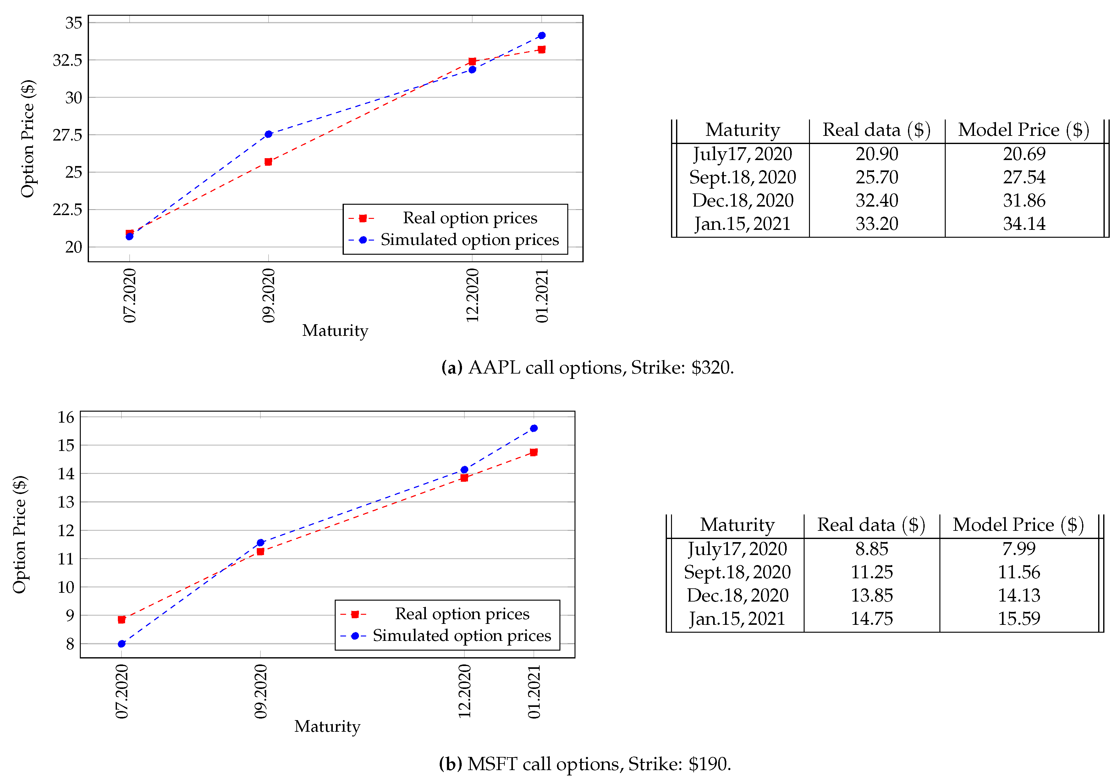
Figure 1. Numerical experiments for the Esscher method.
Risks 08 00108 g001aRisks 08 00108 g001b
Figure 2. Numerical experiments for the calibration method.
Risks 08 00108 g002
Figure 3. Computational times (in seconds) of both methods (with an Asus ZenBook UX31A).
Risks 08 00108 g003
Publisher’s Note: MDPI stays neutral with regard to jurisdictional claims in published maps and institutional affiliations.