Article

Loss Reserving Estimation With Correlated Run-Off Triangles in a Quantile Longitudinal Model

by
Ioannis Badounas
and
Georgios Pitselis
*
Department of Statistics and Insurance Science, University of Piraeus, 18534 Piraeus, Greece
*
Author to whom correspondence should be addressed.
Risks 2020, 8(1), 14; https://doi.org/10.3390/risks8010014
Submission received: 31 July 2019 / Revised: 28 December 2019 / Accepted: 9 January 2020 / Published: 3 February 2020
(This article belongs to the Special Issue Loss Models: From Theory to Applications)

Abstract

:
In this paper, we consider a loss reserving model for a general insurance portfolio consisting of a number of correlated run-off triangles that can be embedded within the quantile regression model for longitudinal data. The model proposes a combination of the between- and within-subportfolios (run-off triangles) estimating functions for regression parameter estimation, which take into account the correlation and variation of the run-off triangles. The proposed method is robust to the error correlation structure, improves the efficiency of parameter estimators, and is useful for the estimation of the reserve risk margin and value at risk (VaR) in actuarial and finance applications.

1. Introduction

The protection of the policyholders and the financial stability of the insurance market industry is a crucial aspect and regulatory authorities intervene to ensure it. Based on Solvency II and IFRS Phase II regulations, each insurance or reinsurance company is obliged to evaluate its insurance liabilities on a risk-adjusted basis to allow for uncertainty in cash flows that arises from the liability of the insurance contracts. Australian Prudential Regulation Authority (APRA) requires estimating a 75th percentile of the distribution of outstanding claims for recording in profit and loss statements and the risk margin should be established on a basis that is intended to secure the insurance liabilities of the insurance company at a given level of sufficiency ( 75 % ).
In recent years, quantile regression has become a very popular methodology that has incorporated several new reforms in insurance and finance. The least squares estimators investigate only changes in the mean when the entire shape of the claims distribution may change dramatically. Quantile regression characterizes any particular point of a distribution and thus provides a more complete description of the distribution in comparison to linear regression. Quantile regression techniques can differentiate risk factors that lead to high level claims from those that lead to low level claims. Quantile regression estimation may be more efficient than the ordinary least squares when the distribution is not normal. Furthermore, quantile regression is more robust against outliers and does not require the specification of any error distribution. Therefore, quantile regression may be more appropriate than least squares estimation in the context of the insurance industry (see Buchinsky 1998; Koenker 2005).
In the actuarial literature, few papers deal with quantiles. Pitt (2006) used censored regression quantiles to analyze claim termination rates at different quantiles of the distribution of claim duration for income protection insurance. Chan et al. (2008) proposed a robust Bayesian analysis of loss reserves data using the generalized t -distribution. Dong et al. (2015) presented in detail the use of parametric and nonparametric quantile regression in non-life applications. Nevertheless, the above approaches have been used for univariate quantile regression models and are suitable for a single line of business (single run-off triangle).
In this paper, we consider a quantile regression application in a multivariate context alternative to a multivariate Chain Ladder model for a portfolio of within and between correlated run-off triangles. For a dependent line of business, it is difficult to describe and specify the underlying correlation structure, which may prevent insurance practitioners from using the quantile regression. We propose a reserving problem for a non-life insurance portfolio consisting of several run-off subportfolios corresponding to different lines of business that can be embedded within the quantile regression longitudinal model and can provide solutions to the estimation of more extreme V a R s and capital margins.
The remainder of this paper is structured as follows. Section 2 presents the types of dependence (correlation) modeling in loss reserving triangles. In Section 3, we present brief introductions of quantile functions and quantile regression. Section 4 illustrates how correlated run-off triangles can be embedded in a quantile regression longitudinal model. In Section 5, we present a numerical implementation of the longitudinal quantile regression model with two run-off triangles. Section 6 provides the calculation of the risk margin (RM) based on the solvency capital requirement (SCR) estimation and according to the cost-of-capital (CoC) methodology. Finally, in Section 7, some concluding remarks are presented.

2. Dependence (Correlation) Modeling in Loss Run-Off Triangles

In this section, we highlight three types of dependence structures that may appear in loss reserving estimation. In many stochastic claims reserving models, in a single line of business, it is assumed that accident years are independent. In practice, it is evident that different accident years are not independent because of accounting year effects, claims inflation, and other exogenous factors that affect all accident years simultaneously. As pointed out by Ajne (1994) and many other researchers, when dealing with a portfolio with several lines of business, the Chain Ladder predictors for the whole portfolio differ from the sums of the Chain Ladder predictors for the different individual lines of business, because the dependence structure between the subportfolios of a portfolio is not taken into consideration. Dependence modeling was also discussed by Merz et al. (2012).

2.1. Correlation Within Claims Reserving Triangles

Barnett and Zehnwirth (2000) studied calendar year effects within probabilistic trend family models, which allowed calculating distributions of, and correlations between, future payment streams. De Jong (2012), based on time series models, investigated the correlation between accident and calendar years within triangles. In this spirit, Wuthrich (2010) presented a Bayesian inference approach that allows for the study of accounting (calendar) year effects. By restricting to the lognormal approach to chain-ladder-type models, Kuang et al. (2011) proposed a method suitable for cases where there is a sudden change in the economic environment affecting the policies for all accident years in the reserving triangle. Pešta and Okhrin (2014) proposed a generalized time series model that allows for modeling the conditional mean and variance of the claim amounts, for the claims development. They used a copula framework to incorporate modeling dependencies within the loss triangles.

2.2. Correlation Between Claims Reserving Triangles

The dependence structure between lines of business (run-off triangles) that is related to the accurate estimation of risk’s diversification is very important to the solvency capital requirement (SCR) the company should hold in order to remain healthy and avoid holding unnecessarily high levels of capital (see Avanzi et al. (2016b)).
Clark (2006), by using a times series model, estimated the correlation between future payments, due to inflation, in two or more loss reserving run-off triangles, concluding that the payments move with inflation and the variability due to inflation can be related to economic forecast models. When companies have several lines of business, it is useful to examine the presence of possible dependencies within the structure of the company and investigate the financial effect of these dependencies. Barnett and Zehnwirth (2000) proposed a model that allows dependency between all the observations that belong to the same calendar year for each line of business. According to Braun (2004), the correlation between run-off triangles can be attributed to the claims inflation affecting all or most of the run-offs of a portfolio in a similar way. Shi and Frees (2011) used copulas to model the association among multiple run-off triangles and Abdallah et al. (2015) assumed a dependence structure that links the calendar years of different lines of business. Zehnwirth and Barnett (2001) considered a more complicated situation of n correlated loss triangles. Braun (2004) extended the distribution-free method of Mack (1993) to estimate the prediction error of the Chain Ladder method for a portfolio of several correlated run-off triangles. Pröhl and Schmidt (2005) proposed a multivariate Chain Ladder method that is suitable for a portfolio consisting of several subportfolios with a certain dependence structure.
By using the theory of linear mixed models, Antonio and Beirlant (2006) built a flexible loss reserving model in the framework of longitudinal data. Quarg and Mack (2004) proposed a bivariate Chain Ladder predictor for the paid and incurred aggregate claims of the same portfolio aiming to reduce the gap between the univariate Chain Ladder predictors for the paid and incurred aggregate claims of the same portfolio. Taylor and Mcguire (2005, 2007) considered the claims reserving problem in a multivariate context and generalized linear models were used to estimate loss reserves of several stochastically dependent lines of business, individually and in aggregate. Schmidt (2006) provided a review on recent multivariate models and methods of loss reserving. Merz and Wüthrich (2008a, 2008b) considered the multivariate Chain Ladder method for a portfolio of N correlated run-off triangles based on multivariate age-to-age factors and derived an estimator for the mean square error of prediction for the Chain Ladder predictor of the ultimate claim of the total portfolio. Shi and Frees (2011) demonstrated the role of dependencies in the aggregation of claims from multiple run-off triangles, proposing a copula regression model for the prediction of unpaid losses for dependent lines of business. Zhang (2010) presented a general multivariate stochastic reserving model by using the seemingly unrelated regression technique. This model not only specifies contemporaneous correlation, but also allows structural connections among triangles. Hudecová and Pešta (2013) proposed the application of generalized estimating equations (GEE) for the estimation of claims reserves, where claim triangles are handled as panel data, assuming dependent claim amounts within the same accident year. De Jong (2012) developed and applied a model for loss triangles that facilitates the structuring and measurement of dependence between loss triangles. Bermudez et al. (2013), by using linear regression techniques and copulas, and assuming several dependence structures between lines of business, estimated the risk-based capital reserve for the economic capital requirements under the Standard Model and the Internal Model approach. Their sensitivity analysis on the correlation matrix assumptions between lines of business showed that modifications of the correlation and dependence assumptions have a significant impact on the solvency capital requirement (SCR) estimation, under Solvency II regulations. In insurance applications, normality assumptions may be misleading as a measure of dependency in the tails of the variables. The impact of loss triangle dependence on risk margins was also considered by Hubert et al. (2017), who proposed the FastSUR algorithm, in order to robustify the general multivariate Chain Ladder method of Zhang (2010), where the parameters were estimated using seemingly unrelated regression(SUR). Based on MM-estimators, Peremans et al. (2018) proposed a robust alternative that estimates the SUR parameters in a more outlier resistant way.
Avanzi et al. (2016a, 2016b) proposed a multivariate Tweedie approach to capture cell-wise dependence and the dependency between business segments in the non-life insurance industry, respectively, in loss reserving. In addition, Avanzi et al. (2018) constructed a broad and flexible family of models, where dependency is induced by common shock components. For an extensive analysis of loss reserving techniques, the reader may refer to the books of Taylor (2000), Wuthrich and Merz (2008) and Radtke et al. (2012).

2.3. Correlation Within and Between Claims Reserving Triangles

In actuarial applications, an insurance portfolio is subdivided into several homogeneous lines of business (subportfolios). Losses from a line of business can be viewed as a financial risk. Social and economic environment may affect several lines of business of an insurance portfolio, simultaneously. Thus, we may consider that, in addition to within correlation, insurance lines of business (run-off triangles) are related to each other due to the calendar effects. Zhang et al. (2012) proposed a Bayesian non-linear hierarchical model, where data from individual companies are treated as repeated measurements of various run-off triangles of claims, thus respecting the correlation between successive observations. Shi et al. (2012) examined calendar year effects in a multivariate loss-reserving context through a log-normal model. They used random effects to accommodate the correlation due to accounting year effects within and between run-off triangles. This specification is in line with De Jong (2012), who introduced the calendar year effects through the correlation matrix. In the spirit of Shi et al. (2012), Merz and Wüthrich (2008a) defined a multivariate log-normal model that allows modeling both dependence between different run-off triangles and dependence within run-off triangles, such as claims inflation.

2.4. Why Quantile Regression Models with Correlated Run-off Triangles?

In the insurance practice, some regulation rules indicate that some changes over time occurred across the claim distribution. Therefore, it is very important to investigate these changes at different points of the distributions. For example, Australian insurance regulations require that a risk margin should be established at 75% percentile of the discounted value less than the best estimate (see Pitt (2006)). Most studies consider only correlation as a measure of dependency, focusing on reserving at mid-range V a R s . Consideration of capital margins at more extreme V a R s opens up the question of tail dependency, and a whole new field of exploration (see Avanzi et al. (2016b)).
Each quantile regression characterizes a particular point of a distribution, and thus provides more complete description of the distribution, taking into account the correlations in the tail of distributions. Furthermore, quantile regression is more robust against outliers and does not require specifying any error distribution (see Fu and Wang (2012)).
One implication of our model is the diversification effect of a portfolio of reserve risks and can be used as a risk measure with applications in actuarial science. Practically, our quantile approach leads to a provision of a specified probability, say 80%, sufficient to cover the run-off claims. Adding the necessary margin to the central estimate, the evaluation of the claims liability is provided and the provision is sufficient to cover the future liabilities.

3. Preliminaries on Quantile Functions and on Quantile Regression

Here, we provide some preliminaries on quantile regression that are needed below for loss reserving estimation.

3.1. Quantile Function

For a random variable Y with cumulative distribution function F Y ( y ) = P ( Y y ) , the θ th quantile of Y is defined as the inverse function
Q Y ( θ ) = F Y 1 ( θ ) = inf { y : F ( y ) θ } ,
where 0 θ 1 . In case that F ( · ) is a strictly increasing and continuous probability distribution function, F Y 1 ( θ ) is the unique real number t such that F ( t ) = θ (Gilchrist 2000).
Quantiles are connected with operations of ordering the sample observations that are used to define them. For a random sample { y 1 , , y n } of Y , the general θ th sample quantile ξ ( θ ) may be formulated as the solution of the optimization problem
min ξ i = 1 n ρ θ ( y i ξ ) , w h e r e ρ θ ( z ) = z ( θ I ( z < 0 ) )
and I ( · ) denotes the indicator function. This loss function is an asymmetric absolute loss function because it is a weighted sum of absolute deviations, where the weight ( 1 θ ) is assigned to the negative deviations while the weight θ is assigned to the positive deviations.

3.2. Quantile Regression Estimation

In the regression case, we assume a sample ( Y i , x i ) , i = 1 , . . . , n , where Y i is the dependent variable, x i is a k × 1 vector of explanatory variables, and β is a k × 1 vector of coefficients. The general linear model has the form
Y i = x i T β + u i , a n d E ( Y i | x i ) = x i T β ,
while the θ th conditional quantile of Y i given x i can be written as (see Koenker and Basset 1982)
Q Y i ( θ | x i ) = x i T β θ .
We consider the θ th sample quantile q ^ i ( θ ) . Mosteller proved the limiting normality of ξ ^ Y i | x i θ that provides a realization of the least estimation of the form
q ^ i θ = x i T β θ + u i ,
where β ( θ ) is a vector to be estimated and u i is the error term. The linear conditional quantile function, Q ( θ | X = x ) = x β ( θ ) , can be estimated by solving
min β 1 n i = 1 n ρ θ ( u i ) = min ( β ) i : y i x i β θ | Y i x i T β | + i : Y i < x i T β ( 1 θ ) | Y i x i T β | ,
where ρ θ ( t ) is already defined in Equation (2) and I ( · ) is the indicator function for any quantile θ ( 0 , 1 ) . The case θ = 1 / 2 , which minimizes the sum of absolute residuals, corresponds to median regression, which is also known as L 1 regression. The minimization of Equation (6) was produced by Koenker and D’Orey (1994).
Under certain conditions, for independent observations, the asymptotic variances for u i can be obtained as (see Buchinsky 1998)
w θ = θ ( 1 θ ) n f 2 ( F 1 ( θ ) )
and the covariance matrix of β ^ θ is
Σ ^ θ = ( X T Ω θ 1 X ) 1 , w i t h Ω θ = w θ . I n × n .
With quantile regression, we can show how various financial characteristics are different at different quantiles. Thus, the quantile regression method allows the marginal effects to change for claims at different points in the conditional distribution by estimating β p using several different values of p , p ( 0 , 1 ) . This means that the quantile regression allows for parameter heterogeneity across different types of claims.

4. Correlated Run-Off Triangles in a Quantile Longitudinal Model

The reserving procedure for multiple run-off triangles is an important issue of an insurance company because the connections among the triangles may show correlations which are initially unknown. The correlations of different lines of business may produce more efficient estimations for the total reserve. If for example the two run-off triangles are positively correlated, then the variability of the total reserves exceeds the sum of variabilities of the total reserve from each triangle. Ajne (1994) noted the commonly used approach in actuarial practice, which is the division of the portfolio into several subportfolios and then making calculations using each single line of business. However, this method ignores the dependencies among the subportfolios.
When the run-off triangles are linked with a known structure, such as the paid and incurred triangles, then the Munich Chain Ladder (MuCL) model by Quarg and Mack (2004) is a good method of estimation. Moreover, instead of studying the structural correlations, the correlations between the triangles is an important issue and several papers have been produced (e.g., Braun (2004); Kremer (2005); Schmidt (2006); Merz and Wüthrich (2008a, 2008b)). According to Holmberg (1994), correlations in a run-off triangle may arise among losses as they develop over time or in different accident years. Other authors have studied correlations over calendar year incorporating the trends of inflation which appear. Harrison and Hulin (1989) used generalized estimating equations (GEE) as a promised analytic tool that takes into consideration the correlation of responses within a specific subject for response variables. A more interesting characteristic of these equations is the flexibility they have to analyze not normally distributed response variables.
Suppose that N run-off triangles are available and i { 1 , 2 , , N } refers to the i th triangle while r { 1 , 2 , , I } refers to the accident year and j { 1 , 2 , , I } refers to the development year. Denote Y r j = ( Y r j ( 1 ) , , Y r j ( N ) ) T the n N × 1 vector with the incremental losses at accident year r and development year j for all triangles N .
Denote D = { Y r j , r + j I + 1 , 1 r I , 1 j I } as the observed losses, D · , j = { Y r j , 1 r I , j k } as the losses up to development year k (including it), and D r , j = { Y r j , k j } as the losses for accident year r up to development year j (including it). According to the data, the sets D · , j and D r , j are the observed values and should be used to estimate the adequate reserve to fund losses that have been incurred but not yet developed.
Here, we are not going to use a triangulation form to model the data. Let y i k be the k th measurement for the i th subject (triangle), which describes the total claims amount or the number of claims at the i run-off triangle for i = 1 , , N , k = 1 , , n i where n i is the number of the observed data of the triangle i . We consider the case where longitudinal data analyses are based on a linear regression model such as
y i k = x i k T β + ϵ i k = β 1 x i k 1 + β 2 x i k 2 + + β p x i k p + ϵ i k ,
where β = ( β 1 , , β p ) T is a p-vector of unknown regression coefficients while ϵ i k is a random variable with mean zero and represents the deviation of the response from the model prediction x i k T β . Usually, x i k 1 = 1 for all i = 1 , , N and all k = 1 , , n i and then the coefficient β 1 is the intercept term of the regression model. For the rest of the explanatory variables, x i k l = 1 , for i = 1 , , N , k = 1 , , n i and l = 1 , p , if the observation y i k corresponds to i triangle, for accident year r or development year j (in Table 1); otherwise, x i k j = 0 . For more details, see Christofides (1990).
In the classical linear model, the ϵ i k would be mutually independent N ( 0 , σ 2 ) random variables and represent the error term of the model. Mathematically, the C o v ( y i j , y i k ) of two different observations of the same subject, is not equal to zero. In the longitudinal structure the errors ϵ i k are expected to be correlated within subjects (see Diggle et al. 2002). The data for the N run off triangles are displayed in Table 2.
Using matrices, the regression equation for the i th subject has the following form:
Y i = X i T β + ϵ i ,
where X i T is a n i × p matrix and ϵ i = ( ϵ i 1 , , ϵ i n i ) T .
Let X be an i = 1 N n i × p matrix of explanatory variables and σ 2 V be a block-diagonal matrix with non-zero n i × n i blocks σ 2 V i , each representing the variance-covariance matrix for the vector of measurements on the i th subject. Then, y = ( y 1 , , y N ) T is a realization of a multivariate Gaussian random vector Y , with
Y N p ( X β , σ 2 V ) .
In case we want to analyze data generated by the model in Equation (11), the block-diagonal structure of σ 2 V is very important, because we use each subject in order to estimate σ 2 V without making any parametric assumptions about this form. The replication across the subjects is a very crucial characteristic because it affects the structure of the matrix σ 2 V (Diggle et al. 2002).

4.1. Quantile Regression with Longitudinal Data

By considering the linear quantile regression model of Chen et al. (2004), Fu and Wang (2012) proposed a combination of the between and within subject estimating functions for parameter estimation, which takes into account the correlations and variation of the repeated measurements for subjects. Their model is an extension of the univariate quantile regression proposed by Wang et al. (2009) and Pang et al. (2012). Let y i k be the k th measurement for the i th subject, where k = 1 , , n i and i = 1 , , N . We also suppose that x i k is the corresponding covariate vector and measurements from the same subject are dependent while those from different subjects are independent. We assume that the 100 θ th quantile of y i k is x i k T β , where β is a p × 1 unknown parameter vector. Using this notation, we consider the following model for the conditional quantile functions
Q θ ( y i k | x i k ) = x i k T β 0 ,
where β 0 is the true value of the vector β . Let the error term ϵ i k = y i k x i k T β 0 , which satisfies the condition P ( ϵ i k 0 ) = θ . What is of interest is finding an efficient estimate for the unknown vector β for a particular value of θ . According to Chen et al. (2004), under the independence working model assumption, the estimates β ^ I are obtained by minimizing the function
L θ ( β ) = i = 1 N k = 1 n i ρ θ ( y i k x i k T β ) .
We differentiate Equation (13) with respect to β and take the following estimating functions to make inferences about the unknown vector β :
W θ ( β ) = i = 1 N k = 1 n i x i k S i k
where S i k = θ I ( y i k x i k T β 0 ) is a discontinuous function which takes the value θ 1 when y i k x i k T β 0 and the value θ otherwise.

4.2. The Uniform Correlation Model

In the uniform correlation model (also known as exchangeable or compound symmetry correlation model), it is assumed that there is correlation, ρ , between any two measurements on the same subject. In matrix notation, this corresponds to
V i = ( 1 ρ ) I n i + ρ J n i ,
where I n i denotes the n i × n i identity matrix and J n i the n i × n i matrix all of whose elements are 1 (Searle et al. 1992). To justify the uniform correlation model we should think that the observed measurements, y i k , are realizations of random variables, Y i k . However,
Y i k = μ i k + U i + Z i k , i = 1 , , N , k = 1 , , n i ,
where μ i k = E [ Y i k ] , U i are mutually independent N ( 0 , v 2 ) random variables, Z i k are mutually independent N ( 0 , t 2 ) random variables, and U i and Z i k are independent of each other. We should mention that Equation (15) gives a simple interpretation of the uniform correlation model as one in which a linear regression model for the mean response incorporates a random intercept term which has variance t 2 between the subjects.
Theorem 1.
In the case of modeling the correlation between the same subject, we assume that P ( ϵ i k 0 , ϵ i l 0 ) = δ for any k l and the covariance matrix of S i = ( S i 1 , , S i n i ) T is given by
V i = ( θ θ 2 ) [ ( 1 ρ ) I n i + ρ J n i ] ,
where ρ is the correlation coefficient of S i k and S i l and equals ( δ θ 2 ) / ( θ θ 2 ) , I n i is the n i × n i identity matrix, and J n i is the n i × n i matrix of 1 s.
Proof. 
The form of the covariance matrix of S i is
V i = σ 2 1 ρ ρ ρ ρ 1 ρ ρ ρ ρ ρ 1 ,
because there is correlation between S i j and S i j with j j j , j = 1 , . . , n i . We have
ρ = C o r r ( S i j , S i j ) = C o v ( S i j , S i j ) V a r ( S i j ) V a r ( S i j ) = C o v ( S i j , S i j ) σ 2 .
Moreover,
C o v ( S i j , S i j ) = E [ S i j S i j ] E [ S i j ] E [ S i j ] = δ θ 2 .
Using the fact that P ( ϵ i k 0 ) = θ , we have
E [ S i j S i j ] = E [ θ I ( ϵ i j 0 ) ] [ θ I ( ϵ i j 0 ) ] = θ 2 θ E I ( ϵ i j 0 ) θ E I ( ϵ i j 0 ) + E I ( ϵ i j 0 ) I ( ϵ i j 0 ) = δ θ 2 ,
and
E [ S i k ] = E θ I ( ϵ i j 0 ) = θ E I ( ϵ i j 0 ) = 0 , k .
We use the fact that I ( ϵ i j 0 ) is a binary variable which takes the value 1 when ϵ i j 0 and the value 0 otherwise with mean θ and variance θ ( 1 θ ) . Similarly, the variable I ( ϵ i j 0 ) I ( ϵ i j 0 ) is a binary variable with mean δ and variance δ ( 1 δ ) . Then, we have that
V a r ( S i k ) = V a r [ θ I ( y i k x i k T β 0 ) ] = V a r [ θ I ( ϵ i k 0 ) ] = θ ( 1 θ ) .
From Equation (18), we take that the correlation coefficient is equal to ρ = δ θ 2 θ θ 2 . Moreover, by Equations (17) and (20), the covariance matrix V i is
V i = ( θ θ 2 ) ( 1 ρ ) 1 0 0 . 0 0 1 0 . . . 0 . . . . . . . . . . . . . . . 0 0 0 . . 1 + ρ 1 1 1 . . . 1 1 1 1 . . . 1 . . . . . . . . . . . . . . . 1 1 1 . . . 1 = ( θ θ 2 ) ( 1 ρ ) I n i + ρ J n i .
 □
Now, let X i = { X i 1 , , X i n i } T . To obtain efficient estimators, we should incorporate an appropriate weighted function that takes into account the correlation for each subject. According to Jung (1996), based on the exchangeable correlation structure assumption
C o r r ( S i j , S i k ) = 1 , j = k , 0 j k ,
the generalized least squares estimate of β obtained by minimizing
S i V i 1 S i
and differentiating with respect to β , we have the following weighted functions
U θ ( β ) = i = 1 N X i T V i 1 S i ,
where V i 1 is the inverse matrix of V i .
Proposition 1.
The inverse matrix of V i can be written as
V 1 = 1 θ θ 2 W i b e t + W i w i t ,
where W i b e t and W i w i t are quantities related to information from different subjects and from the same subject, respectively
W i b e t = J n i n i [ 1 + ( n i 1 ) ρ ] a n d W i w i t = 1 1 ρ I n i 1 n i J n i .
Proof. 
Suppose A is an invertible square matrix and u , w are column vectors. Suppose furthermore that 1 + w T A 1 u 0 . Then, the Sherman–Morrison formula (Bartlett 1951) states that
( A + u w T ) 1 = A 1 A 1 u w T A 1 1 + w T A 1 u .
Starting from
V i = σ 2 ( 1 ρ ) I n i + ρ J n i
and supposing that ρ J n i = u w T where u = w = { ρ , ρ , , ρ } T is a n i × 1 vector, by Equation (26), we take
V i 1 = 1 σ 2 1 1 ρ I n i 1 1 ρ I n i ρ J n i 1 1 ρ I n i 1 + n i ρ 1 ρ = 1 σ 2 1 1 ρ I n i 1 1 ρ ρ 1 + ( n i 1 ) ρ J n i = 1 σ 2 1 1 ρ I n i + 1 1 ρ n i ( 1 ρ ) n i n i ( n i 1 ) ρ ( 1 + ( n i 1 ) ρ ) n i 2 J n i . = 1 σ 2 1 1 ρ I n i + 1 1 ρ I n i 1 ρ [ 1 + ( n i 1 ) ρ ] n i 1 n i I n i J n i = 1 σ 2 1 1 ρ I n i + J n i [ 1 + ( n i 1 ) ρ ] n i 1 n i ( 1 ρ ) I n i = 1 σ 2 J n i [ 1 + ( n i 1 ) ρ ] n i + 1 1 ρ I n i 1 n i J n i
that provides Equation (24).  □
If there is no correlation between the same subject, then the correlation coefficient ρ is zero and the inverse matrix of V i is equal to
V i 1 = 1 σ 2 I n i ,
and U θ ( β ) is equivalent to the estimating functions W θ ( β ) . Furthermore, from Equation (23), using the result of Equation (24), we take
U θ ( β ) = i = 1 N X i T V i 1 S i = i = 1 N X i T 1 σ 2 J n i n i [ 1 + ( n i 1 ) ρ ] + 1 1 ρ I n i 1 n i J n i S i = 1 σ 2 i = 1 n X i T J n i n i [ 1 + ( n i 1 ) ρ ] S i + 1 σ 2 i = 1 N X i T 1 1 ρ I n i 1 n i J n i S i = 1 σ 2 i = 1 N X i T 1 1 + ( n i 1 ) ρ J n i k = 1 n i S i / n i + 1 ( 1 ρ ) σ 2 i = 1 N X i T S i 1 n i k = 1 n i S i / n i ,
where 1 n i is a n i × 1 vector of 1s. Then, from Equations (27) and (25), we can extract the following two estimating functions:
U b e t ( β ) = i = 1 N 1 1 + ( n i 1 ) ρ X i T 1 n i k = 1 n i S i / n i = i = 1 N X i T W i b e t w e e n S i , U w i t ( β ) = 1 1 ρ i = 1 N X i T S i 1 n i k = 1 n i S i / n i = i = 1 N X i T W i w i t h i n S i .
Remark 1.
Note that the estimating functions U w i t ( β ) indicate the differences within a subject while U b e t ( β ) indicate the information which comes from different subjects.

4.3. Parameters Estimation for QR Longitudinal Model

Generally, the most difficult issue when using quantile regression is the estimation of the covariance matrix of the parameter estimators because it involves the unknown density functions of the errors. Resampling methods have been proposed to estimate the covariance matrix (Parzen et al. 1994). These methods are useful because the parameter estimates can be easily obtained but the variance is difficult to be estimated. Moreover, there is no analytical proof for the validation of the traditional bootstrap technique for the quantile regression model (see Yin and Cai 2005). Fu and Wang (2012) extended the smoothing method of quantile regression with independent data proposed by Wang et al. (2009) and proposed a method for longitudinal data.
Suppose that β u ^ is the estimator which results from U θ ( β ) . Then, under some regularity conditions, β u ^ , is a consistent estimator of β 0 and
N ( β u ^ β 0 ) N ( 0 , Λ ) .
For the proof of the consistency of β u and the asymptotic normality of β 0 , see the work by Fu and Wang (2012). For the definition of covariance matrix Λ , we refer to the works of Wang et al. (2009) and Koenker (2005).
Thus, the resulting estimator β ^ u from Equation (27) can be approximated by β + Λ 1 / 2 Z where Z is the standard normal distribution N ( 0 , I p ) and Λ 1 / 2 Z is a disturbance quantity to β . Moreover, according to Equation (13), the estimating functions U θ ( β ) can be defined as U ˜ θ ( β ) = E Z { U θ ( β + Λ 1 / 2 Z ) } where expectation is over Z . Nevertheless, the variance-covariance matrix Λ is unknown, which means that the expectation cannot be computed. For that reason, Brown and Wang (2005) suggested the use of a known matrix Γ instead of Λ and using appropriate iterative algorithms in order to estimate the matrix Λ . Thus, the objective function is U ˜ θ ( β ) = E Z { U θ ( β + Γ 1 / 2 Z ) } .
Note that
E { L θ ( β + Γ 1 / 2 Z ) } = θ P { x i k T Γ 1 / 2 Z b i k } = θ 1 + Φ b i k σ i k ,
where b i k = y i k x i k T β and σ i k 2 = x i k T Γ x i k . Then,
U ˜ θ ( β ) = i = 1 N X i T V i 1 S ˜ i ,
where S ˜ i = ( S ˜ i 1 , , S ˜ i n i ) with S ˜ i k = θ 1 + Φ b i k σ i k . Differentiating Equation (31) with respect to β , we take
D ˜ θ ( β ) = i = 1 N X i T V i 1 Λ ˜ i X i ,
where Λ ˜ i is a diagonal n i × n i matrix with diagonal element σ i k 1 ϕ [ b i k σ i k ] .
To produce the estimators and the corresponding covariance matrix, we need iterative methods. We adopt the algorithm of Fu and Wang (2012) who extended the induced smoothing method of Wang et al. (2009) and Pang et al. (2012). A similar algorithm is applied for the analysis of clustered data: a combined estimating equations approach by Stoner and Leroux (2002). The steps of the algorithm are the following:
  • Step 1. Produce some initial values β ˜ 0 = β ^ I , which have been obtained by the independence working model and Γ 0 = n 1 I p .
  • Step 2. Given β ˜ k 1 and Γ k 1 from the k 1 step, update δ ^ k 1 , using the following equation:
    δ ^ k 1 = i = 1 N k = 1 n i l k n i I [ ϵ ^ i k 0 , ϵ ^ i l 0 ] i = 1 N n i ( n i 1 ) .
  • Step 3. Update the estimation parameters β ˜ k and the matrix Γ k using the equations
    β ˜ k = β ˜ k 1 + { D ˜ θ ( β ˜ k 1 , Γ k 1 ) } 1 U ˜ θ ( β ˜ k 1 , Γ k 1 , δ ^ k 1 ) , Γ k = D ˜ θ 1 ( β ˜ k 1 , Γ k 1 ) V ( β ˜ k 1 , δ ^ k 1 ) D ˜ θ 1 ( β ˜ k 1 , Γ k 1 ) .
  • Step 4. Repeat Steps 2 and 3 until convergence.
Remark 2.
The final values of β ˜ and Γ (Step 3) are taken as the smoothed estimators of β and its covariance matrix, respectively. Under some regularity conditions, Fu and Wang (2012) established the consistency and asymptotic normality, i.e., n 1 / 2 { U ˜ θ U θ } = o p ( 1 ) and the smoothing estimator β u β 0 in probability, and N ( β u β 0 ) converges in distribution to N ( θ , V u ) .

5. Numerical Illustrations

In this section, we present a numerical implementation of longitudinal quantile regression model with two correlated run-off triangles. The codes of this paper were implemented in R, using own routines, the “ChainLadder" (Gesmann et al. 2018) and the “quantreg" (Koenker 2018) packages.

5.1. Numerical Example Based on Average Premium Per Exposure

In this section, based on average premium per exposure, the loss reserving model is implemented by using the longitudinal quantile regression model. We suppose that we have two blocks of business for which we are trying to calculate reserve indications. Both companies operate in Greece. Company A mainly focuses on motor business and underwrites all vehicle categories apart from taxis and trucks while Company B underwrites all vehicle categories for motor business. Table 3 and Table 4 show the triangles of the incremental incurred claims (paid and outstanding claims) for both companies.
In the sequel, we apply the following regression setting in a quantile longitudinal form,
Y i r j = μ i + a i r + b i j + e i r j , f o r i = 1 , 2 ; r = 2 , . . . , 10 ; j = 2 , . . . , 10 ,
where, for the i triangle, Y i r j is the average premium per exposure of the r t h accident year and of the j t h development year, μ i is the overall mean, a i r is the effect of the r t h accident year, b i j is the effect of the j t h development year, e i r j is the error term, and the design matrix is of dimension ( 2 × 55 ) × 18 .
It is obvious that, for Company A, for the accident year 2007, a big claim has been paid 10 years after the accident date (the amount of this claim is embedded at the total incremental amount of 10,190) and could be represented as an outlier claim. This claim will dramatically change the development pattern of the payments in case of using the Chain Ladder method because the loss development factor for this year increases from 1.0117 to 1.0171 (see 
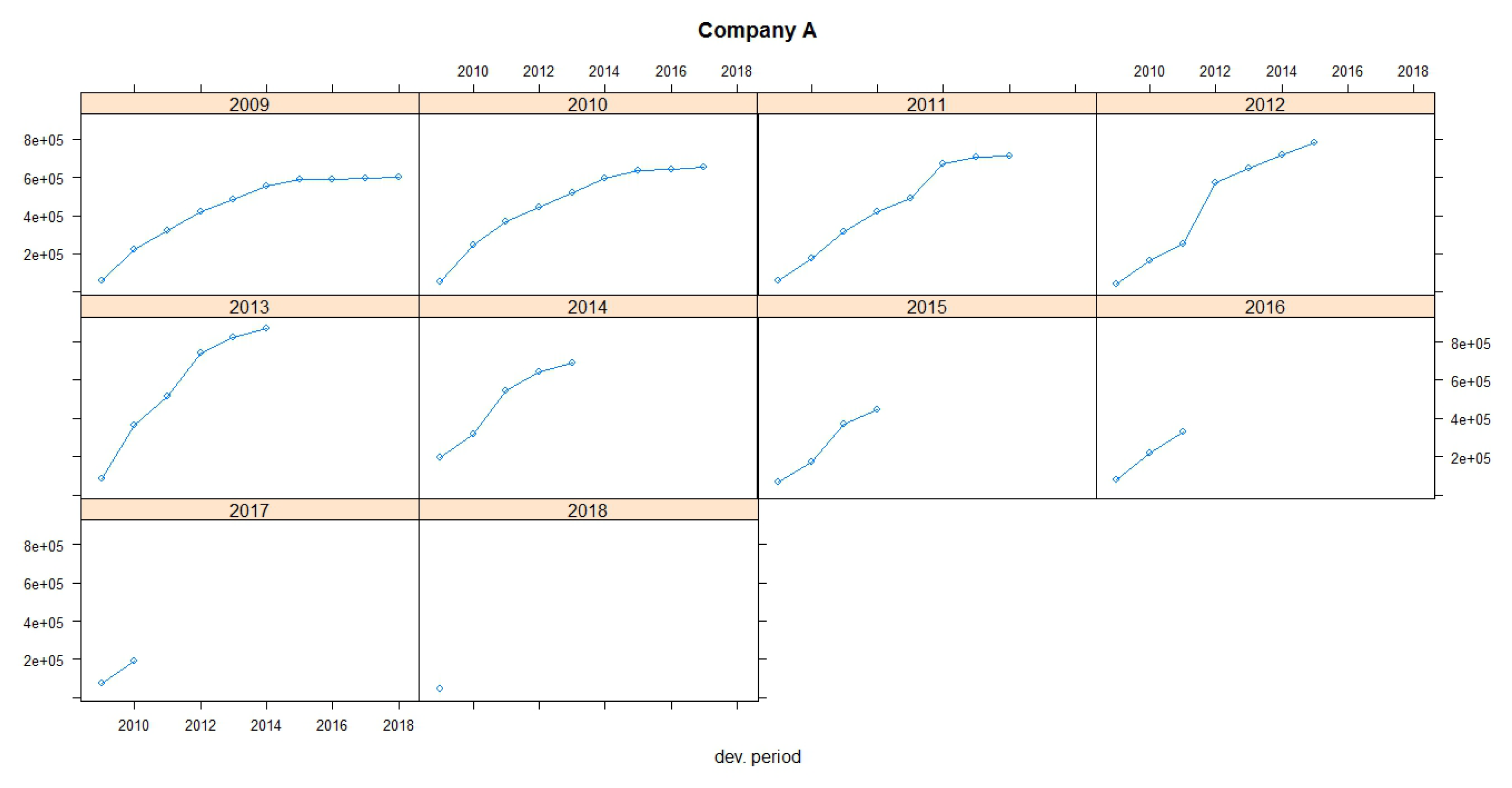
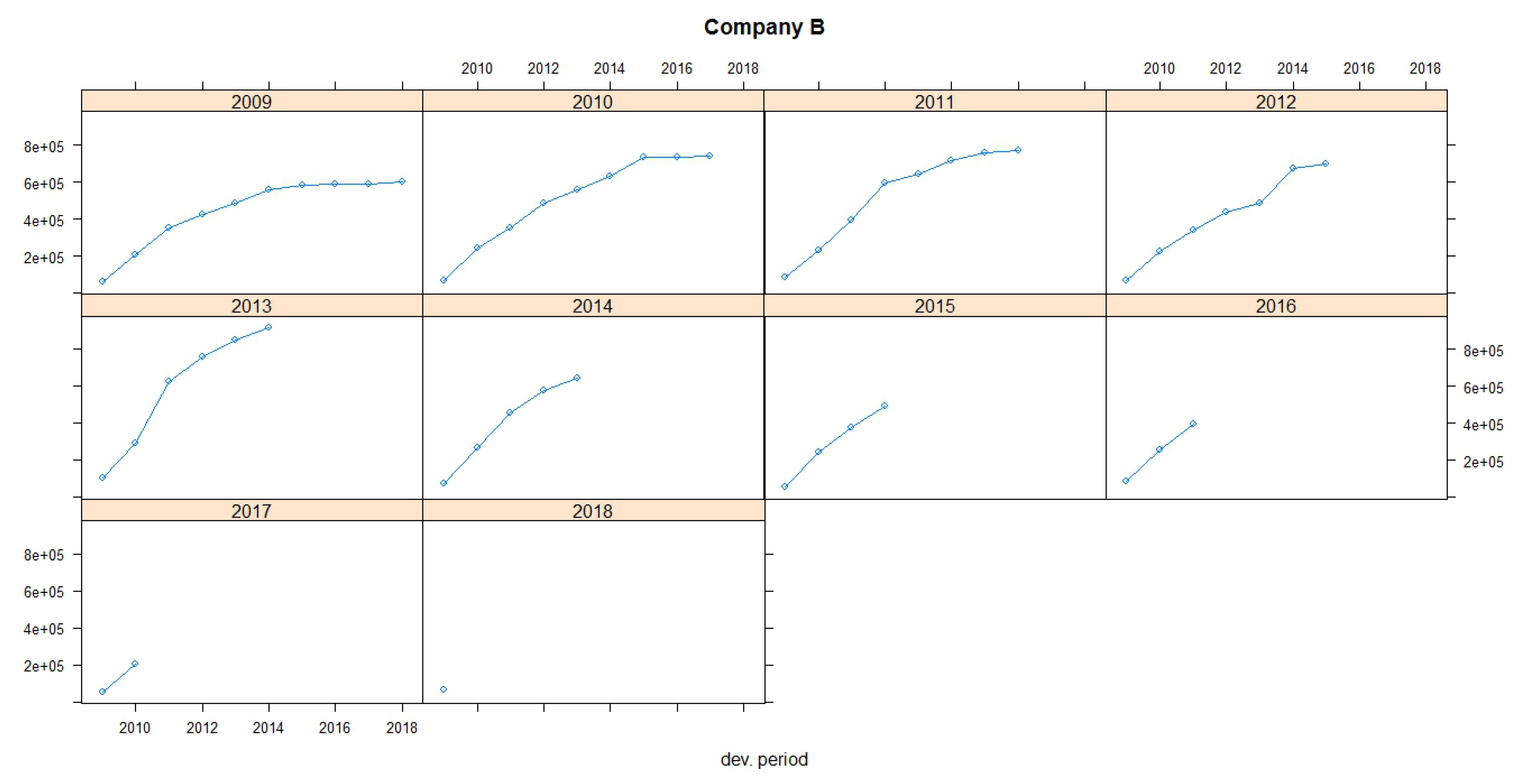
Table 5). This is commonly observed in motor business where claims are settled many years later, especially when accidents with large compensations (such as partial or total disability, deaths, etc.) are observed. This can also be observed in accident year 2008 where a large amount is observed at the last known development year (13,809). We have a similar situation for the run-off triangle for Company B, but not to that extent as for Company A. For Company B, the data of the triangle seem to be more stable. Moreover, the premiums of the companies by accident year are presented at the run-off triangles. For the implementation of the dataset, we divided the payments by exposures for each year of business before the analysis was carried out.
The number of exposures (counts of incurred losses) for each accident year is also provided (see Table 6 and Table 7) for each lines of business.
If we were trying to calculate the expected value of the reserve run-off, we could simply calculate the expected value for each line of business separately and add all the expectations together. However, when we quantify a value other than the mean, such as a quantile, we cannot simply sum across the lines of business. In such a case, we would overstate the aggregate reserve need.
Remark 3.
The only time the sum of a θ th quantile would be appropriate for the aggregate reserve indication is when all the lines of business are fully correlated with each other which is of course a highly unlikely situation.
Figure 1 and Figure 2 show claims development charts of Companies A and B, respectively, with individual panels for each origin period. Chain Ladder loss development factors for each company are also presented in 
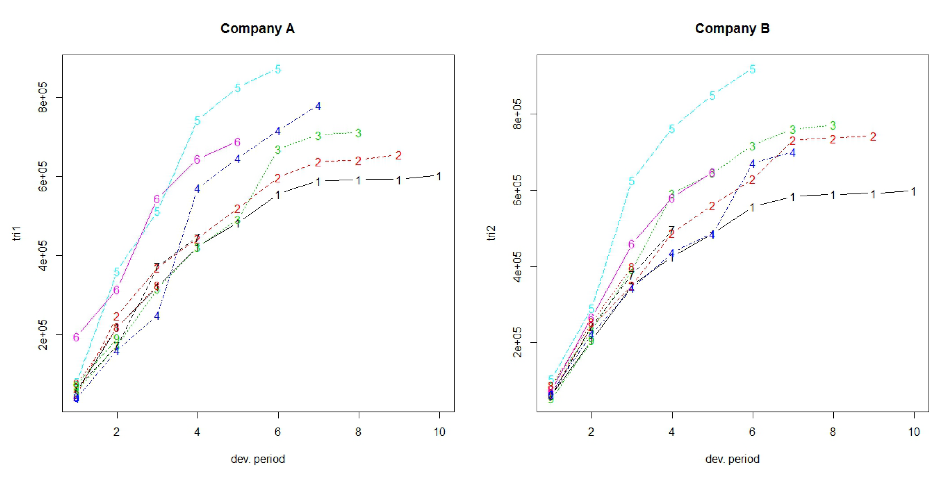
Table 5. According to the claims development chart, we observe that the patterns of Companies A and B appear similar (see Figure 3).
Table 8 and Table 9 display the values of reserves and ultimate paid claims based on individual quantile regression method, for Companies A and B, respectively, for different quantiles. Loss ratios for each quantile are also provided at the end of each of the Tables. Table 10 and Table 11 display the values of reserves and ultimate paid claims based on longitudinal quantile regression method, for Companies A and B, respectively, for different quantiles.
Loss ratios ( L R ) for motor car insurance typically range from 40% to 60%. In this case, insurance companies are collecting more premiums than the amount paid in claims. Loss ratio is considered as one of the tools which explains a company’s suitability for coverage. A high loss ratio means is considered bad, which leads to bad financial health because the insurance company may not collect enough premiums to pay claims and expenses while also making a reasonable profit.
Table 12 provides the values of reserves based on the individual quantile regression (IQR) and based on longitudinal quantile regression (LQR). To examine the role of dependence, it is important to calculate the reserves for each IQR, and then use the sum to compare it with the sum of the run-off triangles resulting from the LQR (last line of Table 12).
Applying individual quantile regression, a higher quantile leads to larger total reserve. Nevertheless, for Company A, quantiles over 95% provide equal values of reserves, while, for Company B, quantiles over 90% provide equal values of reserves. The longitudinal algorithm gives different estimations for each quantile. Applying longitudinal quantile regression, the estimated ultimate reserves for both Companies A and B are smaller than the sum of individual estimated reserves for each of Companies A and B based on individual quantile regression.

5.2. Comparison Criteria

For model comparison, four criteria, namely the root mean squared error (RMSE), the percentage total (PT), the mean absolute error (MAE), and the mean absolute percentage error (MAPE), were used.
RMSE is a measure of accuracy and is useful for comparing different models for a particular dataset (Hyndman and Koehler 2006). RMSE is the square root of the average of squared errors. The effect of each error on RMSE is proportional to the size of the squared error. Thus, larger errors have a disproportionately large effect on RMSE. Consequently, RMSE is sensitive to outliers (Pontius et al 2008; Willmott and Matsuura 2006).
RMSE for one triangle and for many run-off triangles is given, respectively, by
R M S E = 1 m i = 1 n j = 1 n i + 1 ( y i j y ^ i j ) 2 1 / 2 a n d R M S E N = 1 m N k = 1 N i = 1 n j = 1 n i + 1 ( y i j y ^ i j ) 2 1 / 2 ,
where m = n + 1 2 represents the total number of the known incremental data (the left upper triangle) and k is the counter for each triangle.
The percentage total (PT) was also a comparison criterion, which is defined for one and for many triangles, respectively, as
P T = i = 1 n j = 1 n i + 1 y ^ i j i = 1 n j = 1 n i + 1 y i j a n d P T N = k = 1 N i = 1 n j = 1 n i + 1 y ^ i j k = 1 N i = 1 n j = 1 n i + 1 y i j .
RMSE and PT measure the model-fit with respect to observations, where a PT value closer to 100 is accepted, while, for RMSE, we prefer the smallest values.
According to the comparison criteria, the longitudinal algorithm provides the smaller RMSE when using the 75% quantile, resulting to better fit of the data. Thus, a combination of different companies or lines of business provides a better estimation of the total reserve. In case of using the PT criterion, we take exactly the same results and the 75% quantile produces the best fit. If we make estimations separately, the suggested models for both triangles use quantiles below 75% which means weak prudence (Table 13).
The MAE calculates the average amount of the errors by computing the absolute differences between prediction and actual observation divided by the total number of the observations. The lower the value of MAE is, the better the model fits.
Finally, the MAPE is the average of absolute percentage errors. MAPE has the significant disadvantage of producing infinite or undefined values when the actual values are zero or close to zero (Kim and Kim 2016). If the actual values are very small, then MAPE yields extremely large percentage errors (outliers).
The MAE criterion for single run-off triangle and the total MAE for N run-off triangles is calculated, respectively, by
M A E = 1 m i = 1 n j = 1 n i + 1 y i j y i j ^ a n d M A E N = 1 m N k = 1 N i = 1 n j = 1 n i + 1 y i j k y i j k ^ .
The MAPE criterion for single run-off triangle and the total MAPE for N run-off triangles, is given, respectively, by
M A P E = 100 % m i = 1 n j = 1 n i + 1 | y i j y i j ^ y i j | a n d M A P E N = 100 % m N k = 1 N i = 1 n j = 1 n i + 1 | y i j k y i j k ^ y i j k | .
For the MAPE and MAE criteria, the smallest values indicate the best fit. The computations of the values for each criterion are given in Table 14. According to the MAE criterion, the 60% quantile is the suggested value to be used, while, based on MAPE, the 50% quantile is the most appropriate. Nevertheless, the difference between the MAE values for 50% and 60% is not so big, which means that 60% could also be a good choice.
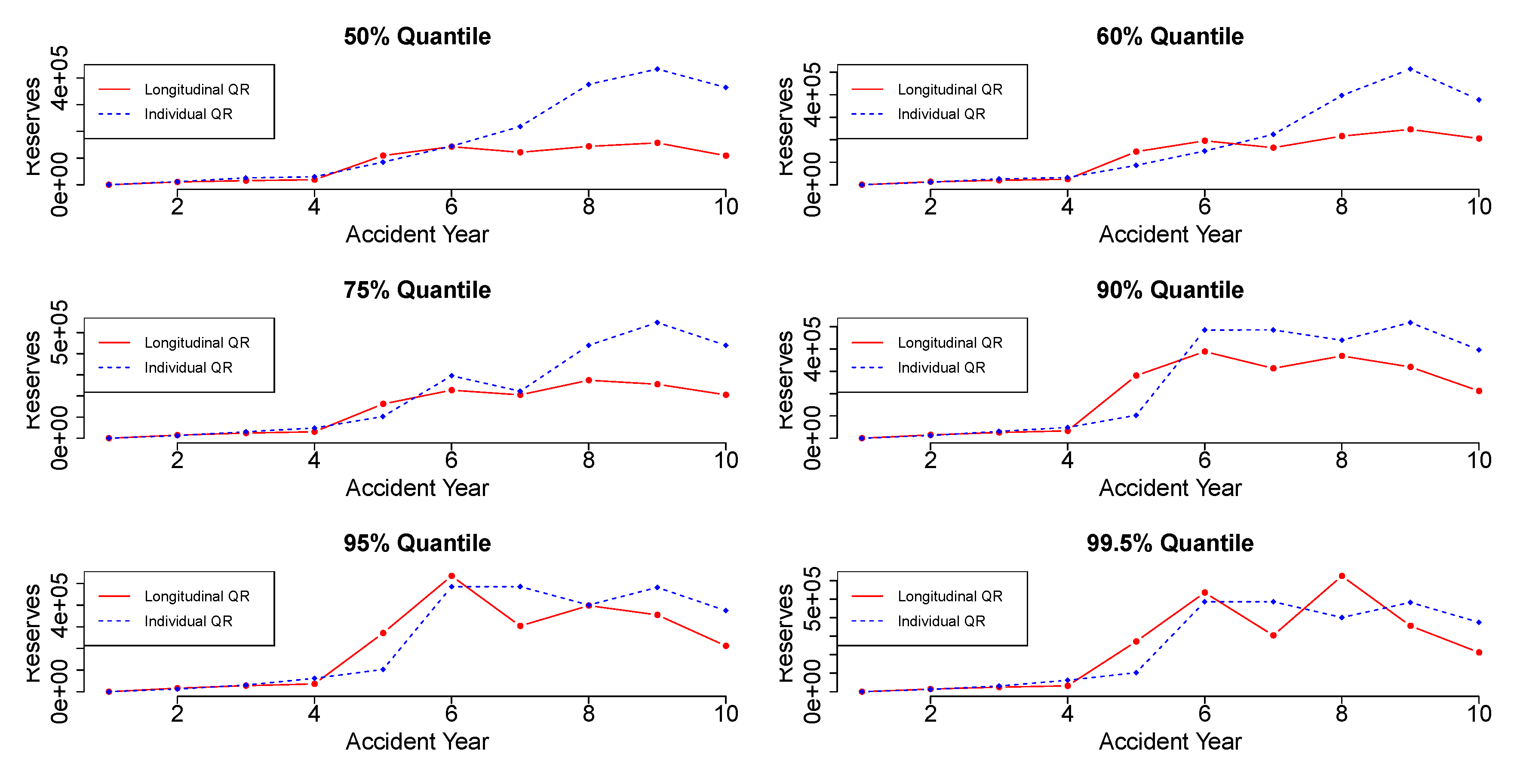
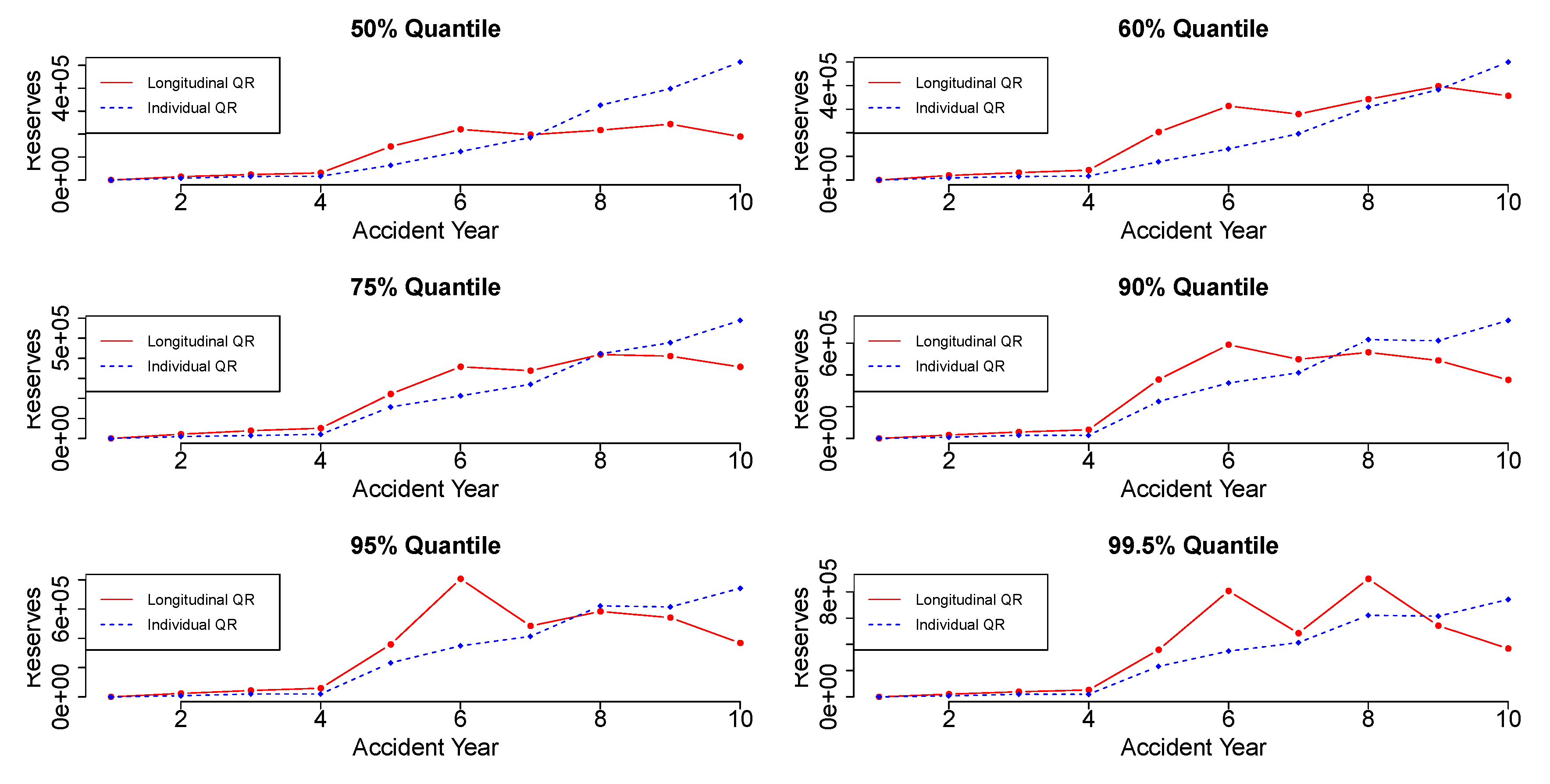
Figure 4 and Figure 5 display the reserve estimation for each accident year using the individual quantile regression and the longitudinal quantile regression. Each plot provides the reserve values in different quantiles for each accident year.
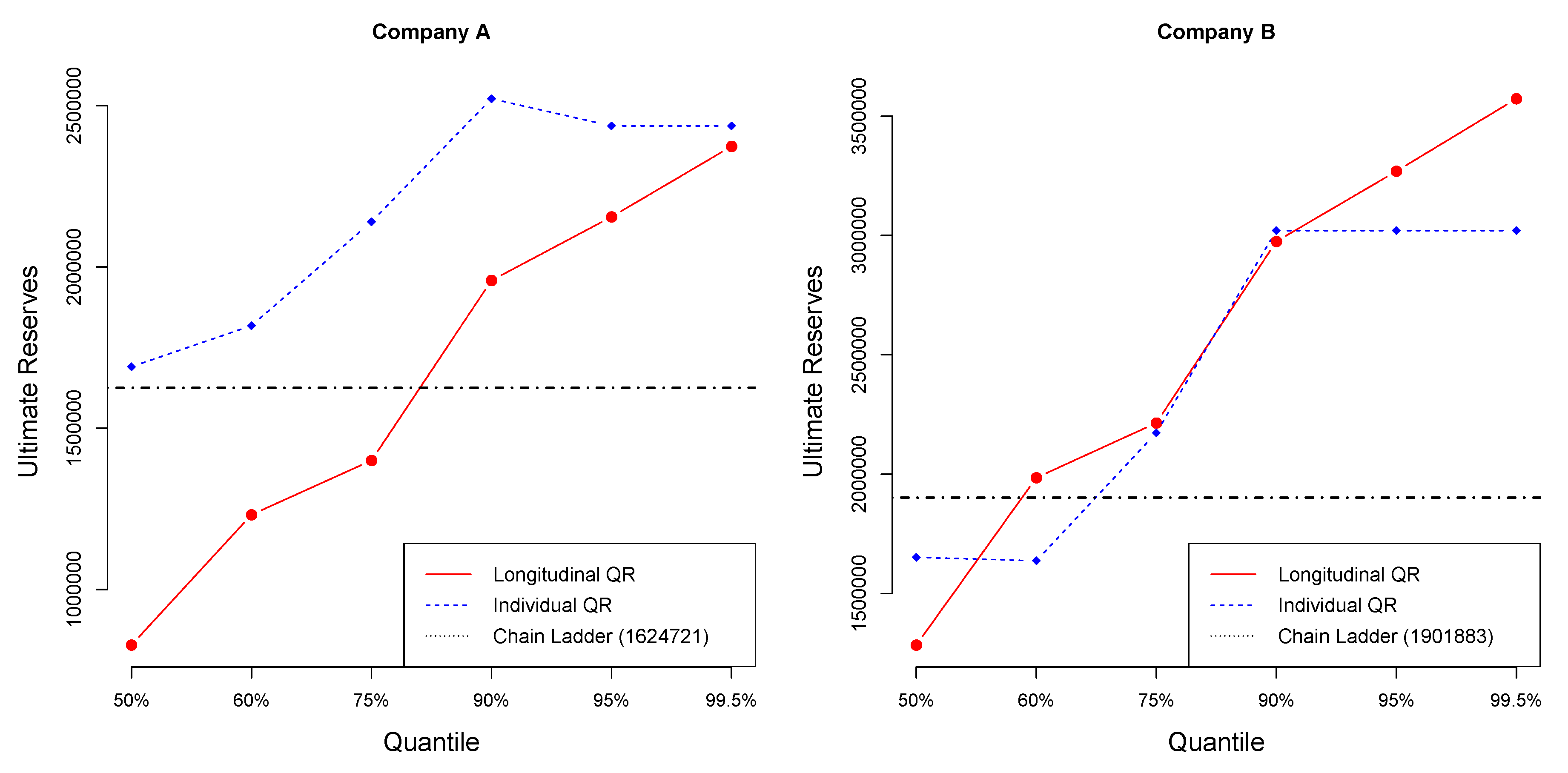
Figure 6 illustrates the values of the ultimate reserves, for different quantiles, based on the individual and the longitudinal quantile regression models, in comparison to the ultimate reserves based on the Chain Ladder method for Companies A and B. The ultimate reserves based on the Chain Ladder estimation for Company A is 1,624,721 and for Company B is 1,901,883. More specifically, for Company A, the Chain Ladder reserve value coincides with the individual quantile regression reserve value at 50-quantile, and with the longitudinal quantile regression reserve value around the 80-quantile. For Company B, the Chain Ladder reserve value coincides with the individual quantile regression reserve value around 50-quantile, and with the longitudinal quantile regression reserve value around the 60-quantile.

6. Risk Capital Requirement and Risk Margin

Solvency II and IFRS bring some significant changes, particularly in relation to the estimation of insurance liabilities. Generally, the Probability of Sufficiency is a measure of solvency in liability valuation (DalMoro and Krvavych 2017):
  • Probability of sufficiency below 50% indicates that the technical provisions are set below the central estimate, which leads to an under-reserved position.
  • Probability of sufficiency with values between 50% and 60% indicates that the technical provisions are approximately at the level of central estimate, which leads to weak prudence.
  • For values of probability of sufficiency around 75%, the technical provisions are above the central estimate, which leads to adequate prudence.
  • Finally, if the probability of sufficiency is above 75%, the technical provisions are enough to lead to strong prudence.

Risk Margin

Based on Solvency II directive, risk margin represents the potential costs to transfer the insurance obligations to a third party and it is calculated based on the cost-of-capital (CoC) method. Solvency II considers risk over a one-year time horizon.
According to this approach, when the capital requirements for each future year are given, the risk margin is equal to the sum of the discounted costs of capital, which are the capital requirements multiplied by the cost-of-capital rate (6%). The risk margin (RM) is exclusively based on the solvency capital requirement (SCR) estimation and according to the cost-of-capital (CoC) methodology is calculated as follows (CEIOPS 2009):
R M = t 0 S C R ( t ) ( 1 + r t ) t + 1 × C o C = t 0 V a R 99.5 % ( R t ) m e a n ( R t ) ( 1 + r t ) t + 1 × C o C ,
where R t is the estimated reserve for the accident year t , r t is the risk-free rate for maturity, S C R ( t ) is the Solvency Capital Requirement for the accident year t , and C o C is the cost of capital rate. The solvency capital requirement is the difference between the 99.5% quantile and the 50% quantile of the reserves. The cost of capital is 6% (as Solvency II suggests) and we suppose that the risk-free rate for maturity is r t = 1 % for all accident years (the real risk-free rate for maturity is given by EIOPA).
Along with the best estimate (BE), risk margin makes up the technical provisions and ensures that their value is equivalent to the amount that an (re)insurer would be expected to require in order to take over and meet the insurance obligations. Generally, risk margin increases the value of the technical provisions from the BE up to an amount which is equivalent to a theoretical level needed to transfer obligations to another (re)insurer. Risk margin represents what an (re)insurer would have to pay to the market to take on the BE liabilities. When the market takes on your BE liabilities, they will have to set aside capital to cover the SCR. Therefore, holding the SCR incurs a cost. Risk margin represents this cost. Dong et al. (2015) showed how one can provide an accurate estimation of risk margin and hence provision, instead of estimating the mean and then applying a risk margin. Their method is more robust when the data are heavy tailed. Their approach has been used for the univariate quantile regression model and is suitable for a simple line of business (single run-off triangle).
Table 15 presents the calculated risk margins for each individual line of business (Companies A and B), based on the univariate quantile regression model and Table 16 presents the corresponding risk margin for each individual line of business based on our longitudinal model.
Finally, Table 17 presents the calculated risk margins based on the bootstrap method and the resulting Figure 7 and Figure 8 illustrate: (a) the histograms of total simulated IBNRs; (b) the empirical cumulative distribution functions of IBNRs; (c) the simulated ultimate claim cost against ultimate claim cost; and (d) the latest actual incremental claims cost for the latest available calendar period against latest incremental claims, for Companies A and B, respectively.
From histograms and the empirical cumulative distribution functions, we observe that the IBNRs may follow distributions with positive skewness. We also observe that the simulated data may not follow the same trend as the actual data (specifically in Company B). It indicates that the original data might have some trends that are not reflected in the model.
Remark 4.
If the distribution of the reserves were known, then the mean of this distribution would be the BE, i.e., the amount to be paid as compensation to the beneficiaries. Nevertheless, this distribution is not known and for that reason many methodologies are used to estimate the BE such as the bootstrap method. In case of quantile regression models, a specific quantile, which provides estimations close to the mean, would be used to estimate the BE. For that reason, we use the 50% quantile, but a larger one could be used especially for long tail distributions.

7. Concluding Remarks

We propose quantile regression for longitudinal data in the framework of a general multivariate loss reserving model. Our model considers a combination of the between and within lines of business, taking into account the correlations and variation of run-off triangles. We investigated a general insurance portfolio that consists of two correlated subportfolios (two auto run-off triangles). The least squares estimators investigated only changes in the mean, while the quantile regression characterized a particular point of a distribution, which provides a more complete description of the entire shape of the claims distribution. According to Solvency II and IFRS, the solvency capital requirement (SCR) was provided based on the best estimate (BE) and, in the sequel, the overall risk margin (RM), based on the cost-of-capital (CoC) methodology, was calculated.

Author Contributions

I.B., G.P. contributed equally to this work. All authors have read and agreed to the published version of the manuscript.

Funding

This research received no external funding.

Acknowledgments

This work was partly supported by the University of Piraeus Research Center.

Conflicts of Interest

The authors declare no conflict of interest.

References

  1. Abdallah, Anas, Jean-Philippe Boucher, and Hélène Cossette. 2015. Modeling Dependence between Loss Triangles with Hierarchical Archimedean Copulas. ASTIN Bulletin 45: 577–99. [Google Scholar] [CrossRef] [Green Version]
  2. Ajne, Björn. 1994. Additivity of chain–ladder projections. ASTIN Bulletin 24: 313–8. [Google Scholar] [CrossRef] [Green Version]
  3. Antonio, Katrien, and Jan Beirlant. 2006. Actuarial statistics with generalized linear mixed models. Insurance: Mathematics and Economics 75: 643–76. [Google Scholar] [CrossRef]
  4. Avanzi, Benjamin, Greg Taylor, Phuong Anh Vu, and Bernard Wong. 2016a. Stochastic loss reserving with dependence: A flexible multivariate Tweedie approach. Insurance: Mathematics and Economics 71: 63–78. [Google Scholar] [CrossRef] [Green Version]
  5. Avanzi, Benjamin, Greg Taylor, and Bernard Wong. 2016b. Correlations between insurance lines of business: An illusion or a real phenomenon? Some methodological considerations. ASTIN Bulletin 46: 225–63. [Google Scholar] [CrossRef] [Green Version]
  6. Avanzi, Benjamin, Greg Taylor, and Bernard Wong. 2018. Common Shock Models for Claim Arrays. ASTIN Bulletin 48: 1109–36. [Google Scholar] [CrossRef] [Green Version]
  7. Barnett, Glen, and Ben Zehnwirth. 2000. Best estimates for reserves. Proceedings of the Casualty Actuarial Society 87: 245–321. [Google Scholar]
  8. Bartlett, M. S. 1951. An inverse matrix adjustment arising in discriminant analysis. Annals of Mathematical Statistics 22: 107–11. [Google Scholar] [CrossRef]
  9. Bermúdez, Lluis, Antoni Ferri, and Montserrat Guille. 2013. A Correlation Sensitivity Analysis for non-life underwriting risk module SCR. ASTIN Bulletin 43: 21–37. [Google Scholar] [CrossRef] [Green Version]
  10. Braun, Christian. 2004. The prediction error of the chain ladder method applied to correlated run-off triangles. ASTIN Bulletin 34: 399–423. [Google Scholar] [CrossRef] [Green Version]
  11. Brown, Bruce Maxwell, and You-Gan Wang. 2005. Standard errors and covariance matrices for smoothed rank estimators. Biometrika 92: 149–58. [Google Scholar] [CrossRef]
  12. Buchinsky, Moshe. 1998. Recent advances in regression models: A practical guideline for empirical research. The Journal of Human Resources 33: 88–126. [Google Scholar] [CrossRef]
  13. CEIOPS. 2009. Advice for Level 2 Implementing Measures on Solvency II: Technical Provisions, Article 86 (d). Frankfurt: CEIOPS. [Google Scholar]
  14. Chan, Jeniffer S. K., S. T. Boris Choy, and Udi E. Makov. 2008. Dynamic and robust models for loss reserves using generalized-t distribution. ASTIN Bulletin 38: 207–30. [Google Scholar] [CrossRef] [Green Version]
  15. Chen, Li, Lee-Jen Wei, and Michael I. Parzen. 2004. Quantile regression for correlated observations. In Proceedings of the Second Seattle Symposium in Biostatistics. Lecture Notes in Statistics. New York: Springer, vol. 179, pp. 51–69. [Google Scholar]
  16. Christofides, S. 1990. Regression models based on log-incremental payments. In Claims Reserving Manual 2. London: Institute of Actuaries. [Google Scholar]
  17. Clark, David R. 2006. Variance and covariance due to inflation. CAS Forum 11: 61–95. [Google Scholar]
  18. Dal Moro, Eric, and Yuriy Krvavych. 2017. Probability of sufficiency of solvency II reserve risk margins: Practical approximations. ASTIN Bulletin 47: 737–85. [Google Scholar] [CrossRef]
  19. De Jong, Piet. 2012. Modeling Dependence between Loss Triangles. North American Actuarial Journal 16: 74–86. [Google Scholar] [CrossRef]
  20. Diggle, Peter J., Patrick J. Heagerty, Kung-Yee Liang, and Scott L. Zeger. 2002. Analysis of Longitudinal Data. New York: Oxford University Press. [Google Scholar]
  21. Dong, Alice X. D., Jennifer S. K. Chan, and Gareth W. Peters. 2015. Risk margin quantile function via parametric and non-parametric bayesian approaches. ASTIN Bulletin 45: 503–50. [Google Scholar] [CrossRef]
  22. Fu, Liya, and You-Gan Wang. 2012. Quantile regression for longitudinal data with a working correlation model. Computational Statistics & Data Analysis 56: 2526–38. [Google Scholar]
  23. Gesmann, M., D. Murphy, Y. Zhang, A. Carrato, M. Wuthrich, F. Concina, and E. Dal Moro. 2018. ChainLadder: Statistical Methods and Models for Claims Reserving in General Insurance. R package version 0.2.9. Available online: https://CRAN.R-project.org/package=ChainLadder (accessed on 27 May 2019).
  24. Gilchrist, Warren G. 2000. Statistical Modelling with Quantile Functions. London: Chapman & Hall. [Google Scholar]
  25. Harrison, David A., and Charles L. Hulin. 1989. Investigations of absenteeism: Using event-history models to study the absence-taking process. Journal of Applied Psychology 74: 300–16. [Google Scholar] [CrossRef]
  26. Holmberg, Randall D. 1994. Correlation and the measurement of loss reserve variability. CAS Forum 1: 247–78. [Google Scholar]
  27. Hubert, Mia, Tim Verdonck, and Özlem Yorulmaz. 2017. Fast robust SUR with economical and actuarial applications. Statistical Analysis and Data Mining 10: 77–88. [Google Scholar] [CrossRef]
  28. Hudecová, Šárka, and Michal Pešta. 2013. Modeling dependencies in claims reserving with GEE. Insurance: Mathematics and Economics 53: 786–94. [Google Scholar] [CrossRef] [Green Version]
  29. Hyndman, Rob J., and Anne B. Koehler. 2006. Another look at measures of forecast accuracy. International Journal of Forecasting 22: 679–88. [Google Scholar] [CrossRef] [Green Version]
  30. Jung, Sin-Ho. 1996. Quasi-likelihood for median regression models. Journal of the American Statistical Association 91: 251–7. [Google Scholar] [CrossRef]
  31. Kim, Sungil, and Heeyoung Kim. 2016. A new metric of absolute percentage error for intermittent demand forecasts. International Journal of Forecasting 32: 669–79. [Google Scholar] [CrossRef]
  32. Koenker, Roger, and Gilbert Basset. 1982. Robust Tests for Heteroscedasticity Based on Regression Quantiles. Econometrica 50: 43–61. [Google Scholar] [CrossRef] [Green Version]
  33. Koenker, Roger, and Vasco D’Orey. 1994. A remark on algorithm AS229: Computing dual regression quantiles and regression rank scores. Applied Statistics 43: 410–4. [Google Scholar] [CrossRef]
  34. Koenker, Roger. 2005. Quantile Regression. Cambridge: University Press. [Google Scholar]
  35. Koenker, Roger. 2018. Quantreg: Quantile Regression. R Package Version 5.36. Available online: https://CRAN.R-project.org/package=quantreg (accessed on 13 December 2019).
  36. Kremer, Erhard. 2005. The correlated chain-ladder method for reserving in case of correlated claims developments. Blatter DGVFM 27: 315–22. [Google Scholar] [CrossRef]
  37. Kuang, Di, Bent Nielsen, and Jens Perch Nielsen. 2011. Forecasting in an Extended Chain-Ladder–Type Model. The Journal of Risk and Insurance 78: 345–59. [Google Scholar] [CrossRef] [Green Version]
  38. Mack, Thomas. 1993. Distribution-free calculation of the standard error of chain-ladder reserve estimates. ASTIN Bulletin 23: 213–25. [Google Scholar] [CrossRef] [Green Version]
  39. Merz, Michael, and Mario Wüthrich. 2008a. Prediction error of the chain ladder reserving method applied to correlated run off trapezoids. Annals of Actuarial Science 2: 25–50. [Google Scholar] [CrossRef] [Green Version]
  40. Merz, Michael, and Mario Wüthrich. 2008b. Prediction error of the multivariate chain ladder reserving method. North American Actuarial Journal 12: 175–97. [Google Scholar] [CrossRef]
  41. Merz, Michael, Mario Wüthrich, and Enkelejd Hashorva. 2012. Dependence modelling in multivariate claims run-off triangles. Annals of Actuarial Science 7: 3–25. [Google Scholar] [CrossRef] [Green Version]
  42. Pang, Lei, Wenbin Lu, and Huixia Judy Wang. 2012. Variance estimation in censored quantile regression via induced smoothing. Computational Statistics and Data Analysis 56: 785–96. [Google Scholar] [CrossRef] [Green Version]
  43. Parzen, M. I., L. J. Wei, and Z. Ying. 1994. A resampling method based on pivotal estimating functions. Biometrika 81: 341–50. [Google Scholar] [CrossRef]
  44. Peremans, Kris, Stefan Van Aelst, and Tim Verdonck. 2018. A robust general multivariate chain ladder method. Risks 6: 108. [Google Scholar] [CrossRef] [Green Version]
  45. Pešta, Michal, and Ostap Okhrin. 2014. Conditional least squares and copulae in claims reserving for a single line of business. Insurance: Mathematics and Economics 56: 28–37. [Google Scholar] [CrossRef] [Green Version]
  46. Pitt, David G. W. 2006. Regression quantile analysis of claim termination rates for income protection insurance. Annals of Actuarial Science 1: 345–57. [Google Scholar] [CrossRef] [Green Version]
  47. Pontius, Robert Gilmore, Olufunmilayo Thontteh, and Hao Chen. 2008. Components of information for multiple resolution comparison between maps that share a real variable. Environmental Ecological Statistics 15: 111–42. [Google Scholar] [CrossRef]
  48. Pröhl, Carsten, and Klaus D. Schmidt. 2005. Multivariate Chain-Ladder. Dresdner Schriften zur Versicherungsmathematik. Available online: https://www.math.tu-dresden.de/sto/schmidt/dsvm/dsvm2005-3.pdf (accessed on 13 December 2019).
  49. Quarg, Gerhard, and Thomas Mack. 2004. Munich chain ladder. Blatter DGVFM 4: 597–630. [Google Scholar] [CrossRef]
  50. Radtke, Michael, Klaus D. Schmidt, and Anja Schnaus. 2012. Handbook on Loss Reserving. EAA Lecture Notes. European Actuarial Academy. Berlin: Springer. [Google Scholar]
  51. Schmidt, Klaus D. 2006. Optimal and additive loss reserving for dependent lines of business. Paper presented at 2006 CAS Casualty Loss Reserve Seminar, Atlanta, GA, USA, September 11–12; pp. 319–51. [Google Scholar]
  52. Searle, Shayle R., George Casella, and Charles E. McCulloch. 1992. Variance Components. New York: John Wiley and Sons. [Google Scholar]
  53. Shi, Peng, and Edward Frees. 2011. Dependent loss reserving using copulas. ASTIN Bulletin 41: 449–86. [Google Scholar]
  54. Shi, Peng, Sanjib Basu, and Glenn G. Meyers. 2012. A Bayesian log-normal model for multivariate loss reserving. North American Actuarial Journal 16: 29–51. [Google Scholar] [CrossRef]
  55. Stoner, Julie A., and Brian G. Leroux. 2002. Analysis of clustered data: A combined estimating equations approach. Biometrika 89: 567–78. [Google Scholar] [CrossRef]
  56. Taylor, Greg, and Grainne Mcguire. 2005. Synchronous bootstrapping of seemingly unrelated regressions. Paper presented at the 36th International ASTIN Colloquium, ETH, Zurich, September 4–7. [Google Scholar]
  57. Taylor, Greg, and Grainne Mcguire. 2007. A synchronous bootstrap to account for dependencies between lines of business in the estimation of loss reserve prediction error. North American Actuarial Journal 11: 70–88. [Google Scholar] [CrossRef]
  58. Taylor, Gregory. 2000. Loss Reserving—An Actuarial Perspective. Norwell: Kluwer Academic Publishers. [Google Scholar]
  59. Wang, You-Gan, Quanxi Shao, and Min Zhu. 2009. Quantile regression without the curse of unsmoothness. Computational Statistics and Data Analysis 53: 3696–705. [Google Scholar] [CrossRef]
  60. Willmott, Cort, and Kenji Matsuura. 2006. On the use of dimensioned measures of error to evaluate the performance of spatial interpolators. International Journal of Geographic Information Science 20: 89–102. [Google Scholar] [CrossRef]
  61. Wüthrich, Mario, and Michael Merz. 2008. Stochastic Claims Reserving Methods in Insurance. Hoboken: Wiley Finance. [Google Scholar]
  62. Wüthrich, Mario V. 2010. Accounting Year Effects Modeling in the Stochastic Chain Ladder Reserving Method. North American Actuarial Journal 14: 235–55. [Google Scholar] [CrossRef]
  63. Yin, Guosheng, and Jianwen Cai. 2005. Quantile regression models with multivariate failure time data. Biometrics 61: 151–61. [Google Scholar] [CrossRef]
  64. Zehnwirth, Ben, and Glen Barnett. 2001. Reserving for multiple excess layers. Paper presented at the ASTIN Colloquium at the ASTIN Colloquium, Washington, DC, USA, July 8–11. [Google Scholar]
  65. Zhang, Yanwei, Vanja Dukic, and James Guszcza. 2012. A Bayesian non-linear model for forecasting insurance loss payments. Journal Royal Statistical Society A 175: 637–56. [Google Scholar] [CrossRef]
  66. Zhang, Yanwei. 2010. A general multivariate chain ladder model. Insurance: Mathematics and Economics 46: 588–99. [Google Scholar] [CrossRef]
Figure 1. Claims development chart of Company A with individual panels for each origin period.
Risks 08 00014 g001
Figure 2. Claims development chart of Company B with individual panels for each origin period.
Risks 08 00014 g002
Figure 3. Claims development chart of the triangles with one line per origin period.
Risks 08 00014 g003
Figure 4. Reserves estimation for individual QR and longitudinal QR (Company A).
Risks 08 00014 g004
Figure 5. Reserves estimation for individual QR and longitudinal QR (Company B).
Risks 08 00014 g005
Figure 6. Ultimate reserves for individual QR and longitudinal QR.
Risks 08 00014 g006
Figure 7. Bootstrap graphs for Company A.
Risks 08 00014 g007
Figure 8. Bootstrap graphs for Company B.
Risks 08 00014 g008
Table 1. Representation of N run-off triangles.
AccidentDevelopment Year j
Yearr12 j I 1I
1 Y 11 Y 12 Y 1 j Y 1 , I 1 Y 1 I
2 Y 21 Y 22 Y 2 j Y 2 , I 1
r Y r 1 Y r , I + 1 r
I Y I 1
Table 2. N Run-off Triangles in a Longitudinal Form.
SubjectObservationResponseCovariates
11 y 11 x 111 x 11 p
12 y 12 x 121 x 12 p
1 n 1 y 1 n 1 x 1 n 1 1 x 1 n 1 p
N1 y N 1 x N 11 x N 1 p
N2 y N 2 x N 21 x N 2 p
N n N y N n N x N n N 1 x N n N p
Table 3. Motor triangle and premiums for Company A.
AccidentDevelopment Year
Year12345678910Premium
200758,134162,688101,105100,96461,59171,00934,024274664610,1901,051,637
200851,437197,139120,64174,80776,77177,27639,070439613,809 1,190,965
200957,906116,191143,953103,88370,760177,19435,3416088 1,327,568
201040,352121,83788,389320,42975,12770,19063723 1,418,348
201182,227279,591151,260230,29382,37847,315 1,504,056
2012196,417119,755228,49999,89444,266 1,580,233
201367,161107,098198,25275,172 1,619,382
201478,293141,865106,150 1,727,540
201574,472118,886 1,820,104
201643,281 1,883,017
Table 4. Motor triangle and premiums for Company B.
AccidentDevelopment Year
Year12345678910Premium
200763,078143,002144,23575,00760,77570,80427,5084757317263851,633,833
200865,567177,292107,870137,30572,74168,708102,86443356107 1,675,707
200987,394146,346158,876199,84653,16172,76442,91510,898 1,636,855
201070,017153,893119,02893,77149,600185,68928,331 1,689,715
2011104,638186,326335,477136,85787,94169,248 1,649,386
201276,390190,629192,606121,70466,297 1,712,587
201358,620184,557135,174118,180 2,105,361
201487,845166,511145,385 2,265,432
201553,616152,751 1,976,188
201662,904 1,351,719
Table 5. Chain ladder: loss development factors.
Company0–11–22–33–44–55—66-77–88–9
A2.93241.60601.37371.12651.14911.06771.00681.01171.0171
B3.25021.68221.30421.11881.15411.07821.00961.00691.0107
Table 6. Counts of incurred claims for Company A.
AccidentDevelopment Year
Year12345678910
200711827224116910310671435
2008134287235192121117841413
20091292542671931101368016
2010872552181521118652
201114828527721212794
2012108255227185103
2013129215220150
2014128277234
2015122236
201694
Table 7. Counts of incurred claims for Company B.
AccidentDevelopment Year
Year12345678910
2007139286276170137140741586
2008143337258224158158902013
20091512733102391451358111
201013828527318212212770
2011161372349282185129
2012131327297237150
2013144345284222
2014146337295
2015130301
2016155
Table 8. Reserves and ultimate claims of Company A based on Individual Quantile Regression.
AccidentQuantile 50%Quantile 60%Quantile 75%Quantile 90%Quantile 95%Quantile 99.5%
YearReservesUltimateReservesUltimateReservesUltimateReservesUltimateReservesUltimateReservesUltimate
20070603,0970603,0970603,0970603,0970603,0970603,097
200811,702667,04911,496666,84312,348667,69512,348667,69512,348667,69512,348667,695
200925,522736,83825,770737,08530,734742,05030,734742,05030,734742,05030,734742,050
201030,123810,17132,114812,16148,436828,48448,436828,48461,841841,88861,841841,888
201184,962958,02786,226959,291102,917975,981102,917975,981102,917975,981102,917975,981
2012144,793833,624150,033838,863295,824984,655485,5281,174,359485,5281,174,359485,5281,174,359
2013218,293665,976223,617671,300222,374670,057485,688933,370485,688933,370485,688933,370
2014376,255702,563396,658722,966439,704766,012439,675765,983400,741727,049400,741727,049
2015433,878627,236514,291707,648547,762741,119519,185712,542482,151675,508482,151675,508
2016364,632407,912377,312420,592439,462482,742396,155439,435374,632417,912374,632417,912
Total1,690,1617,012,4911,817,5167,139,8462,139,5627,461,8932,520,6667,842,9962,436,5797,758,9092,436,5797,758,909
LR46.37%47.21%49.34%51.86%51.31%51.31%
Table 9. Reserves and ultimate claims of Company B based on Individual Quantile Regression.
AccidentQuantile 50%Quantile 60%Quantile 75%Quantile 90%Quantile 95%Quantile 99.5%
YearReservesUltimateReservesUltimateReservesUltimateReservesUltimateReservesUltimateReservesUltimate
20070598,7220598,7220598,7220598,7220598,7220598,722
20087915750,7058760751,5509338752,1287642750,4317642750,4317642750,431
200915,633787,83315,012787,21314,631786,83120,011792,21120,011792,21120,011792,211
201016,638716,96916,780717,11120,452720,78319,694720,02519,694720,02519,694720,025
201164,164984,65177,249997,735156,9401,077,426232,4131,152,900232,4131,152,900232,4131,152,900
2012124,174771,801131,694779,320212,699860,326348,719996,345348,719996,345348,719996,345
2013184,956681,488196,298692,830270,111766,642413,334909,865413,334909,865413,334909,865
2014326,036725,777308,932708,673422,205821,946621,7631,021,504621,7631,021,504621,7631,021,504
2015398,134604,501382,772589,139477,907684,274614,736821,104614,736821,104614,736821,104
2016514,302577,206499,960562,864588,777651,681742,201805,105742,201805,105742,201805,105
Total1,651,9537,199,6531,637,4577,185,1562,173,0607,720,7593,020,5138,568,2133,020,5138,568,2133,020,5138,568,213
LR40.68%40.60%43.63%48.42%48.42%48.42%
Table 10. Reserves and ultimate claims of Company A based on Longitudinal Quantile Regression.
AccidentQuantile 50%Quantile 60%Quantile 75%Quantile 90%Quantile 95%Quantile 99.5%
YearReservesUltimateReservesUltimateReservesUltimateReservesUltimateReservesUltimateReservesUltimate
20070603,0970603,0970603,0970603,0970603,0970603,097
200810,465665,81213,163668,50914,614669,96114,998670,34416,354671,70114,284669,631
200915,332726,64719,519730,83424,491735,80725,753737,06927,823739,13924,671735,987
201018,773798,82024,548804,59530,472810,51933,114813,16136,000816,04731,594811,641
2011109,292982,356146,9471,020,012162,3941,035,459280,8761,153,941270,8611,143,926271,1681,144,233
2012142,717831,548195,409884,240227,356916,187388,8191,077,650534,9121,223,743535,1841,224,015
2013121,615569,298164,628612,311205,183652,866313,448761,131303,832751,515304,086751,769
2014143,793470,101216,128542,436274,426600,734369,152695,460398,023724,331624,747951,055
2015156,935350,292245,965439,323255,528448,885319,659513,016354,969548,327355,450548,807
2016108,851152,131205,266248,546205,286248,567211,902255,182211,842255,123211,977255,257
Total827,7716,150,1021,231,5726,553,9031,399,7516,722,0811,957,7207,280,0502,154,6177,476,9472,373,1617,695,491
LR40.67%43.34%44.45%48.14%49.44%50.89%
Table 11. Reserves and ultimate claims of Company B based on Longitudinal Quantile Regression.
AccidentQuantile 50%Quantile 60%Quantile 75%Quantile 90%Quantile 95%Quantile 99.5%
YearReservesUltimateReservesUltimateReservesUltimateReservesUltimateReservesUltimateReservesUltimate
20070598,7220598,7220598,7220598,7220598,7220598,722
200814,812757,60219,390762,17921,292764,08221,818764,60823,573766,36320,865763,655
200923,811796,01231,465803,66538,726810,92740,529812,73043,425815,62538,967811,168
201031,032731,36342,019742,34951,128751,45954,931755,26259,120759,45152,655752,985
2011146,1381,066,624203,3531,123,839221,6911,142,178370,2261,290,712358,2821,278,769358,6741,279,161
2012220,915868,541313,593961,219357,7661,005,392589,5091,237,135806,3401,453,966806,7471,454,373
2013197,552694,083279,346775,877337,958834,489497,873994,404484,759981,290485,153981,684
2014217,454617,195342,324742,065418,633818,374541,538941,279583,882983,622899,0211,298,762
2015243,640450,007397,190603,557410,815617,182490,441696,808541,561747,928542,253748,621
2016189,118252,022356,630419,534356,665419,569368,159431,063368,056430,960368,290431,194
Total1,284,4726,832,1721,985,3087,533,0082,214,6757,762,3752,975,0238,522,7223,268,9998,816,6983,572,6259,120,325
LR38.61%42.57%43.86%48.16%49.82%51.54%
Table 12. Estimated reserves using Individual Quantile Regression (IQR) and the Longitudinal Quantile Regression (LQR).
Quantile 50%Quantile 60%Quantile 75%Quantile 90%Quantile 95%Quantile 99.5%
Company A IQR1,690,1611,817,5162,139,5622,520,6662,436,5792,436,579
Company B IQR1,651,9531,637,4572,173,0603,020,5133,020,5133,020,513
Company A LQR827,7711,231,5721,399,7511,957,7202,154,6172,373,161
Company B LQR1,284,4721,985,3082,214,6752,975,0233,268,9993,572,625
sumIQR-sumLQR1,229,871238,092698,196608,43633,477 488,694
Table 13. RMSE and PT for Individual and Longitudinal Quantile Regression.
Root Mean Square Error (RMSE)Percentage Total (PT)
QuantileCompany ACompany BLongitudinalCompany ACompany BLongitudinal
50%457.52248.60398.0782.7890.3784.02
60%455.12244.40389.5990.2693.6693.32
75%511.97263.43388.36123.37106.04106.02
90%730.79466.38536.24158.87139.59151.32
95%693.67466.38762.02158.87139.59185.72
99.5%730.79466.38789.86158.87139.59186.01
Table 14. MAE and MAPE for Individual and Longitudinal Quantile Regression.
Mean Absolute Error (MAE)Mean Absolute Percentage Error (MAPE)
QuantileCompany ACompany BCombinedCompany ACompany BCombined
50%272.30158.31212.5338.00%27.86%31.99%
60%274.38155.00210.8939.13%27.19%32.60%
75%375.69178.86233.6362.06%33.69%39.49%
90%521.73336.46441.9393.37%66.41%84.37%
95%520.07336.46610.0092.54%66.41%83.07%
99.5%522.96336.46614.5093.53%66.41%84.38%
Table 15. Risk Margin based on Individual Quantile Regression.
Company ACompany B
Accident YearSCRCapital Charge 6%Discounted Capital ChargeSCRCapital Charge 6%Discounted Capital Charge
1% Discount Rate(1% Discount Rate)
1340,87420,45220,452383,01522,98122,981
2231,10013,86613,594287,63017,25816,919
393,71756235405259,31315,55914,955
452,55531532971208,15712,48911,769
540,74924452259170,76110,2469465
655,9633358304157,43434463121
755853352982310139123
836632201916043
9167210086000
Total825,87949553RM = 48,2971,368,68082,121RM = 79,337
Table 16. Risk Margin based on Longitudinal Quantile Regression.
Company ACompany B
Accident YearSCRCapital Charge 6%Discounted Capital ChargeSCRCapital Charge 6%Discounted Capital Charge
1% Discount Rate(1% Discount Rate)
1389,95723,39723,397511,49330,69030,690
2321,75419,30519,114436,21926,17325,914
3244,76414,68614,396368,08122,08521,650
4118,91171356925162,89697749486
573,56644144242116,99970206746
612,59875671919,94911971139
71699102962103126119
855433315503331
9000000
Total1,163,80269,828RM =68,9211,618,28997,097RM = 95,774
Table 17. Risk Margin based on Bootstrap (Poisson).
Company ACompany B
Accident YearSCRCapital Charge 6%Discounted Capital ChargeSCRCapital Charge 6%Discounted Capital Charge
1% Discount Rate(1% Discount Rate)
12,79,59216775167753699222219512797
224525814715145703625412175211567
32090051254012293287763172669251
4168286100979800213236127947042
514773488648518215192129126485
6935595614534114238485434099
763681382135998076848462289
856266337631497513245081842
937758226520926988741931515
Total130113978068RM = 761381816825109009RM = 56886

