A Comprehensive Stability Indicator for Banks

Abstract

Stability indicators are essential to banks in order to identify instability caused by adverse economic circumstances or increasing risks such as customer defaults. This paper develops a novel comprehensive stability indicator (CSI) that can readily be used by individual banks, or by regulators to benchmark financial health across banks. The CSI incorporates the three key risk factors of Creditworthiness, Conditions and Capital (3Cs), using a traffic light system (green, orange and red) to classify bank risk. The CSI achieves similar outcomes in ranking the risk of 20 US banks to the much more complex US Federal Reserve Dodd–Frank stress tests.

1. Introduction

The Global Financial Crisis (GFC) highlighted the major impact that troubled banks can have on global economies. The successful development of an economy, as noted by (Gavurova et al. 2017), is dependent on the efficient and stable performance of its banks. This leads to the necessity for sound risk indicators for banks. These can be referred to as “stability indicators” (the term we use in this study) or “financial soundness indicators” as used by the International Monetary Fund 2018 (IMF). Such indicators, according to the IMF, provide insight into the health of a country’s financial institutions and support economic and financial stability analysis. Indicators should highlight weaknesses in the financial sector and assist in the formulation of macroeconomic policy (Navajas and Thegeya 2013). The indicators can also be incorporated into wider stress testing, which is entrenched in Basel III and requires banks to undertake multifactor tests that capture historical extreme environments and plausible future market instability, thus helping to improve the banking sector’s ability to absorb financial and economic shocks.

There is a diverse range of potential stability indicators. The International Monetary Fund 2018 recommends 28 indicators (discussed further in Section 2), covering a wide range of risks. While comprehensive, a large number of indicators can cause complexity difficulties when comparing overall financial stability across different banks or regions. The purpose of this research is to construct a comprehensive stability indicator (CSI) that has the simplicity of only three factors (the 3Cs of Creditworthiness, Conditions and Capital) but which can adequately compare banks so that problems can be promptly identified and addressed.

In formulating the model, several key requirements were considered. First, the model should be backwards and forwards looking. Second, risk should be identified through incorporating easy to access internal (bank) and external (market) factors which can be readily modelled by banks or at a regional regulator level. Third, the indicator must provide clear outcome categories which are not only pass/fail, but which also identify banks where improvements could be made. Fourth, it should be able to be applied uniformly across banks, but as no model can cover all circumstances, it should allow for judgement in the interpretation of results and implementation of remedial action.

As noted, our model incorporates 3Cs: Creditworthiness, Conditions and Capital. Creditworthiness is the internal bank factor which measures loan quality, which in our model is represented by nonperforming loans (NPL) to gross loans ratio. Conditions (market conditions) are measured in our model by a (Merton 1974) type model, which measures bank market asset value volatility. As market asset values should incorporate all available market information, this approach acts as a substitute for the analysis of a wide range of individual macroeconomic factors. Capital is the banks’ safety net which absorbs adverse risk movements. These three factors are combined into a comprehensive stability indicator (CSI), which is a Leverage to Creditworthiness coverage ratio modified by market Conditions. Results are categorised using a traffic light model, red (danger), orange (caution) or green (pass).

We show that these 3Cs explain 91% of bank failures in the United States. The CSI is developed from these 3Cs using data over the 13 year period from 2005 to 2017, which includes the GFC. We then apply the CSI to 20 US Banks and find that it achieves similar results to much more complex Federal Reserve tests in ranking the relative riskiness of these US banks. It should be emphasised that the CSI model is a stability indicator, not a stress test. Stress tests are usually far more comprehensive undertakings which follow very specific procedures, and sometimes using multiple scenarios (see for example (Montesi and Papiro 2018)). Therefore, the CSI is not designed to replace comprehensive stress tests like the Federal Reserve tests. However, the CSI can be a very useful ongoing indicator to regulators or banks of risk in periods between comprehensive tests, or for regulators to compare risk among a wider range of banks who have not been included in the comprehensive stress tests.

The key contribution and novelty of the model is in the new combination of variables considered and the way the model is integrated is into a new comprehensive stability indicator (CSI). The above discussion has highlighted several benefits and improvements that the model can bring to existing solutions. First is the simplicity of the model, in that it focuses on a much narrower set of inputs (three) than used by most existing models which are discussed in Section 2 (such as the 28 indicators of the International Monetary Fund). This makes it readily usable by banks in those situations noted in the above paragraph. Second, the combination of the three underlying variables provides a good prediction of bank failure (as discussed in Section 5) and can achieve similar outcomes in classifying risky banks as much more complex solutions (as noted by the comparisons with the Dodd–Frank stress tests in Section 6). Third, the benefit of the traffic light system component of the model is that it does not only provide pass/fail outcomes, but also highlights banks where caution (orange) is needed and where remedial action needs to be taken before the situation deteriorates.

Following this introduction, Section 2 discusses existing stability indicators. Section 3 sets out key principles of the CSI model, while Section 4 explains the rationale and methodology. Section 5 describes our data and tests the appropriateness of the model. Section 6 presents the results and Section 7 concludes.

2. Existing Stability or Soundness Indicators

This section examines various existing indicators and shows how our proposed model differs from these.

In several studies, a multitude of indicators are applied to determine the financial soundness of banks. For example, the IMF (International Monetary Fund 2018) have 28 financial soundness indicators for deposit institutions relating to aspects such as capital, nonperforming loans, liquidity, sectoral and geographic distribution, foreign exchange exposure and credit growth. (Adrian and Brunnermeier 2016), include a wide range of variables into their ΔCoVaR measure of systemic risk, including macro-state indicators (such as market returns and volatility on various instruments) and internal indicators (relating to aspects such as leverage, maturity mismatch, size, growth and various asset and liability variables). The Bank of England (BOE) Risk Assessment Model (RAMSI) is another multi-factor model, which measures stresses for the ‘whole’ banking system and for individual banks (Burrows et al. 2012). The US Federal Reserve (US Federal Reserve 2018a) Dodd–Frank stress tests included 28 indicators in their analysis of 35 Bank Holding Companies, covering a range of macroeconomic and bank specific factors and found that, while losses may be experienced by the banks under severely adverse scenarios, none would fall below regulatory capital ratios, and were thus deemed to have passed the tests. The z-score (Laeven and Levine 2009; Lepetit and Strobel 2013; Doumpos et al. 2015) includes capital to assets (leverage) and return on assets (ROA), a far lower number of indicators (two) than those of the IMF. Value at Risk (VaR), which measures maximum losses at a given level of confidence has become a predominant measure of risk among banks given its incorporation into Basel Regulatory requirements (see (Fischer et al. 2018) for a comprehensive evaluation of VaR techniques). (Powell 2017) compares small and large banks from Malaysia to the overall ASEAN region using NPLs and conditional distance to default CDD (a tail risk measure of default) to show that larger banks are generally of lower risk than smaller banks. Our proposed model differs substantially from all these approaches in the number of variables proposed and in our integration of the variables into a single comprehensive stability indicator (CSI).

Many studies discuss the importance of macroeconomic factors in assessing bank risk. (Borio et al. 2014), believe that micro (bank specific) and macro (system-wide) indicators should be used together, serving as a useful cross-check for each other. (Drehmann et al. 2011) investigated a range of macroeconomic, market, and banking sector indicators as signals for the build-up and release of capital buffers. They found that credit to GDP ratios (deviation from their long-term average) were the most effective in signalling the need for capital build up, but that no single trigger was appropriate over all countries and time periods, and therefore some degree of judgment would be necessary when setting countercyclical buffers. (Rösch and Scheule 2015) found that bank losses can be decomposed into fundamental and macroeconomic observable factors. (Guha and Hiris 2002; Joutz and Maxwell 2002; Trüeck 2010; Bellotti and Crook 2012) all incorporated macroeconomic factors into credit models.

While the above studies all highlight the importance of macroeconomic indicators, these can add a high level of complexity. (Borio et al. 2014) states that where models are very complex, there is high potential for misspecification. Market variables have been viewed as an alternative to macroeconomic factors when assessing financial risk (Allen and Powell 2009). A key premise is that market prices should incorporate all available information. Thus, if there are any economic or financial concerns in markets then these should be all (or largely) captured in market asset prices, alleviating the need to analyse individual macroeconomic factors.

The importance of the link between the market asset value volatility of banks (measured by models like the Merton structural model outlined later in this paper) and capital adequacy, was emphasised by the (Bank of England 2008), who state that as default probabilities increased during the GFC, market participants placed greater weight on mark to market asset values, implying lower asset values and higher capital needs for banks. The link between market volatility and credit risk is highlighted by (Bucher et al. 2013), who argue that volatility can drive the dynamics and stability of credit. Market based capital adequacy metrics have been found to be much more sensitive to risk factors than accounting/regulatory based capital models (Hasana et al. 2015). (Angelini et al. 2011) found market factors to dominate firm specific credit factors in times of crisis. (Allen et al. 2015) found that a Merton type structural model which incorporated market asset value volatility was much more responsive to dynamic economic circumstances than macroeconomic or ratings-based models. The above discussion highlights that macroeconomic models and market models each have disadvantages and advantages, and that market models provide a plausible alternative to macroeconomic models.

A major point of departure of our study from prior studies who use a multitude of indicators is that we simplify this wide range of indicators to three core indicators, measuring the key areas of Capital, Creditworthiness and Conditions. Another key point of departure of our model is the amalgamation of these three indicators into a unique single overall comprehensive stability indicator (CSI), making it easy to compare diverse banks on a common basis, which indicator is then linked to simple traffic light colour zones red, orange and green, that not only indicate major problem areas (red) but also highlight areas where improvement could be made (orange). While the z-score mentioned in our prior discussion does have a single z-indicator, this includes a different set of variables (ROA and Capital) to our model. This Conditions variable is used as an alternative to the macroeconomic variables applied in many studies, based on the premise that market prices should incorporate all available macroeconomic information. In addition, a further advantage of our model compared to the other indicators above which primarily measure historical events, is that it incorporates a forward-looking stability factor which examines how the colour zones will change under distressed Conditions.

3. Key Principles of the Model

This section summarises the key principles used in the model for measuring bank safety. Further detail and motivation behind the choices is in Section 4.

Forward and backward looking: The importance of looking forwards to future potential events in addition to backwards is highlighted by the Basel III regulations and by (Paraschiv et al. 2015; Li et al. 2018). Looking backwards involves an assessment of past factors causing banking distress, which provides guidance to potential future distress. Looking forwards involves a ‘what if’ approach which determines how well banks are placed to deal with future distressed Conditions and usually involves simulation of shocks to macroeconomic, internal, and market variables. In our model, this means looking to the past for guidance on how well banks are currently placed to withstand potential future shocks. Our model uses historical indicators (the variables from our 3Cs model mentioned below), to which we apply a distress factor (DF) as shown under the parameters and definitions in Section 4, to determine a bank’s resilience to a future distress scenario. Thus, as noted in Section 2, a key benefit of our model is that it is forward looking, whereas many indicators examined in that section are primarily backward looking.

Core components: Our ‘3 Cs’ model assesses Creditworthiness (of the underlying customers), Conditions (the environment) and Capital (the safety net). The first two factors can cause bank distress, while the third factor is a safety net for bank distress. As outlined in Section 4, we explore two measures of Capital. The first is a total capital to total assets ratio (as it has some similarities to regulatory leverage ratios, we will term this Leverage) and the second is a capital ratio based on the market value of capital which we term KM. These 3C factors are combined into a single overall comprehensive stability indicator (CSI) per Equations (2) and (3) in Section 4.2, making it easy to compare risk among banks.

Results classification: We use a traffic light system to categorise the results of our CSI (per Equation (3)), where red is danger (failed the adverse scenario), orange is caution (marginally passed, and situation needs closer scrutiny to determine potential improvements), and green is go (pass). This classification has the benefit over other stability indicators, in that not only does it provide clear easily understandable signals, it also highlights those banks where improvements can be made.

Simplicity and judgement: The stability indicators should be easy to implement and to understand and be as uniform as possible. Using only three core factors (as compared to multifactor models examined in Section 2) has the benefit of simplicity, making the model readily useable among different banks. The argument for fewer or more factors in finance and economic models is not new. The Capital Asset Pricing Model, for example, proposes a single factor (Beta) to explain stock returns. The (Fama and French 1992) three factor model found that the three factors of beta (exposure to market), size (small minus big) and value (book to market) can explain almost all the return of a stock portfolio. The benefits of fewer factors are reduced complexity and cost, and improved ease of use, thus enabling banks and regulators to readily benchmark financial health across diverse banks, and potentially between regions.

It should also be recognised that no set of rules can apply to all circumstances. Therefore, sound judgement should be applied in conjunction with the rules when considering the unique circumstances of individual banks.

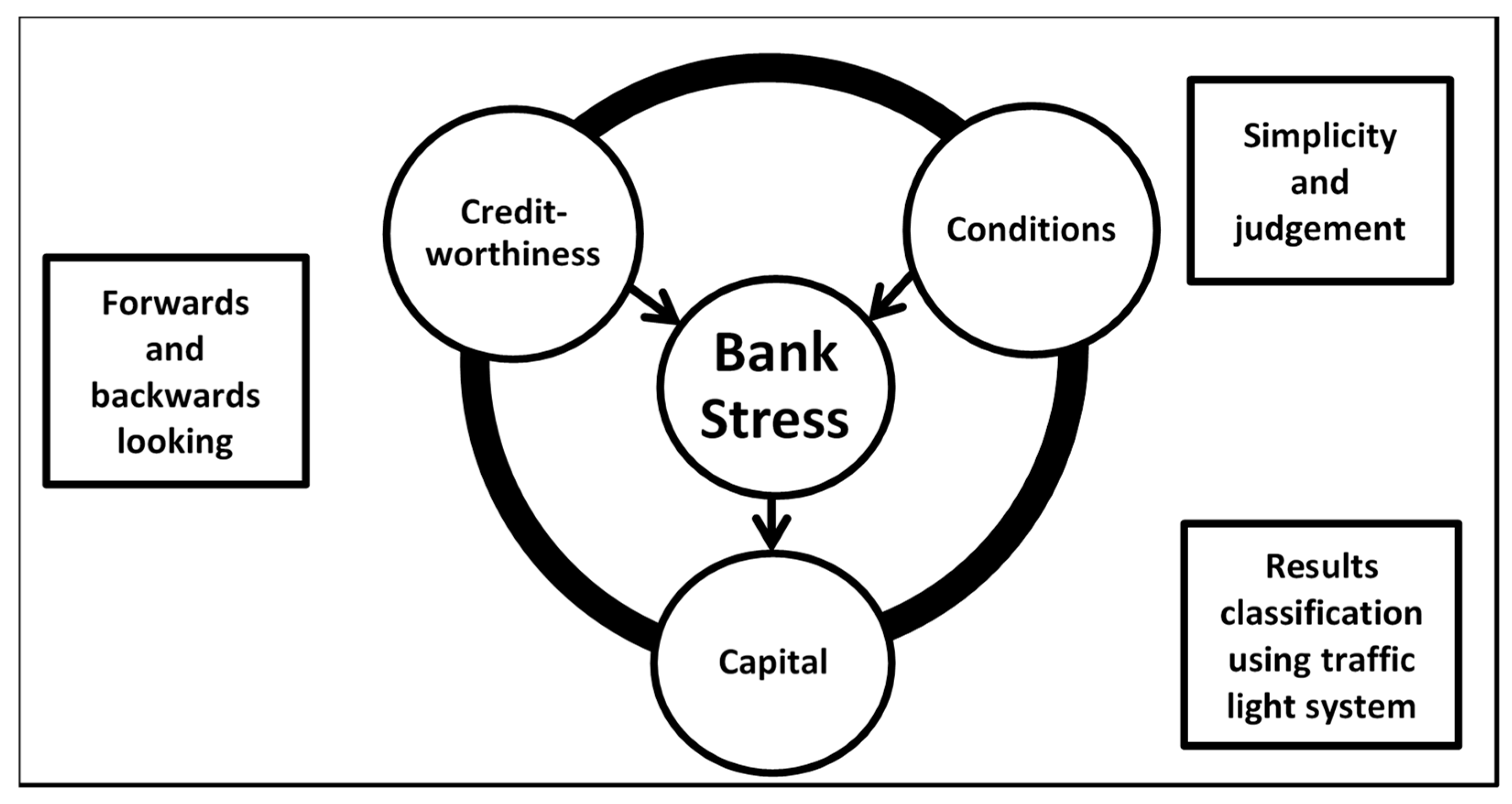
4. Model Methodology and Motivation for Factor Choice

The model, (see Figure 1), incorporates the principles outlined in Section 3 and our 3Cs of Creditworthiness, Conditions and Capital. The arrows for the causal factors of distress, Creditworthiness and Conditions, point towards bank distress. The other arrow points away from bank distress towards our distress relief factor, Capital.

Choosing the factors involved some important considerations. The key objective is a model which applies a common approach across all banks, in order to benchmark them against each other, set a standard, and indicate where improvements are needed. The model is not intended to align microscopically with each banks’ unique circumstances, nor to replace bank specific models. Thus, a complex model with detailed criteria is not sought. Rather, simplicity and uniformity are paramount in the model which is why it is restricted to the three core factors of Creditworthiness, Conditions and Capital, combined into an overall comprehensive stability indicator (CSI).

4.1. The 3C Factors

This section focuses on firstly outlining each of the three factors and the rationale for their choice, and then secondly explaining how these are combined into an overall CSI.

The objective of the components of the model is to provide core measures of internal bank specific risk (measured by Creditworthiness), external market risk impacting on banks (measured by Conditions) and the protection or safety net that banks have against risk (measured by Capital).

Creditworthiness is our internal credit risk factor, measured by NPL to total gross loans, with figures available via World Bank data at a US country level and from annual reports for individual banks. Credit risk was acknowledged as the leading source of risk for banks long before the GFC (Basel Committee on Banking Supervision 2000). This was subsequently reinforced by the role that sub-prime and securitised loans played in the GFC. (Alali and Romero 2012) and (Kim and Lee 2019) find NPLs to be very informative in the prediction of bank failure. The importance of credit risk continues to be reinforced through the major role it plays in determining capital requirements under Basel III. Credit facilities typically represent around 80% of all assets in US banks (US Federal Reserve 2018b), and around 80% of the risk weighted assets used in capital adequacy calculations of banks (as shown in their annual reports). We do not ignore the other risks, because, as we will see later, the threshold for our CSI (Equation (3) in Section 4.2) can be adjusted to incorporate the other 20% of risks like liquidity and operational risk.

Conditions is our external factor. The importance incorporating of market-based variables into stability indicators was discussed in Section 2. Our Conditions variable is the market asset value volatility of banks (measured by the (Merton 1974) structural model approach), which as, discussed in Section 2, captures all conditions impacting on an entity at the aggregate level. As the (Merton 1974) model is well documented, we only provide a brief summary of its key features here to assist the reader. Key components of the model are equity (E), volatility of equity (σ_E), market asset values of the firm (A), debt (F) and market asset value volatility (σ_A) (Conditions). The firm defaults when liabilities exceed assets. This equals the payoff of a call option on the firm’s value with strike price F. If, at time T, loans exceed assets, then the option will expire unexercised and the owners will default. The call option is in the money where A_T − F > 0, and out the money where A_T − F < 0. As A − F is a measure of the firm’s capital, in our model A = F is where the lender has run out of capital. An increase in Conditions risk indicates capital erosion, which needs to be restored, as noted by the BOE and IMF (see Section 1). In calculating the Conditions, we follow the (Merton 1974) approach, as outlined in (Bharath and Shumway 2008). An initial asset value and its volatility (σ_A) is estimated in Equation (1):

$${\sigma }_A={\sigma }_E\left(\frac{E}{E+F}\right)$$

(1)

Then a comprehensive iteration, convergence and correlation procedure is applied in order to estimate the market value of assets every day, and the standard deviation thereof, for each bank in our sample over the 13 year period. Any thin trading is compensated for using a moving average model as outlined by (Miller et al. 1994).

Capital is our safety net. Capital buffers can help reduce banks’ systemic importance and their individual risk-taking (Andries et al. 2018) and increase the resilience of banks (Hossain et al. 2017). We use a total capital to total assets ratio rather than risk-weighted regulatory ratios. Many soundness or stability indicators and their incorporation into stress tests, assess whether the existing level of regulatory capital ratios can withstand shocks. However, the accuracy of the risk-weighting process, globally, has been hotly debated given that different internal models used by banks result in different risk-weightings. The (Basel Committee on Banking Supervision 2014), attribute this problem to a mix of differences in the underlying risk and to different banking and supervisory practices. A further argument in favour of our use of an unweighted capital ratio is that the purpose of risk weighting is to apply favourable weightings to lower risk categories of loans, whereas our Creditworthiness factor is based on NPLs which all fall into the high-risk category.

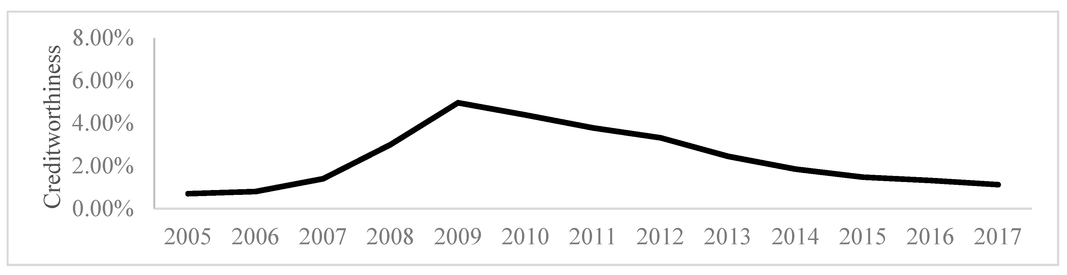
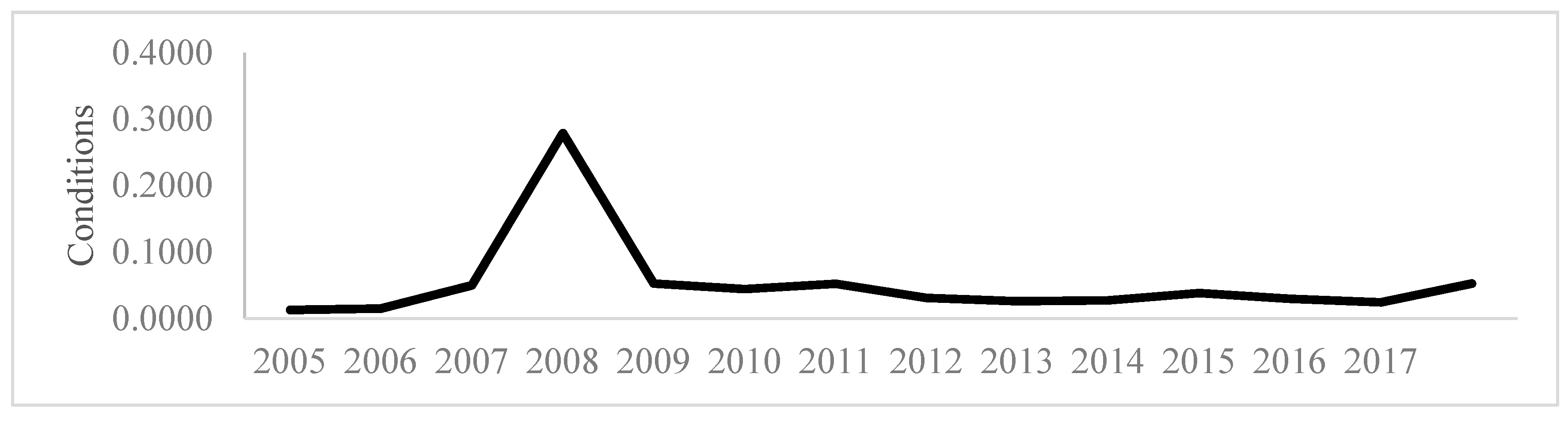
To illustrate the rationale behind the three factors chosen, consider the example of two countries (Australia and the US). Going into the GFC, the US had almost double the Leverage ratio of Australia (10.7% vs. 5.8%). Yet, the US had considerable losses and bank failures during the GFC, whereas Australian banks all remained profitable. The problem was that the US had treble the level of Creditworthiness risk (4.0% vs. 1.7%) and almost four times the Conditions risk (17.5% vs. 4.3%), leading to severe erosion of US bank market capital values, with poor ability to meet nonperforming loans. Thus, capital only tells part of the story of bank soundness. As noted by (Flannery and Giacomini 2015), many large banks’ losses were absorbed by their governments during the GFC, despite these banks complying with Basel standards for “adequate” capital. It is the deterioration of Creditworthiness and market Conditions that leads to distress and losses for banks, which causes the need for capital buffers to absorb this risk. There is not necessarily a relationship between capital and default risk (Bichsel and Blum 2007). Thus, Leverage is not a preventative measure. It is the insurance policy―the safety net in the event of a fall. It is the quality of lending and market conditions that determine distress levels. Thus, in this study we examine distress using all these factors, i.e., the 3Cs of Capital, Creditworthiness and Conditions.

4.2. The Comprehensive Stability Indicator

Once the 3Cs are calculated, our objective is to provide an overall measure of bank distress, by combining the factors into a single comprehensive stability indicator (CSI). This measures the extent to which Leverage, modified by changes in volatility in market asset values (Conditions) to derive the market value of capital KM, can cover Creditworthiness in the form of the NPL to gross loans ratio.

With the objective of ascertaining changes to CSI if distress is applied to the underlying variables, the model incorporates a distress factor (DF), which is the amount of distress applied to a particular scenario. Our zones of red, orange and green, have the objective of classifying CSI into different risk bands.

The model has the following parameters and definitions:

Conditions	= market asset value volatility, per Equation (1)
Creditworthiness	= nonperforming loans to total gross loans
Leverage	= total capital to total assets ratio
KM	= market value of capital (per Equation (2), which measures Leverage based on the impact of a change in Conditions)
CSI	= Comprehensive stability indicator (Equation (3), which is Leverage to Creditworthiness, modified by changes in Conditions)
t	= time period (year), and thus Conditionst is Conditions for historical period t
tc	= current time period (i.e., if the most recent period in the sample is 2017, then Conditionstc is Conditions2017)
DF	= distress factor, which is the predetermined shock applied to a variable in a particular scenario. In our scenario in Section 6 we apply distress to current factors up to the 90% threshold (α = 0.90) level of historical experiences (e.g., the 90th percentile worst year in our sample). Our example analysis of the US banks that is undertaken in Section 6 shows that for Conditions this is 2.0 × the current Conditions level and that the associated Creditworthiness at that distressed Conditions level is 2.5 × the current Creditworthiness level. Thus, DFConditions0.90 = 2.0 and DFCreditworthinesss0.90 = 2.5. Therefore, Conditionsdistressed = Conditionstc × 2.0 and Creditworthinessdistressed = Creditworthinesstc × 2.5.
Zone	= red, orange, or green, as determined by Section 6.1.4.
Note: The above factors are developed using figures for the total US market to determine a uniform Distress Factor (DF). This DF is then applied to the 3Cs specific to each bank in the sample.

The equations referred to above are as follows, assuming 2017 as the current year:

$$\mathit{KM}\mathrm{t}={\mathit{Leverage}}_{2017}\times ({\mathit{Conditions}}_{2017}/{\mathit{Conditions}}_{\mathrm{t}})$$

(2)

$${\mathit{CSI}}_{\mathrm{t}}={\mathit{CSI}}_{\mathrm{t}}=\frac{Leverag{e}_t}{Creditworthines{s}_t}\times \frac{Condition{s}_{2017}}{Condition{s}_t}$$

(3)

CSI serves as a financial stability indicator, measuring the extent to which Leverage, modified by changes in volatility in market asset values (Conditions), is able to cover Creditworthiness in the form of the NPL to gross loans ratio. As Creditworthiness risk increases, or as Leverage decreases, this coverage will reduce, indicating a reduction in the financial soundness of the firm. As economic and market conditions deteriorate (such as in 2008 at the height of the GFC), market asset values become more volatile, impacting on CSI. Thus, CSI₂₀₀₈ will be lower than CSI for other years in our sample, showing a deterioration in financial soundness, and a need to restore the Leverage of the firm. CSI is linked to colour bands red (danger), orange (caution) and green (pass).

5. Data and Testing the Appropriateness of the Model

This section outlines the data used in our modelling and undertakes regression testing of the appropriateness of the underlying factors of the model, prior to running and presenting the results of the full model in Section 6. Our CSI model requires data for Leverage, Creditworthiness and Conditions, including daily share price data on all individual banks in the sample. The period examined in the CSI model is from 2005 to 2017 which importantly, includes the 2008–2009 GFC period, as well as pre-GFC and post-GFC years. For Leverage and for Creditworthiness we use annual figures obtained from World Bank data at the country level, supplemented by data on individual banks obtained from Datastream and annual reports. The data we need to calculate Conditions, using the methodology outlined in Section 4 to derive the daily asset values, is also obtained from Datastream.

Because we compare our results to the sample of banks used in the Federal Reserve Stress Tests severely distressed scenario (35 banks in the 2018 tests), we only used banks in our sample which were included in those tests. Our data sample was further restricted to listed USA owned banks, in the Datastream US Banks index, and which had sufficient data available over the studied period. This gave us a sample of 20 Banks common to those from the Federal Reserve tests, including Ally, American Express, Bank of America, Bank of New York Mellon, BB&T, Capital One, Citigroup, Citizens, Discover, Fifth Third, Huntington, JP Morgan Chase, Key Corp, M&T, Morgan Stanley, Northern Trust, PNC, SunTrust, US Bancorp, and Wells Fargo. Between them, these 20 banks hold 67% of the total assets (which comprise mainly loan assets) of all US banks.

To test the appropriateness of our selected factors, we back-tested them against actual bank failures in the US, as obtained from FDIC (Federal Deposit Insurance Corporation 2017). This initial test of ours included quarterly bank failure (BF) figures for the entire US banking industry (as opposed to just our sample of 20 individual banks mentioned above), which amounted to a total of 581 failures for our studied period). Using ordinary least squares regression, we regressed these quarterly bank failure figures (BF) against quarterly aggregated figures for the entire US banking industry for Creditworthiness, Conditions, and Leverage (as defined for these three variables in Section 4.2) obtained from a combination of World Bank and DataStream data for 20 years from 1998 to 2017, thus having 80 observations for each variable.

BF = β₀ + β₁Creditworthiness_t + β₂Conditions_t + β₃Leverage_t-3 + ε

(4)

We tested a variety of lags, finding that no-lag for Creditworthiness and Leverage yielded the highest explanatory values, and for Conditions (where each quarterly observation was a rolling figure of the volatility over the prior 12 months), a lag of three quarterly periods was the most explanatory. This supported the prior findings of (Allen et al. 2015) that market factors can provide an early warning indicator of potential bank problems (in this case 9 months prior to the failure), and by the time problems actually occur, the market has moved on to new news.

The regression results are summarised in

Table 1. Summary of US banks’ test regression results.

Factor	Significance	Factor	R2	Adjusted R2
Creditworthiness	***	Creditworthiness	86.5%	86.2%
Conditions(lag3/4)	***	Creditworthiness + Conditions(lag3/4)	90.5%	90.2%
Leverage	**	All factors	91.2%	90.9%

The table shows the significance of regression variables in estimating US bank failures over a 20 year period to 2017. In the table, *** denotes significance at the 99% level and ** at the 95% level.

. R², which measures the extent to which the factors can explain BF was found to be a high 91.2% for the multiple regression, with high (99%) significance for Creditworthiness and Conditions (lag ¾ year), and relatively lower (95%) significance for Leverage. To test the additional value of each variable, we commence with our highest factor (Creditworthiness at R² = 86.5%), then add the other variables. Adding Conditions (lag ¾ year) (which on its own has an R² of 43.9%), increases the R² obtained by Creditworthiness by a further 4.0% to 90.5% but Leverage adds very little value to the explanation as seen by the very small increase in total R² of 0.7%. If we add the Credit to GDP variable recommended by Drehmann et al. in Section 2 as a good indicator of capital buffers, (which on its own has an R² of 29.5%) we improve the R² of our multiple regression model only marginally to 92.1%. These figures re-enforce Creditworthiness and Conditions as important causal factors, and Leverage as a non-causal factor, but as discussed, a safety net factor.

We found no evidence of high multicollinearity between the independent variables, which all had a low Variance Inflation Factor (VIF) of below 3. Having broadly established the significance of our underlying variables, we now undertake the full CSI modelling, with the results presented in Section 6.

6. Results of the CSI Modelling

There are two core stages in calculating and applying the CSI. The first stage (undertaken in Section 6.1) is to determine the 3Cs of the US as a whole, and to use these to calculate an annual CSI and zones (green, orange red) for the US. From this, distress factors (DF, as defined in Section 4.2), will be determined. Then (in Section 6.2), DF will be uniformly applied to the individual 3Cs of each of the 20 banks in our sample. This is to determine the individual banks’ CSIs and zones under distressed conditions, which will be compared to outcomes of Federal Reserve Dodd–Frank stress tests.

6.1. Results for the US as a Whole

This section begins by presenting summary results graphs for each of our 3C factors in Section 6.1.1, Section 6.1.2 and Section 6.1.3. Then Section 6.1.4 presents the CSI modelling results for the US.

6.1.1. Factor 1: Creditworthiness

While the US Creditworthiness₂₀₁₇ risk is at relatively low historical levels (Figure 2), the US had low Creditworthiness risk (below 1%) just prior to the GFC, which spiked during the GFC (almost 5%), after which, financial sector reforms such as the Dodd–Frank Act were introduced, and Creditworthiness showed a reducing trend to 1.13% in 2017. The lines in Figure 2 plot the annual figure for Creditworthiness, which as defined in Section 4 is NPL to Gross Loans for U.S. banks as provided by the World Bank at an aggregated country level.

6.1.2. Factor 2: Conditions

Our market-based metric is Conditions, measured by market asset value volatility. The US demonstrated a huge spike in the GFC as seen in Figure 3, where the lines in Figure 3 plot the annual Conditions.

6.1.3. Factor 3: Capital

The lines in Figure 4a plot annual Leverage, which, as defined in Section 4, is total capital to total assets ratio for banks, as provided by the World Bank at the country level. The lines in Figure 4b plot the annual market value of capital KM, which is defined in Section 4 and measured by Equation (2). As seen in Figure 4a, Leverage, which is based on book values, has stayed far more consistent than the market values of capital, which showed a large drop to almost zero during the GFC, thereafter showing an upward trend (though still volatile compared to Leverage).

6.1.4. Combined Factors: The Comprehensive Stability Indicator (CSI)

In

Table 2. Historical figures for the US banking market as a whole.

Year (t)	Creditworthiness	β	Leverage	Β	Conditions	β	KM	β	CSI	Zone
2005	0.70%	0.25	10.30%	0.88	0.013	0.21	21.96%	2.83	31.37	Green
2006	0.80%	0.29	10.50%	0.90	0.015	0.25	19.03%	2.45	23.79	Green
2007	1.40%	0.51	10.30%	0.88	0.050	0.83	5.71%	0.74	4.08	Green
2008	3.00%	1.08	9.30%	0.79	0.279	4.61	1.02%	0.13	0.34	Red
2009	4.96%	1.79	12.37%	1.06	0.052	0.87	5.41%	0.70	1.09	Red
2010	4.39%	1.59	12.74%	1.09	0.044	0.73	6.43%	0.83	1.47	Orange
2011	3.78%	1.37	12.23%	1.05	0.052	0.86	5.46%	0.70	1.44	Orange
2012	3.32%	1.20	11.96%	1.02	0.031	0.51	9.17%	1.18	2.76	Green
2013	2.45%	0.89	11.78%	1.01	0.026	0.43	11.00%	1.42	4.49	Green
2014	1.85%	0.67	11.66%	1.00	0.027	0.45	10.47%	1.35	5.66	Green
2015	1.47%	0.53	11.71%	1.00	0.039	0.64	7.40%	0.95	5.02	Green
2016	1.32%	0.48	11.59%	0.99	0.030	0.49	9.57%	1.23	7.25	Green
2017	1.13%	0.41	11.65%	1.00	0.024	0.40	11.65%	1.50	10.34	Green
Average	2.35%		11.39%		0.052		9.56%		7.62
90th percentile					0.052

Notes: Leverage is total capital to total assets ratio. Conditions is market value asset volatility, calculated as shown in Section 4. KM (market value of capital) is per Equation (2), where KM = Leverage x (Conditions₂₀₁₇/Conditions_t) and CSI (comprehensive stability indicator) is per Equation (3), where CSI_t = KM_t/Creditworthiness_t, and t represents the year for which the statistic is being calculated. Zones have been set according to the CSI level as: red < 1.2, orange < 2, green ≥ 2. β (Beta)is the relevant statistic for year t as shown in the prior column, relative to the long-term average for that variable (as shown in the final row of that column). The 90th percentile (α = 0.90) is the 90th percentile ranking for an indicator (e.g., 9th best or second worst in a 10 year sample, which lies slightly below the 12th ranked observation in a 13 year sample).

, we show historical zones (red, orange, green) and CSI calculations for each year.

A summary of the calculation methods is included in the notes to the table. While there are many possible alternative methods of setting thresholds for various purposes, (see for example (Hansen 2000)), for the purposes of illustrating our model, CSI thresholds for the colour zones were set as follows: red < 1.2, orange < 2, green ≥ 2. These zones can be set by the bank or regulator according to their requirements or risk tolerance. The threshold we set here between orange and red is not arbitrary—having a CSI ratio of 1.2 or above (i.e., above red) means that Creditworthiness is fully covered by KM with a 20% buffer to cover other risks such as Market and Operational risk (which we have already noted form around 20% of the risks of US Banks). The model not only highlights pass/fail but identifies banks where improvements could be made (orange).

6.2. Results for Individual Banks Compared to Federal Reserve Tests

We compared outcomes from our model to the US Federal Reserve (2018a, 2015) Dodd–Frank stress tests for the 20 banks in our sample. The 2018 Federal Reserve tests were undertaken on 2017 US Banks’ data and the 2015 Federal Reserve tests on 2014 data. We began by calculating DF factors from the 2017 figures in the above table, applying them to the 20 US banks in the sample, and comparing these outcomes to results for the same banks from the 2018 Federal Reserve tests. We found that all 20 banks achieved green on our model. This was a similar result to the 2018 US Federal Reserve tests, where all banks were found to have passed due to being above the required regulatory capital ratios based on the severely distressed scenario. This is not surprising, given the vastly improved Creditworthiness, Conditions, KM and CSI figures for the US over the past few years that we have shown in this study. However, when we went back to the 2015 Federal Reserve tests (based on 2014 data), a greater range of pass/caution/fail results were provided by the CSI model (based on 2014 3Cs data), which better illustrates the nuances of our model than the 2018 tests. Hence the detailed comparisons to the 2015 tests (based on 2014 data) are the ones we present here.

Table 2 was based on historical zones (looking back) for the US market as a whole. We then ascertained, based on the individual Leverage₂₀₁₄ and Creditworthiness₂₀₁₄ for each of the 20 banks in the sample, how well each individual bank could withstand a future shock that reflects realistic and plausible extreme changes to Conditions, guided by the past volatility of the US market. The distressed scenario thus applied a uniform shock to each of the banks in the sample, and ascertained changes to their colour zone. For the overall US banking market, calculated from figures in Table 2, Conditions_0.90 was approximately 2.0× higher than Conditions₂₀₁₄ and Creditworthiness at the Conditions_0.90 level exceeded Creditworthiness₂₀₁₄ by approximately 2.5×. So, to illustrate our model, we used these as our distress factors (DF_Conditions = 2.0; DF_{Creditworthiness} = 2.5) to apply to the 20 individual banks. Thus, Conditions_distressed = Conditions₂₀₁₄ × 2.0, and Creditworthiness_distressed = Creditworthiness₂₀₁₄ × 2.5. Again, banks or regulators can determine their own distress factors. We then used these Creditworthiness_distressed and Conditions_distressed values to calculate KM_distressed (=Leverage₂₀₁₄ × Conditions₂₀₁₄/Conditions_distressed), CSI_distressed, (=KM_distressed/Creditworthiness_distressed) and Zone_distressed for each bank. As shown in

Table 3. Summary statistics for 20 US banks.

Zone (Our Model)	Count	%	Association b/w Our Model and Fed Tier 1 Model
Green	15	75.0%	n	20
Orange	5	25.0%	r	0.662
Red	0	0.0%	t	3.751
			Critical value 95%	2.101
			Critical value 99%	2.878
			Significance	***

The table applies our CSI zones to 20 US banks, and then compares the ranking of the banks on our model to the ranking of US Federal Reserve stress tests. n is number of observations, r is the Spearman rank correlation coefficient, and t measures the significance of r using a t test and must exceed the critical value to be significant. *** Denotes significance at the 99% level.

, applying these factors to our model achieved a 99% level of confidence similarity to the Federal Reserve tests in the rankings of banks (best to worst), using a Spearman ranking correlation test which compares the relative ordinal risk of observations across datasets (Powell et al. 2018).

A key difference is that, whereas the Federal Reserve results issued every bank with a pass based on a pass/fail grading, our traffic light system, with its additional ‘caution’ (orange) category, classified 25% of banks (five banks) as orange. As shown in Table 2, the overall US banking system, while showing an overall green on our model in 2014, nonetheless has much higher Creditworthiness and overall CSI risk than is shown in 2017, and it is therefore not surprising that some banks achieved orange in our tests based on the 2014 data. A quartile analysis of the results in

Table 4. Quartile statistics for 20 US banks (five banks per quartile).

Quartile	Fed Model—Stressed Tier 1 Ratio (%)	Our Model—Distressed CSI
Q1 average	12.7	5.0
Q2 average	10.1	3.4
Q3 average	9.1	3.1
Q4 average	7.3	1.8
Quartile		No. Green	% Green	No Orange	% Orange
Q1–3 (15 banks)		14	93.3%	1	6.7%
Q4 (five banks)		1	20.0%	4	80.0%

The table compares outcomes of US Federal Reserve Stress Tests (Stressed Tier 1%) for five banks per quartile (where Q1 is lowest risk), to those same banks using our distressed CSI test. The lower half of the table shows the zones achieved for those banks on the distressed CSI test.

provides a very interesting comparison.

The 20 banks in our sample were allocated to these quartiles according to their ranking for the severely stressed tier 1 ratio achieved in the 2015 Federal Reserve Bank Dodd–Frank stress tests. Q1 is the least risky quartile (the average of those five banks with the highest tier 1 ratios), and Q4 is the riskiest quartile. The first results column in the upper section of Table 4 shows the average stressed Tier 1 ratio for each quartile, compared to the second results column which shows average distressed coverage (CSI²⁰¹⁴ per Equation (3)) for our model, for the same set of banks as contained in column 1 for each quartile. What is evident is that, as the risk increases for each quartile on the US Federal Reserve tests, our model also shows a corresponding increase in risk. The lower section of Table 4 shows the percentage of banks that achieved orange on our model out of the 15 banks in the lower risk quartiles Q1–3, as compared to the highest risk Q4 quartiles. 80% of our oranges align with the banks in the highest risk quartile of U.S. Federal Reserve tests. Overall, therefore, our model ranks banks very similar (at a 99% confidence level per Table 3) to the U.S. Federal reserve tests, but it has the advantage of the orange ‘warning’ indicator.

7. Conclusions and Implications

Stability indicators are essential to understand the ability of banks to withstand adverse financial and economic shocks. This paper developed a CSI model which uses three single factors (3Cs), Creditworthiness, Conditions and Capital to capture the risk of banks. The 3Cs were shown to be strong determinants of bank failures and the CSI model demonstrated the capacity to achieve significantly similar risk ranking of banks to the much more complex Federal Reserve tests, with the added benefit of the traffic light system which highlighted banks that needed improvement (orange). While our model is based around specific parameters for assessing bank safety, we also highlighted the importance of exercising sound judgment in interpreting results and implementing remedial measures.

The CSI model has implications for both banks and regulators. It is usually only practical to undertake formal stress tests, with a high number of variables and scenarios, on a periodic basis and not all banks have sufficient modelling capacity to undertake the highly detailed and sophisticated modelling required. The simplicity of the CSI model in using only three factors, however, means that it can be readily used to measure risk between formal stress tests, or applied by banks and regulators to banks which are not included in the formal stress tests, or to compare financial distress across multiple entities or potentially across countries. This can help increase the frequency and coverage of the measurement of bank risk. The use of the CSI, coupled with the warning indicator (orange), can allow regulators and banks to identify risk at an early stage and implement contingency plans to address the risk, thus helping to avoid more serious circumstances such as the bankruptcy of individual banks or systemic financial crises.

In terms of potential future studies, the model could be applied to developing regions, who might not have the depth of data and systems required to undertake highly detailed and complex stress testing, but who could benefit from the application of the relatively simpler 3Cs-based CSI.