A New Heavy Tailed Class of Distributions Which Includes the Pareto

Abstract

In this paper, a new heavy-tailed distribution, the mixture Pareto-loggamma distribution, derived through an exponential transformation of the generalized Lindley distribution is introduced. The resulting model is expressed as a convex sum of the classical Pareto and a special case of the loggamma distribution. A comprehensive exploration of its statistical properties and theoretical results related to insurance are provided. Estimation is performed by using the method of log-moments and maximum likelihood. Also, as the modal value of this distribution is expressed in closed-form, composite parametric models are easily obtained by a mode matching procedure. The performance of both the mixture Pareto-loggamma distribution and composite models are tested by employing different claims datasets.

1. Introduction

In general insurance, pricing is one of the most complex processes and is no easy task but a long-drawn exercise involving the crucial step of modeling past claim data. For modeling insurance claims data, finding a suitable distribution to unearth the information from the data is a crucial work to help the practitioners to calculate fair premiums. In actuarial statistics and finance, the classical Pareto distribution has been deemed better than other models because it provides a good description of the random behaviour of large claims. Loss data mostly have several characteristics such as unimodality, right skewness, and a thick right tail. To accommodate these features in a single model, many probability models have been proposed in the literature.

Over the last decades, different approaches to derive new classes of probability distributions that could provide more flexibility when modelling large losses has been added to the literature. This includes transformation method, the composition of two or more distributions, compounding of distributions or a finite mixture of distributions among other methodologies. In particular for generalizations of the classical Pareto distribution, the reader is referred to the Stoppa distribution (see Stoppa 1990), the Pareto positive stable distribution (see Sarabia and Prieto 2009), the Pareto ArcTan distribution (see Gómez-Déniz and Calderín-Ojeda 2015) and the generalized Pareto distribution proposed in Ghitany et al. (2018). Obviously, adding a parameter to the parent model complicates the parameter estimation.

In this paper, a probabilistic family, the mixture Pareto-loggamma distribution, which belongs to the heavy-tailed class of probabilistic models is introduced. This family is derived by using of an exponential transformation of the generalized Lindley distribution. It is expressed as a convex sum of the classical Pareto and a special case of the loggamma distribution similar to the one presented in Gómez-Déniz and Calderín-Ojeda (2014). The former model is obtained as a particular case whereas the latter one is a limiting case. We further present expressions of statistical and actuarial measures such as moments, variance, cumulative distribution function, hazard rate function, VaR, TVaR and limited expected values. For many of these distributional characteristics, closed-form expressions are obtained. Estimation of the parameters of this distribution can be easily calculated by the maximum likelihood method by using the numerical search of the maximum and also by the method of log-moments.

In many instances, composite distributions give a reasonably good fit as compared to classical distributions since the former models have the advantage of accommodating both low magnitude values with a high frequency as well as large magnitude figures with low frequency. Cooray and Ananda (2005) introduced a composite lognormal-Pareto distribution with restricted mixing weights. Scollnik (2007) improved the composite lognormal-Pareto model by allowing flexible mixing weights. Bakar et al. (2015) considered several probabilistic models in place of lognormal and Pareto distribution using the approach discussed in Scollnik (2007). Recently, Calderín-Ojeda and Kwok (2016) introduced a new class of composite model using mode-matching procedure. They derived composite models using lognormal and Weibull distributions with a Stoppa model, a generalization of the Pareto distribution. As there exists a closed-form expression for the modal value of this new model, in this article, we use the mode-matching procedure to derive new composite models based on this distribution.

The structure of the paper is organized as follows. In Section 2, we present the genesis of the new distribution, and discuss its relationship with other distributions. Besides, the most relevant distributional properties are studied in the same section. Also, different estimation methods are examined. Finally, composite models based on the proposed distribution are derived. Next, in Section 3, some results related to insurance are displayed. Numerical applications are displayed in Section 4 together with the derivation of some income indices. The last section concludes the paper.

2. The $\mathcal{MPLG}$ Distribution and Its Properties

It can be easily seen that the following expression

$$f_X\left(x\right|\theta ,\lambda ,x_0)=\frac{{\theta }^2}{x(\theta +\lambda )}{\left(\frac{x}{x_0}\right)}^{-\theta }\left(1+\lambda log\left(\frac{x}{x_0}\right)\right)x\ge x_0>0$$

(1)

with $\lambda \ge 0$ and $\theta >0$ is a genuine probability density function (pdf). Here $\theta ,\lambda$ are shape parameter and $x_0$ is scale parameter (see the Appendix A). Note that the pdf (1) can be written as a convex sum of the classical Pareto distribution and a special case of the loggamma distribution. The former model is obtained when $\lambda =0$ and the latter one for $\lambda \to \infty$. Observe that the pdf of the loggamma distribution considered in this work is

$$f_X\left(x\right|\theta ,\gamma ,x_0)=\frac{{\theta }^{\gamma }}{x_0\mathsf{\Gamma }\left(\gamma \right)}{\left(\frac{x}{x_0}\right)}^{-(\theta +1)}log{\left(\frac{x}{x_0}\right)}^{\gamma -1},$$

with $\theta ,\gamma >0$ and $x\ge x_0$. In our model it is assumed that $\gamma =2$.

The cumulative distribution function (cdf), survival function (sf) and hazard rate function of a random variable (rv) with pdf (1) are respectively given, for $x\ge x_0$, as

$$F_X\left(x\right)=1-\frac{\left(\theta +\lambda +\theta \lambda log\left(\frac{x}{x_0}\right)\right)}{\theta +\lambda }{\left(\frac{x}{x_0}\right)}^{-\theta },$$

(2)

$${\overline{F}}_X\left(x\right)=\frac{\left(\theta +\lambda +\theta \lambda log\left(\frac{x}{x_0}\right)\right)}{\theta +\lambda }{\left(\frac{x}{x_0}\right)}^{-\theta },$$

(3)

$$h_X\left(x\right)=\frac{\theta }{x}\left(1-\frac{\lambda }{\theta +\lambda +\theta \lambda log\left(\frac{x}{x_0}\right)}\right).$$

(4)

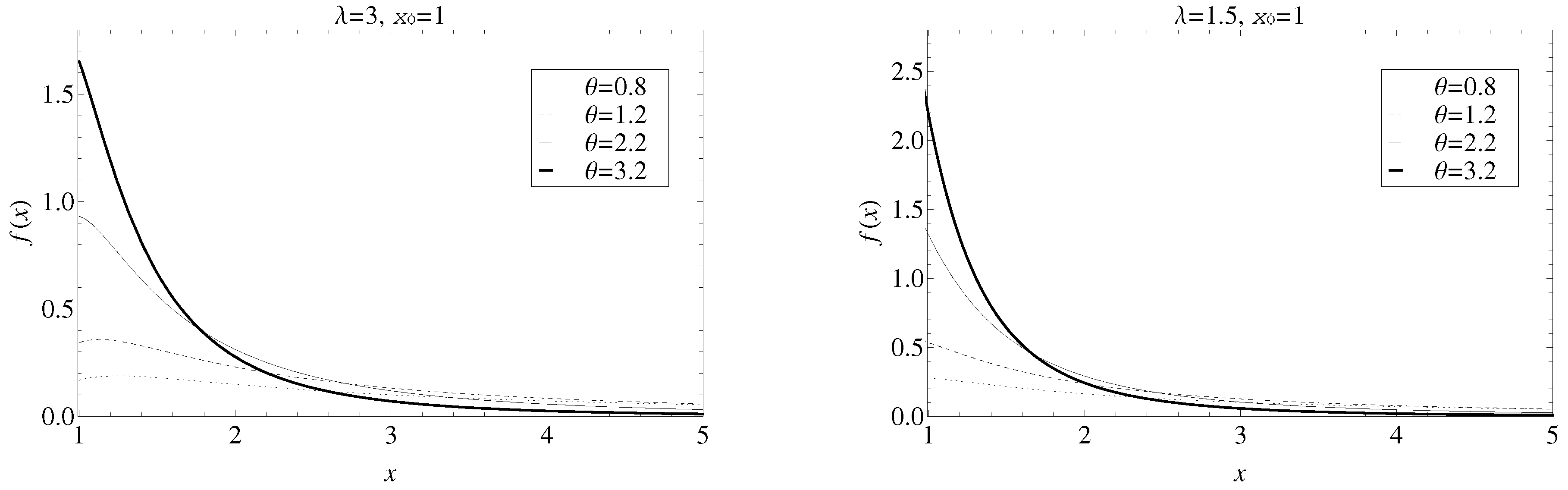
Henceforth, a continuous rv X that follows (1) will be called as mixture Pareto-loggamma distribution and denoted as $\mathcal{MPLG}(\theta ,\lambda ,x_0)$. The shape of the pdf given in (1) is shown in Figure 1 for different values of the parameters $\theta$ and $\lambda$ and a fixed $x_0$. It is observable that the larger is the value of $\theta$, the thinner is the tail. On the contrary, the thickness of the tail decreases when $\lambda$ drops.

Undoubtedly, the single parameter Pareto distribution is one of the most attractive distributions in statistics; a power-law probability distribution found in a large number of real-world situations inside and outside the field of economics. Furthermore, it is usually used as a basis for Excess of Loss quotations as it gives a pretty good description of the random behavior of large losses. In this sense, many probability distributions can be used for modelling single loss amounts. Then, if the loss is assumed to follow the pdf (1), we have that $\theta$ defines the tail behavior of the distribution.

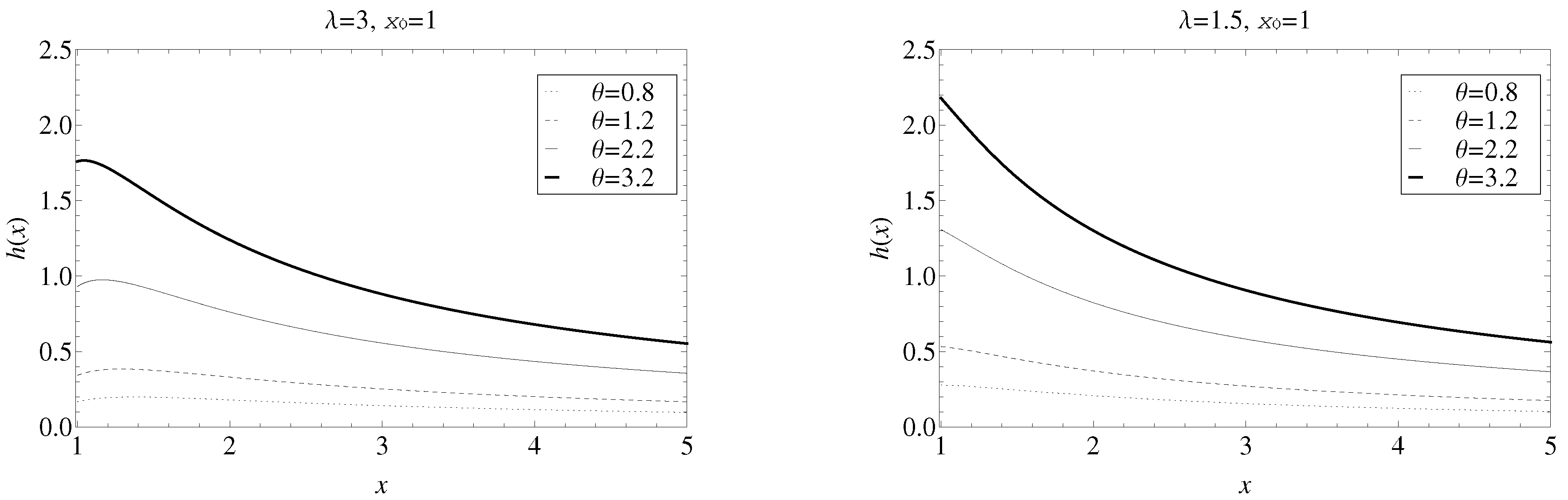
Below, the hazard rate function has been plotted in Figure 2 for different values of the parameters $\theta$ and $\lambda$ for fixed $x_0$. It is observable that the hazard rate function increases when the parameter $\theta$ grows and the parameter $\lambda$ declines.

The next result shows the relationship between the $\mathcal{MPLG}$ and the Generalized Lindley distribution, which is extensively used in lifetime analysis and reliability.

Remark 1.

The$\mathcal{MPLG}(\theta ,\lambda ,x_0)$distribution can be also obtained by taking$X=x_{0}exp\left\{Y\right\}$, where Y follows a generalized Lindley distribution with density

$$g_Y\left(y\right)=\frac{{\theta }^2}{(\theta +\lambda )}(1+\lambda y)exp\{-\theta y\},y>0,\lambda ,\theta >0.$$

(5)

From this result, it is straightforward to generate random variates from the $\mathcal{MPLG}(\theta ,\lambda ,x_0)$ distribution by observing that the pdf given in (5), can be rewritten as

$$w\left(y\right)=p{a}_1\left(y\right)+(1-p)a_2\left(y\right),$$

where ${\displaystyle p=\frac{\theta }{\theta +\lambda }}$, $a_1(·)$ is the pdf of the exponential distribution with mean $1/\theta$ and $a_2(·)$ is the pdf of the Erlang distribution with shape parameter 2 and rate parameter $\theta$. Then, a random variate from the $\mathcal{MPLG}$ distribution, x, can be generated following a modification of the algorithm presented in Ghitany et al. (2008) as shown below.

• Generate two random numbers $u_1$ and $u_2$ from the standard uniform distribution, $U(0,1)$.
• Generate random variates ${\tilde{a}}_1$ from the exponential distribution with mean $1/\theta$ and ${\tilde{a}}_2$ from the Erlang distribution with shape parameter 2 and rate parameter $\theta$ by using $u_1$.
• If $u_2\le p$, then set $y={\tilde{a}}_1$; otherwise, set $y={\tilde{a}}_2$.
• Generate $x=x_{0}exp\left\{y\right\}$.

Observe that an analogous algorithm could be implemented by using the fact that (1) is a convex sum of the densities of Pareto and loggamma distributions.

2.1. Moments and Log-Moments

The rth raw moment of $\mathcal{MPLG}(\theta ,\lambda ,x_0)$ is given by

$$\mathbb{E}\left(X^r\right)=\frac{{\theta }^2{x}_0^r(\theta +\lambda -r)}{(\theta +\lambda ){(r-\theta )}^2}\theta \ne r.$$

In particular, we have that

$$\begin{array}{cc}\hfill \mu =\mathbb{E}\left(X\right)& =\frac{{\theta }^2{x}_o(\theta +\lambda -1)}{{(\theta -1)}^2(\theta +\lambda )},\theta \ne 1\mathrm{and}\hfill \\ \hfill \mathbb{E}\left(X^2\right)& =\frac{{\theta }^2{x}_0^2(\theta +\lambda -2)}{(\theta +\lambda ){(2-\theta )}^2},\theta \ne 2.\hfill \end{array}$$

The variance is given by

$$\mathbb{V}\left(X\right)=\frac{{\theta }^2{x}_0^2(\theta +\lambda -2)}{(\theta +\lambda ){(2-\theta )}^2}-{\left(\frac{{\theta }^2{x}_0(\theta +\lambda -1)}{(\theta +\lambda ){(1-\theta )}^2}\right)}^2,\theta \ne 1,2.$$

(6)

Remark 1 can be used to obtain the rth raw log-moment of the density (1)

$$l_s=\mathbb{E}{\left(log\left(\frac{X}{x_0}\right)\right)}^s=\frac{s!(\theta +\lambda +\lambda s)}{{\theta }^s(\theta +\lambda )}.$$

(7)

The moment estimator of $\theta$ and $\lambda$ with known $x_0$ can be simply derived from (7).

2.2. Unimodality

The modal value of the $\mathcal{MPLG}$ distribution can be found by taking the first derivative of the pdf (1),

$$f^{\prime }\left(x\right)=\frac{{\theta }^2{x}_0^{\theta }{x}^{-\theta -2}}{\theta +\lambda }\left(\lambda -(1+\theta )\left(1+\lambda log\left(\frac{x}{x_0}\right)\right)\right),$$

(8)

then, by setting (8) equal to zero and solving for x, the mode is $x_m=x_{0}exp\left\{\frac{\lambda -\theta -1}{\lambda (\theta +1)}\right\}$. If $\lambda \le \theta +1$, then the mode is at $x_m=x_0$.

2.3. Stochastic Ordering

Many parametric families of distributions can be ordered by some stochastic orders according to the value of their parameters. A rv $X_1$ is said to be stochastically smaller $\left(X_1{\le }_{st}{X}_2\right)$ than $X_2$ if $F_{X_1}\left(x\right)\ge F_{X_2}\left(x\right)$ for all x. The formal definition of stochastic ordering is

Definition 1.

Let$X_1$and$X_2$be continuous random variables with densities$f_1$and$f_2$, respectively, such that$\frac{f_2\left(x\right)}{f_1\left(x\right)}$is non-decreasing over the union of the supports of$X_1$and$X_2$. Then$X_1$is said to be smaller than$X_2$in the likelihood ratio order.$\left(X_1{\le }_{lr}{X}_2\right)$(see Section 1.C of Shaked and Shanthikumar (2007)).

Similarly, a rv can be also ordered for stochastic (distribution function), hazard rate and mean excess orders when the following results hold:

(i)

Stochastic order $\left(X_1{\le }_{st}{X}_2\right)$ if $F_{X_1}\left(x\right)\ge F_{X_2}\left(x\right)$ for all x.

(ii)

Hazard rate order $\left(X_1{\le }_{hr}{X}_2\right)$ if $h_{X_1}\left(x\right)\ge h_{X_2}\left(x\right)$ for all x.

(iii)

Mean excess order $\left(X_1{\le }_{me}{X}_2\right)$ if $e_{X_1}\left(x\right)\ge e_{X_2}\left(x\right)$ for all x, where $e_X(·)$ is mean excess function given in expression (17).

Using Theorem 1.C.1 and Theorem 2.A.1 of Shaked and Shanthikumar (2007), the above stochastic orders hold following implications result

$$\begin{array}{cc}\hfill \left(X_1{\le }_{lr}{X}_2\right)\Rightarrow (X_1& {\le }_{hr}{X}_2)\Rightarrow \left(X_1{\le }_{me}{X}_2\right)\hfill \\ \hfill & \Downarrow \hfill \\ \hfill (X_1& {\le }_{st}{X}_2).\hfill \end{array}$$

(9)

This gives rise to Proposition 1.

Proposition 1.

Let$X_1$and$X_2$be two rv’s having$\mathcal{MPLG}$distribution with parameters$({\theta }_i,{\lambda }_i,x_{0i})$$i=1,2$. Then following results hold

i. 

If$x_{01}=x_{02}$,${\theta }_1\ge {\theta }_2$and${\lambda }_1\le {\lambda }_2$, then$X_1{\le }_{lr}{X}_2$,$X_1{\le }_{hr}{X}_2$and$X_1{\le }_{st}{X}_2$.

ii. 

If$x_{01}\le x_{02}$,${\theta }_1={\theta }_2$and${\lambda }_1={\lambda }_2$, then$X_1{\le }_{lr}{X}_2$,$X_1{\le }_{hr}{X}_2$and$X_1{\le }_{st}{X}_2$.

Proof. 

See the Appendix A. □

2.4. Integrated Tail Distribution and Equilibrium Hazard Rate

As we have already seen previously, the proposed distribution can be viewed as a mixture of two thick-tailed distributions, the Pareto and loggamma models, thus it can be used to describe events that include heavy-tailed behaviour. In this particular, we define another distribution function called Integrated tail distribution (ITD) (also known as equilibrium distribution) $F_e\left(x\right)$ which often appears in insurance fields (see Yang 2004). The ITD has many interesting applications, e.g., approximation of the ruin function (see Yang 2004) or characterisation of the tail of the distribution (see Su and Tang 2003) just to name a few. Hence, for $\mathcal{MPLG}(\theta ,\lambda ,x_0)$ distribution bluewith $\theta >1$, ITD is obtained as

$$\begin{array}{ccc}\hfill F_e\left(x\right)& =& {\displaystyle \frac{1}{\mathbb{E}\left(X\right)}{\int }_{x_0}^x\overline{F}\left(y\right)dy}\hfill \\ & \hfill =& \frac{{(\theta -1)}^2(\theta +\lambda )}{{\theta }^2{x}_0(\theta +\lambda -1)}\left(\frac{\theta \lambda \left(x_0-x{\left(\frac{x}{x_0}\right)}^{-\theta }\left(1-(1-\theta )log\left(\frac{x}{x_0}\right)\right)\right)}{{(1-\theta )}^2(\theta +\lambda )}+\frac{x{\left(\frac{x}{x_0}\right)}^{-\theta }-x_0}{1-\theta }\right)\hfill \\ & \hfill =& \frac{{\left(\frac{x}{x_0}\right)}^{-\theta }\left((\theta (1-\theta -2\lambda )+\lambda )\left(x-x_0{\left(\frac{x}{x_0}\right)}^{\theta }\right)+(1+\theta )\theta \lambda xlog\left(\frac{x}{x_0}\right)\right)}{{\theta }^2{x}_0(\theta +\lambda -1)}.\hfill \end{array}$$

(10)

The associated equilibrium hazard rate $r_e\left(x\right)={\left(-log\left(1-F_e\left(x\right)\right)\right)}^{\prime }$, for $\theta >1$ is given by

$$r_e\left(x\right)=\frac{{(\theta -1)}^2\left(\theta +\lambda +\theta \lambda log\left(\frac{x}{x_0}\right)\right)}{x\left(\theta (\theta +2\lambda -1)-\lambda +(\theta -1)\theta \lambda log\left(\frac{x}{x_0}\right)\right)}.$$

(11)

Moreover, it can be easily verified that ${\displaystyle \underset{x\to \infty }{lim}{r}_e\left(x\right)=0}$. Hence by using Theorem 2.1 of Su and Tang (2003) we can conclude that $\mathcal{MPLG}(\theta ,\lambda ,x_0)$ is a heavy-tailed distribution. Heavy-tailed distributions are important in non-life insurance when modeling losses related to motor third-party liability insurance, fire insurance or catastrophe insurance.

2.5. Estimation

Let $x_1,\dots ,x_n$ be an independent and identically distributed (iid) random sample of size n drawn from a population which follows a $\mathcal{MPLG}(\theta ,\lambda ,x_0)$ distribution. Estimate of parameter $x_0$ can easily be obtained, as the support of the $\mathcal{MPLG}(\theta ,\lambda ,x_0)$ distribution is greater than ${\widehat{x}}_0=min(x_1,\dots ,x_n)$. Therefore for $x_0$ known, we estimate the parameters $\theta$ and $\lambda$ by (i) method of log-moments and (ii) maximum likelihood method.

2.5.1. Method of Log-Moments

The first and second log-moments of $\mathcal{MPLG}(\theta ,\lambda ,x_0)$ distribution obtained by using (7) are given by ${\displaystyle l_1=\frac{(\theta +2\lambda )}{\theta (\theta +\lambda )}}$ and ${\displaystyle l_2=\frac{2(\theta +3\lambda )}{{\theta }^2(\theta +\lambda )}}$. Solving these equations for $\theta$ and $\lambda$, we have that these estimates are provided by

$$\tilde{\theta }=\frac{\sqrt{l_1^2-l_2}+l_1}{l_2}\mathrm{and}\tilde{\lambda }=\frac{3l_1{l}_2-3l_1^3-3l_1^2\sqrt{l_1^2-l_2}+2l_2\sqrt{l_1^2-l_2}}{l_2(3l_1^2-4l_2)}.$$

2.5.2. Maximum Likelihood Estimation

The log-likelihood function given the iid random sample $\underline{x}:=x_1,\dots ,x_n$ of size n is

$$\begin{array}{ccc}\hfill {\ell }_n(\theta ,\lambda |\underline{x})& =& 2nlog\theta -nlog(\theta +\lambda )+\sum _{i=1}^{n}log\left(1+\lambda log\left(\frac{x_i}{x_0}\right)\right)\hfill \\ & -& \theta \sum _{i=1}^{n}log\left(\frac{x_i}{x_0}\right)-\sum _{i=1}^{n}log{x}_i,\hfill \end{array}$$

(12)

and the normal equations obtained by differentiating (12) with respect to $\theta$ and $\lambda$ are

$$\frac{\partial {\ell }_n(\theta ,\lambda |\underline{x})}{\partial \theta }=\frac{2n}{\theta }-\frac{n}{\theta +\lambda }-\sum _{i=1}^{n}log\left(\frac{x_i}{x_0}\right),\frac{\partial {\ell }_n(\theta ,\lambda |\underline{x})}{\partial \lambda }=-\frac{n}{\theta +\lambda }-\sum _{i=1}^n\frac{log\left(\frac{x_i}{x_0}\right)}{1+\lambda log\left(\frac{x_i}{x_0}\right)}.$$

The above equations cannot be solved analytically and hence maximum likelihood estimates of $\theta$ and $\lambda$ can be computed numerically using in-built $\mathtt{R}$-function such as $\mathtt{nlm}\mathtt{\left(}\mathtt{\right)}$, $\mathtt{maxlik}\mathtt{\left(}\mathtt{\right)}$ or $\mathtt{optim}\mathtt{\left(}\mathtt{\right)}$. Moreover, in all these functions to initialize the program we use initial values obtained from the method of log-moments. The second partial derivative of log-likelihood function with respect to parameter $\theta$ and $\lambda$ are

$$\begin{array}{cc}\hfill \frac{{\partial }^2{\ell }_n(\theta ,\lambda |\underline{x})}{\partial {\theta }^2}=& -\frac{2n}{{\theta }^2}+\frac{n}{{(\theta +\lambda )}^2},\frac{{\partial }^2{\ell }_n(\theta ,\lambda |\underline{x})}{\partial \theta \partial \lambda }=\frac{n}{{(\theta +\lambda )}^2},\hfill \\ \hfill \frac{{\partial }^2{\ell }_n(\theta ,\lambda |\underline{x})}{\partial {\lambda }^2}=& \frac{n}{{(\theta +\lambda )}^2}-\sum _{i=1}^n\frac{{log}^2\left(\frac{x_i}{x_0}\right)}{{\left(1+\lambda log\left(\frac{x_i}{x_0}\right)\right)}^2}.\hfill \end{array}$$

(13)

Furthermore,

$${\displaystyle \mathbb{E}\left(\frac{{log}^2\left(\frac{X}{x_0}\right)}{{\left(1+\lambda log\left(\frac{X}{x_0}\right)\right)}^2}\right)=\frac{{\theta }^2}{(\theta +\lambda )}{\int }_{x_0}^{\infty }\frac{{log}^2\left(\frac{x}{x_0}\right)}{{\left(1+\lambda log\left(\frac{x}{x_0}\right)\right)}^2}{\left(\frac{x}{x_0}\right)}^{-\theta }\frac{1}{x}\left(1+\lambda log\left(\frac{x}{x_0}\right)\right)dx,}$$

substituting $t=\lambda log\left(\frac{x}{x_0}\right)$, and using Tricomi confluent hypergeometric function ${\displaystyle \mathcal{U}(a,b,z)=\frac{1}{\mathsf{\Gamma }\left(a\right)}{\int }_0^{\infty }{t}^{a-1}{(1+t)}^{-a+b-1}{e}^{-zt}dt}$, we get

$${\displaystyle \mathbb{E}\left(\frac{{log}^2\left(\frac{X}{x_0}\right)}{{\left(1+\lambda log\left(\frac{X}{x_0}\right)\right)}^2}\right)=\frac{2{\theta }^2}{(\theta +\lambda ){\lambda }^3}\mathcal{U}(3,3,\theta /\lambda ).}$$

Hence, the expected Fisher’s information matrix associated to the parameters $\theta$ and $\lambda$ is given by ${\mathcal{I}}_{ij}(\theta ,\lambda )$ with $i,j=1,2$ where

$$\begin{array}{ccc}\hfill {\displaystyle {\mathcal{I}}_{11}(\theta ,\lambda )}& =& \mathbb{E}\left(-\frac{{\partial }^2{\ell }_n(\theta ,\lambda |\underline{x})}{\partial {\theta }^2}\right)=\frac{2n}{{\theta }^2}-\frac{n}{{(\theta +\lambda )}^2},\hfill \\ \hfill {\displaystyle {\mathcal{I}}_{12}(\theta ,\lambda )}& =& {\mathcal{I}}_{21}(\theta ,\lambda )=\mathbb{E}\left(-\frac{{\partial }^2{\ell }_n(\theta ,\lambda |\underline{x})}{\partial \theta \partial \lambda }\right)=-\frac{n}{{(\theta +\lambda )}^2},\hfill \\ \hfill {\displaystyle {\mathcal{I}}_{22}(\theta ,\lambda )}& =& \mathbb{E}\left(-\frac{{\partial }^2{\ell }_n(\theta ,\lambda |\underline{x})}{\partial {\lambda }^2}\right)=-\frac{n}{{(\theta +\lambda )}^2}+\frac{2{\theta }^{2}n}{(\theta +\lambda ){\lambda }^3}\mathcal{U}(3,3,\theta /\lambda ).\hfill \end{array}$$

The standard errors of the estimates $\widehat{\theta }$ and $\widehat{\lambda }$ can be obtained by inverting the aforementioned matrix and taking the square root of the diagonal entries.

2.6. Composite Models

Composite parametric models are a useful way to describe data that combined loss data of small and moderate size with a high frequency and large observations with a low frequency. They consist of two distributions, the first model is used up to an unknown single threshold value, estimated from the data, and the second distribution beyond this threshold (see Cooray and Ananda 2005). Another approach to derive composite models is utilizing a mode-matching procedure. In this technique, the two distributions are composed at the common modal value which can be estimated from the claims data. Thus, the composite model uses a truncated version of the first model up to the mode and the rest of the model is based on an appropriate truncation of the second distribution from that modal point onwards. The model after composition is similar in shape to either of the models considered but with a thicker tail. By using this methodology, it is guaranteed that the new density is continuous and smooth. These composite models give a significantly better fit as compared to the standard single models for the same empirical data. Here, we derived composite models of our $\mathcal{MPLG}$ distribution with lognormal, Weibull and paralogistic distributions.

2.6.1. Composite Lognormal-$\mathcal{MPLG}$ Model

Let us consider, for $x>0$, the two-parameter lognormal distribution with pdf and cdf respectively given by

$${\displaystyle f_1\left(x\right)=\frac{1}{\sqrt{2\pi }x\sigma }exp\left\{-\frac{1}{2}{\left(\frac{logx-\mu }{\sigma }\right)}^2\right\}\mathrm{and}{F}_1\left(x\right)=\mathsf{\Phi }\left(\frac{logx-\mu }{\sigma }\right),}$$

with $\mu \in \mathbb{R}$, $\sigma >0$ where $\mathsf{\Phi }(·)$ is the cdf of the standard normal distribution. Now by taking expressions (1) and (2) as the pdf, $f_2\left(x\right)$, and cdf, $F_2\left(x\right)$ of the $\mathcal{MPLG}$ distribution respectively with $x\ge x_0$ and setting equal the modes of lognormal and $\mathcal{MPLG}$ distributions we obtain

$$\sigma =\sqrt{\mu -log{x}_0-\frac{\lambda -\theta -1}{\lambda (\theta +1)}}.$$

(14)

Note that we must impose the additional constraint $\mu >log{x}_0+\frac{\lambda -\theta -1}{\lambda (\theta +1)}$. Now, the unrestricted mixing weight is given by

$$\begin{array}{ccc}\hfill r& =& \frac{{\theta }^2}{x_m(\theta +\lambda )}{\left(\frac{x_m}{x_0}\right)}^{-\theta }\left(1+\lambda log\left(\frac{x_m}{x_0}\right)\right)\mathsf{\Phi }\left(\frac{log{x}_m-\mu }{\sigma }\right)\hfill \\ & & \times \left\{\frac{{\theta }^2}{x_m(\theta +\lambda )}{\left(\frac{x_m}{x_0}\right)}^{-\theta }\left(1+\lambda log\left(\frac{x_m}{x_0}\right)\right)\mathsf{\Phi }\left(\frac{log{x}_m-\mu }{\sigma }\right)\right.\hfill \\ & & +{\left.\frac{1}{\sqrt{2\pi }{x}_m\sigma }exp\left\{-\frac{1}{2}{\left(\frac{log{x}_m-\mu }{\sigma }\right)}^2\right\}\frac{\left(\theta +\lambda +\theta \lambda log\left(\frac{x_m}{x_0}\right)\right)}{\theta +\lambda }{\left(\frac{x_m}{x_0}\right)}^{-\theta }\right\}}^{-1}.\hfill \end{array}$$

Then, the pdf of the four-parameter composite lognormal-$\mathcal{MPLG}$ distribution is given by

$$f\left(x\right)=\left\{\begin{array}{cc}r{F}_1{\left(x_m\right)}^{-1}{\displaystyle \frac{1}{\sqrt{2\pi }x\sigma }exp\left\{{\displaystyle -\frac{1}{2}{\left(\frac{logx-\mu }{\sigma }\right)}^2}\right\}}\hfill & 0\le x\le x_m\hfill \\ {\displaystyle (1-r){(1-F_2\left(x_m\right))}^{-1}{\displaystyle \frac{{\theta }^2}{x(\theta +\lambda )}{\left({\displaystyle \frac{x}{x_0}}\right)}^{-\theta }\left(1+\lambda log\left({\displaystyle \frac{x}{x_0}}\right)\right)}}\hfill & x_m\le x\le \infty .\hfill \end{array}\right.$$

2.6.2. Composite Weibull-$\mathcal{MPLG}$ Model

Let

$$f_1\left(x\right)=\frac{\tau }{x}{\left(\frac{x}{\varphi }\right)}^{\tau }exp\left\{-{\left(\frac{x}{\varphi }\right)}^{\tau }\right\}\mathrm{and}{F}_1\left(x\right)=1-exp\left\{-{\left(\frac{x}{\varphi }\right)}^{\tau }\right\}$$

be the pdf and cdf of a two-parameter Weibull distribution with $\varphi ,\tau >0$ and $x>0$. Let us again consider the pdf and cdf of the $\mathcal{MPLG}$ distribution given by (1) and (2) respectively. By equating the modes of the two distributions, we have that

$$\varphi =x_{0}exp\left\{\frac{\lambda -\theta -1}{\lambda (\theta -1)}\right\}{\left(\frac{\tau }{\tau -1}\right)}^{\frac{1}{\tau }}.$$

(15)

where the restriction $\tau >1$ must be imposed to guarantee that the mode of the Weibull distribution is greater than 0. Now, the pdf of the four-parameter composite Weibull-$\mathcal{MPLG}$ distribution is provided by

$${\displaystyle f\left(x\right)=\left\{\begin{array}{cc}{\displaystyle r{F}_1{\left(x_m\right)}^{-1}{\displaystyle \frac{\tau }{x}{\left(\frac{x}{\varphi }\right)}^{\tau }exp\left\{-{\left(\frac{x}{\varphi }\right)}^{\tau }\right\}}}\hfill & 0\le x\le x_m\hfill \\ {\displaystyle (1-r){(1-F_2\left(x_m\right))}^{-1}{\displaystyle \frac{{\theta }^2}{x(\theta +\lambda )}{\left(\frac{x}{x_0}\right)}^{-\theta }\left(1+\lambda log\left(\frac{x}{x_0}\right)\right)}}\hfill & x_m\le x\le \infty ,.\hfill \end{array}\right.}$$

where the unrestricted mixing weight is given by

$$\begin{array}{ccc}\hfill r& =& \frac{{\theta }^2}{x_m(\theta +\lambda )}{\left(\frac{x_m}{x_0}\right)}^{-\theta }\left(1+\lambda log\left(\frac{x_m}{x_0}\right)\right)\left(1-exp\left\{-{\left(\frac{x_m}{\varphi }\right)}^{\tau }\right\}\right)\hfill \\ & & \times \left\{\frac{{\theta }^2}{x_m(\theta +\lambda )}{\left(\frac{x_m}{x_0}\right)}^{-\theta }\left(1+\lambda log\left(\frac{x_m}{x_0}\right)\right)\left(1-exp\left\{-{\left(\frac{x_m}{\varphi }\right)}^{\tau }\right\}\right)\right.\hfill \\ & & {\left.+\frac{\tau }{x_m}{\left(\frac{x_m}{\varphi }\right)}^{\tau }exp\left\{-{\left(\frac{x_m}{\varphi }\right)}^{\tau }\right\}\left(\frac{\theta +\lambda +\theta log\left(\frac{x_m}{x_0}\right)}{\theta +\lambda }{\left(\frac{x_m}{x_0}\right)}^{-\theta }\right)\right\}}^{-1}.\hfill \end{array}$$

2.6.3. Composite Paralogistic-$\mathcal{MPLG}$ Model

Finally, let us assume that

$$f_1\left(x\right)={\alpha }^2\frac{{\left(x\tau \right)}^{\alpha }}{x{(1+{\left(x\tau \right)}^{\alpha })}^{\alpha +1}}\mathrm{and}{F}_1\left(x\right)=1-\frac{1}{{(1+{\left(x\tau \right)}^{\alpha })}^{\alpha }}$$

are the pdf and cdf of the two-parameter paralogistic distribution with α, τ > 0, and $x>0$. Once again, we consider the pdf and cdf of the $\mathcal{MPLG}$ model given by (1) and (2). By setting equal the modal values of the two distributions, we have that

$$\tau ={\left(x_{0}exp\left(\frac{\lambda -\theta -1}{\lambda (\theta -1)}\right)\right)}^{-1}{\left(\frac{\alpha -1}{{\alpha }^2+1}\right)}^{\frac{1}{\alpha }}.$$

(16)

where the restriction $\alpha >1$ is again established to ensure that the mode of the paralogistic distribution is larger than 0. The unrestricted mixing weight is now given by

$$\begin{array}{ccc}\hfill r& =& \frac{{\theta }^2}{x_m(\theta +\lambda )}{\left(\frac{x_m}{x_0}\right)}^{-\theta }\left(1+\lambda log\left(\frac{x_m}{x_0}\right)\right)\left(1-{\left(\frac{1}{1+{\left(x_m\tau \right)}^{\alpha }}\right)}^{\alpha }\right)\hfill \\ & & \times \left\{\frac{{\theta }^2}{x_m(\theta +\lambda )}{\left(\frac{x_m}{x_0}\right)}^{-\theta }\left(1+\lambda log\left(\frac{x_m}{x_0}\right)\right)\left(1-{\left(\frac{1}{1+{\left(x_m\tau \right)}^{\alpha }}\right)}^{\alpha }\right)\right.\hfill \\ & & {\left.+{\alpha }^2\frac{{\left(x_m\tau \right)}^{\alpha }}{x_m{(1+{\left(x_m\tau \right)}^{\alpha })}^{\alpha +1}}\left(\frac{\theta +\lambda +\theta log\left(\frac{x_m}{x_0}\right)}{\theta +\lambda }{\left(\frac{x_m}{x_0}\right)}^{-\theta }\right)\right\}}^{-1}.\hfill \end{array}$$

The pdf of the four-parameter composite paralogistic-$\mathcal{MPLG}$ distribution is provided by

$$f\left(x\right)=\left\{\begin{array}{cc}{\displaystyle r{F}_1{\left(x_m\right)}^{-1}{\displaystyle {\alpha }^2\frac{{\left(x\tau \right)}^{\alpha }}{x{(1+{\left(x\tau \right)}^{\alpha })}^{\alpha +1}}}}\hfill & 0\le x\le x_m\hfill \\ {\displaystyle (1-r){(1-F_2\left(x_m\right))}^{-1}{\displaystyle \frac{{\theta }^2}{x(\theta +\lambda )}{\left({\displaystyle \frac{x}{x_0}}\right)}^{-\theta }\left(1+\lambda log\left(\frac{x}{x_0}\right)\right)}}\hfill & x_m\le x\le \infty .\hfill \end{array}\right.$$

3. Insurance Results

In the following, several theoretical results related to insurance for the $\mathcal{MPLG}(\theta ,\lambda ,x_0)$ distribution and related composite models are derived.

3.1. Mean Excess Function

The mean excess function measures the expected payment per claim on a policy with a fixed amount deductible of x, ignoring the claims with amounts less than or equal to x. It is defined as

$$e\left(x\right)=\mathbb{E}(X-x|X>x)=\frac{{\displaystyle {\int }_x^{\infty }\overline{F}\left(u\right)du}}{\overline{F}\left(x\right)},$$

which can also be obtained by inverting the equilibrium hazard rate (Su and Tang 2003), hence for $\theta >1$ the mean excess function for the model with pdf (1) is given by

$$e\left(x\right)=\frac{x\left(\theta (\theta +2\lambda -1)-\lambda +(\theta -1)\theta \lambda log\left(\frac{x}{x_0}\right)\right)}{{(\theta -1)}^2\left(\theta +\lambda +\theta \lambda log\left(\frac{x}{x_0}\right)\right)}.$$

(17)

3.2. Excess of Loss Reinsurance

Let X be a rv denoting the individual claim size taking values greater than d. Let us also assume that X follows (1), and the expected cost per claim to the reinsurance layer when the loss in excess of m subject to a maximum of l is given by

$${\displaystyle \mathbb{E}(min(l,max(0,X-m))={\int }_m^{m+l}(x-m)f\left(x\right)dx+l\overline{F}(m+l).}$$

Now by replacing $f(·)$ and $\overline{F}(·)$ by expressions (1) and (3) and solving the integral, we have that

$$\begin{array}{c}{\displaystyle \mathbb{E}(min(l,max(0,X-m))}\hfill \\ =\frac{{\theta }^2{x}_0^{\theta }}{\theta +\lambda }\left({(l+m)}^{-\theta }\left(-\frac{\lambda (\theta l+m)log\left(\frac{l+m}{x_0}\right)}{(\theta -1)\theta }-\frac{(\theta +\lambda -1)(l+m)}{{(\theta -1)}^2}+\frac{m(\theta +\lambda )}{{\theta }^2}\right.\right.\hfill \\ +\left.\left.\frac{m^{1-\theta }\left({\theta }^2+\theta (2\lambda -1)-\lambda +(\theta -1)\theta \lambda log\left(\frac{m}{x_0}\right)\right)}{{(\theta -1)}^2{\theta }^2}\right)\right)\hfill \\ +\frac{l{x}_0^{\theta }{(l+m)}^{-\theta }\left(\theta +\lambda +\theta \lambda log\left(\frac{l+m}{x_0}\right)\right)}{\theta +\lambda }.\hfill \end{array}$$

3.3. Value-at-Risk and Tail Value-at-Risk

In this subsection, we firstly discuss the most widely used risk measure, the Value-at-Risk (VaR). It is defined as the minimum value of the distribution such that the probability of the loss larger than this value does not exceed a given probability. In statistical terms, VaR is a quantile of a random variable and the formal definition is as follows.

Definition 2.

Let X be a loss rv with a continuous cdf$F_X(·)$, and δ be a probability level such that$0<\delta <1$, the Value-at-Risk at probability level δ, denoted by VaR_δ(X), is the δ-quantile of X. That is

$${VaR}_{\delta }\left(X\right)=inf\{x\in \mathbb{R}:F_X\left(x\right)\ge \delta \}.$$

Hence for rv having $\mathcal{MPLG}(\theta ,\lambda ,x_0)$ distribution the Value-at-Risk is given in next Proposition.

Proposition 2.

For$\theta ,\lambda >0$, the VaR_δ(X) of the$\mathcal{MPLG}(\theta ,\lambda ,x_0)$distribution is

$${VaR}_{\delta }\left(X\right)=x_{0}exp\left\{-\frac{\theta +\lambda }{\theta \lambda }-\frac{1}{\theta }{W}_{-1}\left(-\frac{(1-\delta )(\theta +\lambda )exp\left\{-\frac{\theta +\lambda }{\lambda }\right\}}{\lambda }\right)\right\}$$

(18)

where$W_{-1}$is the negative branch of Lambert-W function.

Proof. 

See the Appendix A. □

The median of $\mathcal{MPLG}(\theta ,\lambda ,x_o)$ will be obtained by taking $\delta =0.5$ in VaR_δ(X). As in general, the loss distributions are typically skewed, the VaR is a non-coherent risk measure due to the lack of subadditivity (see Klugman et al. 2012), for that reason, the Tail Value-at-Risk (TVaR) of X (see Acerbi and Tasche 2002) is usually considered as a more informative and more useful risk measure. The TVaR is given by

$${\displaystyle {\mathrm{TVaRd}}_{\delta }\left(X\right)=\frac{1}{1-\delta }{\int }_{\delta }^1{\mathrm{VaR}}_z\left(X\right)dz,}$$

which is a coherent risk measure. If X is continuous, $Pr(X\le {\mathrm{VaR}}_{\delta }\left(X\right))=\delta$, and then the TVaR is the conditional tail expectation ${\mathrm{TVaR}}_{\delta }\left(X\right)=\mathbb{E}\left(X\right|X>{\mathrm{VaR}}_{\delta }\left(X\right))$.

Proposition 3.

For$\theta ,\lambda >0$, the TVaR_δ(X) for$\mathcal{MPLG}(\theta ,\lambda ,x_0)$distribution is given by

$$\begin{array}{ccc}\hfill {TVaR}_{\delta }\left(X\right)& =& \frac{1}{(1-\delta )}\frac{\lambda x_0\theta exp\left\{-\frac{(1-\theta )(\theta +\lambda )}{\theta \lambda }\right\}}{{(1-\theta )}^2(\theta +\lambda )}\hfill \\ & & \times \left((1+(1-\theta )\mathcal{K}(\delta ;\theta ,\lambda ))exp\left\{-\frac{(1-\theta )\mathcal{K}(\delta ;\theta ,\lambda )}{\theta }\right\}-1\right)\hfill \end{array}$$

(19)

where$\mathcal{K}(\delta ;\theta ,\lambda )=W_{-1}\left(-\frac{(1-\delta )exp\left\{-\frac{\theta +\lambda }{\lambda }\right\}(\theta +\lambda )}{\lambda }\right)$.

Proof. 

See the Appendix A. □

3.4. Limited Loss Variable for Composite Models

Finally, in this subsection the kth moment of the limited loss variable for composite models based on the $\mathcal{MPLG}$ distribution is presented.

Definition 3.

The kth incomplete moment transform of a rv X with cdf$F\left(x\right)$and pdf$f\left(x\right)$, given that${\mu }_k=\mathbb{E}\left(X^k\right)<\infty$, is a rv with pdf given by${\displaystyle f^{\left(k\right)}\left(x\right)=\frac{x^{k}f\left(x\right)}{{\mu }_k}}$and cdf given by${\displaystyle F^{\left(k\right)}\left(x\right)={\int }_0^x\frac{t^{k}f\left(t\right)dt}{{\mu }_k}}$,$0<x<\infty$.

Definition 4.

The limited loss variable is defined as,$X\wedge u=\left\{\begin{array}{cc}{\displaystyle X,}& X<u,\hfill \\ {\displaystyle u,}& X\ge u.\hfill \end{array}\right.$where u is the maximum benefit paid by the insurance policy.

Proposition 4.

The moment of order k of the limited loss variable for the composite models based on the$\mathcal{MPLG}$distribution is given by

$$\mathbb{E}({(X\wedge u)}^k)=r\mathbb{E}\left(X_1^k\right)\frac{F_1^{\left(k\right)}\left(u\right)}{F_1\left(x_m\right)}+u^k\left(1-r\frac{F_1\left(u\right)}{F_1\left(x_m\right)}\right),$$

(20)

if$0<u\le x_m$and

$$\begin{array}{ccc}\hfill \mathbb{E}({(X\wedge u)}^k)& =& r\mathbb{E}\left(X_1^k\right)\frac{F_1^{\left(k\right)}\left(x_m\right)}{F_1\left(x_m\right)}+(1-r)\mathbb{E}\left(X_2^k\right)\frac{F_2^{\left(k\right)}\left(u\right)-F_2^{\left(k\right)}\left(x_m\right)}{1-F_2\left(x_m\right)}\hfill \\ & +& u^k(1-r)\frac{1-F_2\left(u\right)}{1-F_2\left(x_m\right)},\hfill \end{array}$$

(21)

if$x_m<u<\infty$.

Proof. 

The kth moment of the limited loss variable can be derived as,

$${\displaystyle E[{(X\wedge u)}^k]={\int }_0^u{x}^k{f}_X\left(x\right)dx+u^k[1-F_X\left(u\right)].}$$

If $0<u<x_m$,

$${\displaystyle E[{(X\wedge u)}^k]={\int }_0^{u}r{x}^k\frac{f_1\left(x\right)}{F_1\left(x_m\right)}dx+u^k\left(1-r\frac{F_1\left(u\right)}{F_1\left(x_m\right)}\right),}$$

and we get (20). Now, if $x_m<u<\infty$,

$$\begin{array}{ccc}{\displaystyle E[{(X\wedge u)}^k]}\hfill & =& {\int }_0^{x_m}r{x}^k\frac{f_1\left(x\right)}{F_1\left(x_m\right)}dx+{\int }_{x_m}^u(1-r)\frac{x^k{f}_2\left(x\right)}{1-F_2\left(x_m\right)}dx\hfill \\ & +& u^k\left[1-(r+(1-r)\frac{F_2\left(u\right)-F_2\left(x_m\right)}{1-F_2\left(x_m\right)})\right],\hfill \end{array}$$

and (21) is obtained. □

Observe that in expressions (20) and (21), $\mathbb{E}\left(X_i^k\right)$ and $F_i^{\left(k\right)}(·)$ denotes the kth incomplete moment and the cdf of the kth incomplete moment for lognormal, Weibull or paralogistic distributions ($i=1$) and $\mathcal{MPLG}$ distribution ($i=2$).

4. Case Studies

In this section, we use two claims datasets to assess the performance of $\mathcal{MPLG}$ distribution and the $\mathcal{MPLG}$ composite models. Finally, some results related to income indices are given.

4.1. An Application to Automobile Claims Data

First, we examine the performance of $\mathcal{MPLG}$ distribution as compared to other heavy-tailed distributions available in the literature by employing of a real automobile claims dataset (see De Jong and Heller 2008). This dataset describes a one-year vehicle insurance policies taken out in 2004 or 2005. There are 67,856 policies, of which 4624 (6.8%) had at least one claim. The variable of interest is the size of the claims. The minimum claim amount is $200 and the maximum value is $55,922.13. We have fitted to this dataset the $\mathcal{MPLG}$ distribution by setting the value of $x_0$ equal to the minimum value to explain the claims amount distribution. In

Table 1. Estimated values of different heavy-tailed models, corresponding standard errors (S.E.), negative of the log-likelihood function (NLL), Akaike’s information criterion (AIC) and Bayesian information criterion (BIC) for automobile claims dataset (De Jong and Heller 2008).

Distribution	Parameter Estimates (S.E.)	NLL	AIC	BIC
Pareto	$\widehat{\theta }=0.661\left(0.010\right)$	38,024.80	76,051.61	76,058.05
lognormal	$\widehat{\mu }=6.810\left(0.017\right),\widehat{\sigma }=1.189\left(0.012\right)$	38,852.15	77,708.31	77,721.19
loggamma	$\widehat{\alpha }=1.115\left(0.021\right),\widehat{\beta }=5.109\left(0.118\right)$	38,998.18	78,000.36	78,013.23
Frećhet	$\widehat{\alpha }=0.659\left(0.019\right),\widehat{s}=254.0\left(11.87\right)$	38,408.30	76,822.60	76,841.92
	$\widehat{b}=157.1\left(4.279\right)$
Weibull	$\widehat{\mu }=0.786\left(0.008\right),\widehat{\sigma }=1690.8\left(33.64\right)$	39,491.60	78,987.19	79,000.07
Lomax	$\widehat{\alpha }=2.047\left(0.088\right),\widehat{\lambda }=2205.1\left(133.1\right)$	39,169.85	78,343.70	78,356.58
PAT	$\widehat{\alpha }=0.895\left(0.095\right),\widehat{\theta }=0.740\left(0.017\right)$	38,006.30	76,016.61	76,029.49
Inverse Weibull	$\widehat{\alpha }=1.053\left(0.012\right),\widehat{\sigma }=518.8\left(7.636\right)$	38,595.61	77,195.22	77,208.09
$\mathcal{MPLG}$	$\widehat{\theta }=0.943\left(0.018\right),\widehat{\lambda }=0.698\left(0.073\right)$	37,965.99	75,935.98	75,948.86

, parameter estimates and standard errors (S.E.) for the $\mathcal{MPLG}$ and other two-parameter and three-parameter heavy-tailed probabilistic models with support in ${\mathbb{R}}^{+}$ are illustrated. For a review of these distributions the reader is referred to Hogg and Klugman (2009) or Klugman et al. (2012). For the classical Pareto, PAT the location parameter has been set equal to the minimum value, i.e., $x_0=200$. For the loggamma distribution the location parameter can be chosen in the neighborhood of this value. For comparison purposes, three measures of model selection has been included in this Table, the negative of the log-likelihood function (NLL), Akaike’s information criterion (AIC) and Bayesian information criterion (BIC). It is observable that the $\mathcal{MPLG}$ provides the best fit to data in terms of these measures of model selection. The figures of the measures of model selection reveal that the Pareto distribution is preferable to the loggamma distribution for this dataset.

We have also fitted the three-parameter Burr distribution to this dataset. For this model the value of the NLL is 38,028.13. However, the algorithm used to search for the maximum of the log-likelihood surface to find the estimates stopped at the boundary of the parameter space, and thus these estimates are no longer displayed in Table 1.

4.2. An Application to Fire Insurance Claims

In our second application, the composite models derived from the $\mathcal{MPLG}$ distribution are compared to the composite Pareto and composite Lomax families. For that reason, we consider the well-known Danish fire insurance dataset that consists of 2492 fire insurance losses in millions of Danish kroner (DKr) from the years 1980 to 1990 (both inclusive), adjusted to reflect 1985 values. This dataset may be found in the ‘SMPrcacticals’ add-on package for R, available from the CRAN website http://cran.r-project.org/. Parameter estimation for all the models considered has been completed by the method of maximum likelihood (which is implemented using the function ‘mle’/‘mle2’ in R). In 

Table 2. Estimated values of different heavy-tailed models, corresponding standard errors (S.E.), NLL, AIC, and BIC of different composite models for the Danish fire losses dataset.

Distribution	Parameter Estimates (S.E.)		NLL	AIC	BIC
lognormal-Lomax	$\widehat{\mu }=0.104\left(0.020\right)$	$\widehat{\sigma }=0.182\left(0.011\right)$	3860.47	7728.94	7752.223
	$\widehat{\lambda }=0.365\left(0.123\right)$	$\widehat{\theta }=1.144\left(0.029\right)$
lognormal-Pareto	$\widehat{\mu }=0.137\left(0.019\right)$	$\widehat{\sigma }=0.197\left(0.012\right)$	3865.86	7737.72	7755.182
	$\widehat{\theta }=1.208\left(0.030\right)$
lognormal-$\mathcal{MPLG}$	$\widehat{\mu }=0.045\left(0.017\right)$	$\widehat{\theta }=2.060\left(0.039\right)$	3872.40	7752.81	7776.09
	${\widehat{x}}_0=0.745\left(0.070\right)$	$\widehat{\lambda }=65.804\left(377.425\right)$
Weibull-Lomax	$\widehat{\tau }=15.345\left(0.671\right)$	$\widehat{\varphi }=0.969\left(0.007\right)$	3823.70	7655.40	7678.68
	$\widehat{\lambda }=0.561\left(0.127\right)$	$\widehat{\theta }=0.971\left(0.007\right)$
Weibull-Pareto	$\widehat{\tau }=14.048\left(0.502\right)$	$\widehat{\psi }=0.997\left(0.008\right)$	3840.38	7686.76	7704.22
	$\widehat{\theta }=1.003\left(0.008\right)$
Weibull-$\mathcal{MPLG}$	$\widehat{\tau }=18.763\left(0.986\right)$	${\widehat{x}}_0=0.787\left(0.006\right)$	3823.30	7654.60	7677.88
	$\widehat{\theta }=1.938\left(0.034\right)$	$\widehat{\lambda }=4.614\left(0.159\right)$
paralogistic-$\mathcal{MPLG}$	$\widehat{\alpha }=16.719\left(1.311\right)$	${\widehat{x}}_0=0.901\left(0.020\right)$	3824.482	7656.96	7680.25
	$\widehat{\theta }=1.989\left(0.035\right)$	$\widehat{\lambda }=3.379\left(0.266\right)$

, parameter estimates and standard errors (S.E.) for all the composite distributions and the three measures of model validation considered in our first example are exhibited. Among the composite models, we can see that the Weibull-$\mathcal{MPLG}$ composite model gives the best fit overall for this dataset in terms of NLL, AIC and BIC values.

Finally, to select composite models that provide an acceptable description of the loss process, we must verify that the first-order moment of the limited loss variable and the empirical counterpart, given by ${\mathbb{E}}_n\left(u\right)=\frac{1}{n}{\sum }_{i=1}^{n}min(x_i,u)$ are essentially in agreement. Obviously when u tends to infinity, the former quantity and ${\mathbb{E}}_n\left(u\right)$ converge to $\mathbb{E}\left(X\right)$ and the sample mean, respectively. In

Table 3. Limited expected value for the distributions considered and different values of the policy limit u.

		Composite Models
Policy	Empirical	lognormal	lognormal	Weibull	Weibull	lognormal	Weibull	Paralogistic
Limit u		Pareto	Lomax	Pareto	Lomax	$\mathcal{MPLG}$	$\mathcal{MPLG}$	$\mathcal{MPLG}$
1	0.989	0.998	0.985	0.989	0.989	0.987	0.986	0.989
2	1.565	1.726	1.525	1.560	1.548	1.333	1.266	1.467
5	2.138	2.489	2.122	2.155	2.143	2.015	1.943	2.093
10	2.447	2.932	2.362	2.482	2.464	2.341	2.292	2.398
20	2.707	3.285	2.566	2.781	2.674	2.542	2.522	2.591
100	2.958	3.851	2.826	3.299	2.923	2.740	2.778	2.793
200	3.037	4.017	2.884	3.463	2.972	2.770	2.823	2.826
∞	3.063	4.665	3.005	4.289	3.060	2.804	2.885	2.868

empirical and fitted limited expected value for the seven composite models considered are displayed. As it can be observed, the composite lognormal-Pareto and Weibull-Pareto distributions tend to overestimate the empirical limited expected value when the policy limit u increases. Although, the remainder models stay closer to the empirical limited expected value for different values of u, the composite Weibull-Lomax displays the best behaviour.

4.3. Theil’s Income Indices

Among several economic inequality measures the Gini Index is commonly used. However, it does not allow us to vary the sensitivity of the index to redistributional movements at specific income ranges, which can point out different evolutions of disparities when no Lorenz dominance is found (see Sarabia and Castillo 2005). Yitzhaki (1983) further generalized this index which is sensitive to changes in the right tail of the distribution as the parameter increases. The two limiting cases of this family of inequality measures, known as Theils’s Indices ($T_1$ and $T_0$), corresponding to the Theil entropy index (TEI) and the mean log deviation (MLD), are defined by

$$T_1\left(X\right)=-\mathbb{E}\left(log\frac{X}{\mu }\right)\mathrm{and}{T}_2\left(X\right)=\mathbb{E}\left(\frac{X}{\mu }log\frac{X}{\mu }\right).$$

Proposition 5.

The TEI and MLD indices for a rv X that follows the $\mathcal{MPLG}(\theta ,\lambda ,x_0)$ distribution are provided by

$$T_1\left(X\right)=-\frac{\theta +2\lambda }{\theta (\theta +\lambda )}+log\left(\frac{{\theta }^2(\theta +\lambda -1)}{{(\theta -1)}^2(\theta +\lambda )}\right),\theta >1$$

and

$$T_2\left(X\right)=\frac{2}{\theta -1}-\frac{1}{\theta +\lambda -1}-log\left(\frac{{\theta }^2(\theta +\lambda -1)}{{(\theta -1)}^2(\theta +\lambda )}\right),\theta >1.$$

Proof. 

The proof follows directly after some computation. □

5. Conclusions

In this paper, we have proposed a new heavy-tailed class of distribution, that is obtained by using an exponential transformation of the generalized Lindley distribution. This class generalizes both the classical Pareto model and a special case of the loggamma distribution. Some of its most relevant statistical properties were examined. The model is very flexible since it allows for closed-form expressions for many results related to insurance. Besides, as the mode of this new model can be written in closed-form, composite models based on this distribution can be easily derived. The numerical illustrations reveal that the mixture Pareto-loggamma distribution provides a good fit to loss data, and it is a competitive model with other existing heavy-tailed distributions in the literature.

References

1. Acerbi, Carlo, and Dirk Tasche. 2002. On the coherence of expected shortfall. Journal of Banking & Finance 26: 1487–503. [Google Scholar]
2. Bakar, Shaiful A., Nor A. Hamzah, Mastoureh Maghsoudi, and Saralees Nadarajah. 2015. Modeling loss data using composite models. Insurance: Mathematics and Economics 61: 146–54. [Google Scholar]
3. Calderín-Ojeda, Enrique, and Chun F. Kwok. 2016. Modeling Claims Data with Composite Stoppa Models. Scandinavian Actuarial Journal 9: 817–36. [Google Scholar] [CrossRef]
4. Cooray, Kahadawala, and Malwane M. A. Ananda. 2005. Modeling actuarial data with a composite lognormal–Pareto model. Scandinavian Actuarial Journal 5: 321–34. [Google Scholar] [CrossRef]
5. De Jong, Piet, and Heller Gillian H. 2008. Generalized Linear Models for Insurance Data. International Series on Actuarial Science; Cambridge: Cambridge University Press. [Google Scholar]
6. Ghitany, Mohamed E., Barbra Atieh, and Saralees Nadarajah. 2008. Lindley distribution and its application. Mathematics and Computers in Simulation 78: 493–506. [Google Scholar] [CrossRef]
7. Ghitany, Mohamed E., Emilio Gómez-Déniz, and Saralees Nadarajah. 2018. A new generalization of the Pareto distribution and its application to insurance data. Journal of Risk and Financial Management 11: 10. [Google Scholar] [CrossRef]
8. Gómez-Déniz, Emilio, and Enrique Calderín-Ojeda. 2014. A Suitable Alternative to the Pareto Distribution. Hacettepe Journal of Mathematics and Statistics 43: 843–60. [Google Scholar]
9. Gómez-Déniz, Emilio, and Enrique Calderín-Ojeda. 2015. Modeling insurance data with the Pareto ArcTan distribution. Astin Bulletin 45: 639–60. [Google Scholar] [CrossRef]
10. Hogg, Robert V., and Stuart A. Klugman. 2009. Loss Distributions. Vol. 249 of Wiley Series in Probability and Statistics; New York: Wiley. [Google Scholar]
11. Klugman, Stuart A., Harry H. Panjer, and Gordon E. Willmot. 2012. Loss Models: From Data to Decisions, 4th ed. Wiley Series in Probability and Statistics; Hoboken: John Wiley and Sons, Inc. [Google Scholar]
12. Sarabia, José M., and Enrique Castillo. 2005. About a class of max–stable families with applications to income distributions. Metron LXIII: 505–27. [Google Scholar]
13. Sarabia, José M., and Faustino Prieto. 2009. The Pareto-positive stable distribution: A new descriptive model for city size data. Physica A 388: 4179–91. [Google Scholar] [CrossRef]
14. Scollnik, David P. M. 2007. On Composite Lognormal-Pareto Models. Scandinavian Actuarial Journal 1: 20–33. [Google Scholar] [CrossRef]
15. Shaked, Moshe, and J. George Shanthikumar. 2007. Stochastic Orders. New York: Springer Science and Business Media. [Google Scholar]
16. Stoppa, Gabriele. 1990. Proprietà campionarie di un nuovo modello Pareto generalizzato. In Atti XXXV Riunione Scientifica della Società Italiana di Statistica. Padova: Cedam, pp. 137–44. [Google Scholar]
17. Su, Chun, and Qihe H. Tang. 2003. Characterizations on heavy-tailed distributions by means of hazard rate. Acta Mathematicae Applicatae Sinica 19: 135–42. [Google Scholar] [CrossRef]
18. Yang, Hailiang. 2004. Cramér-Lundberg asymptotics. In Encyclopedia of Actuarial Science. New York: Wiley. [Google Scholar]
19. Yitzhaki, Shlomo. 1983. On an Extension of the Gini Inequality Index. International Economic Review 24: 617–28. [Google Scholar]
Figure 1. Graphs of the pdf (1) for different values of parameter θ , λ and fixed value of x 0 .
Risks 07 00099 g001
Figure 2. Graphs of the hazard rate function (4) for different values of parameter θ , λ and for fixed value of x 0 .
Risks 07 00099 g002