Article

Statistical Inference for the Beta Coefficient

1
Department of Mathematics, Stockholm University, Roslagsvägen 101, SE-10691 Stockholm, Sweden
2
Department of Mathematics and Statistics, Bowling Green State University, Bowling Green, OH 43403, USA
3
Department of Economic and Mathematical Modelling, Kyiv National Economic University, Peremoga Avenue 54/1, 03680 Kyiv, Ukraine
4
Department of Programming, Ivan Franko Lviv National University, Universytetska str. 1, 79000 Lviv, Ukraine
*
Authors to whom correspondence should be addressed.
Risks 2019, 7(2), 56; https://doi.org/10.3390/risks7020056
Submission received: 26 March 2019 / Revised: 24 April 2019 / Accepted: 8 May 2019 / Published: 15 May 2019

Abstract

:
The beta coefficient plays a crucial role in finance as a risk measure of a portfolio in comparison to the benchmark portfolio. In the paper, we investigate statistical properties of the sample estimator for the beta coefficient. Assuming that both the holding portfolio and the benchmark portfolio consist of the same assets whose returns are multivariate normally distributed, we provide the finite sample and the asymptotic distributions of the sample estimator for the beta coefficient. These findings are used to derive a statistical test for the beta coefficient and to construct a confidence interval for the beta coefficient. Moreover, we show that the sample estimator is an unbiased estimator for the beta coefficient. The theoretical results are implemented in an empirical study.

1. Introduction

The method of portfolio selection presented by Markowitz (1952) became very popular through practitioners and scientists of financial market due to its simplicity and good tractability of the results. The approach can be presented in two equivalent ways: (i) To maximize the portfolio expected return under the condition that its variance is equal to a predefined level or (ii) to minimize the portfolio variance under the condition that its expected return is equal to a predefined level. The solutions of these two optimization problems constitute a set of mean-variance optimal portfolios, which is a parabola in the mean-variance space and is known as the efficient frontier (see, e.g., Merton 1972; Bodnar and Schmid 2009; Bauder et al. 2019). Several optimal portfolios obtained as solutions of other optimization problems also belong to the efficient frontier, like the global minimum variance portfolio (Frahm and Memmel 2010; Bodnar et al. 2018), the minimum value-at-risk (VaR) and the minimum conditional value-at-risk (CVaR) optimal portfolios (see, e.g., Alexander and Baptista 2002, 2004; Bodnar et al. 2012), and the maximum Sharpe ratio portfolio (Sharpe 1994; Schmid and Zabolotskyy 2008).
Another important direction of research in portfolio theory is devoted to the explanation of the dynamics in the stochastic behavior of the asset returns with the capital asset pricing model (CAPM) playing a crucial role. The CAPM model was suggested in the seminal papers of Sharpe (1964), Lintner (1965), and Mossin (1966), where the asset returns were assumed to follow a one-factor model with the return of the market portfolio being the factor. Berk (1997) proved that one of the necessary conditions for the CAPM is the assumption that the asset returns follow an elliptical distribution, while Zhou (1993) extended the findings of Gibbons et al. (1989) by applying their test of the validity of the CAPM to elliptically distributed returns. A further test on the validity of this model was suggested by Hodgson et al. (2002).
The beta coefficient determines the relation between the asset return or the return of the holding portfolio to the return of the market portfolio and plays the central role in the theory of the CAPM. In order to calculate the beta coefficient for an individual asset, a linear regression of the asset return against the market portfolio return should be fitted. By contrast, the portfolio beta can be computed in one of the following two methods (see, e.g., Damodaran (2012, p. 120)): The beta of the portfolio is determined by either taking the weighted average of the beta coefficients calculated for each asset included into the portfolio or by regressing the portfolio return against the return of the market portfolio. Alexander (2001, p. 231) pointed out that these two methods are equivalent by using an ordinary least square (OLS) estimator for the parameters of the linear regression model.
It appears that the portfolio beta is fully determined by the covariance matrix of the asset returns, which is an unobservable quantity in practice. As a result, it is estimated by using the historical data of the asset returns. Due to the randomness in the behaviour of the asset returns, the estimated covariance matrix appears to be random and, consequently, the estimated portfolio beta is random as well. We contribute in this paper by deriving the exact finite-sample distribution of the portfolio beta. We show that the estimated beta coefficient follows a t-distribution. This finding allows us to quantify the estimation error presented in the beta coefficient in practice as well as to derive a statistical test for the portfolio beta.
The rest of the paper is organized as follows. In the next section, the theoretical findings of the paper are presented. Here, we derive both the finite sample and the asymptotic distributions of the estimated portfolio beta as well as provide its interval estimation. These finding are applied to real data based on the returns of 30 stocks included into the DAX (Deutscher Aktienindex (German stock index)) index in Section 3. Section 4 discusses the robustness of the obtained results to the violation of the normality assumption used in the derivation of the theoretical findings. The concluding remarks are presented in Section 5.

2. Estimated Beta Coefficient and Its Distributional Properties

Let the weights of investor portfolio be given by w = ( w 1 , w 2 , , w k ) and let w b = ( w 1 b , w 2 b , , w k b ) be the weights of the benchmark (market) portfolio. The vector of asset returns at time point t we denote by X t = ( X 1 t , X 2 t , , X k t ) . Following the CAPM, the beta coefficient is given by:
β t = Cov ( R w t , R w b t ) Var ( R w b t ) ,
where:
R w b t = k i = 1 w i b X i t = w b X t
stands for the return of the benchmark portfolio at time point t and:
R w t = k i = 1 w i X i t = w X t
denotes the return of the investor portfolio with the weights w at time point t.
We assume that the vector of asset returns X t follows a weakly stationary process and denote by μ = E ( X t ) and Var ( X t ) = Σ its mean vector and covariance matrix, respectively. Then, (1) can be rewritten by:
β t = Cov ( w b X t , w X t ) Var ( w b X t ) = w b Σ w w b Σ w b = β ,
which appears to be independent of t.
Although (2) provides a simple way how to compute the beta coefficient of the portfolio with weights w in practice, unfortunately, this formula cannot be directly applied in practice since the parameters of the asset returns distribution involved in (2), namely, μ and Σ , are unknown quantities and have to be estimated by using the historical data of the asset returns. Given the sample X 1 , , X n , their estimators become:
μ ^ = 1 n j = 1 n X j and Σ ^ = 1 n 1 j = 1 n ( X j μ ^ ) ( X j μ ^ ) ,
which are the sample counterparts of the corresponding population values.
Substituting μ ^ and Σ ^ from (3) in (2), the sample estimator for the β -coefficient is obtained, and it is expressed as:
β ^ = w b Σ ^ w w b Σ ^ w b .

2.1. Sample Distribution of the Estimated Beta Coefficient

Since X 1 , , X n are random, we also obtained that the estimator of the beta coefficient is a random quantity whose computed value based on historical realizations of the asset returns can considerably deviate from the population value as given in (2). In order to quantify the possible differences between β and β ^ , we derived the exact finite-sample distribution of β in Theorem 1 under the assumption that the asset returns are multivariate normally distributed.
Theorem 1.
Let X 1 , , X n be independent and identically distributed random vectors with X 1 N k ( μ , Σ ) and n > k . Then it holds that:
n 1 w b Σ w b w Σ w ( w Σ w b ) 2 / w b Σ w b ( β ^ β ) t n 1 .
Proof of Theorem 1:
Let M = ( w , w b ) denote 2 × k matrix. Since ( n 1 ) Σ ^ W k ( n 1 , Σ ) , then the application of Theorem 3.2.5 in Muirhead (1982) implies that:
( n 1 ) M Σ ^ M = w Σ ^ w w Σ ^ w b w b Σ ^ w w b Σ ^ w b W 2 ( n 1 , M Σ M ) .
From (5) and Theorem 3.2.10 of Muirhead (1982), we get:
( n 1 ) w b Σ ^ w b W 1 ( n 1 , w b Σ w b ) ,
and:
( n 1 ) w Σ ^ w b | ( n 1 ) w b Σ ^ w b N w Σ w b w b Σ w b ( n 1 ) w b Σ ^ w b ; w Σ w ( w Σ w b ) 2 w b Σ w b ( n 1 ) w b Σ ^ w b .
In using:
β = w Σ w b w b Σ w b and β ^ = w Σ ^ w b w b Σ ^ w b ,
we get:
β ^ | ( n 1 ) w b Σ ^ w b N β , 1 ( n 1 ) w b Σ ^ w b A .
with:
A = w Σ w ( w Σ w b ) 2 w b Σ w b .
Let:
σ b 2 = w b Σ w b .
Then:
f β ^ ( x ) = 0 f β ^ | ( n 1 ) w b Σ ^ w b ( x | y ) f ( n 1 ) w b Σ ^ w b ( y ) d y = 0 1 2 π A y e ( x β ) 2 2 A y 1 2 ( n 1 ) / 2 Γ ( ( n 1 ) / 2 ) σ b n 1 e 1 2 σ b 2 y y ( n 3 ) / 2 d y = 1 2 n / 2 π A Γ ( ( n 1 ) / 2 ) σ b n 1 0 y n / 2 1 e 1 2 ( x β ) 2 A + 1 σ b 2 y d y .
The application of the equality:
Γ ( n / 2 ) = 1 2 ( x β ) 2 A + 1 σ b 2 n / 2 0 y n / 2 1 e 1 2 ( x β ) 2 A + 1 σ b 2 y d y
implies:
f β ^ ( x ) = Γ ( n / 2 ) 2 n / 2 π A Γ ( ( n 1 ) / 2 ) σ b n 1 1 2 ( x β ) 2 A + 1 σ b 2 n / 2 = Γ ( n / 2 ) Γ ( ( n 1 ) / 2 ) 1 π A 1 2 n / 2 σ b n 1 2 n / 2 σ b n ( x β ) 2 σ b 2 A + 1 n / 2 = Γ ( n / 2 ) Γ ( ( n 1 ) / 2 ) 1 π σ b A ( x β ) 2 σ b 2 A + 1 n / 2 = Γ ( n / 2 ) Γ ( ( n 1 ) / 2 ) 1 π ( n 1 ) σ b n 1 A 1 n 1 ( x β ) 2 σ b 2 ( n 1 ) A + 1 n / 2 ,
which is the density of the univariate t-distribution with ( n 1 ) degrees of freedom, location parameter β , and scale parameter A σ b 2 ( n 1 ) . □
The results of Theorem 1 possess several important applications. First of all, it provides the exact finite-sample distribution of the estimated beta coefficient. In particular, it shows that the β ^ has a shifted and scaled univariate t-distribution, which is one of the most widely used distributions in practice. The application of the properties leads to the observation that:
E β ^ = β ,
that is, the sample estimator β ^ is an unbiased estimator of β . Second, it allows quantifying the uncertainty of the estimated beta. For n > max { 3 , k } it holds that:
Var β ^ = n 1 n 3 w Σ w ( w Σ w b ) 2 w b Σ w b ( n 1 ) w b Σ w b = 1 n 3 σ 2 σ b 2 β 2 ,
where:
σ 2 = w Σ w and σ b 2 = w b Σ w b .
Moreover, (8) and (9) imply that β ^ is a consistent estimator for β .
Finally, since the univariate t-distribution tends to the standard normal distribution when its degrees of freedom tend to infinity, we also get as a direct consequence of Theorem 1 that:
n β ^ β σ 2 / σ b 2 β 2 d N ( 0 , 1 ) ,
where the symbol d denotes the convergence in distribution.

2.2. Interval Estimation and Test Theory

The results of Theorem 1 provide the finite-sample distribution of β ^ , which depends on the unknown quantities β , σ 2 , and σ b 2 . Although this finding together with asymptotic result (10) is very useful to assess both the finite-sample and the asymptotic properties of the suggested estimator β ^ of β , they do not provide the complete information needed to construct a confidence interval, an interval estimation of β , or to develop a test theory. Further research in this topic is needed and is discussed in the current section.
From the viewpoint of asymptotic statistics, a consistent estimator of σ 2 / σ b 2 β 2 would provide us with the possibility to obtain an asymptotic confidence interval for β , which can be used when the sample size is relatively large. The situation is more complicated when an exact finite-sample confidence interval should be derived. As a starting point of the derivation, we use the duality between the test theory and the interval estimation by considering a test on the beta coefficient (see, e.g., Aitchison 1964). Namely, we tested the hypotheses:
H 0 : β = β 0 against H 1 : β β 0 ,
for some target value β 0 .
Let:
σ ^ 2 = w Σ ^ w and σ ^ b 2 = w b Σ ^ w b .
The results of Theorem 1 motivate the application of the following test statistic:
T = n 2 β ^ β 0 σ ^ 2 / σ ^ b 2 β ^ 2 = n 2 w b Σ ^ w b w Σ ^ w ( w Σ ^ w b ) 2 / w b Σ ^ w b ( β ^ β 0 ) .
The finite-sample null distribution of T is derived in Theorem 2.
Theorem 2.
Let X 1 , , X n be independent and identically distributed random vectors with X 1 N k ( μ , Σ ) and n > k . Then, it holds that:
T t n 2 ,
under the null hypothesis in (11).
Proof of Theorem 2:
We define:
σ b 2 = w b Σ w b and A = w Σ w ( w Σ w b ) 2 w b Σ w b ,
and their corresponding sample estimators by:
σ ^ b 2 = w b Σ ^ w b and A ^ = w Σ ^ w ( w Σ ^ w b ) 2 w b Σ ^ w b .
The application of Theorem 3.2.10 in Muirhead (1982) leads to:
( n 1 ) A ^ W 1 ( n 2 , A ) ( n 1 ) A ^ A χ n 2 2 ,
which is independent of β ^ and σ ^ b 2 .
From the proof of Theorem 1, we get:
β ^ | ( n 1 ) σ ^ b 2 N β 0 , 1 ( n 1 ) σ ^ b 2 A ,
and, hence:
( β ^ β 0 ) σ ^ b | ( n 1 ) σ ^ b 2 N 0 , 1 ( n 1 ) A .
Consequently, it holds that:
( β ^ β 0 ) σ ^ b N 0 , 1 ( n 1 ) A .
Since A ^ is independent of β ^ and σ ^ b 2 , it is also independent of ( β ^ β ) σ ^ b and, as a result, we obtain:
( β ^ β 0 ) σ ^ b n 1 / A ( n 1 ) A ^ / A ( n 2 ) = n 2 σ ^ b ( β ^ β 0 ) A ^ t n 2 ,
which completes the proof of the theorem. □
The application of Theorem 2 leads to the expression of the two-sided ( 1 γ ) confidence interval for the beta coefficient β of the portfolio with weights w expressed as:
C I 1 γ ( β ) = β ^ t 1 γ / 2 , n 2 w Σ ^ w ( w Σ ^ w b ) 2 / w b Σ ^ w b n 2 w b Σ ^ w b , β ^ + t 1 γ / 2 , n 2 w Σ ^ w ( w Σ ^ w b ) 2 / w b Σ ^ w b n 2 w b Σ ^ w b ,
where t 1 γ / 2 , n 2 stands for the ( 1 γ / 2 ) quantile of the t-distribution with n 2 degrees of freedom. Similarly, we obtained the one-sided confidence intervals. The lower one-sided ( 1 γ ) confidence interval is given by:
C I 1 γ ( β ) = , β ^ + t 1 γ , n 2 w Σ ^ w ( w Σ ^ w b ) 2 / w b Σ ^ w b n 2 w b Σ ^ w b ,
while the upper one-sided ( 1 γ ) confidence interval is the following one:
C I 1 γ ( β ) = β ^ t 1 γ , n 2 w Σ ^ w ( w Σ ^ w b ) 2 / w b Σ ^ w b n 2 w b Σ ^ w b , + .
Moreover, since the univariate t-distribution converges to the standard normal distribution as the degrees of freedom tend to infinity, we can also use the asymptotic confidence interval for β . For example, the two-sided asymptotic ( 1 γ ) confidence interval is given by:
C I 1 γ ( β ) = β ^ z 1 γ / 2 w Σ ^ w ( w Σ ^ w b ) 2 / w b Σ ^ w b n 2 w b Σ ^ w b , β ^ + z 1 γ / 2 w Σ ^ w ( w Σ ^ w b ) 2 / w b Σ ^ w b n 2 w b Σ ^ w b ,
where z 1 γ / 2 denotes the ( 1 γ / 2 ) quantile of the standard normal distribution.
Finally, we present the distribution of T under the alternative hypothesis in (11) in Theorem 3.
Theorem 3.
Let X 1 , , X n be independent and identically distributed random vectors with X 1 N k ( μ , Σ ) and n > k . Then, the density of T under the alternative hypothesis is given by:
f T ( x ) = 0 f t n 2 ( δ y ) ( x ) f χ n 1 2 ( y ) d y ,
with:
δ = ( β β 0 ) σ 2 / σ b 2 β 2 ,
where f χ n 1 2 ( . ) denotes the density function of the χ 2 -distribution with ( n 1 ) degrees of freedom and f t n 2 ( δ ( y ) ) ( . ) stands for the density of the noncentral t-distribution with ( n 2 ) degrees of freedom and noncentrality parameter δ y .
Proof of Theorem 3:
Following the proof of Theorem 2, we get:
( n 1 ) A ^ W 1 ( n 2 , A ) ( n 1 ) A ^ A χ n 2 2 ,
and:
n 1 ( β ^ β 0 ) σ ^ b A | ( n 1 ) σ ^ b 2 N ( β β 0 ) σ b A ξ , 1 ,
where:
ξ 2 = ( n 1 ) σ ^ b 2 σ b 2 χ n 1 2 ,
and A ^ is independent of β ^ and ξ 2 .
Since ξ 2 depends only on σ ^ b 2 , we get that the conditional distribution of T given σ ^ b 2 coincides with the conditional distribution of T given ξ 2 , and it is given by:
T | ξ 2 t n 2 ( δ ξ ) with δ = ( β β 0 ) σ b A .
Hence, the unconditional density of T is expressed as:
f T ( x ) = 0 f t n 2 ( δ y ) ( x ) f χ n 1 2 ( y ) d y ,
where f χ n 1 2 ( . ) denotes the density function of the χ 2 -distribution with ( n 1 ) degrees of freedom and f t n 2 ( δ ( y ) ) ( . ) stands for the density of the noncentral t-distribution with ( n 2 ) degrees of freedom and noncentrality parameter δ y . □
The results of Theorem 3 simplify considerably the study of the power of the suggested test for the beta coefficient. In particular, these findings lead to the expression of the power function expressed as:
G ( δ ) = P ( | T | > t 1 γ / 2 , n 2 ) = 1 t 1 γ / 2 , n 2 t 1 γ / 2 , n 2 0 f t n 2 ( δ y ) ( x ) f χ n 1 2 ( y ) d y d x = 1 0 F t n 2 ( δ y ) t 1 γ / 2 , n 2 F t n 2 ( δ y ) t 1 γ / 2 , n 2 f χ n 1 2 ( y ) d y = 1 0 2 F t n 2 ( δ y ) t 1 γ / 2 , n 2 1 f χ n 1 2 ( y ) d y = 2 1 0 F t n 2 ( δ y ) t 1 γ / 2 , n 2 f χ n 1 2 ( y ) d y ,
where the third line follows from the symmetry of the t-distribution (see, e.g., Gupta et al. 2013), and the symbol F t n 2 ( δ y ) ( . ) denotes the cumulative distribution function of the noncentral t-distribution with ( n 2 ) degrees of freedom and noncentrality parameter δ y . Moreover, it appears that the power function depends on Σ only through δ . As a result, it allows assessing the power function as a function of δ only for a given value of n.
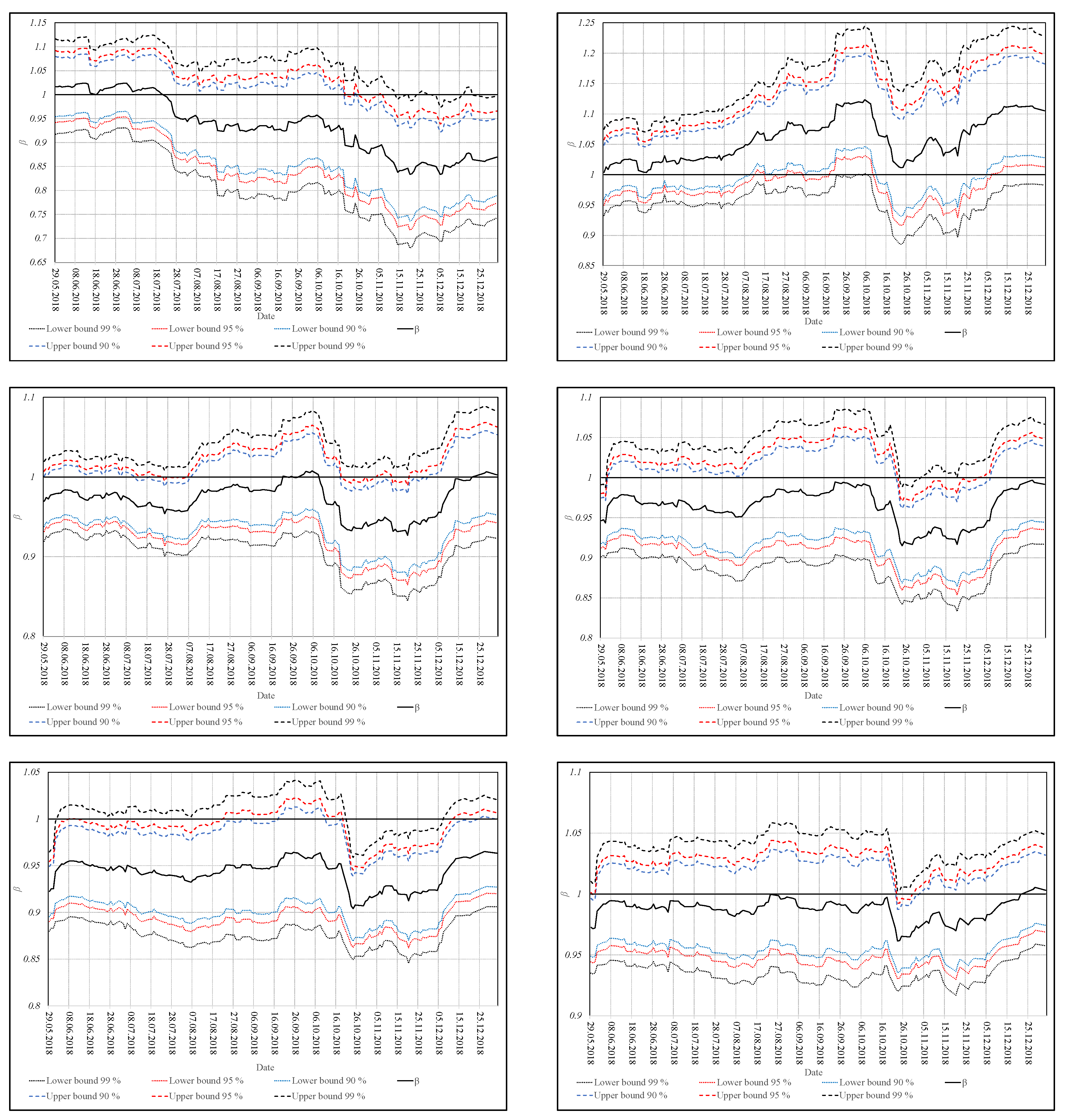
In Figure 1, we plot the power of the suggested test as a function of δ for n { 60 , 120 , 250 , 500 } . We observe that even for a small sample size, like n = 60 , the test is able to reject the null hypothesis already for small deviations from the target value β 0 . For instance, the power of the test is larger than 60% when δ is around 0.3 only, and it is approximately equal to 1 if δ = 0.6 . Furthermore, the power of the test increases as the sample size becomes larger. For instance, the power is around 1 already for δ close to 0.3 when n = 250 and for δ around 0.2 when n = 500 .

3. Empirical Illustration

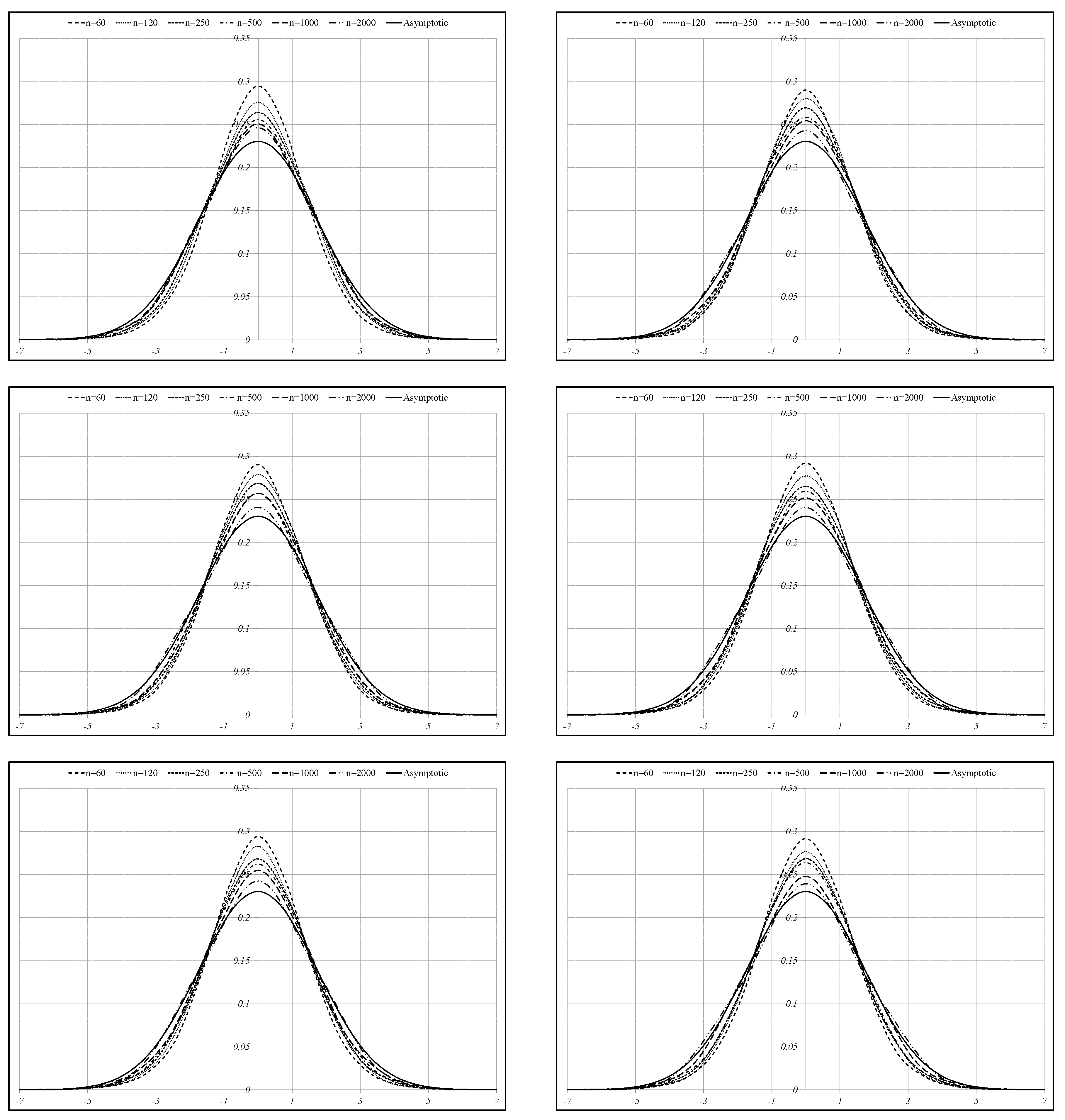
In this section, we implement the theoretical findings of Section 2 to real data based on the daily returns on the assets included into the DAX index for the period from 1st January 2018 to 31st December 2018 (251 observations). As a benchmark portfolio w b , the DAX index is chosen whose weights are provided on the official website of the German capital market, namely, on www.boerse.de. As a target portfolio for which we aim to infer the beta coefficient, we take the equally-weighted portfolio of six dimensions, namely, k { 5 , 10 , 15 , 20 , 25 , 30 } , which consists of the corresponding first k assets included into the DAX index in alphabetical order. Using the running window with length equal to n = 100 , we constructed confidence intervals for six considered equally-weighted portfolios at significance level 1 γ { 90 % , 95 % , 99 % } and have plotted them in Figure 2.
In Figure 2, we observe that the beta coefficient of the equally-weighted portfolios does not deviate considerably from one for almost all of the considered dimensions. The smallest values of the beta coefficient are present in the case of the k = 5 dimensional equally-weighted portfolio, especially at the end of 2018, where the estimated beta coefficient drops to 0.85 . By contrast, the beta coefficient is almost always larger than the one for the k = 10 dimensional portfolio. When the portfolio dimension increases, then the beta coefficient becomes less volatile in time. For instance, almost all values of β ^ belong to the interval [ 0.96 , 1 ] when k = 30 . Finally, the beta coefficients of the equally-weighted portfolios drop at the second part of October 2018, which is in-line with the opinion that October 2018 was the worst month in more than six years (since May 2012) for global capital markets since the global financial crisis in 2008. Some events, like disappointing earnings from big tech companies and a budget row between Italy and the European Union, seem to have a large influence on the overall performance of the German capital market.
Finally, confidence intervals constructed for the beta coefficients of the considered equally-weighted portfolios cover one in almost all of the considered cases with the exception present during several weeks in October 2018–December 2018 for the k = 5 , for the k = 25 , and for the k = 30 dimensional equally-weighted portfolio. At the end of 2018, the estimated beta coefficients increase, and only the confidence intervals constructed for the 5-dimensional portfolio do not include the value of one.

4. Robustness to the Violation of the Normality Assumption

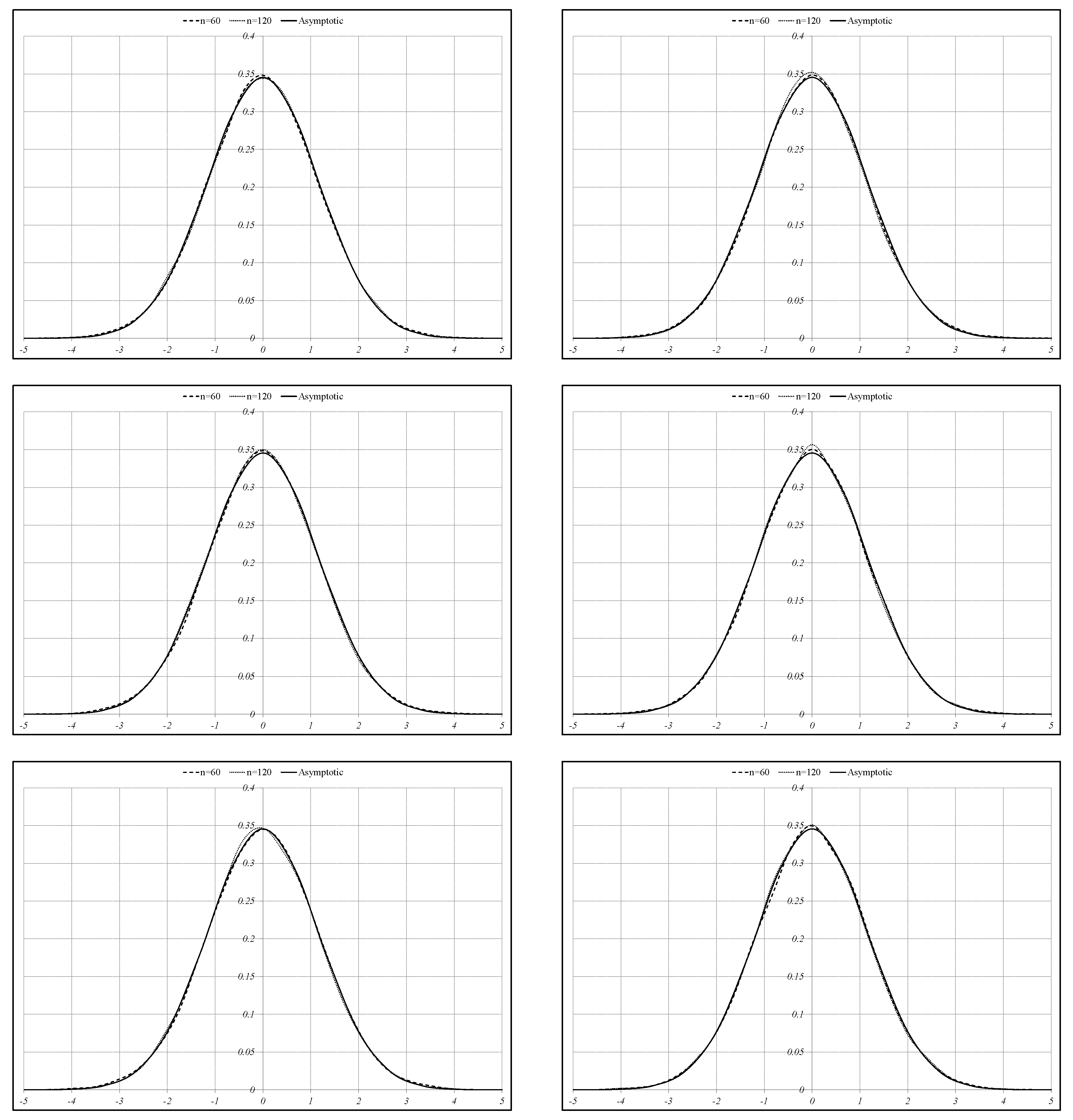
The theoretical findings of Section 3 were obtained under the assumption that the asset returns are normally distributed. In this section, we investigate how crucial the assumption of normality is on the performance of the beta estimator and on the distributional properties of the test statistic T introduced in Section 2.2. The results were obtained via a Monte Carlo study by drawing a random sample of size n from the k-dimensional multivariate t-distribution with d { 5 , 10 } degrees of freedom. Several values of k and n are considered, namely, k { 5 , 10 , 15 , 20 , 25 , 30 } and n { 60 , 120 , 250 , 500 , 1000 , 2000 } . For each possible choice of ( k , n ) , we drew a sample from the t-distribution with 5 and 10 degrees of freedom, with the location vector and covariance matrix equal to the sample mean vector and to the sample covariance matrix computed from the daily returns on the assets included into the DAX index for the period from 1st January 2018 to 31st December 2018 (251 observations). From the simulated data, the standardized realization of the estimated beta coefficient was computed as well as the value of the test statistic T provided in Section 2.2. Finally, the whole procedure was repeated B = 50,000 times for each possible value of d, k, and n. The resulting samples of the standardized estimators of the beta coefficient and of the values of the test statistic T were used to estimate their sampling distribution by employing the kernel density estimator with Epanechnikov kernel.
In Figure 3 and Figure 4, the results are shown for the t-distribution with 5 and 10 degrees of freedom. In both figures, we present the kernel density estimators and the asymptotic density of the standardized estimator for the beta coefficient given by:
n 1 β ^ β σ 2 / σ b 2 β 2 d N ( 0 , 1 ) ,
with:
σ 2 = w Σ w and σ b 2 = w b Σ w b .
and note that similar results are also present for the values of the test statistic T. The plots in the case of T are not included in the paper and are available from the corresponding author on request. Independently of the sample size, the kernel densities of the standardized estimator for the beta coefficient are roughly symmetric around zero. Small departures from the asymptotic distribution, which is the standard normal distribution, are present in the case of kernel densities computed when the sample size is relatively small and asset returns are generated from the t-distribution with 5 degrees of freedom. If data are generated from the t-distribution with 10 degrees of freedom, then the convergence of the kernel densities is already observed for a small sample size equal to 120, and for that reason, the kernel densities computed for large sample size are not present in Figure 4.

5. Summary

The capital asset pricing model is one of the most popular approaches in financial literature to model the trade-off between portfolio (asset) return and risk, which was independently introduced by Sharpe (1964), Lintner (1965), and Mossin (1966). The model equation relates the asset return to the market return by a linear function whose slope is known as the beta coefficient. As a result, the beta coefficient possesses several interesting and important properties in finance, one of which is the ability to capture the risk of a portfolio/security.
From an econometrical point of view, the CAPM can also be considered as a one-factor model or as a linear regression model whose parameters can be estimated by ordinary least square method (cf. Greene 2003; Dhrymes 2017). This approach, in particular, allows obtaining the point estimator of the portfolio beta coefficient. On the other hand, the return of the market portfolio is not a deterministic variable as usually assumed in the setup of the regression model, but it is a random quantity whose randomness should be taken into account when a confidence interval for the population beta coefficient is constructed or the corresponding test theory is developed. We deal with this point in the present paper by employing methods of multivariate statistical analysis. This procedure allows studying the distributional properties of the estimated beta coefficient by deriving its finite-sample density function and by introducing an exact test for the population beta coefficient. Furthermore, the distribution of the suggested test statistic is derived under both the null hypothesis and the alternative hypothesis. While the results obtained under the null hypothesis can be used to construct the rejection region of the test, the findings under the alternative hypothesis provide information about the power of the suggested test.
The derived theoretical results are not only restricted to the study of the stochastic properties of the estimated beta coefficient, but they are also applicable in the general theory of the linear models with stochastic regressors. As such, they discover a statistical approach based on the distributional properties of the Wishart distribution which might be applicable in different problems dealing with models where the independent variables are stochastic. Although we deal only with one stochastic factor, an extension to the general case with an arbitrary fixed number of stochastic independent variables can be dealt with in a similar way. Thus, the developed theory for the CAPM can be further extended to another popular linear model in financial literature, namely, the arbitrage pricing theory (see, e.g., Ross 1976).

Author Contributions

Investigation: T.B., A.K.G., V.V. and T.Z.; Writing original draft, T.B., A.K.G., V.V. and T.Z.

Funding

This research received no external funding.

Acknowledgments

The authors are thankful to Ivan Wang and four anonymous Reviewers for careful reading of the paper and for their suggestions, which improved an earlier version of this paper.

Conflicts of Interest

The authors declare no conflict of interest.

References

  1. Aitchison, John. 1964. Confidence-region tests. Journal of the Royal Statistical Society: Series B (Methodological) 26: 462–76. [Google Scholar] [CrossRef]
  2. Alexander, Carol. 2001. Market Models: A Guide to Financial Data Analysis. Hoboken: John Wiley & Sons. [Google Scholar]
  3. Alexander, Gordon J., and Alexandre M. Baptista. 2002. Economic implications of using a mean-var model for portfolio selection: A comparison with mean-variance analysis. Journal of Economic Dynamics and Control 26: 1159–93. [Google Scholar] [CrossRef]
  4. Alexander, Gordon J., and Alexandre M. Baptista. 2004. A comparison of var and cvar constraints on portfolio selection with the mean-variance model. Management Science 50: 1261–73. [Google Scholar] [CrossRef]
  5. Bauder, David, Rostyslav Bodnar, Taras Bodnar, and Wolfgang Schmid. 2019. Bayesian estimation of the efficient frontier. Scandinavian Journal of Statistics. forthcoming. [Google Scholar] [CrossRef]
  6. Berk, Jonathan B. 1997. Necessary conditions for the capm. Journal of Economic Theory 73: 245–57. [Google Scholar] [CrossRef]
  7. Bodnar, Taras, Wolfgang Schmid, and Tara Zabolotskyy. 2012. Minimum var and minimum cvar optimal portfolios: Estimators, confidence regions, and tests. Statistics & Risk Modeling with Applications in Finance and Insurance 29: 281–314. [Google Scholar]
  8. Bodnar, Taras, and Wolfgang Schmid. 2009. Econometrical analysis of the sample efficient frontier. The European Journal of Finance 15: 317–35. [Google Scholar] [CrossRef]
  9. Bodnar, Taras, Nestor Parolya, and Wolfgang Schmid. 2018. Estimation of the global minimum variance portfolio in high dimensions. European Journal of Operational Research 266: 371–90. [Google Scholar] [CrossRef]
  10. Damodaran, Aswath. 2012. Investment Valuation: Tools and Techniques for Determining the Value of any Asset. Hoboken: John Wiley & Sons. [Google Scholar]
  11. Dhrymes, Phoebus. 2017. Introductory Economerics. Berlin: Springer. [Google Scholar]
  12. Frahm, Gabriel, and Christoph Memmel. 2010. Dominating estimators for minimum-variance portfolios. Journal of Econometrics 159: 289–302. [Google Scholar] [CrossRef]
  13. Gibbons, Michael R., Stephen A. Ross, and Jay Shanken. 1989. A test of the efficiency of a given portfolio. Econometrica 57: 1121–52. [Google Scholar] [CrossRef]
  14. Greene, William H. 2003. Econometric Analysis. Chennai: Pearson Education India. [Google Scholar]
  15. Gupta, Arjun K., Tamas Varga, and Taras Bodnar. 2013. Elliptically Contoured Models in Statistics and Portfolio Theory. New York: Springer. [Google Scholar]
  16. Hodgson, Douglas J., Oliver Linton, and Keith Vorkink. 2002. Testing the capital asset pricing model efficiently under elliptical symmetry: A semiparametric approach. Journal of Applied Econometrics 17: 617–39. [Google Scholar] [CrossRef]
  17. Lintner, John. 1965. The valuation of risk assets and the selection of risky investments in stock portfolios and capital budgets. The Review of Economics and Statistics 47: 13–37. [Google Scholar] [CrossRef]
  18. Markowitz, Harry. 1952. Portfolio selection. The Journal of Finance 7: 77–91. [Google Scholar]
  19. Merton, Robert C. 1972. An analytic derivation of the efficient portfolio frontier. Journal of Financial and Quantitative Analysis 7: 1851–72. [Google Scholar] [CrossRef]
  20. Mossin, Jan. 1966. Equilibrium in a capital asset market. Econometrica: Journal of the Econometric Society 34: 768–83. [Google Scholar] [CrossRef]
  21. Muirhead, Robb J. 1982. Aspects of Multivariate Statistical Theory. New York: Wiley. [Google Scholar]
  22. Ross, Stephen A. 1976. The arbitrage theory of capital asset pricing. Journal of Economic Theory 13: 341–60. [Google Scholar] [CrossRef]
  23. Schmid, Wolfgang, and Taras Zabolotskyy. 2008. On the existence of unbiased estimators for the portfolio weights obtained by maximizing the sharpe ratio. AStA Advances in Statistical Analysis 92: 29–34. [Google Scholar] [CrossRef]
  24. Sharpe, William F. 1964. Capital asset prices: A theory of market equilibrium under conditions of risk. The Journal of Finance 19: 425–42. [Google Scholar]
  25. Sharpe, William F. 1994. The sharpe ratio. Journal of Portfolio Management 21: 49–58. [Google Scholar] [CrossRef]
  26. Zhou, Guofu. 1993. Asset-pricing tests under alternative distributions. The Journal of Finance 48: 1927–42. [Google Scholar] [CrossRef]
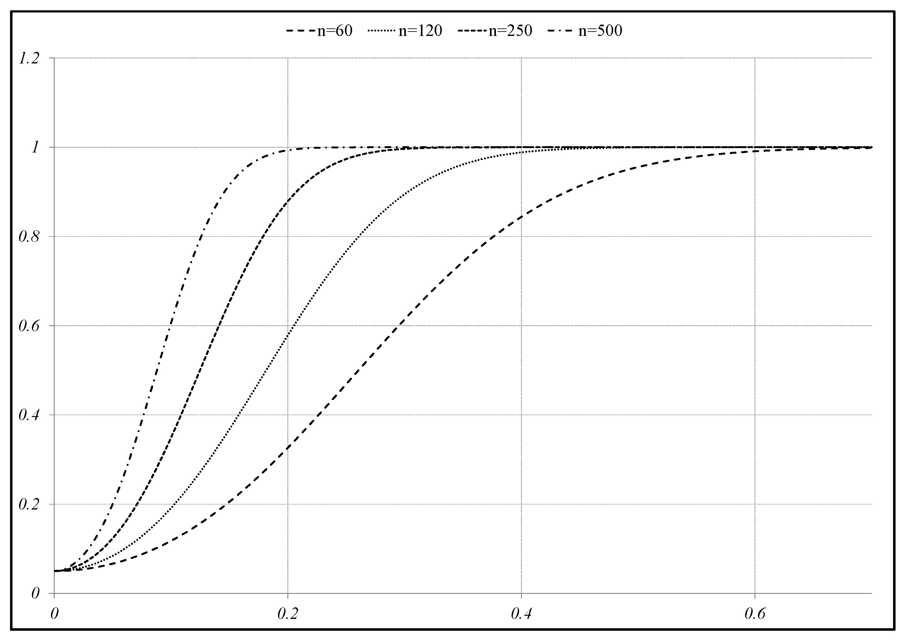
Figure 1. Power function for n { 60 , 120 , 250 , 500 } and γ = 0.05 .
Risks 07 00056 g001
Figure 2. Sample estimators and confidence intervals for the beta coefficient of the equally-weighted portfolio constructed for the first k = 5 (top left), k = 10 (top right), k = 15 (middle left), k = 20 (middle right), k = 25 (bottom left), and k = 30 (bottom right) assets included into the DAX index in alphabetical order.
Risks 07 00056 g002
Figure 3. Kernel density estimators for n { 60 , 120 , 250 , 500 , 1000 , 2000 } and the asymptotic density of the standardized estimator for the beta coefficient in the case of the k = 5 (top left), k = 10 (top right), k = 15 (middle left), k = 20 (middle right), k = 25 (bottom left), and k = 30 (bottom right) dimensional equally-weighted portfolio. The asset returns are drawn from the multivariate t-distribution with 5 degrees of freedom.
Risks 07 00056 g003
Figure 4. Kernel density estimators for n { 60 , 120 } and the asymptotic density of the standardized estimator for the beta coefficient in the case of the k = 5 (top left), k = 10 (top right), k = 15 (middle left), k = 20 (middle right), k = 25 (bottom left), abd k = 30 (bottom right) dimensional equally-weighted portfolio. The asset returns are drawn from the multivariate t-distribution with 10 degrees of freedom.
Risks 07 00056 g004