A General Framework for Portfolio Theory. Part III: Multi-Period Markets and Modular Approach

Abstract

This is Part III of a series of papers which focus on a general framework for portfolio theory. Here, we extend a general framework for portfolio theory in a one-period financial market as introduced in Part I [Maier-Paape and Zhu, Risks 2018, 6(2), 53] to multi-period markets. This extension is reasonable for applications. More importantly, we take a new approach, the “modular portfolio theory”, which is built from the interaction among four related modules: (a) multi period market model; (b) trading strategies; (c) risk and utility functions (performance criteria); and (d) the optimization problem (efficient frontier and efficient portfolio). An important concept that allows dealing with the more general framework discussed here is a trading strategy generating function. This concept limits the discussion to a special class of manageable trading strategies, which is still wide enough to cover many frequently used trading strategies, for instance “constant weight” (fixed fraction). As application, we discuss the utility function of compounded return and the risk measure of relative log drawdowns.

1. Introduction

This is Part III of a series of papers which focus on a general framework for portfolio theory. We laid out a general framework for portfolio theory in a one-period financial market for trading-off between reward and risk in Part I (Maier-Paape and Zhu 2018a) and addressed specifically drawdown risk measures in Part II (Maier-Paape and Zhu 2018b). Furthermore, a fourth part is planned where we provide a case study on how to implement the general framework in real financial markets. Here, in Part III, we extend the general framework for one-period financial markets to multi-period financial markets and go beyond the setting of a finite sample space.

In addition to extending the framework in Part I (Maier-Paape and Zhu 2018a) to more general settings, we now take a modular approach in organizing this more general framework for portfolio/trading theory. We recognize the problem of trading-off between higher reward and lower risk using portfolio/trading strategies within four modular blocks (modular portfolio theory): (a) multi-period market model; (b) trading strategies; (c) risk and utility functions; and (d) the optimization problem.

The multi-period market is assumed to consist of one risk-free and $M\in \mathbb{N}$ risky assets. The trading strategy is parameter dependent and specifies how the investor, once started the investment, wants to trade the portfolio over time. Based on this, a (convex) risk function $\mathfrak{r}$ and a (concave) reward/utility function $\mathfrak{u}$ can be defined, which manifest in an optimization problem of the form

$$\underset{x\in A}{min}\mathfrak{r}\left(x\right)\mathrm{subject}\mathrm{to}\mathfrak{u}\left(x\right)\ge \mu ,S_0^{\top }x=\beta ,$$

(1)

where $A\subset {\mathbb{R}}^{M+1}$, $\mu \in \mathbb{R}$ and $\beta >0$ are fixed and $S_0\in {\mathbb{R}}^{M+1}$ gives the initial price values of the $M+1$ assets. This just sketches the situation discussed here. Especially the role of the trading strategy and the meaning of the vector $x\in {\mathbb{R}}^{M+1}$ are discussed in more detail below.

Using a one-period market, there is nothing to do in Block (b) because the portfolio just consists of a simple portfolio vector x, which gives the weights. This one-period case is extensively studied in the literature. One of the first discussions on optimization problems of the form of Equation (1) was done by Markowitz (1952, 1959), the so-called modern portfolio theory, and afterwards with the capital asset pricing model (CAPM) by Lintner (1965); Mossin (1966); Sharpe (1964). In both settings, the risk function is defined by the standard deviation of the returns of the portfolio and the utility function is the mean return of the portfolio. The only part which can be chosen in this work could be the specific one-period market model because Block (b) is trivial, Block (c) is already fixed and Block (d) is of the form of Equation (1), in general with $A={\mathbb{R}}^{M+1}$. Decades later, Rockafellar et al. (2006) and also Part I (Maier-Paape and Zhu 2018a) discussed a more general setting where Block (c) gets more degrees of freedom regarding the choice of the risk function and the utility function. In Rockafellar et al. (2006), the risk function is allowed to be more general with some specific assumptions, so-called deviation measures, but the utility function still is the (arithmetic) mean return. In Maier-Paape and Zhu (2018a), in addition, the utility function is of more general form with some reasonable assumptions and the one-period market model is assumed to be defined on a finite probability space. In both cases the optimization problem is of the form of Equation (1) as well. The idea of using a multi-period market model together with trading strategies as building blocks for a modular portfolio theory was firstly introduced by Platen (2018). Accordingly, we here enhance on this idea and develop an in itself complete and compact approach to this new aspect of portfolio theory. Of course, multi-period market models have been used before, though not in the context of portfolio theory. For an introduction to this topic we refer to (Föllmer and Schied 2016, Section 5.1) and also (Carr and Zhu 2018, Chapter 3).

The generalization to multi-period markets for portfolio purposes is important in applications. In practice, investors and regulators always need to make decisions at different phases of financial markets under different policy environments. Moreover, many important market operations such as hedging and pricing of options and other contingent claims have to be dealt with in a multi-period financial market setting. Finally, the multi-period financial market model is crucial in adequately modeling certain important reward and risk measures such as compounded return and drawdown related risk measures. The absolute drawdown was already discussed, e.g., by Chekhlov et al. (2003, 2005); Goldberg and Mahmoud (2017) and Zabarankin et al. (2014). The risk functions used therein are based on the ideas of the value at risk but applied to the absolute drawdown. The relative drawdown is much more involved and rarely discussed in the literature. Grossman and Zhou (1993) studied an optimization problem using the maximum relative drawdown and a geometric Brownian motion with drift as market model where just one risky and also one risk-free asset are assumed. Cvitanić and Karatzas (1995) extended the results for more than one risky asset and Cherny and Obłój (2013) discussed the setting using an abstract semimartingale financial market and more general utility and risk functions. Properties on the mean of the logarithm of the relative drawdown are discussed in Part II (Maier-Paape and Zhu 2018b), where a one-period market model is used with a finite probability space and independent and identically distributed returns. The trick to construct the drawdown measure is to generate short equity curves by random drawings from the return distribution and to subsequently calculate the drawdowns of the equity curves. The relative drawdown for a more general market model was also discussed by Platen (2018).

A more technical challenge of our extension is that the space of random variables on the sample space that represents the payoff is no longer a finite dimensional space and, therefore, no longer enjoys local compactness properties. We circumvent this difficulty by introducing a trading strategy generating function. Doing so, we limit ourselves to a special class of manageable trading strategies. We illustrate by examples that the class of trading strategies we study here is wide enough to include many frequently used trading strategies such as “buy and hold” or “constant weight” (fixed fractions). Another strategy could be to fix the amount of money invested over time, which was discussed by Platen (2018). Although the here used strategies seem to be simple, it still shows the potential behind this new building block in portfolio theory.

The paper is arranged as follows. In Section 2, we layout the multi-period market models (Building Block (a)) and trading strategies (Building Block (b)) and derive several basic properties such as the fundamental characterization of a multi-period market with no nontrivial risk-free trading strategy (see Theorem 1). In Section 3, we discuss our main results according to the modular approach. After giving examples for the risk and utility functions (Building Block (c)) based on Blocks (a) and (b) in Section 3.1, the optimization problem (Building Block (d)) is introduced in Section 3.2. The corresponding notion of efficient frontier is extensively studied, e.g., in terms of graphs (see Section 3.3) and the main theorems for the existence (and uniqueness) of solutions are derived in Section 3.4. An application of the theory for the compounded return and the expected log relative drawdown is discussed in detail in Section 4. To measure the return in risk and utility function as relative log returns has two reasons. Firstly, it yields the necessary convexity and concavity, respectively. Secondly, it guarantees that drawdowns and runups are measured equally. For instance, a drawdown of $50\%$ needs a runup of $100\%$ for compensation. Taking log relative returns, the absolute value of both movements is equal. The paper ends with some conclusions in Section 5.

Before we continue, we would like to emphasize once more that this Part III is an advancement of Parts I and II Maier-Paape and Zhu (2018a, 2018b). Although this Part III is self-contained, complications stemming from the multi-period market model and the general probability space make this Part III more involved. Therefore, the reader might it find helpful to compare results here with the “easy” case in Parts I and II (see Maier-Paape and Zhu (2018a, 2018b)). For instance, the “core” theory here on optimization problems such as in Equation (1) and efficient portfolios is very much in the spirit of Part I (Maier-Paape and Zhu 2018a) (cf. Section 3.2, Section 3.3 and Section 3.4). Similarly, Section 3.1 and Section 4, where we lift the drawdown risk measures to multi-period markets, use many ideas of Part II (Maier-Paape and Zhu 2018b). On the other hand, the contents of Section 2 on theory of multi-period markets and trading strategies has no counterpart in Parts I and II Maier-Paape and Zhu (2018a, 2018b) but many connections to classical financial mathematics (e.g., Föllmer and Schied (2016)). As a matter of fact, Section 2 is a bit technical. However, since it only provides the framework for the core theory later on, it might help at first reading to concentrate oneself in Section 2 solely on the definitions.

2. Multi-Period Market and Trading Strategies

In this section, we describe a multi-period (financial) market model. In such a model, investment decisions are made over several periods with potentially different investment environments characterized by different economic, financial and policy situations. The role of portfolios is replaced by trading strategies which can be viewed as a sequence of portfolios varying in time according to an a priori given, but possibly random, strategy. The information on the investment environment is revealed with the progress of time and the action of the trading strategy is contingent on the existing information. The availability of the information is modeled by a filtration. This section lays a foundation for the subsequent analysis.

2.1. Definitions

The following notion of a multi-period market is closely related to (Föllmer and Schied 2016, Section 5.1) and (Platen 2018, Sections 2.1.2, 2.2.1, and 2.2.2). We assume that $M+1$ financial instruments (one risk-free asset with index 0 and $M\in \mathbb{N}$ risky assets with indexes $1,\dots ,M$) are given. Their initial prices are denoted by $S_0:=(S_0^0,S_0^1,\dots ,S_0^M)\in {\mathbb{R}}_{>0}^{M+1}$. A model for $N\in \mathbb{N}$ future time steps is of the following form:

Let $(\Omega ,\Sigma ,\mathrm{P})$ be a probability space. By ${\mathcal{L}}^2:={\mathcal{L}}^2(\Omega ,\Sigma ,\mathrm{P}):={\mathcal{L}}^2(\Omega ,\Sigma ,\mathrm{P};{\mathbb{R}}^{})$ we denote the set of all random variables $X:\Omega \to \mathbb{R}$ with finite norm ${∥X∥}_{{\mathcal{L}}^2}:={(E[X^2\left]\right)}^{1/2}$, where ${⟨X,Y⟩}_{{\mathcal{L}}^2}:=E\left[XY\right]$ for $X,Y\in {\mathcal{L}}^2$ is the inner product. For a set of $M+1$ assets, we define ${\mathcal{L}}^2(\Omega ,\Sigma ,\mathrm{P};{\mathbb{R}}^{M+1})$ where each of the $M+1$ components of the elements are in ${\mathcal{L}}^2$. This could model a one-period market. For a multi-period market model, let $(\Omega ,\Sigma ,{\left\{{\mathcal{F}}_n\right\}}_{0\le n\le N},\mathrm{P})$ be a filtered probability space with filtration ${\left\{{\mathcal{F}}_n\right\}}_{0\le n\le N}$ which satisfies

$$\{\varnothing ,\Omega \}=:{\mathcal{F}}_0\subset {\mathcal{F}}_1\subset \cdots \subset {\mathcal{F}}_{N-1}\subset {\mathcal{F}}_N:=\Sigma .$$

Define

$${\mathcal{L}}^2(N;{\mathbb{R}}^M):={\mathcal{L}}^2(\Omega ,\Sigma ,{\left\{{\mathcal{F}}_n\right\}}_{0\le n\le N},\mathrm{P};{\mathbb{R}}^M):=\underset{n=0}{\overset{N}{✕}}{\mathcal{L}}^2(\Omega ,{\mathcal{F}}_n,\mathrm{P};{\mathbb{R}}^M)$$

and ${\mathcal{L}}^2\left(N\right):={\mathcal{L}}^2(N;{\mathbb{R}}^{})$ with corresponding set of positive processes

$${\mathcal{L}}^2(N;{\mathbb{R}}_{>0}^M):={\mathcal{L}}^2(\Omega ,\Sigma ,{\left\{{\mathcal{F}}_n\right\}}_{0\le n\le N},\mathrm{P};{\mathbb{R}}_{>0}^M):=\underset{n=0}{\overset{N}{✕}}{\mathcal{L}}^2(\Omega ,{\mathcal{F}}_n,\mathrm{P};{\mathbb{R}}_{>0}^M)\subset {\mathcal{L}}^2(N;{\mathbb{R}}^M).$$

Analogously, ${\mathcal{L}}^0$ denotes the set of all random variables and ${\mathcal{L}}^1$ the random variables with finite (absolute) expectation. In most cases, we use ${\mathcal{L}}^2$, which, however, often is not required. In these cases, one could also use, e.g., ${\mathcal{L}}^0$.

Firstly, we define the notion of risk-free which means that there is no uncertainty and the price development is (not necessarily strictly) monotone increasing.

Definition 1 (Risk-free asset).

The stochastic process $Z:=(Z_0,Z_1,\dots ,Z_N)\in {\mathcal{L}}^{2}N$ is called risk-free if $Z_n$ is constant almost surely (a.s.) for $n=0,1,\dots ,N$ and $Z_n\ge Z_{n-1}>0$ a.s. for $n=1,\dots ,N$.

Definition 2 

(Multi-period market model, cf. (Föllmer and Schied 2016, Section 5.1)). For $M\in \mathbb{N}$ let $S:={\left(S_n\right)}_{0\le n\le N}\in {\mathcal{L}}^2(N;{\mathbb{R}}_{>0}^{M+1})$ with

$$S_n:={\left(S_n^0,S_n^1,\dots ,S_n^M\right)}^{\top }\in {\mathbb{R}}_{>0}\times {\mathcal{L}}^2\left(\Omega ,{\mathcal{F}}_n,\mathrm{P};{\mathbb{R}}_{>0}^M\right)\subset {\mathcal{L}}^2\left(\Omega ,{\mathcal{F}}_n,\mathrm{P};{\mathbb{R}}_{>0}^{M+1}\right),$$

(2)

where $(S_0^0,S_1^0,\dots ,S_N^0)\in {\mathcal{L}}^2\left(N\right)$, i.e., the asset with index zero, is risk-free. The stochastic process S is called a multi-period market model of size $M+1$ with N time steps.

A portfolio in a one-period market model just contains of a single vector which gives the weights for each asset. In a multi-period market model the situation is much more complex. After each time step we can change the weights. We even can change the weights, say after time step n, based on information of all past time steps up to step n. Hence, in our situation, we denote a series of time varying portfolios by a trading strategy as follows.

Definition 3 (Trading strategy).

For $M,N\in \mathbb{N}$ let $S:={\left(S_n\right)}_{0\le n\le N}\in {\mathcal{L}}^2(N;{\mathbb{R}}_{>0}^{M+1})$ be a market model. A time dependent vector

$$X:={\left(x_n\right)}_{1\le n\le N}\in {\mathcal{L}}^0\left(N-1;{\mathbb{R}}^{M+1}\right):=\underset{n=0}{\overset{N-1}{✕}}{\mathcal{L}}^0\left(\Omega ,{\mathcal{F}}_n,\mathrm{P};{\mathbb{R}}^{M+1}\right),$$

for the same filtered probability space $(\Omega ,\Sigma ,{\left\{{\mathcal{F}}_n\right\}}_{0\le n\le N},\mathrm{P})$ from the market model, with

$$x_n:={\left(x_n^0,x_n^1,\dots ,x_n^M\right)}^{\top }\in {\mathcal{L}}^0\left(\Omega ,{\mathcal{F}}_{n-1},\mathrm{P};{\mathbb{R}}^{M+1}\right),$$

(3)

for $n=1,\dots ,N$, is called a trading strategy.

We still need to give the trading strategy a meaning and a real connection to the market model S. The values of a trading strategy $X={\left(x_n\right)}_{1\le n\le N}$ have the following interpretation:

• $x_n$ may depend on $S_0,\dots ,S_{n-1}$ but not on later prices;
• $S_n^i$ absolute price of the ith asset at time n;
• $x_n^i$: number of shares invested into the ith asset from time step $n-1$ to n;
• $S_{n-1}^i{x}_n^i$: amount of money invested into the ith asset;
• $S_n^i{x}_n^i$: absolute value of this investment after the time step from $n-1$ to n; and
• $S_n^{\top }{x}_n={\sum }_{i=0}^M{S}_n^i{x}_n^i$: absolute value of all investments after the time step from $n-1$ to n.

Note that Equations (2) and (3) imply that $S_n$ is ${\mathcal{F}}_n$ measurable while $x_n$ is ${\mathcal{F}}_{n-1}$ measurable. The reason is that $x_n$ are the number of shares for each asset hold from time step $n-1$ to n. This must be known at time step $n-1$ where the shares have to be bought. Hence, it must be ${\mathcal{F}}_{n-1}$ measurable. The prices $S_n$, of course, are known not before time n, i.e., it must be ${\mathcal{F}}_n$ measurable. Using this, we can define the wealth process realized by a trading strategy applied to the market model.

Definition 4 (Wealth of trading strategy).

Let $S\in {\mathcal{L}}^2(N;{\mathbb{R}}_{>0}^{M+1})$ be a market model and ${\mathcal{W}}_0\in {\mathbb{R}}_{>0}$ the investor’s fixed initial wealth. For a trading strategy $X={\left(x_n\right)}_{1\le n\le N}\in {\mathcal{L}}^0(N-1;{\mathbb{R}}^{M+1})$, the wealth process$\mathcal{W}\left(X\right)\in {\mathcal{L}}^0\left(N\right)$ is defined by

$$\begin{array}{cc}{\mathcal{W}}_0\left(X\right)\hfill & :={\mathcal{W}}_0\hfill \\ {\mathcal{W}}_n\left(X\right)\hfill & :={\mathcal{W}}_n\left(x_1,\dots ,x_n\right):={\mathcal{W}}_{n-1}\left(X\right)+{\left(S_n-S_{n-1}\right)}^{\top }{x}_n={\mathcal{W}}_0+\sum _{k=1}^n{\left(S_k-S_{k-1}\right)}^{\top }{x}_k\hfill \end{array}$$

(4)

for $n=1,\dots ,N$. Hence, $\mathcal{W}:{\mathcal{L}}^0(N-1;{\mathbb{R}}^{M+1})\to {\mathcal{L}}^0\left(N\right)$ is an affine linear functional.

Note, that, whenever $X\in {\mathcal{L}}^2(N-1;{\mathbb{R}}^{M+1})$, then, by the Cauchy–Schwarz inequality, we obtain that $\mathcal{W}\left(X\right)\in {\mathcal{L}}^1\left(N\right)$.

Even though the market model consists of positive stochastic processes, we may open short positions using a trading strategy. Hence, total ruin may occur. Since we always try to avoid a ruin, we define the set of admissible trading strategies.

Definition 5 (Admissible trading strategy).

A trading strategy X which satisfies ${\mathcal{W}}_n\left(X\right)>0$ a.s. for $n=1,\dots ,N$ is called admissible. The set of all admissible trading strategies is denoted by $\mathcal{A}=\mathcal{A}\left(S\right)\subset {\mathcal{L}}^0(N-1;{\mathbb{R}}^{M+1})$.

Note that $\mathcal{A}$ is a convex set.

2.2. Properties of the Multi-Period Market Model

The most important scenario we try to avoid is total ruin. This strongly depends on the trading strategy. However, the opposite should also be impossible, i.e., it should not be possible to gain money without risk, namely arbitrage. This property strongly depends on the market model itself. The literature mostly discusses the notion of arbitrage, where an arbitrage opportunity beats the risk-free asset with positive probability while it is never worse than the risk-free asset. In Part I (see (Maier-Paape and Zhu 2018a, Section 3.1)), the notion of a risk-free portfolio is introduced for the one-period market and a finite probability space. A risk-free portfolio is almost the same as an arbitrage opportunity but does not have to beat the risk-free asset with positive probability. We discuss this kind of extension for the more general case with multi-period market models (cf. also (Platen 2018, Section 2.2.3 and Section 2.2.4) for more details).

When discussing arbitrage, the notion of self-financing is often used (see, e.g., (Föllmer and Schied 2016, Definition 5.4)), which means that all money which has been invested initially stays invested and no fresh money is invested afterwards.

Definition 6 

(Self-financing, see (Föllmer and Schied 2016, Definition 5.4)). Let $S\in {\mathcal{L}}^2(N;{\mathbb{R}}_{>0}^{M+1})$ be a market model for $N\ge 2$. A trading strategy $X:={\left(x_n\right)}_{1\le n\le N}$ with

$$S_n^{\top }{x}_n=S_n^{\top }{x}_{n+1}$$

(5)

for all $n=1,\dots ,N-1$ is called self-financing.

The space of self-financing trading strategies is linear and simplifies the wealth process as follows.

Proposition 1.

Let $S\in {\mathcal{L}}^2(N;{\mathbb{R}}_{>0}^{M+1})$, $N\ge 2$, be a market model. A trading strategy X is self-financing if and only if

$${\mathcal{W}}_n\left(X\right)={\mathcal{W}}_0+\left(S_n^{\top }{x}_n-S_0^{\top }{x}_1\right)$$

(6)

for all $n=1,\dots ,N$. If $S_0^{\top }{x}_1={\mathcal{W}}_0$, then Equation (6) becomes ${\mathcal{W}}_n\left(X\right)=S_n^{\top }{x}_n$.

Proof. 

If X is self-financing, then Equation (4) becomes a telescoping sum and directly gives Equation (6). On the other hand, if Equation (6) holds true, then, by Equation (6), we get

$$\begin{array}{cc}{\mathcal{W}}_{n+1}\left(X\right)\hfill & ={\mathcal{W}}_0+\left(S_{n+1}^{\top }{x}_{n+1}-S_0^{\top }{x}_1\right)\hfill \end{array}$$

and, by Equation (4) together with Equation (6), we obtain

$$\begin{array}{cc}{\mathcal{W}}_{n+1}\left(X\right)\hfill & ={\mathcal{W}}_n\left(X\right)+{\left(S_{n+1}-S_n\right)}^{\top }{x}_{n+1}={\mathcal{W}}_0+\left(S_n^{\top }{x}_n-S_0^{\top }{x}_1\right)+{\left(S_{n+1}-S_n\right)}^{\top }{x}_{n+1}\hfill \end{array}$$

for $n=1,\dots ,N-1$. Equating both expressions gives $S_n{x}_n=S_n{x}_{n+1}$ for all $n=1,\dots ,N-1$, i.e., X is self-financing.□

Remark 1 (Bond).

Let $Z:={\left(z_n\right)}_{1\le n\le N}$ be the trading strategy which represents the bond, i.e.,

$$z_n:={\left(\frac{{\mathcal{W}}_0}{S_0^0},0,\dots ,0\right)}^{\top }\mathit{for}n=1,\dots ,N.$$

(7)

Of course, Z is self-financing with $S_0^{\top }{z}_1={\mathcal{W}}_0$. Therefore, Proposition 1 gives

$${\mathcal{W}}_n\left(Z\right)=S_n^{\top }{z}_n={\mathcal{W}}_0\frac{S_n^0}{S_0^0}\mathit{for}n=1,\dots ,N,$$

(8)

A trading strategy X is called trivial, if $\widehat{X}\equiv 0$ a.s., where $\widehat{X}:={\left({\widehat{x}}_n\right)}_{1\le n\le N}$ with ${\widehat{x}}_n:={(x_n^1,\dots ,x_n^M)}^{\top }$ denotes the risky part of X. Analogously, we define the risky part of $S:={\left(S_n\right)}_{0\le n\le N}$ by $\widehat{S}:={\left({\widehat{S}}_n\right)}_{0\le n\le N}$, where ${\widehat{S}}_n:={(S_n^1,\dots ,S_n^M)}^{\top }$.

The following notion of arbitrage opportunity, bond replicating and risk-free trading strategy is related to (Föllmer and Schied 2016, Definition 5.10), see (Platen 2018, Remark 2.2.17).

Definition 7 (Arbitrage opportunity, bond replicating, and risk-free).

Let $S\in {\mathcal{L}}^2(N;{\mathbb{R}}_{>0}^{M+1})$ for $M,N\in \mathbb{N}$ be a market model and $X:={\left(x_n\right)}_{1\le n\le N}$ a trading strategy.

(a) 

We say X is risk-free if

$$S_{n-1}^{\top }{x}_n\le {\mathcal{W}}_{n-1}\left(X\right)a.s.\mathit{for}\mathit{all}n=1,\dots ,N\mathit{and}{\mathcal{W}}_N\left(X\right)\ge {\mathcal{W}}_0\frac{S_N^0}{S_0^0}a.s.$$

(9)

We say market model S has no nontrivial risk-free trading strategy if there does not exist a risk-free trading strategy X with $\widehat{X}\not\equiv 0$ (i.e., besides the trivial ones with $\widehat{X}=0$ a.s. there are no risk-free trading strategies).

(b) 

We say X is an arbitrage opportunity if

$$S_{n-1}^{\top }{x}_n\le {\mathcal{W}}_{n-1}\left(X\right)a.s.\mathit{for}\mathit{all}n=1,\dots ,N,{\mathcal{W}}_N\left(X\right)\ge {\mathcal{W}}_0\frac{S_N^0}{S_0^0}a.s.,$$

and

$$\mathrm{P}\left({\mathcal{W}}_N\left(X\right)>{\mathcal{W}}_0\frac{S_N^0}{S_0^0}\right)>0.$$

We say market model S is arbitrage-free, if there does not exist any arbitrage opportunity.

(c) 

We say X is bond replicating if

$$S_{n-1}^{\top }{x}_n\le {\mathcal{W}}_{n-1}\left(X\right)a.s.\mathit{for}\mathit{all}n=1,\dots ,N\mathit{and}{\mathcal{W}}_N\left(X\right)={\mathcal{W}}_0\frac{S_N^0}{S_0^0}a.s.$$

We say market model S has no nontrivial bond replicating trading strategy, if there does not exist a bond replicating trading strategy X with $\widehat{X}\not\equiv 0$ (i.e., besides the trivial ones with $\widehat{X}=0$ a.s. there are no bond replicating trading strategies).

Remark 2 (Interpretation of Definition 7).

The first property of a risk-free trading strategy in Equation (9) says that, at time step $n-1$, no more than the available capital is invested. The second property in Equation (9) means that the final wealth of the trading strategy is always at least as much as the final wealth of the bond strategy according to Remark 1.

An arbitrage opportunity has the same properties, but on top of that the strategy wins strictly more than the bond strategy with positive probability.

A bond replicating trading strategy is also not allowed to invest more than the available capital. In this case, the final wealth has to be exactly the same as for the bond strategy.

The next result gives necessary and sufficient conditions for a market model having no nontrivial risk-free trading strategy. Those conditions are important when looking at properties for risk and utility measures on such market models. Another essential property regarding uniqueness is that two different trading strategies should result in two different wealth processes, which is ensured by the addition in the next result.

Theorem 1 (Multi-period market model with no nontrivial risk-free trading strategy).

The following assertions are equivalent:

(a) 

S has no nontrivial risk-free trading strategy.

(b) 

S is arbitrage-free and has no nontrivial bond replicating trading strategy.

(c) 

For all $n=1,\dots ,N$ and all $\mathit{\eta }\in {\mathcal{L}}^0(\Omega ,{\mathcal{F}}_{n-1},\mathrm{P};{\mathbb{R}}^{M+1})$ with $\widehat{\mathit{\eta }}\not\equiv 0$ it is

$$P\left({\left(S_n-\frac{S_n^0}{S_{n-1}^0}{S}_{n-1}\right)}^{\top }\mathit{\eta }<0\right)>0.$$

(10)

(d) 

S is arbitrage-free and the following holds for all trading strategies X and Y:

$$\mathcal{W}\left(X\right)=\mathcal{W}\left(Y\right)a.s.\mathit{implies}\widehat{X}=\widehat{Y}a.s.$$

(11)

If in addition $S_n^0>S_{n-1}^0$ for all $n=1,\dots ,N$ and one of the (a), (b), (c) or (d) holds, then the mapping $\mathcal{W}$ is injective, i.e., $\mathcal{W}\left(X\right)=\mathcal{W}\left(Y\right)$ a.s. implies $X=Y$ a.s.

Proof. 

The equivalence of (a) and (b) directly follows from Definition 7.

Proof of implication from (a) to (c): Assume this implication is wrong, i.e., assume there exist $n_0\in \{1,\dots ,N\}$ and ${\mathit{\eta }}^{*}\in {\mathcal{L}}^0(\Omega ,{\mathcal{F}}_{n_0-1},\mathrm{P};{\mathbb{R}}^{M+1})$ with ${\widehat{\mathit{\eta }}}^{*}\not\equiv 0$ such that

$$1=\mathrm{P}\left({\left(S_{n_0}-\frac{S_{n_0}^0}{S_{n_0-1}^0}{S}_{n_0-1}\right)}^{\top }{\mathit{\eta }}^{*}\ge 0\right)=\mathrm{P}\left({\left({\widehat{S}}_{n_0}-\frac{S_{n_0}^0}{S_{n_0-1}^0}{\widehat{S}}_{n_0-1}\right)}^{\top }{\widehat{\mathit{\eta }}}^{*}\ge 0\right),$$

(12)

or, equivalently, $S_{n_0}^{\top }{\mathit{\eta }}^{*}\ge (S_{n_0}^0/S_{n_0-1}^0)S_{n_0-1}^{\top }{\mathit{\eta }}^{*}$ a.s. Let trading strategy $Z:={\left(z_n\right)}_{1\le n\le N}$ represent the bond (see Remark 1). Define $Y:={\left(y_n\right)}_{1\le n\le N}$ by $y_{n_0}:={\mathit{\eta }}^{*}$ and $y_n:=z_n$ for $n\ne n_0$. Observe that for $1\le n\le n_0-1$ by Equation (8) now ${\mathcal{W}}_n\left(Y\right)={\mathcal{W}}_n\left(Z\right)={\mathcal{W}}_0{S}_n^0/S_0^0$ holds true. Since the property in Equation (12) of ${\mathit{\eta }}^{*}$ is independent on its risk-free part, we can choose, without loss of generality (w.l.o.g.), the bond part ${\eta }^0\in {\mathcal{L}}^0(\Omega ,{\mathcal{F}}_{n_0-1},\mathrm{P})$ of ${\mathit{\eta }}^{*}$ such that $S_{n_0-1}^{\top }{y}_{n_0}=S_{n_0-1}^{\top }{\mathit{\eta }}^{*}=S_{n_0-1}^0{\eta }^0+{\widehat{S}}_{n_0-1}^{\top }{\widehat{\mathit{\eta }}}^{*}={\mathcal{W}}_{n_0-1}\left(Y\right)={\mathcal{W}}_{n_0-1}\left(Z\right)=S_{n_0-1}^{\top }{z}_{n_0}$. For $n_0\le n\le N$, it follows from Equations (4), (7) and (8) that

$$\begin{array}{cc}{\mathcal{W}}_n\left(Y\right)\hfill & ={\mathcal{W}}_n\left(Z\right)-{\left(S_{n_0}-S_{n_0-1}\right)}^{\top }{z}_{n_0}+{\left(S_{n_0}-S_{n_0-1}\right)}^{\top }{\mathit{\eta }}^{*}\hfill \\ \hfill & ={\mathcal{W}}_0\frac{S_n^0}{S_0^0}-{\mathcal{W}}_0\frac{S_{n_0}^0-S_{n_0-1}^0}{S_0^0}+S_{n_0}^{\top }{\mathit{\eta }}^{*}-S_{n_0-1}^{\top }{\mathit{\eta }}^{*}\hfill \\ \hfill & \ge {\mathcal{W}}_0\frac{S_n^0}{S_0^0}-{\mathcal{W}}_0\frac{S_{n_0}^0-S_{n_0-1}^0}{S_0^0}+\frac{S_{n_0}^0}{S_{n_0-1}^0}{S}_{n_0-1}^{\top }{\mathit{\eta }}^{*}-S_{n_0-1}^{\top }{\mathit{\eta }}^{*}={\mathcal{W}}_0\frac{S_n^0}{S_0^0}={\mathcal{W}}_n\left(Z\right)\hfill \end{array}$$

(13)

holds a.s. and using $S_{n-1}^{\top }{y}_n=S_{n-1}^{\top }{z}_n={\mathcal{W}}_{n-1}\left(Z\right)$ one easily obtains with Equation (13) that $S_{n-1}^{\top }{y}_n\le {\mathcal{W}}_{n-1}\left(Y\right)$ a.s. for all $n=1,\dots ,N$. In particular, using Equation (13) for $n=N$, trading strategy Y must be risk-free and nontrivial. This contradicts (a). Hence, there cannot be such an ${\mathit{\eta }}^{*}$, i.e., (c) must hold.

Proof of implication from (c) to (a): Let (c) hold and assume there exists a nontrivial risk-free trading strategy $X:={\left(x_n\right)}_{1\le n\le N}$, i.e., X satisfies Equation (9) and $\widehat{X}\not\equiv 0$. Let $n_0\in \{1,\dots ,N\}$ be minimal with the property ${\widehat{x}}_{n_0}\not\equiv 0$. Before time $n_0$, trading strategy X can at most invest into the bond. Hence,

$$S_{n_0-1}^{\top }{x}_{n_0}\le {\mathcal{W}}_{n_0-1}\left(X\right)\le {\mathcal{W}}_0{S}_{n_0-1}^0/S_0^0\mathrm{a}.\mathrm{s}.$$

(14)

because of the first property in Equation (9). From (c) we get that $x_{n_0}$ satisfies Equation (10) for $\mathit{\eta }:=x_{n_0}$ and $n=n_0$. Hence, using Equations (4), (10) and (14), we obtain that the following holds true with positive probability:

$${\mathcal{W}}_{n_0}\left(X\right)={\mathcal{W}}_{n_0-1}\left(X\right)+{\left(S_{n_0}-S_{n_0-1}\right)}^{\top }{x}_{n_0}<{\mathcal{W}}_{n_0-1}\left(X\right)+\left(\frac{S_{n_0}^0}{S_{n_0-1}^0}-1\right)S_{n_0-1}^{\top }{x}_{n_0}\le {\mathcal{W}}_0\frac{S_{n_0}^0}{S_0^0}.$$

Because of the second property in Equation (9), it must be $n_0<N$ and there must exist a maximal $n_1\in \{n_0+1,\dots ,N\}$ such that

$$\mathrm{P}\left({\mathcal{W}}_{n_1-1}\left(X\right)<{\mathcal{W}}_0\frac{S_{n_1-1}^0}{S_0^0}\right)>0\mathrm{and}\mathrm{P}\left({\mathcal{W}}_{n_1}\left(X\right)\ge {\mathcal{W}}_0\frac{S_{n_1}^0}{S_0^0}\mid {\mathcal{W}}_{n_1-1}\left(X\right)<{\mathcal{W}}_0\frac{S_{n_1-1}^0}{S_0^0}\right)=1.$$

Define

$${\mathit{\eta }}^{\#}:=\left\{\begin{array}{cc}{x}_{n_1},\hfill & \mathrm{if}{\mathcal{W}}_{n_1-1}\left(X\right)<{\mathcal{W}}_0\frac{S_{n_1-1}^0}{S_0^0},\hfill \\ {\left({\mathcal{W}}_0/S_0^0,0,\dots ,0\right)}^{\top },\hfill & \mathrm{otherwise}.\hfill \end{array}\right.$$

Observe that ${\widehat{x}}_{n_1}\not\equiv 0$ and hence ${\widehat{\mathit{\eta }}}^{\#}\not\equiv 0$. Using Equations (4) and (9) it can then be shown that

$${\left(S_{n_1}-\frac{S_{n_1}^0}{S_{n_1-1}^0}{S}_{n_1-1}\right)}^{\top }{\mathit{\eta }}^{\#}={\left(S_{n_1}-S_{n_1-1}\right)}^{\top }{\mathit{\eta }}^{\#}-\frac{S_{n_1}^0-S_{n_1-1}^0}{S_{n_1-1}^0}{S}_{n_1-1}^{\top }{\mathit{\eta }}^{\#}\ge 0\mathrm{a}.\mathrm{s}.$$

which contradicts (c). Hence, S has no nontrivial risk-free trading strategy.

Proof of implication from (a)–(c) to (d): We just need to show Equation (11) for an arbitrage-free market S. Let $X:={\left(x_n\right)}_{1\le n\le N}$ and $Y:={\left(y_n\right)}_{1\le n\le N}$ fulfill $\mathcal{W}\left(X\right)=\mathcal{W}\left(Y\right)$ a.s. From Equation (4) it follows that ${(S_n-S_{n-1})}^{\top }(x_n-y_n)=0$ a.s. for $n=1,\dots ,N$. Now, let $n\in \{1,\dots ,N\}$ be arbitrary. W.l.o.g. it is $S_{n-1}^{\top }(x_n-y_n)\le 0$. Define ${\mathit{\eta }}^{†}:=x_n-y_n+{(c,0,\dots ,0)}^{\top }$ with $c:=-S_{n-1}^{\top }(x_n-y_n)/S_{n-1}^0\ge 0$. We have $S_{n-1}^{\top }{\mathit{\eta }}^{†}=0$ and therefore

$$0\le {\left(S_n-S_{n-1}\right)}^{\top }{\mathit{\eta }}^{†}={\left(S_n-\frac{S_n^0}{S_{n-1}^0}{S}_{n-1}\right)}^{\top }{\mathit{\eta }}^{†}\mathrm{a}.\mathrm{s}.$$

Because of (c), we then must have ${\widehat{\mathit{\eta }}}^{†}={\widehat{x}}_n-{\widehat{y}}_n\equiv 0$ a.s. Since n was arbitrary $\widehat{X}\equiv \widehat{Y}$ a.s. must hold, which proves Equation (11).

It remains to show the implication from (d) to (c): Since S is arbitrage-free, we firstly can show that for all $n=1,\dots ,N$ and all $\mathit{\eta }\in {\mathcal{L}}^0(\Omega ,{\mathcal{F}}_{n-1},\mathrm{P};{\mathbb{R}}^{M+1})$ with $\widehat{\mathit{\eta }}\not\equiv 0$ it is

$$\mathrm{P}\left({\left(S_n-\frac{S_n^0}{S_{n-1}^0}{S}_{n-1}\right)}^{\top }\mathit{\eta }<0\right)>0\mathrm{or}{\left(S_n-\frac{S_n^0}{S_{n-1}^0}{S}_{n-1}\right)}^{\top }\mathit{\eta }=0\mathrm{a}.\mathrm{s}.$$

(15)

Assume not, then there exists an $n_0\in \{1,\dots ,N\}$ and ${\mathit{\eta }}^{*}$ with ${\widehat{\mathit{\eta }}}^{*}\not\equiv 0$ such that

$$1=\mathrm{P}\left({\left(S_{n_0}-\frac{S_{n_0}^0}{S_{n_0-1}^0}{S}_{n_0-1}\right)}^{\top }{\mathit{\eta }}^{*}\ge 0\right)\mathrm{and}\mathrm{P}\left({\left(S_{n_0}-\frac{S_{n_0}^0}{S_{n_0-1}^0}{S}_{n_0-1}\right)}^{\top }{\mathit{\eta }}^{*}>0\right)>0.$$

(16)

We can proceed as in the proof for the implication from (a) to (c) if we replace Equation (12) by Equation (16). Then, the so-constructed Y is still risk-free and nontrivial. In particular, Equation (13) for $n=N$ still holds true and due to Equation (16) it even holds true with a strict inequality, at least with positive probability. This implies that the corresponding Y is an arbitrage opportunity. Since this is a contradiction, there cannot be such an ${\mathit{\eta }}^{*}$.

To show (c), i.e., to show that Equation (10) must hold true, we need to exclude the second property in Equation (15) by using Equation (11). We proof this indirectly: Assume there exist $n_0\in \{1,\dots ,N\}$ and ${\mathit{\eta }}^{\#}\in {\mathcal{L}}^0(\Omega ,{\mathcal{F}}_{n_0-1},\mathrm{P};{\mathbb{R}}^{M+1})$ with ${\widehat{\mathit{\eta }}}^{\#}\not\equiv 0$ such that

$${\left(S_{n_0}-\frac{S_{n_0}^0}{S_{n_0-1}^0}{S}_{n_0-1}\right)}^{\top }{\mathit{\eta }}^{\#}=0\mathrm{a}.\mathrm{s}.,$$

i.e., $S_{n_0}^{\top }{\mathit{\eta }}^{\#}=(S_{n_0}^0/S_{n_0-1}^0)S_{n_0-1}^{\top }{\mathit{\eta }}^{\#}$ a.s. Using this ${\mathit{\eta }}^{\#}$, we can build a trading strategy Y exactly as in the proof for the implication from (a) to (c) where again, w.l.o.g., $S_{n_0-1}^{\top }{\mathit{\eta }}^{\#}={\mathcal{W}}_{n_0-1}\left(Y\right)={\mathcal{W}}_{n_0-1}\left(Z\right)={\mathcal{W}}_0{S}_{n_0-1}^0/S_0^0$. Then, Equation (13) holds true for ${\mathit{\eta }}^{*}={\mathit{\eta }}^{\#}$ with equality for all $n_0\le n\le N$ but in particular for $n=N$, i.e., Y is nontrivial and bond replicating. We conclude that even ${\mathcal{W}}_n\left(Y\right)={\mathcal{W}}_0{S}_n^0/S_0^0={\mathcal{W}}_n\left(Z\right)$ a.s. for $n=1,\dots ,N$, i.e., $\mathcal{W}\left(Y\right)=\mathcal{W}\left(Z\right)$ a.s. Then, Equation (11) implies $\widehat{Y}=\widehat{Z}$ a.s., which is a contradiction, because $\widehat{Y}\not\equiv 0\equiv \widehat{Z}$. Hence, (c) must hold true.

The additional result in the case $S_n^0>S_{n-1}^0$ for all $n=1,\dots ,N$ remains to be proved: Let $\mathcal{W}\left(X\right)=\mathcal{W}\left(Y\right)$ a.s., $\widehat{X}=\widehat{Y}$ a.s. and assume $X\not\equiv Y$. Then, using Equation (4), we get $0={\mathcal{W}}_n\left(X\right)-{\mathcal{W}}_n\left(Y\right)=(S_n^0-S_{n-1}^0)(x_n^0-y_n^0)$ for all $n=1,\dots ,N$, a contradiction. Hence, whenever $\mathcal{W}\left(X\right)=\mathcal{W}\left(Y\right)$ a.s. and $\widehat{X}=\widehat{Y}$ a.s. it must be $X=Y$ a.s., which completes the proof.□

Remark 3 

(Connection to (Maier-Paape and Zhu 2018a, Section 3.1)). In the one-period case $N=1$, we can define $R:=S_1^0/S_0^0$ and $x:=x_1$. If we have $S_0^{\top }x={\mathcal{W}}_0$, then we obtain from Equation (4) that

$${\mathcal{W}}_N\left(X\right)-{\mathcal{W}}_0\frac{S_N^0}{S_0^0}={\mathcal{W}}_0+{\left(S_1-S_0\right)}^{\top }x-R{\mathcal{W}}_0={\left(S_1-R{S}_0\right)}^{\top }x.$$

Hence, for all x such that $S_0^{\top }x={\mathcal{W}}_0$ Definition 7 is equivalent to the definitions in (Maier-Paape and Zhu 2018a, Definition 4).

Moreover, Theorem 1 implies the result (Maier-Paape and Zhu 2018a, Theorem 2) in the one-period case with finite probability space for the case $R\ge 1$ and therefore can be seen as a generalization of (Maier-Paape and Zhu 2018a, Theorem 2). Note, that Assertion (ii) in (Maier-Paape and Zhu 2018a, Theorem 2), which corresponds to (c) in Theorem 1, includes the assumption that S is arbitrage-free. This assumption is not required in (c) of Theorem 1. See also (Platen 2018, Corollary 2.2.24) for more details.

2.3. Trading Strategy Generating Function

In most cases, an investor already has a fixed strategy to trade the M risky assets and the bond when the initial weights vector is known. For instance, one could want to freeze the fractions of capital invested in the portfolio assets. The investor’s strategy then is to reallocate the portfolio after each time step such that these fixed fractions are reestablished. Hence, we are not interested in finding the “optimal” trading strategy over all possibilities, but in the “optimal” initial weights for our fixed and well-known strategy. To have a mathematical formalism for this, we make the following definition.

Definition 8 (Trading strategy generating function).

Let $M,N\in \mathbb{N}$, $A\subset {\mathbb{R}}^{M+1}$ and a market model $S\in {\mathcal{L}}^2(N;{\mathbb{R}}_{>0}^{M+1})$ be given. We call a function $v:A\to {\mathcal{L}}^0(N-1;{\mathbb{R}}^{M+1})$, which maps a vector $y\in A$ to a trading strategy, a trading strategy generating function $X=v\left(y\right)$, where

$$v\left(y\right):=\left(v_1\left(y\right),\dots ,v_N\left(y\right)\right),v_n\left(y\right)\in {\mathcal{L}}^0\left(\Omega ,{\mathcal{F}}_{n-1},\mathrm{P};{\mathbb{R}}^{M+1}\right)\mathrm{for}n=1,\dots ,N.$$

We say the set $A\subset {\mathbb{R}}^{M+1}$ is admissible, if $v\left(y\right)\in \mathcal{A}\left(S\right)$ is an admissible trading strategy for all $y\in A$, i.e., $v\left(A\right)\subset \mathcal{A}\left(S\right)$ (see Definition 5).

When dealing with a one-period market model, there are always some constraints. One of the most reasonable conditions is to require that all wealth is invested into the $M+1$ assets and there is no cash (or the bond may simulate the cash position). In a multi-period market, the same holds true, i.e., the initial investment $x_1=v_1\left(y\right)$ should also be fixed by, e.g., $\beta \in \mathbb{R}$ (e.g., $\beta ={\mathcal{W}}_0$), such that $S_0^{\top }{v}_1\left(y\right)=\beta$. If the trading strategy generating function v in addition always gives self-financing portfolios (see Definition 6), and $\beta ={\mathcal{W}}_0$, we know that after each time step the complete wealth is invested.

Under some reasonable assumptions, the following result gives the boundedness of admissible sets under the constraint $S_0^{\top }{v}_1\left(y\right)=\beta$. Note that (Maier-Paape and Zhu 2018a, Lemma 2) shows a related result for a one-period market using a general class of expected utility functions. Here, we only focus on a general trading strategy and its admissible sets. Such a result is also shown in (Platen 2018, Lemma 2.2.29).

Lemma 1.

Assume the market model $S\in {\mathcal{L}}^2(N;{\mathbb{R}}_{>0}^{M+1})$ has no nontrivial risk-free trading strategy. Let $v:{\mathbb{R}}^{M+1}\to {\mathcal{L}}^0(N-1;{\mathbb{R}}^{M+1})$ be a trading strategy generating function and assume there is a matrix $\mathbf{B}\in {\mathbb{R}}^{(M+1)\times (M+1)}$ with full rank such that $v_1\left(y\right)=\mathbf{B}y$ for all $y\in {\mathbb{R}}^{M+1}$. Define $A_{\beta }:=\{y\in {\mathbb{R}}^{M+1}:S_0^{\top }\left(\mathbf{B}y\right)=\beta \}$ for some fixed $\beta >0$. Then, each admissible subset $A\subset A_{\beta }$ is bounded.

Proof. 

We use an indirect proof. Assume the assertion does not hold and A is unbounded. Then, there must be a sequence ${\left(y^m\right)}_{m\in \mathbb{N}}\subset A$ with $S_0^{\top }\left(\mathbf{B}{y}^m\right)=\beta$ and $\parallel y^m\parallel \to \infty$ as $m\to \infty$. Then, for ${\left(x^m\right)}_{m\in \mathbb{N}}:={\left(\mathbf{B}{y}^m\right)}_{m\in \mathbb{N}}$, we also have $\parallel x^m\parallel \to \infty$ as $m\to \infty$, because $\parallel y^m\parallel =\parallel {\mathbf{B}}^{-1}\mathbf{B}{y}^m\parallel \le \parallel {\mathbf{B}}^{-1}\parallel \parallel x^m\parallel$ and $\parallel {\mathbf{B}}^{-1}\parallel >0$. The assumption of v, the definition of admissible in Definition 5, and Equation (4) give

$${\mathcal{W}}_1\left(v\left(y^m\right)\right)={\mathcal{W}}_0+{\left(S_1-S_0\right)}^{\top }{v}_1\left(y^m\right)={\mathcal{W}}_0+{\left(S_1-S_0\right)}^{\top }{x}^m>0$$

(17)

a.s. for all $m\in \mathbb{N}$.

Property $S_0^{\top }{x}^m=\beta$ implies that $\parallel {\widehat{x}}^m\parallel \to \infty$ as $m\to \infty$. Then, there exists a subsequence (w.l.o.g. the original sequence) such that $x^m/\parallel {\widehat{x}}^m\parallel \to x^{*}={(x_0^{*},{\left({\widehat{x}}^{*}\right)}^{\top })}^{\top }\in {\mathbb{R}}^{M+1}$ as $m\to \infty$ where $\parallel {\widehat{x}}^{*}\parallel =1$ and $x_0^{*}=-S_0^{\top }{\widehat{x}}^{*}/S_0^0$. Consequently, we have $S_0^{\top }{x}^{*}=0$. Dividing Equation (17) by $\parallel {\widehat{x}}^m\parallel$ and taking the limit as $m\to \infty$ yields $S_1^{\top }{x}^{*}\ge 0$ a.s. Therefore, it must be

$$\mathrm{P}\left({\left(S_1-\frac{S_1^0}{S_0^0}{S}_0\right)}^{\top }{x}^{*}<0\right)=\mathrm{P}\left(S_1^{\top }{x}^{*}<0\right)=0,$$

which is a contradiction, because by assumption the market has no nontrivial risk-free trading strategy (cf. Theorem 1 (c)). □

Now, we give two examples for trading strategy generating functions.

Example 1 (Buy and hold; constant number of shares).

The buy and hold (bnh) strategy simply buys the assets at the beginning and does not change the number of shares for each asset in the subsequent time steps. Hence, the corresponding trading strategy generating function is defined by

$$v_{\mathrm{b}\mathrm{n}\mathrm{h}}:{\mathbb{R}}^{M+1}\to {\mathcal{L}}^0\left(N-1;{\mathbb{R}}^{M+1}\right),y\mapsto X={\left(x_n\right)}_{1\le n\le N}\mathit{with}{x}_n:=y\mathit{for}n=1,\dots ,N.$$

Obviously, the trading strategy $X=v_{\mathrm{b}\mathrm{n}\mathrm{h}}\left(y\right)$ is self-financing for each $y\in {\mathbb{R}}^{M+1}$ (cf. Definition 6). Therefore, Equation (4) in Definition 4 and Proposition 1 give

$${\mathcal{W}}_n\left(v_{\mathrm{b}\mathrm{n}\mathrm{h}}\left(y\right)\right)={\mathcal{W}}_0+\sum _{k=1}^n{\left(S_k-S_{k-1}\right)}^{\top }y={\mathcal{W}}_0+{\left(S_n-S_0\right)}^{\top }y$$

(18)

for $n=1,\dots ,N$. The largest admissible set for $v_{\mathrm{b}\mathrm{n}\mathrm{h}}$ according to Definition 8 is given by

$$A_{\mathrm{b}\mathrm{n}\mathrm{h}}:=\left\{y\in {\mathbb{R}}^{M+1}:S_0^{\top }y-{\mathcal{W}}_0<S_n^{\top }ya.s.\mathit{for}n=1,\dots ,N\right\}.$$

For this example, Lemma 1 can directly be applied using $\mathbf{B}=Id\in {\mathbb{R}}^{(M+1)\times (M+1)}$ if the market model S has no nontrivial risk-free trading strategy. Then, for $\beta >0$ fixed, the set $A_{\mathrm{b}\mathrm{n}\mathrm{h}}\cap \{y\in {\mathbb{R}}^{M+1}:S_0^{\top }y=\beta \}$ is bounded.

Example 2 (Constant weight/fixed fraction).

Constant weights means, that the fractions invested into the assets stay constant in time. For this, it is needed that the portfolio is reallocated after each time step.

First, we define the rates of return T of the multi-period market model S by

$$T_n:={\left(T_n^0,T_n^1,\dots ,T_n^M\right)}^{\top },T_n^i:=\frac{S_n^i}{S_{n-1}^i}-1>-1a.s.,i=0,1,\dots ,M,$$

(19)

for time steps $n=1,\dots ,N$ (cf. Definition 2).

For the corresponding trading strategy generating function, which we denote by $v_{\mathrm{t}\mathrm{w}\mathrm{r}}$, we need to make sure that after each time step, the same fractions of wealth, given by some fixed $f\in {\mathbb{R}}^{M+1}$, are invested into the assets. Using trading strategy $X=v_{\mathrm{t}\mathrm{w}\mathrm{r}}\left(f\right)$, this should result into a wealth process

$${\mathcal{W}}_n\left(v_{\mathrm{t}\mathrm{w}\mathrm{r}}\left(f\right)\right)={\mathcal{W}}_{n-1}\left(v_{\mathrm{t}\mathrm{w}\mathrm{r}}\left(f\right)\right)·\left(1+T_n^{\top }f\right)={\mathcal{W}}_0\prod _{k=1}^n\left(1+T_k^{\top }f\right)$$

(20)

for $n=1,\dots ,N$, which is related to the terminal wealth relative (TWR) (see, e.g., Vince (2009)). To achieve this, we first define $f\mapsto X=v_{\mathrm{t}\mathrm{w}\mathrm{r}}\left(f\right)$ by

$$v_{\mathrm{t}\mathrm{w}\mathrm{r}}\left(f\right):=\left({\left(v_{\mathrm{t}\mathrm{w}\mathrm{r}}\right)}_1\left(f\right),\dots ,{\left(v_{\mathrm{t}\mathrm{w}\mathrm{r}}\right)}_N\left(f\right)\right),{\left(v_{\mathrm{t}\mathrm{w}\mathrm{r}}\right)}_n\left(f\right):=\left({\left(v_{\mathrm{t}\mathrm{w}\mathrm{r}}\right)}_n^0,{\left(v_{\mathrm{t}\mathrm{w}\mathrm{r}}\right)}_n^1,\dots ,{\left(v_{\mathrm{t}\mathrm{w}\mathrm{r}}\right)}_n^M\right),$$

for $n=1,\dots ,N$ where

$${\left(v_{\mathrm{t}\mathrm{w}\mathrm{r}}\right)}_1^i\left(f\right):=\frac{f_i}{S_0^i}{\mathcal{W}}_0,{\left(v_{\mathrm{t}\mathrm{w}\mathrm{r}}\right)}_n^i\left(f\right):=\frac{f_i}{S_{n-1}^i}{\mathcal{W}}_{n-1}\left(v_{\mathrm{t}\mathrm{w}\mathrm{r}}\left(f\right)\right)=\frac{f_i}{S_{n-1}^i}{\mathcal{W}}_0\prod _{k=1}^{n-1}\left(1+T_k^{\top }f\right)$$

(21)

for $n=2,\dots ,N$ and $i=0,1,\dots ,M$. Here, for instance, ${\left(v_{\mathrm{t}\mathrm{w}\mathrm{r}}\right)}_1^i\left(f\right)$ denotes the amount of shares of the ith asset that have to be bought initially to invest the fraction $f_i$ of the initial wealth ${\mathcal{W}}_0$ into this asset for the first time step.

Now, we need to show that this indeed yields Equation (20). Inserting Equation (21) into the definition of the wealth (see Definition 4) and using Equation (19), we obtain

$$\begin{array}{cc}{\mathcal{W}}_n\left(v_{\mathrm{t}\mathrm{w}\mathrm{r}}\left(f\right)\right)\hfill & ={\mathcal{W}}_{n-1}\left(v_{\mathrm{t}\mathrm{w}\mathrm{r}}\left(f\right)\right)+{\left(S_n-S_{n-1}\right)}^{\top }{\left(v_{\mathrm{t}\mathrm{w}\mathrm{r}}\left(f\right)\right)}_n\hfill \\ \hfill & ={\mathcal{W}}_{n-1}\left(v_{\mathrm{t}\mathrm{w}\mathrm{r}}\left(f\right)\right)·\left(1+\sum _{i=1}^M\left(S_n^i-S_{n-1}^i\right)\frac{f_i}{S_{n-1}^i}\right)\hfill \\ \hfill & ={\mathcal{W}}_{n-1}\left(v_{\mathrm{t}\mathrm{w}\mathrm{r}}\left(f\right)\right)·\left(1+T_n^{\top }f\right)\hfill \end{array}$$

for $n=1,\dots ,N$ and Equation (20) follows by induction. Of course, this only makes sense for admissible trading strategies. Therefore, we define

$$A_{\mathrm{t}\mathrm{w}\mathrm{r}}:=\left\{f\in {\mathbb{R}}^{M+1}:1+T_n^{\top }f>0a.s.\mathit{for}n=1,\dots ,N\right\}.$$

(22)

Note that, in general, $v_{\mathrm{t}\mathrm{w}\mathrm{r}}$ is nonlinear for $N\ge 2$.

In addition, in this case, we can apply Lemma 1 directly if the market model S has no nontrivial risk-free trading strategy using a diagonal matrix $\mathbf{B}$ with diagonal entries $b_{ii}={\mathcal{W}}_0/S_0^i>0$ for $i=0,1,\dots ,M$.

Remark 4.

Let the situation of Example 2 for $N\ge 2$ be given and $f\in {\mathbb{R}}^{M+1}$ be fixed. Assume there exists some $n\in \{1,\dots ,N-1\}$ such that $\mathrm{P}(1+T_n^{\top }f\ne 1)>0$. Then, one can show that $v_{\mathrm{t}\mathrm{w}\mathrm{r}}\left(f\right)$ is self-financing if and only if ${\sum }_{i=0}^M{f}_i=1$. In addition, note that ${\sum }_{i=0}^M{f}_i=1$ if and only if ${\mathcal{W}}_0=S_0^{\top }{\left(v_{\mathrm{t}\mathrm{w}\mathrm{r}}\right)}_1\left(f\right)$. A proof can be found in (Platen 2018, Proposition 2.2.32).

3. Efficient Portfolios

Having the multi-period financial market set up in the previous section, we are ready to focus on the main theme of the paper. In this section, we extend the general framework for portfolio theory from Part I (Maier-Paape and Zhu 2018a) to the setting of multi-period financial markets. We derive a characterization of the efficient frontier for trading-off risk and reward using admissible trading strategies. Furthermore, we also discuss the relationship between points on this efficient frontier and their corresponding trading strategies. We do so using the modular approach alluded to in the introduction. The general portfolio/trading strategy trade-off problem is considered in the light of the interaction among four related modules. While we already discussed Blocks (a) (multi-period market) and (b) (trading strategies) in the last section, we now want to concentrate on Blocks (c) (risk and utility function) (performance criteria; see Section 3.1) and (d) (the optimization problem) (including discussion of efficient frontier and efficient portfolios; see Section 3.2, Section 3.3 and Section 3.4).

3.1. Performance Criteria

In Part I (Maier-Paape and Zhu 2018a), we chose to introduce risk and utility functions to measure performance criteria in an axiomatic way. This is not necessary here. Indeed, for our modular portfolio theory, it suffices to assume the risk functions to be (closed) proper convex and the utility function to be (closed) proper concave. Clearly, this is more general than often used assumptions like for instance positive homogeneous risk functions.

One reason to choose a multi-period market model over a one-period market model could be the possibility to involve complex trading strategies. Another and possibly more important reason could be path-dependent risk measures, which cannot be directly used on a one-period market. One well-known path-dependent risk measure is the drawdown, which can be defined in different ways and different variants.

Definition 9 (Absolute/relative drawdown process).

Assume we have a model for a wealth process $W:={\left(W_n\right)}_{0\le n\le N}\in {\mathcal{L}}^2\left(N\right)$, e.g., $W=\mathcal{W}\left(X\right)$ for some trading strategy X and a multi-period market model S (see Definitions 3 and 4). The absolute drawdown process${\mathcal{D}}_{\mathrm{abs}}=({\left({\mathcal{D}}_{\mathrm{abs}}\right)}_1,\dots ,{\left({\mathcal{D}}_{\mathrm{abs}}\right)}_{\mathrm{N}})$ is defined by

$${\left({\mathcal{D}}_{\mathrm{abs}}\right)}_{\mathrm{n}}\left(W\right):=\underset{0\le \ell \le n}{max}\left\{W_{\ell }\right\}-W_n\ge 0,$$

(23)

for $n=0,1,\dots ,N$. The relative drawdown process${\mathcal{D}}_{\mathrm{rel}}=({\left({\mathcal{D}}_{\mathrm{rel}}\right)}_1,\dots ,{\left({\mathcal{D}}_{\mathrm{rel}}\right)}_{\mathrm{N}})$ is defined for positive wealth processes (e.g., when using admissible trading strategies) by

$${\left({\mathcal{D}}_{\mathrm{rel}}\right)}_{\mathrm{n}}\left(W\right):=\frac{{\displaystyle {\left({\mathcal{D}}_{\mathrm{abs}}\right)}_{\mathrm{n}}\left(W\right)}}{{\displaystyle \underset{0\le \ell \le n}{max}\left\{W_{\ell }\right\}}}=1-\frac{{\displaystyle W_n}}{{\displaystyle \underset{0\le \ell \le n}{max}\left\{W_{\ell }\right\}}}=1-\underset{0\le \ell \le n}{min}\left\{\frac{W_n}{W_{\ell }}\right\}\in [0,1),$$

(24)

for $n=0,1,\dots ,N$. Both ${\mathcal{D}}_{\mathrm{abs}}$ and ${\mathcal{D}}_{\mathrm{rel}}$ are stochastic processes and no risk measures up to now.

Chekhlov et al. (2003, 2005) studied the absolute drawdown for a simple trading strategy and a finite probability space. The risk measure they defined is called conditional drawdown at risk (CDaR) and can be seen as a conditional value at risk of the absolute drawdown process. Later, Zabarankin et al. (2014) proposed using the absolute drawdown but this time on a rolling frame of size $\tau \in \mathbb{N}$, i.e., they use

$${\left({\mathcal{D}}_{\mathrm{abs},\tau }\right)}_{\mathrm{n}}\left(W\right):=\underset{n_{\tau }\le \ell \le n}{max}\left\{W_{\ell }\right\}-W_n$$

for $n=1,\dots ,N$, where $n_{\tau }:=max\{1,n-\tau \}$. Again, they used the concept of the conditional value at risk.

Goldberg and Mahmoud (2017) defined the so-called conditional expected Drawdown (CED), which is similarly defined as CDaR. The CED is the conditional value at risk of the maximum absolute drawdown over all scenarios, where the market model is defined in a continuous time setting.

Maier-Paape and Zhu (2018b) studied the expected value of the logarithm of the relative drawdown at time step N (called current drawdown) in a finite probability space. Therein, the multi-period market is constructed using a one-period market model by $K\in \mathbb{N}$ iid drawings. We want to use this variant, but in our more general setting with a multi-period market model and using a general trading strategy generating function. It is defined as follows:

Definition 10 (Multi-path expected log drawdown).

Let S $\in {\mathcal{L}}^2(N;{\mathbb{R}}_{>0}^{M+1})$ be the market model and v be a trading strategy generating function with domain $A\subset {\mathbb{R}}^{M+1}$ and with wealth process $\mathcal{W}\left(v\right(x\left)\right)$, $x\in A$. Then, the multi-path expected log drawdown is defined by

$${\rho }_{\ln }:A\to [0,\infty ],x\mapsto \left\{\begin{array}{cc}{\displaystyle E\left[-ln\left(1-{\left({\mathcal{D}}_{\mathrm{rel}}\right)}_{\mathrm{N}}\left(\mathcal{W}\left(v\right(x\left)\right)\right)\right)\right],}\hfill & \mathit{if}v\left(x\right)\mathit{is}\mathit{admissible}(\mathit{cf}.\mathit{Definition}\mathit{5}),\hfill \\ \infty ,\hfill & \mathit{otherwise}.\hfill \end{array}\right.$$

Remark 5.

Assuming the range of S is bounded (which is reasonable for real markets) and the trading strategy generating function v is continuous as a function from A to ${\mathcal{L}}^2\left(N\right)$, then $x\mapsto \mathcal{W}\left(v\right(x\left)\right)$ is continuous and, therefore, so is ${\rho }_{\ln }$.

A reasonable utility function (corresponding to the drawdown in Definition 10) may have the form

$$\mathfrak{u}:A\to \mathbb{R},x\mapsto E\left[{\mathcal{W}}_N\left(v\left(x\right)\right)-{\mathcal{W}}_0\right].$$

(25)

Using the buy and hold strategy, we obtain

$${\mathfrak{u}}_{\mathrm{bnh}}\left(x\right):=E\left[{\mathcal{W}}_N\left(v_{\mathrm{bnh}}\left(x\right)\right)-{\mathcal{W}}_0\right]=E{\left[S_N-S_0\right]}^{\top }x,$$

(26)

which is linear. Another variant uses the terminal wealth relative (TWR), which, in our setting, is defined by

$$TWR\left(f\right):=\prod _{n=1}^N\left(1+T_n^{\top }f\right)\in {\mathcal{L}}^0\left({\mathbb{R}}_{>0}\right),f\in A_{\mathrm{twr}}(\mathrm{cf}.\mathrm{Equation}(22\left)\right),$$

with the rates of return T from Equation (19). Note that, because of Equation (20) in Example 2, we have

$$TWR\left(f\right)=\frac{{\mathcal{W}}_N\left(v_{\mathrm{twr}}\left(f\right)\right)}{{\mathcal{W}}_0},$$

(27)

i.e., it is the quotient of end and start capital and the $v_{\mathrm{twr}}$ trading strategy is strongly related to the variant used in Vince (2009). As a utility function for the TWR, we define

$${\mathfrak{u}}_{\mathrm{logTWR}}:{\mathbb{R}}^{M+1}\to [-\infty ,\infty ],f\mapsto \left\{\begin{array}{cc}{\displaystyle E\left[ln\left(TWR\left(f\right)\right)\right],}\hfill & f\in A_{\mathrm{twr}},\hfill \\ -\infty ,\hfill & f\notin A_{\mathrm{twr}},\hfill \end{array}\right.$$

(28)

with $A_{\mathrm{twr}}$ from Equation (22). Inserting the above characterizations of TWR gives

$${\mathfrak{u}}_{\mathrm{logTWR}}\left(f\right)=E\left[ln\left({\mathcal{W}}_N\left(v_{\mathrm{twr}}\left(f\right)\right)\right)-ln\left({\mathcal{W}}_0\right)\right]=E\left[ln\left({\prod }_{n=1}^N\left(1+T_n^{\top }f\right)\right)\right]={\sum }_{n=1}^{N}E\left[ln\left(1+T_n^{\top }f\right)\right]$$

(29)

for $f\in A_{\mathrm{twr}}$. A corresponding risk function would be the drawdown in Definition 10 with $v:=v_{\mathrm{twr}}$. With

$${TWR}_a^b\left(f\right):=\prod _{n=a}^b\left(1+T_n^{\top }f\right)\in {\mathcal{L}}^0\left({\mathbb{R}}_{>0}\right),\mathrm{for}1\le a\le b\le N,$$

(30)

and using Equation (20), we get

$$\begin{array}{cc}{\rho }_{\ln }\left(f\right)\hfill & =E\left[-ln\left(\underset{0\le \ell \le N}{min}\left\{\frac{{\mathcal{W}}_N\left(v_{\mathrm{twr}}\left(f\right)\right)}{{\mathcal{W}}_{\ell }\left(v_{\mathrm{twr}}\left(f\right)\right)}\right\}\right)\right]\hfill \\ \hfill & =E\left[-ln\left(min\left\{1,\underset{1\le \ell \le N}{min}\left\{{TWR}_{\ell }^N\left(f\right)\right\}\right\}\right)\right]\hfill \\ \hfill & =E\left[max\left\{0,\underset{1\le \ell \le N}{max}\left\{-ln\left({TWR}_{\ell }^N\left(f\right)\right)\right\}\right\}\right].\hfill \end{array}$$

(31)

for $f\in A_{\mathrm{twr}}$ (see also (Maier-Paape and Zhu 2018b, Definition 6 and Theorem 8)). Under reasonable assumptions on the market, we show below (see Section 4) that ${\rho }_{\ln }$ is proper convex and can therefore be used as a risk function. Similarly, we find that ${\mathfrak{u}}_{\mathrm{logTWR}}$ is proper concave and use it as a utility function.

3.2. Optimization

At the core of our framework for the portfolio/trading strategy theory is an optimal trade-off between the two competing performance criteria risk and reward. This subsection discusses two related optimization problems: either minimizing the risk with a lower bound for the reward or maximizing the reward with an upper bound for the risk under the setting below.

Setting 1.

Assume we have the following:

(i)

Multi-period market model$S\in {\mathcal{L}}^2(N;{\mathbb{R}}_{>0}^{M+1})$, $M,N\in \mathbb{N}$ (see Definition 2).

(ii)

Trading strategy, which is defined by a given trading strategy generating function $v:A\to {\mathcal{L}}^0(N-1;{\mathbb{R}}^{M+1})$ as in Definition 8 with non-empty and convex domain $A\subset {\mathbb{R}}^{M+1}$.

(iii)

Utility function $\mathfrak{u}:A\to \mathbb{R}\cup \{-\infty \}$, which is assumed to be proper concave.

(iv)

Risk function $\mathfrak{r}:A\to \mathbb{R}\cup \{\infty \}$, which is assumed to be proper convex.

We always assume that $dom\left(\mathfrak{u}\right)\cap dom\left(\mathfrak{r}\right)\ne \varnothing$ holds, where $dom\left(\mathfrak{u}\right)=\{x\in A:\mathfrak{u}(x)>-\infty \}$ and $dom\left(\mathfrak{r}\right)=\{x\in A:\mathfrak{r}(x)<\infty \}$ are both convex sets.

Here, technically both $\mathfrak{u}$ and $\mathfrak{r}$ are defined on A. In practice, they are functions of the trading strategy payoff, i.e., they depend on the trading strategy generating function v. Thus, the properties of $\mathfrak{u}$ and $\mathfrak{r}$ in fact may require, e.g., continuity of v.

Problem 1.

Assume we have given Setting 1. We are looking at the two following problems:

(a) 

Let $\beta >0$ and $\mu \in \mathbb{R}$ be fixed. The minimum risk optimization problem is defined by

$$\underset{x\in A}{min}\mathfrak{r}\left(x\right)\mathit{subject}\mathit{to}\mathfrak{u}\left(x\right)\ge \mu ,S_0^{\top }{v}_1\left(x\right)=\beta .$$

(MinR)

(b) 

Let $\beta >0$ and $r\in \mathbb{R}$ be fixed. The maximum utility optimization problem is defined by

$$\underset{x\in A}{max}\mathfrak{u}\left(x\right)\mathit{subject}\mathit{to}\mathfrak{r}\left(x\right)\le r,S_0^{\top }{v}_1\left(x\right)=\beta .$$

(MaxU)

Note that $v_1\left(x\right)$ represents the initial portfolio allocation at time $t=0$ and thus by $S_0^{\top }{v}_1\left(x\right)=\beta$ the initial investment size is fixed.

3.3. Efficient Frontier

In this section, we define the efficient frontier related to Problem 1 and develop several helpful characterizations of this frontier. This generalizes several results known for the one-period model (see, e.g., Maier-Paape and Zhu (2018a)) to multi-period markets with trading strategy (see also (Platen 2018, Section 2.4.2)).

Definition 11 (Risk utility space).

Let Setting 1 be given. The sublevel and superlevel sets of $\mathfrak{r}$ and $\mathfrak{u}$ for thresholds $r,\mu \in \mathbb{R}$ are denoted by

$${\mathcal{B}}_{\mathfrak{r},A}\left(r\right):=\left\{x\in A:\mathfrak{r}\left(x\right)\le r\right\}\subset dom\left(\mathfrak{r}\right)\mathit{and}{\mathcal{B}}_{\mathfrak{u},A}\left(\mu \right):=\left\{x\in A:\mathfrak{u}\left(x\right)\ge \mu \right\}\subset dom\left(\mathfrak{u}\right),$$

respectively. For its intersection, we write

$${\mathcal{B}}_{\mathfrak{r},\mathfrak{u},A}(r,\mu ):=\left\{x\in A:\mathfrak{r}\left(x\right)\le r\mathit{and}\mathfrak{u}\left(x\right)\ge \mu \right\}={\mathcal{B}}_{\mathfrak{r},A}\left(r\right)\cap {\mathcal{B}}_{\mathfrak{u},A}\left(\mu \right)\subset A.$$

Then,

$$\mathcal{G}(\mathfrak{r},\mathfrak{u};A):=\left\{(r,\mu ):{\mathcal{B}}_{\mathfrak{r},\mathfrak{u},A}(r,\mu )\ne \varnothing \right\}\subset {\mathbb{R}}^2$$

(32)

is the set of valid risk and utility levels in the risk utility space.

Remark 6.

We need $\mathfrak{u}$ and $\mathfrak{r}$ to be upper and lower semi-continuous, respectively, where both functions, in practice, should be defined on top of a trading strategy generating function v. Note that then it is reasonable that v is continuous. Otherwise, it might be impossible for $\mathfrak{u}$ and $\mathfrak{r}$ to have these semi-continuity properties.

Remark 7.

Instead of (Maier-Paape and Zhu 2018a, Assumption 4), which states that either ${\mathcal{B}}_{\mathfrak{r},A}\left(r\right)$ or ${\mathcal{B}}_{\mathfrak{u},A}\left(\mu \right)$ is compact for all $r,\mu \in \mathbb{R}$, respectively, we here often require in the following that ${\mathcal{B}}_{\mathfrak{r},\mathfrak{u},A}(r,\mu )$ is compact for all $r,\mu \in \mathbb{R}$, which is less, see Proposition 2 (b) in the following.

The following is an analog result to (Maier-Paape and Zhu 2018a, Proposition 7) and (Platen 2018, Proposition 2.4.6).

Proposition 2 (Properties in risk utility space).

Let Setting 1 be given. Then, the following holds true:

(a) 

$\mathfrak{r}$ is closed proper convex if and only if ${\mathcal{B}}_{\mathfrak{r},A}\left(r\right)$ is closed for all $r\in \mathbb{R}$.

$\mathfrak{u}$ is closed proper concave if and only if ${\mathcal{B}}_{\mathfrak{u},A}\left(\mu \right)$ is closed for all $\mu \in \mathbb{R}$.

(b) 

Assume ${\mathcal{B}}_{\mathfrak{u},A}\left(\mu \right)$ and ${\mathcal{B}}_{\mathfrak{r},A}\left(r\right)$ are closed for all $\mu ,r\in \mathbb{R}$. If either ${\mathcal{B}}_{\mathfrak{u},A}\left(\mu \right)$ is compact for all $\mu \in \mathbb{R}$ or ${\mathcal{B}}_{\mathfrak{r},A}\left(r\right)$ is compact for all $r\in \mathbb{R}$, then ${\mathcal{B}}_{\mathfrak{r},\mathfrak{u},A}(r,\mu )$ is convex and compact for all $r,\mu \in \mathbb{R}$.

(c) 

$\mathcal{G}(\mathfrak{r},\mathfrak{u};A)$ is convex and $(r,\mu )\in \mathcal{G}(\mathfrak{r},\mathfrak{u};A)$ implies that, for any $k>0$, we have $(r+k,\mu )\in \mathcal{G}(\mathfrak{r},\mathfrak{u};A)$ and $(r,\mu -k)\in \mathcal{G}(\mathfrak{r},\mathfrak{u};A)$.

(d) 

If ${\mathcal{B}}_{\mathfrak{r},\mathfrak{u},A}(r,\mu )$ is compact for all $r,\mu \in \mathbb{R}$, then $\mathcal{G}(\mathfrak{r},\mathfrak{u};A)$ is closed.

Proof. 

Proof of (a): Note that $\mathfrak{r}$ is by definition closed proper convex, if it is proper convex and moreover its epigraph $epi\left(\mathfrak{r}\right)=\left\{\right(x,s)\in A\times \mathbb{R}:\mathfrak{r}(x)\le s\}$ is closed. Thus, the claim here follows from a classical result from convex analysis, see (Rockafellar 1972, Theorem 7.1). The same holds true for $-\mathfrak{u}$ which gives the statement for $\mathfrak{u}$.

Proof of (b): The compactness of ${\mathcal{B}}_{\mathfrak{r},\mathfrak{u},A}(r,\mu )$ follows directly. The convexity of ${\mathcal{B}}_{\mathfrak{r},\mathfrak{u},A}(r,\mu )$ follows from convexity of ${\mathcal{B}}_{\mathfrak{r},A}\left(r\right)$ and ${\mathcal{B}}_{\mathfrak{u},A}\left(\mu \right)$ (see (Rockafellar 1972, Theorem 4.6)).

Proof of (c): Clearly, $(r,\mu )\in \mathcal{G}(\mathfrak{r},\mathfrak{u};A)$ implies directly from the definition that, for any $k>0$, we have $(r+k,\mu )\in \mathcal{G}(\mathfrak{r},\mathfrak{u};A)$ and $(r,\mu -k)\in \mathcal{G}(\mathfrak{r},\mathfrak{u};A)$. Furthermore, convexity of $\mathcal{G}(\mathfrak{r},\mathfrak{u};A)$ follows directly from the convexity of $\mathfrak{r}$ and the concavity of $\mathfrak{u}$.

Proof of (d): Let ${\left((r_n,{\mu }_n)\right)}_{n\in \mathbb{N}}\subset \mathcal{G}(\mathfrak{r},\mathfrak{u};A)$ be an arbitrary convergent sequence with $(r_n,{\mu }_n)\to (r,\mu )\in {\mathbb{R}}^2$ as $n\to \infty$. Then, there exists a sequence ${\left(x^n\right)}_{n\in \mathbb{N}}\subset A$ with $x^n\in {\mathcal{B}}_{\mathfrak{r},\mathfrak{u},A}(r_n,{\mu }_n)\subset dom\left(\mathfrak{u}\right)\cap dom\left(\mathfrak{r}\right)$, i.e., $\mathfrak{r}\left(x^n\right)\le r_n$ and $\mathfrak{u}\left(x^n\right)\ge {\mu }_n$. For all $\epsilon >0$, there exists $n_0\in \mathbb{N}$ such that $r_n<r+\epsilon$ and ${\mu }_n>\mu -\epsilon$ and, therefore, $x^n\in {\mathcal{B}}_{\mathfrak{r},\mathfrak{u},A}(r+\epsilon ,\mu -\epsilon )$ for all $n\ge n_0$. By assumption, ${\mathcal{B}}_{\mathfrak{r},\mathfrak{u},A}(r+1,\mu -1)$ is compact. Then, there must be a convergent subsequence, w.l.o.g. the original sequence, with $x^n\to x$ as $n\to \infty$ with $x\in {\mathcal{B}}_{\mathfrak{r},\mathfrak{u},A}(r+1,\mu -1)$. Moreover, compactness of ${\mathcal{B}}_{\mathfrak{r},\mathfrak{u},A}(r+\epsilon ,\mu -\epsilon )$ yields that $\mathfrak{r}$ restricted to $\{x\in A:\mathfrak{u}(x)\ge \mu -\epsilon \}$ is lower semi-continuous (cf. (Rockafellar 1972, Theorem 7.1)). Similarly, $\mathfrak{u}$ restricted to $\{x\in A:\mathfrak{r}(x)\le r+\epsilon \}$ is upper semi-continuous. Thus, $\mathfrak{r}\left(x\right)\le r+\epsilon$ and $\mathfrak{u}\left(x\right)\ge \mu -\epsilon$ follow for all $\epsilon >0$. For this, it must be $x\in {\mathcal{B}}_{\mathfrak{r},\mathfrak{u},A}(r,\mu )$ and, hence, $(r,\mu )\in \mathcal{G}(\mathfrak{r},\mathfrak{u},;A)$. □

As in (Maier-Paape and Zhu 2018a, Definition 5), we define the efficient frontier.

Definition 12 (Efficient portfolio and efficient frontier).

In the situation of Setting 1, we say an element $x\in A$ is called efficient provided that there does not exist any $x^{\prime }\in A$ such that either

$$\left[\mathfrak{r}\left(x^{\prime }\right)\le \mathfrak{r}\left(x\right)\mathit{and}\mathfrak{u}\left(x^{\prime }\right)>\mathfrak{u}\left(x\right)\right]\mathit{or}\left[\mathfrak{r}\left(x^{\prime }\right)<\mathfrak{r}\left(x\right)\mathit{and}\mathfrak{u}\left(x^{\prime }\right)\ge \mathfrak{u}\left(x\right)\right].$$

We call set

$${\mathcal{G}}_{\mathrm{eff}}(\mathfrak{r},\mathfrak{u};A):=\left\{\left(\mathfrak{r}\left(x\right),\mathfrak{u}\left(x\right)\right)\in {\mathbb{R}}^2:x\in A\mathit{is}\mathit{efficient}\right\}\subset \mathcal{G}(\mathfrak{r},\mathfrak{u};A)$$

the efficient frontier.

An important property is that the efficient frontier lies on the boundary of the set of valid risk and utility levels, which is shown next; see (Maier-Paape and Zhu 2018a, Theorem 3) for the one-period case with finite probability space and also (Platen 2018, Theorem 2.4.8) for more details.

Theorem 2 (Properties of efficient frontier).

Assume we are in the situation of Setting 1.

(a) 

The efficient frontier ${\mathcal{G}}_{\mathit{eff}}(\mathfrak{r},\mathfrak{u};A)$ is located in the boundary of $\mathcal{G}(\mathfrak{r},\mathfrak{u};A)$ and has no vertical and no horizontal line segments.

(b) 

If ${\mathcal{B}}_{\mathfrak{r},\mathfrak{u},A}(r,\mu )$ is compact for all $r,\mu \in \mathbb{R}$, then ${\mathcal{G}}_{\mathit{eff}}(\mathfrak{r},\mathfrak{u};A)$ is non-empty and equals to the non-vertical and non-horizontal part of the boundary of $\mathcal{G}(\mathfrak{r},\mathfrak{u};A)$, i.e.,

$${\mathcal{G}}_{\mathit{eff}}(\mathfrak{r},\mathfrak{u};A)=\left\{(r,\mu )\in \partial \mathcal{G}(\mathfrak{r},\mathfrak{u};A):(r-k,\mu ),(r,\mu +k)\notin \partial \mathcal{G}(\mathfrak{r},\mathfrak{u};A)\forall k>0\right\},$$

(33)

where ∂$\mathcal{G}(\mathfrak{r},\mathfrak{u};A)$ denotes the boundary of $\mathcal{G}(\mathfrak{r},\mathfrak{u};A)$ in ${\mathbb{R}}^2$.

(c) 

If $B\subset A$ is convex, then ${\mathcal{G}}_{\mathit{eff}}(\mathfrak{r},\mathfrak{u};A)\cap \mathcal{G}(\mathfrak{r},\mathfrak{u};B)\subset {\mathcal{G}}_{\mathit{eff}}(\mathfrak{r},\mathfrak{u};B)$.

Proof. 

For proof of (a) and (c), see the proof in (Maier-Paape and Zhu 2018a, Theorem 3). It remains to prove (b) (see (Platen 2018, Theorem 2.4.8) for more details):

• “⊂” follows from (a).
• Show “⊃”: Let $(r_0,{\mu }_0)\in \left\{\right(r,\mu )\in \partial \mathcal{G}(\mathfrak{r},\mathfrak{u};A):(r-k,\mu ),(r,\mu +k)\notin \partial \mathcal{G}(\mathfrak{r},\mathfrak{u};A)\forall k>0\}$ be arbitrary. Then, since $\mathcal{G}(\mathfrak{r},\mathfrak{u};A)$ is closed by Proposition 2 (d), it has to be $(r_0,{\mu }_0)\in \mathcal{G}(\mathfrak{r},\mathfrak{u};A)$. Hence, there must exist an $x_0\in A$ such that $\mathfrak{r}\left(x_0\right)\le r_0$ and $\mathfrak{u}\left(x_0\right)\ge {\mu }_0$. In addition, it must be $(r,\mu )\notin \mathcal{G}(\mathfrak{r},\mathfrak{u};A)$ for all $r\le r_0$ and $\mu \ge {\mu }_0$ with $(r,\mu )\ne (r_0,{\mu }_0)$, because $\mathcal{G}(\mathfrak{r},\mathfrak{u};A)$ is convex and unbounded from below and unbounded to the right by Proposition 2 (c). Consequently, even $\mathfrak{r}\left(x_0\right)=r_0$ and $\mathfrak{u}\left(x_0\right)={\mu }_0$ must hold and $x_0$ thus is efficient, i.e., $x_0\in {\mathcal{G}}_{\mathrm{eff}}(\mathfrak{r},\mathfrak{u};A)$.
• Show ${\mathcal{G}}_{\mathrm{eff}}(\mathfrak{r},\mathfrak{u};A)\ne \varnothing$: Because of Setting 1, we have $dom\left(\mathfrak{u}\right)\cap dom\left(\mathfrak{r}\right)\ne \varnothing$, i.e., there exists $x_1\in dom\left(\mathfrak{u}\right)\cap dom\left(\mathfrak{r}\right)$ and it is $(r_1,{\mu }_1):=(\mathfrak{r}\left(x_1\right),\mathfrak{u}\left(x_1\right))\in \mathcal{G}(\mathfrak{r},\mathfrak{u};A)$. Since $\mathfrak{r}$ is convex and $\mathfrak{u}$ is concave, $\mathfrak{r}$ is bounded below and $\mathfrak{u}$ is bounded above on each compact set. The set ${\mathcal{B}}_{\mathfrak{r},\mathfrak{u},A}(r_1,{\mu }_1)$ is compact by assumption. Hence, by definition of ${\mathcal{B}}_{\mathfrak{r},\mathfrak{u},A}(r_1,{\mu }_1)$, the function $\mathfrak{r}$ on ${\mathcal{B}}_{\mathfrak{r},\mathfrak{u},A}(r_1,{\mu }_1)$ is contained in say $[r_{*},r_1]$ and the function $\mathfrak{u}$ on ${\mathcal{B}}_{\mathfrak{r},\mathfrak{u},A}(r_1,{\mu }_1)$ is contained in say $[{\mu }_1,{\mu }^{*}]$. Therefore, the image of $(\mathfrak{r},\mathfrak{u})$ restricted on ${\mathcal{B}}_{\mathfrak{r},\mathfrak{u},A}(r_1,{\mu }_1)$ is a subset of $\mathcal{G}(\mathfrak{r},\mathfrak{u};A)$ and $\varnothing \ne \mathcal{G}(\mathfrak{r},\mathfrak{u};A)\cap Q\subset [r_{*},r_1]\times [{\mu }_1,{\mu }^{*}]$ for $Q=\{(r^{\prime },{\mu }^{\prime }):r^{\prime }\le r_1,{\mu }^{\prime }\ge {\mu }_1\}$, see Figure 1. Clearly, there must be a point $(r_2,{\mu }_2)\in \partial \mathcal{G}(\mathfrak{r},\mathfrak{u};A)\cap Q$ such that $(r_2-k,{\mu }_2)$ and $(r_2,\mu +k)$ do not belong to $\mathcal{G}(\mathfrak{r},\mathfrak{u};A)$ for all $k>0$. Since $\mathcal{G}(\mathfrak{r},\mathfrak{u};A)$ is closed, by Equation (33), the point $(r_2,{\mu }_2)$ belongs to ${\mathcal{G}}_{\mathrm{eff}}(\mathfrak{r},\mathfrak{u};A)$, i.e., ${\mathcal{G}}_{\mathrm{eff}}(\mathfrak{r},\mathfrak{u};A)\ne \varnothing$.
  

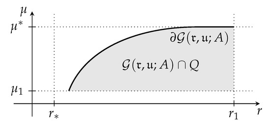  Figure 1. Illustration to show ${\mathcal{G}}_{\mathrm{eff}}(\mathfrak{r},\mathfrak{u};A)\ne \varnothing$.

This completes the proof. □

As indicated by the last theorem, the efficient frontier ${\mathcal{G}}_{\mathrm{eff}}(\mathfrak{r},\mathfrak{u};A)$ is not necessarily the whole boundary of $\mathcal{G}(\mathfrak{r},\mathfrak{u};A)$. As a consequence, ${\mathcal{G}}_{\mathrm{eff}}(\mathfrak{r},\mathfrak{u};A)$ might be bounded. The corresponding bounds are defined as follows.

Definition 13.

In the situation of Setting 1, assume that ${\mathcal{G}}_{\mathit{eff}}(\mathfrak{r},\mathfrak{u};A)$ is non-empty. Define the bounds for risk and utility of efficient elements by

$$\begin{array}{ccc}{r}_{min}:=\underset{(r,\mu )\in {\mathcal{G}}_{\mathit{eff}}(\mathfrak{r},\mathfrak{u};A)}{inf}\left\{r\right\},\hfill & \hfill & {\mu }_{min}:=\underset{(r,\mu )\in {\mathcal{G}}_{\mathit{eff}}(\mathfrak{r},\mathfrak{u};A)}{inf}\left\{\mu \right\},\hfill \end{array}$$

(34a)

$$\begin{array}{ccc}{r}_{max}:=\underset{(r,\mu )\in {\mathcal{G}}_{\mathit{eff}}(\mathfrak{r},\mathfrak{u};A)}{sup}\left\{r\right\},\hfill & \hfill & {\mu }_{max}:=\underset{(r,\mu )\in {\mathcal{G}}_{\mathit{eff}}(\mathfrak{r},\mathfrak{u};A)}{sup}\left\{\mu \right\},\hfill \end{array}$$

(34b)

respectively.

The following alternative representation is similar as the one in (Maier-Paape and Zhu 2018a, Proposition 9) for the one-period market (see also (Platen 2018, Lemma 2.4.10)).

Lemma 2 (Infima/Suprema of ${\mathcal{G}}_{\mathrm{eff}}(\mathfrak{r},\mathfrak{u};A)$).

Let Setting 1 be given and assume ${\mathcal{B}}_{\mathfrak{r},\mathfrak{u},A}(r,\mu )$ is compact for all $r,\mu \in \mathbb{R}$, so that by Theorem 2 (b) in particular ${\mathcal{G}}_{\mathit{eff}}(\mathfrak{r},\mathfrak{u};A)$ is non-empty. Then,

$$\begin{array}{cc}{r}_{min}\hfill & =\underset{x\in dom\left(\mathfrak{u}\right)\cap dom\left(\mathfrak{r}\right)}{inf}\left\{\mathfrak{r}\left(x\right)\right\}<\infty ,\hfill \\ {\mu }_{max}\hfill & =\underset{x\in dom\left(\mathfrak{u}\right)\cap dom\left(\mathfrak{r}\right)}{sup}\left\{\mathfrak{u}\left(x\right)\right\}>-\infty ,\hfill \end{array}$$

and, depending on $r_{min}$ and ${\mu }_{max}$, we have

$$\begin{array}{cc}{r}_{max}\hfill & =\left\{\begin{array}{cc}{\displaystyle \underset{x\in {\mathcal{B}}_{\mathfrak{u},A}\left({\mu }_{max}\right)}{min}\left\{\mathfrak{r}\left(x\right)\right\},}\hfill & \mathit{if}{\mu }_{max}<\infty \mathit{and}{\mathcal{B}}_{\mathfrak{u},A}\left({\mu }_{max}\right)\cap dom\left(\mathfrak{r}\right)\ne \varnothing ,\hfill \\ \infty ,\hfill & \mathit{otherwise}.\hfill \end{array}\right.\hfill \end{array}$$

$$\begin{array}{cc}{\mu }_{min}\hfill & =\left\{\begin{array}{cc}{\displaystyle \underset{x\in {\mathcal{B}}_{\mathfrak{r},A}\left(r_{min}\right)}{max}\left\{\mathfrak{u}\left(x\right)\right\},}\hfill & \mathit{if}{r}_{min}>-\infty \mathit{and}{\mathcal{B}}_{\mathfrak{r},A}\left(r_{min}\right)\cap dom\left(\mathfrak{u}\right)\ne \varnothing ,\hfill \\ -\infty ,\hfill & \mathit{otherwise},\hfill \end{array}\right.\hfill \end{array}$$

If ${\mathcal{B}}_{\mathfrak{r},A}\left(r\right)$ is compact for all $r\in \mathbb{R}$, then $r_{min}>-\infty$ and ${\mathcal{B}}_{\mathfrak{r},A}\left(r_{min}\right)\ne \varnothing$. If ${\mathcal{B}}_{\mathfrak{u},A}\left(\mu \right)$ is compact for all $\mu \in \mathbb{R}$, then ${\mu }_{max}<\infty$ and ${\mathcal{B}}_{\mathfrak{u},A}\left({\mu }_{max}\right)\ne \varnothing$.

Proof. 

We define $B:=dom\left(\mathfrak{u}\right)\cap dom\left(\mathfrak{r}\right)$. By assumption, $B\ne \varnothing$. Since the vertical part of ∂$\mathcal{G}(\mathfrak{r},\mathfrak{u};A)$, if it exists, does not change the infimum in r, we get

$$r_{min}=\underset{(r,\mu )\in {\mathcal{G}}_{\mathrm{eff}}(\mathfrak{r},\mathfrak{u};A)}{inf}\left\{r\right\}=\underset{(r,\mu )\in \partial \mathcal{G}(\mathfrak{r},\mathfrak{u};A)}{inf}\left\{r\right\}=\underset{(r,\mu )\in \mathcal{G}(\mathfrak{r},\mathfrak{u};A)}{inf}\left\{r\right\}=\underset{x\in B}{inf}\left\{\mathfrak{r}\left(x\right)\right\}<\infty .$$

(35)

Analogously, the horizontal part of ∂$\mathcal{G}(\mathfrak{r},\mathfrak{u};A)$, if it exists, does not change the supremum in $\mu$ and therefore

$${\mu }_{max}=\underset{(r,\mu )\in {\mathcal{G}}_{\mathrm{eff}}(\mathfrak{r},\mathfrak{u};A)}{sup}\left\{\mu \right\}=\underset{(r,\mu )\in \partial \mathcal{G}(\mathfrak{r},\mathfrak{u};A)}{sup}\left\{\mu \right\}=\underset{(r,\mu )\in \mathcal{G}(\mathfrak{r},\mathfrak{u};A)}{sup}\left\{\mu \right\}=\underset{x\in B}{sup}\left\{\mathfrak{u}\left(x\right)\right\}>-\infty .$$

(36)

We next show the properties of $r_{max}$ and ${\mu }_{min}$. Since the properties of ${\mu }_{min}$ can be shown similarly, we only show it for $r_{max}$.

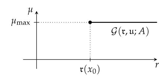
Firstly, assume that ${\mu }_{max}<\infty$ and ${\mathcal{B}}_{\mathfrak{u},A}\left({\mu }_{max}\right)\cap dom\left(\mathfrak{r}\right)\ne \varnothing$. Then, there exists $x_0\in {\mathcal{B}}_{\mathfrak{u},A}\left({\mu }_{max}\right)$ such that $\mathfrak{r}\left(x_0\right)\in \mathbb{R}$. Of course, $(\mathfrak{r}\left(x_0\right),\mathfrak{u}\left(x_0\right))=(\mathfrak{r}\left(x_0\right),{\mu }_{max})$ is on the horizontal part of ∂$\mathcal{G}(\mathfrak{r},\mathfrak{u};A)$, see Figure 2. By assumption, ${\mathcal{G}}_{\mathrm{eff}}(\mathfrak{r},\mathfrak{u};A)\ne \varnothing$ and hence the set $\{(r,{\mu }_{max}):r\in \mathbb{R}\}$ cannot be a subset of $\mathcal{G}(\mathfrak{r},\mathfrak{u};A)$. Therefore, and since $\mathcal{G}(\mathfrak{r},\mathfrak{u};A)$ is closed by Proposition 2 (d), we obtain $r_{*}:=min\{r:(r,{\mu }_{max})\in \mathcal{G}(\mathfrak{r},\mathfrak{u};A\left)\right\}>-\infty$. Using Equation (33), we get $(r_{*},{\mu }_{max})\in {\mathcal{G}}_{\mathrm{eff}}(\mathfrak{r},\mathfrak{u};A)$ yielding an efficient portfolio $x_1\in A$ with $(\mathfrak{r}\left(x_1\right),\mathfrak{u}\left(x_1\right))=(r_{*},{\mu }_{max})$. From Equation (34b), we conclude $r_{max}=r_{*}=min\{\mathfrak{r}\left(x\right):x\in {\mathcal{B}}_{\mathfrak{u},A}\left({\mu }_{max}\right)\}$ and the assertion is proved.

Figure 2. Illustration for the proof of Lemma 2.

Now, assume that ${\mu }_{max}=\infty$ or ${\mathcal{B}}_{\mathfrak{u},A}\left({\mu }_{max}\right)\cap dom\left(\mathfrak{r}\right)=\varnothing$. In both cases, the supremum ${\mu }_{max}$ of the $\mu$ values of ${\mathcal{G}}_{\mathrm{eff}}(\mathfrak{r},\mathfrak{u};A)$ is not attained in the risk utility space. Since $\mathcal{G}(\mathfrak{r},\mathfrak{u};A)$ is closed and convex by Proposition 2 (c) and (d), there cannot be a horizontal part of ∂$\mathcal{G}(\mathfrak{r},\mathfrak{u};A)$. In addition, ${\mathcal{G}}_{\mathrm{eff}}(\mathfrak{r},\mathfrak{u};A)\ne \varnothing$ by Theorem 2 (b) and because of Equation (33) there is a sequence ${\left[(r_n,{\mu }_n)\right]}_{n\in \mathbb{N}}\subset {\mathcal{G}}_{\mathrm{eff}}(\mathfrak{r},\mathfrak{u};A)$ such that ${\mu }_n\to {\mu }_{max}$ as $n\to \infty$, which is, w.l.o.g., strictly increasing in ${\mu }_n$. Then, this sequence must be strictly increasing in $r_n$ as well, otherwise, $(r_n,{\mu }_n)$ would not belong to an efficient element in A. If ${\mu }_{max}=\infty$, it then must be $r_{max}=\infty$ because $\mathcal{G}(\mathfrak{r},\mathfrak{u};A)$ is convex. If ${\mathcal{B}}_{\mathfrak{u},A}\left({\mu }_{max}\right)\cap dom\left(\mathfrak{r}\right)=\varnothing$ (and ${\mu }_{max}<\infty$) it must be $r_{max}=\infty$ as well, because otherwise, $(r,{\mu }_{max})\in \partial \mathcal{G}(\mathfrak{r},\mathfrak{u};A)$ for all $r>r_{max}$ but $(r,{\mu }_{max})\notin \mathcal{G}(\mathfrak{r},\mathfrak{u};A)$, which contradicts that $\mathcal{G}(\mathfrak{r},\mathfrak{u};A)$ is closed.

It remains to show the result in the special situation when ${\mathcal{B}}_{\mathfrak{r},A}\left(r\right)$ is compact for all $r\in \mathbb{R}$. Then, $\mathfrak{r}$ is lower semi-continuous (see, e.g., (Rockafellar 1972, Theorem 4.6 and 7.1)). Let $x^{\prime }\in dom\left(\mathfrak{r}\right)$ be arbitrary. Since ${\mathcal{B}}_{\mathfrak{r},A}\left(\mathfrak{r}\left(x^{\prime }\right)\right)$ is compact, the minimum of $\mathfrak{r}$ is attained in ${\mathcal{B}}_{\mathfrak{r},A}\left(\mathfrak{r}\left(x^{\prime }\right)\right)$ (see, e.g., (Barbu and Precupanu 2012, Theorem 2.8)).

The case when ${\mathcal{B}}_{\mathfrak{u},A}\left(\mu \right)$ is compact again can be shown similarly. □

Related to the bounds, we define next all relevant risk and utility levels of the efficient frontier.

Definition 14.

For Setting 1, we define the projection of ${\mathcal{G}}_{\mathit{eff}}(\mathfrak{r},\mathfrak{u};A)$ to the r- and μ-axis by

$$\begin{array}{cc}I\hfill & :=\left\{r\in \mathbb{R}:\exists \mu \in \mathbb{R}\mathrm{s}.\mathrm{t}.(r,\mu )\in {\mathcal{G}}_{\mathit{eff}}(\mathfrak{r},\mathfrak{u};A)\right\},\hfill \\ J\hfill & :=\left\{\mu \in \mathbb{R}:\exists r\in \mathbb{R}\mathrm{s}.\mathrm{t}.(r,\mu )\in {\mathcal{G}}_{\mathit{eff}}(\mathfrak{r},\mathfrak{u};A)\right\},\hfill \end{array}$$

respectively.

From Lemma 2, we already obtain the possibilities for the intervals I and J, see (Maier-Paape and Zhu 2018a, Corollary 2) for a related result in the one-period case.

Corollary 1.

In the situation of Lemma 2, we have $r_{min}=inf\left(I\right)$, $r_{max}=sup\left(I\right)$, ${\mu }_{min}=inf\left(J\right)$ and ${\mu }_{max}=sup\left(J\right)$. Furthermore, exactly one of the following situations holds true depending on the situation:

• $I=[r_{min},r_{max}]$ and $J=[{\mu }_{min},{\mu }_{max}]$;
• $I=[r_{min},\infty )$ and $J=[{\mu }_{min},{\mu }_{max})$, where ${\mu }_{max}=\infty$ is possible;
• $I=(r_{min},r_{max}]$ and $J=(-\infty ,{\mu }_{max}]$, where $r_{min}=-\infty$ is possible; or
• $I=(r_{min},\infty )$ and $J=(-\infty ,{\mu }_{max})$, where ${\mu }_{max}=\infty$ and/or $r_{min}=-\infty$ is possible.

In particular, I and J are non-empty intervals. Figure 3 shows some examples.

Figure 3. Illustration of efficient frontiers for different cases of the intervals I and J.

Proof. 

This is a direct consequence from Lemma 2. □

In Definition 14, we define all valid r and $\mu$ values (separated from each other and not the combinations of them) of the efficient frontier ${\mathcal{G}}_{\mathrm{eff}}(\mathfrak{r},\mathfrak{u};A)$, which must be on the boundary of $\mathcal{G}(\mathfrak{r},\mathfrak{u};A)$ according to Theorem 2. Within the valid r and $\mu$ area, this boundary is defined by the two functions

$$\begin{array}{cccc}\nu \hfill & :I\to \mathbb{R},\hfill & r\hfill & \mapsto \underset{(r,\mu )\in \mathcal{G}(\mathfrak{r},\mathfrak{u};A)}{sup}\left\{\mu \right\}=\underset{x\in {\mathcal{B}}_{\mathfrak{r},A}\left(r\right)}{sup}\left\{\mathfrak{u}\left(x\right)\right\},\hfill \end{array}$$

(37a)

$$\begin{array}{cccc}\gamma \hfill & :J\to \mathbb{R},\hfill & \mu \hfill & \mapsto \underset{(r,\mu )\in \mathcal{G}(\mathfrak{r},\mathfrak{u};A)}{inf}\left\{r\right\}=\underset{x\in {\mathcal{B}}_{\mathfrak{u},A}\left(\mu \right)}{inf}\left\{\mathfrak{r}\left(x\right)\right\},\hfill \end{array}$$

(37b)

where I and J are from Definition 14. Next, we show some important properties for both functions, see (Maier-Paape and Zhu 2018a, Proposition 8) for the one-period case and see also (Platen 2018, Proposition 2.4.15).

Proposition 3 (Functions related to efficient frontier).

In the situation of Setting 1, assume that ${\mathcal{B}}_{\mathfrak{r},\mathfrak{u},A}(r,\mu )$ is compact for all $r,\mu \in \mathbb{R}$. Then, the functions $\nu :I\to \mathbb{R}$ and $\gamma :J\to \mathbb{R}$ from Equation (37) are well-defined and continuous. Furthermore, we have

$$\begin{array}{c}\nu \left(r\right)=\underset{(r,\mu )\in \mathcal{G}(\mathfrak{r},\mathfrak{u};A)}{max}\left\{\mu \right\}=\underset{x\in {\mathcal{B}}_{\mathfrak{r},A}\left(r\right)}{max}\left\{\mathfrak{u}\left(x\right)\right\},\mathit{for}\mathit{all}r\in I,\hfill \end{array}$$

(38a)

$$\begin{array}{c}\gamma \left(\mu \right)=\underset{(r,\mu )\in \mathcal{G}(\mathfrak{r},\mathfrak{u};A)}{min}\left\{r\right\}=\underset{x\in {\mathcal{B}}_{\mathfrak{u},A}\left(\mu \right)}{min}\left\{\mathfrak{r}\left(x\right)\right\},\mathit{for}\mathit{all}\mu \in J,\hfill \end{array}$$

(38b)

while ν is increasing and concave and γ is increasing and convex.

Proof. 

We show only the properties of $\gamma$. The proof for $\nu$ can be done similarly.

Let $\mu \in J$ be arbitrary. From ${\mu }_{max}$ in Lemma 2 and Definition 14, we know that there must exist $x^{*}\in dom\left(\mathfrak{u}\right)\cap dom\left(\mathfrak{r}\right)$ (note that $dom\left(\mathfrak{u}\right)\cap dom\left(\mathfrak{r}\right)\ne \varnothing$) such that $\mu \le \mathfrak{u}\left(x^{*}\right)\le {\mu }_{max}$ and $r^{*}:=\mathfrak{r}\left(x^{*}\right)\in \mathbb{R}$. We then have $x^{*}\in {\mathcal{B}}_{\mathfrak{r},\mathfrak{u},A}(r^{*},\mu )\ne \varnothing$ and

$$\gamma \left(\mu \right)=\underset{(r,\mu )\in \mathcal{G}(\mathfrak{r},\mathfrak{u};A)}{inf}\left\{r\right\}=\underset{x\in {\mathcal{B}}_{\mathfrak{u},A}\left(\mu \right)}{inf}\left\{\mathfrak{r}\left(x\right)\right\}=\underset{x\in {\mathcal{B}}_{\mathfrak{r},\mathfrak{u},A}(r^{*},\mu )}{inf}\left\{\mathfrak{r}\left(x\right)\right\}.$$

(39)

The function $\mathfrak{r}$ restricted to the compact set ${\mathcal{B}}_{\mathfrak{r},\mathfrak{u},A}(r^{*},\mu )\subset dom\left(\mathfrak{r}\right)$ must have closed (even compact) sublevel sets and hence is lower semi-continuous on ${\mathcal{B}}_{\mathfrak{r},\mathfrak{u},A}(r^{*},\mu )$ (see (Rockafellar 1972, Theorem 7.1)). Consequently the infimum in Equation (39) becomes a minimum. Hence, Equation (38b) follows and $\gamma$ is well-defined. The function $\gamma$ is increasing which directly follows from the definition in Equation (37b) because ${\mathcal{B}}_{\mathfrak{u},A}\left({\mu }_1\right)\supset {\mathcal{B}}_{\mathfrak{u},A}\left({\mu }_2\right)$ for all ${\mu }_1<{\mu }_2$.

Obviously, $\left(\gamma \right(\mu ),\mu )\in \partial \mathcal{G}(\mathfrak{r},\mathfrak{u};A)$ for all $\mu \in J$. Hence, convexity of $\gamma$ follows from convexity of $\mathcal{G}(\mathfrak{r},\mathfrak{u};A)$. Then, we already know that $\gamma$ is continuous in the interior of the domain J (see (Rockafellar 1972, Theorem 10.1)). Closedness of $\mathcal{G}(\mathfrak{r},\mathfrak{u};A)$ (see Proposition 2 (d)), together with the possibilities for I and J (see Corollary 1), implies closedness of the epigraph of $\gamma$. Therefore, $\gamma$ must be lower semi-continuous (see (Rockafellar 1972, Theorem 7.1)). Since $\gamma$ is convex, it must even be continuous on J. □

An important consequence of the last result is the representation of ${\mathcal{G}}_{\mathrm{eff}}(\mathfrak{r},\mathfrak{u};A)$ as graph of $\nu$ and (after interchanging coordinates) of $\gamma$, see (Maier-Paape and Zhu 2018a, Theorem 4) for the one-period case and also (Platen 2018, Corollary 2.4.16).

Corollary 2 (Parametrization of efficient frontier as graph).

Let Setting 1 be given and assume that ${\mathcal{B}}_{\mathfrak{r},\mathfrak{u},A}(r,\mu )$ is compact for all $r,\mu \in \mathbb{R}$. Then, the efficient frontier has the representation

$${\mathcal{G}}_{\mathit{eff}}(\mathfrak{r},\mathfrak{u};A)=\{(r,\nu \left(r\right)):r\in I\}=\{(\gamma \left(\mu \right),\mu ):\mu \in J\}.$$

(40)

Moreover, ν and γ are strictly increasing and $\nu ={\gamma }^{-1}$, i.e., $\nu \left(\gamma \right(\mu \left)\right)=\mu$ for all $\mu \in J$ and $\gamma \left(\nu \right(r\left)\right)=r$ for all $r\in I$.

Proof. 

Theorem 2 (b) (see Equation (33)) and the definitions of I and J (see Definition 14) imply ${\mathcal{G}}_{\mathrm{eff}}(\mathfrak{r},\mathfrak{u};A)=\partial \mathcal{G}(\mathfrak{r},\mathfrak{u};A)\cap (I\times J)$. Because of Proposition 2 (c) together with Equation (33), there is exactly one element $(r^{*}\left(\mu \right),\mu )\in {\mathcal{G}}_{\mathrm{eff}}(\mathfrak{r},\mathfrak{u};A)$ for each fixed $\mu \in J$ and there is exactly one element $(r,{\mu }^{*}\left(r\right))\in {\mathcal{G}}_{\mathrm{eff}}(\mathfrak{r},\mathfrak{u};A)$ for each fixed $r\in I$. Obviously, it must be $r^{*}\left(\mu \right)=\gamma \left(\mu \right)$ and ${\mu }^{*}\left(r\right)=\nu \left(r\right)$. Uniqueness of the elements implies Equation (40).

Because of Equation (40) it directly follows that $\nu ={\gamma }^{-1}$. Hence, $\nu$ and $\gamma$ are bijective and, because of Proposition 3, increasing. Consequently, they must even be strictly increasing. □

This gives many reasonable results which we can use to show solvability of the two optimization problems in Equations (MinR) and (MaxU).

3.4. Efficient Portfolios

This final subsection links points on the efficient frontier to their corresponding portfolio/trading strategy. The first result gives the existence of solutions (see (Platen 2018, Theorem 2.4.19) for similar results). Note that from now on we formally “hide” the side condition $S_0^{\top }{v}_1\left(x\right)=\beta$ of Equations (MinR) and (MaxU) in the set A.

Theorem 3 (Existence for Problem 1).

Let Setting 1 and $\beta >0$ be given and assume $A\subset \{x\in {\mathbb{R}}^{M+1}:S_0^{\top }{v}_1\left(x\right)=\beta \}$ is non-empty and convex. Suppose ${\mathcal{B}}_{\mathfrak{r},\mathfrak{u},A}(r,\mu )$ is compact for all $r,\mu \in \mathbb{R}$ and let $I,J\subset \mathbb{R}$ be the intervals from Definition 14.

(a) 

For each $\mu \in J$, there exists an efficient element $x_{\mu }\in A$ with $\mathfrak{u}\left(x_{\mu }\right)=\mu$. The element $x_{\mu }$ also solves Equation (MinR).

(b) 

For each $r\in I$, there exists an efficient element $y_r\in A$ with $\mathfrak{r}\left(y_r\right)=r$. The element $y_r$ also solves Equation (MaxU).

(c) 

Each solution of Equation (MinR) for $\mu \in J$ and each solution of Equation (MaxU) for $r\in I$ is efficient. Moreover, each efficient element $x^{*}\in A$ solves Equation (MinR) for $\mu =\mathfrak{u}\left(x^{*}\right)$ and Equation (MaxU) for $r=\mathfrak{r}\left(x^{*}\right)$.

Proof. 

Statements (a) and (b) follow from Corollary 2. For instance, by Equation (40), for every $r\in I$, there exists some $y_r\in A$ with $\mathfrak{r}\left(y_r\right)=r$ and $\mathfrak{u}\left(y_r\right)=\nu \left(r\right)$. Clearly, $S_0^{\top }{v}_1\left(y_r\right)=\beta$ by assumption on A. Using Equation (38a), we conclude

$$\mathfrak{u}\left(y_r\right)=\nu \left(r\right)=\underset{x\in A}{max}\left\{\mathfrak{u}\left(x\right):\mathfrak{r}\left(x\right)\le r\right\}$$

yielding that $y_r$ solves Equation (MaxU) and, moreover, each efficient element $x^{*}\in A$ with risk value r solves Equation (MaxU) as well. Conversely, any (other) solution $y_r^{\prime }$ of Equation (MaxU) for $r\in I$ satisfies $\mathfrak{u}\left(y_r^{\prime }\right)=\nu \left(r\right)=\mathfrak{u}\left(y_r\right)$ and $\mathfrak{r}\left(y_r^{\prime }\right)\le r$. Since $y_r$ is efficient, $\mathfrak{r}\left(y_r^{\prime }\right)<r$ is not possible, i.e., we must have $\mathfrak{r}\left(y_r^{\prime }\right)=r$. Therefore, $y_r^{\prime }$ is efficient as well. The claim for $\mu \in J$ follows similarly. □

For uniqueness, more assumptions are required. If either $\mathfrak{u}$ is strictly concave or $\mathfrak{r}$ is strictly convex, the uniqueness is guaranteed, see (Maier-Paape and Zhu 2018a, Theorem 5) for the one-period case with finite probability space and also (Platen 2018, Theorem 2.4.20) for a similar result.

Theorem 4 (Uniqueness and efficient portfolio path).

Let the situation in Theorem 3 be given. Furthermore, assume that either $\mathfrak{u}$ is strictly concave in $dom\left(\mathfrak{u}\right)$ or $\mathfrak{r}$ is strictly convex in $dom\left(\mathfrak{r}\right)$. Then, the following holds.

(a) 

For each $\mu \in J$, there is exactly one efficient element $x_{\mu }\in A$ with $\mathfrak{u}\left(x_{\mu }\right)=\mu$, which in addition is the unique solution of Equation (MinR).

Furthermore, the mapping $\tilde{\gamma }:J\to A,\mu \mapsto x_{\mu }$ is continuous.

For each $\mu \notin J$ and $\mu \ge {\mu }_{max}=supJ$, there does not exist any solution of Equation (MinR).

If ${\mu }_{min}>-\infty$, then for $\mu \notin J$ and $\mu \le {\mu }_{min}$ (i.e., $\mu <{\mu }_{min}$, see Corollary 1) the solution of Equation (MinR) is not necessarily unique and can be an element in A which is not efficient.

(b) 

For each $r\in I$, there is exactly one efficient element $y_r\in A$ with $\mathfrak{r}\left(y_r\right)=r$, which in addition is the unique solution of Equation (MaxU).

Furthermore, the mapping $\tilde{\nu }:I\to A,r\mapsto y_r$ is continuous.

For each $r\notin I$ and $r\le r_{min}=infI$, there does not exist any solution of Equation (MaxU).

If $r_{max}<\infty$, then for $r\notin I$ and $r\ge r_{max}$ (i.e., $r>r_{max}$) the solution of Equation (MaxU) is not necessarily unique and can be an element in A, which is not efficient.

Proof. 

The existence of efficient elements is already guaranteed by Theorem 3. Let $(r^{*},{\mu }^{*})\in {\mathcal{G}}_{\mathrm{eff}}(\mathfrak{r},\mathfrak{u};A)$ be arbitrary. The uniqueness of an efficient element $x^{*}\in A$ with $(\mathfrak{r}\left(x^{*}\right),\mathfrak{u}\left(x^{*}\right))=(r^{*},{\mu }^{*})$ follows from strict convexity of $\mathfrak{r}$ or strict concavity of $\mathfrak{u}$, respectively, which we show next: Assume the solution $x^{*}$ is not unique. Then, there is an efficient element $x^{\prime }\in A$ with $x^{\prime }\ne x^{*}$ and $(\mathfrak{r}\left(x^{\prime }\right),\mathfrak{u}\left(x^{\prime }\right))=(r^{*},{\mu }^{*})=(\mathfrak{r}\left(x^{*}\right),\mathfrak{u}\left(x^{*}\right))$. For $x_0:=(x^{*}+x^{\prime })/2$ we have

$$\mathfrak{r}\left(x_0\right)\le \frac{1}{2}\mathfrak{r}\left(x^{*}\right)+\frac{1}{2}\mathfrak{r}\left(x^{\prime }\right)=r^{*}\mathrm{and}\mathfrak{u}\left(x_0\right)\ge \frac{1}{2}\mathfrak{u}\left(x^{*}\right)+\frac{1}{2}\mathfrak{u}\left(x^{\prime }\right)={\mu }^{*}.$$

(41)

Since either $\mathfrak{r}$ is strictly convex or $\mathfrak{u}$ is strictly concave, one of the two inequalities in Equation (41) must be strict, which contradicts $(r^{*},{\mu }^{*})\in {\mathcal{G}}_{\mathrm{eff}}(\mathfrak{r},\mathfrak{u};A)$. Hence, the efficient portfolio for $(r^{*},{\mu }^{*})\in {\mathcal{G}}_{\mathrm{eff}}(\mathfrak{r},\mathfrak{u};A)$ is unique.

Furthermore, $\tilde{\gamma }$ and $\tilde{\nu }$ are well-defined. Next, we show continuity. We only show this for $\tilde{\gamma }$ (continuity for $\tilde{\nu }$ can be shown similarly). Suppose $\tilde{\gamma }$ is discontinuous at some point ${\mu }_0\in J$. Then, there exist $c>0$ and a sequence ${\left({\mu }_n\right)}_{n\in \mathbb{N}}\subset J$ with ${\mu }_n\to {\mu }_0$ as $n\to \infty$ and $\parallel \tilde{\gamma }\left({\mu }_n\right)-\tilde{\gamma }\left({\mu }_0\right)\parallel \ge c$ for all $n\in \mathbb{N}$. Since $\gamma$ is continuous, see Proposition 3, we obtain that $(\mathfrak{r}\left(\tilde{\gamma }\left({\mu }_n\right)\right),\mathfrak{u}\left(\tilde{\gamma }\left({\mu }_n\right)\right))=(\gamma \left({\mu }_n\right),{\mu }_n)\to (\gamma \left({\mu }_0\right),{\mu }_0)$ as $n\to \infty$. Hence, for all $\epsilon >0$ there exists $n_0\left(\epsilon \right)\in \mathbb{N}$ such that $\tilde{\gamma }\left({\mu }_n\right)\in {\mathcal{B}}_{\mathfrak{r},\mathfrak{u},A}(\gamma \left({\mu }_0\right)+\epsilon ,{\mu }_0-\epsilon )$ for all $n\ge n_0\left(\epsilon \right)$. Since, e.g., ${\mathcal{B}}_{\mathfrak{r},\mathfrak{u},A}(\gamma \left({\mu }_0\right)+1,{\mu }_0-1)$ is compact, there exists a convergent subsequence of ${\left(\tilde{\gamma }\left({\mu }_n\right)\right)}_{n\in \mathbb{N}}$ with limit $x^{*}\in {\mathcal{B}}_{\mathfrak{r},\mathfrak{u},A}(\gamma \left({\mu }_0\right)+1,{\mu }_0-1)$. Using again lower semi-continuity of $\mathfrak{r}$ restricted to ${\mathcal{B}}_{\mathfrak{r},\mathfrak{u},A}(\gamma \left({\mu }_0\right)+1,{\mu }_0-1)$ and upper semi-continuity of $\mathfrak{u}$ restricted to ${\mathcal{B}}_{\mathfrak{r},\mathfrak{u},A}(\gamma \left({\mu }_0\right)+1,{\mu }_0-1)$ as in the proof of Proposition 2 (d) gives $x^{*}\in {\mathcal{B}}_{\mathfrak{r},\mathfrak{u},A}(\gamma \left({\mu }_0\right),{\mu }_0)$. Then, $x^{*}$ must be efficient, because $(\gamma \left({\mu }_0\right),{\mu }_0)\in {\mathcal{G}}_{\mathrm{eff}}(\mathfrak{r},\mathfrak{u};A)$, and we have $(\mathfrak{r}\left(x^{*}\right),\mathfrak{u}\left(x^{*}\right))=(\gamma \left({\mu }_0\right),{\mu }_0)$, i.e., $x^{*}=\tilde{\gamma }\left({\mu }_0\right)$. This is a contradiction, because it must be $\parallel x^{*}-\tilde{\gamma }\left({\mu }_0\right)\parallel \ge c>0$. Consequently, $\tilde{\gamma }$ is continuous.

The situations where $\mu \notin J$ or $r\notin I$ follow easily: For instance, in case $\mu \ge {\mu }_{max}$ and $\mu \notin J$, there is no portfolio $x\in A$ such that $\mathfrak{u}\left(x\right)\ge \mu$, see Equation (36). In the case $-\infty <\mu <{\mu }_{min}$, there is an efficient element (which also solves Equation (MinR)), namely $\tilde{\gamma }\left({\mu }_{min}\right)$, but there might also be a solution of Equation (MinR), e.g., $x^{\prime }\in A$, such that $\mathfrak{r}\left(x^{\prime }\right)=\mathfrak{r}\left(\tilde{\gamma }\left({\mu }_{min}\right)\right)$ and $\mu \le \mathfrak{u}\left(x^{\prime }\right)<\mathfrak{u}\left(\tilde{\gamma }\left({\mu }_{min}\right)\right)={\mu }_{min}$. However, this element $x^{\prime }$ is not efficient. □

Remark 8 

(Connection to (Maier-Paape and Zhu 2018a, Theorem 5)). In (Maier-Paape and Zhu 2018a, Theorem 5), a related result is shown for the one-period case $N=1$ for a finite probability space. The utility function therein is of the form $\mathfrak{u}\left(x\right)=E\left[u\left(S_1^{\top }x\right)\right]$, for some concave function $u:\mathbb{R}\to \mathbb{R}\cup \{-\infty \}$, and the risk function $\mathfrak{r}$ must be non-negative, convex and independent of $x^0$. Additional assumptions are that ${\mathcal{B}}_{\mathfrak{r},A}\left(r\right)$ is compact for all $r\in \mathbb{R}$ or ${\mathcal{B}}_{\mathfrak{u},A}\left(\mu \right)$ is compact for all $\mu \in \mathbb{R}$. This implies that ${\mathcal{B}}_{\mathfrak{r},\mathfrak{u},A}(r,\mu )$ is compact for all $r,\mu \in \mathbb{R}$ (cf. Proposition 2 (b)). Since (Maier-Paape and Zhu 2018a, Theorem 5) assumes moreover unit initial cost (i.e., $S_0^{\top }x=1$), this already gives all assumptions for Theorem 3 in the case that $v_1\left(x\right):=x$ for all $x\in A$.

However, the result in (Maier-Paape and Zhu 2018a, Theorem 5) is also a uniqueness result and therefore requires additional assumptions on $\mathfrak{u}$ and/or $\mathfrak{r}$. For this, either u must be strictly concave or $\mathfrak{r}$ must be strictly convex in the risky part (note that (c3) in (Maier-Paape and Zhu 2018a, Theorem 5) implies that ${\mathfrak{r}}^2$ is strictly convex in the risky part). (Maier-Paape and Zhu 2018a, Theorem 5) then gives uniqueness.

Since Theorems 3 and 4 with $v_1\left(x\right)=x$ are restricted to the set $A_{\beta }:=\{x\in {\mathbb{R}}^{M+1}:S_0^{\top }x=\beta \}$, e.g., for $\beta =1$, this additional assumption on $\mathfrak{r}$ (being strictly convex in the risky part) implies, that the function $\mathfrak{r}$ restricted to the set $A_{\beta }\cap A$ is strictly convex (and not only strictly convex on the risky part). Hence, the assumptions of (Maier-Paape and Zhu 2018a, Theorem 5) are stronger than the assumptions in Theorem 4 and give a similar result. Therefore, Theorem 4 is a full generalization of (Maier-Paape and Zhu 2018a, Theorem 5).

Note that the assumption in (Maier-Paape and Zhu 2018a, Theorem 5) that u is strictly concave, is not enough to obtain strict concavity of $\mathfrak{u}$ in the setting of (Maier-Paape and Zhu 2018a, Theorem 5). Hence, Assumption (c1) in (Maier-Paape and Zhu 2018a, Theorem 5) may not be enough to obtain uniqueness (other than falsely stated there). However, e.g., if S has no nontrivial risk-free portfolio, then $\mathfrak{u}\left(x\right)=E\left[u\left(S_1^{\top }x\right)\right]$ is strictly concave (see (Maier-Paape and Zhu 2018a, Proposition 6)), and uniqueness follows.

4. Application

Let us focus on Example 2 with the trading strategy generating function $v_{\mathrm{twr}}$ which ensures that the portfolio weights are constant after each time step. Our admissible set is given by

$$A_{\mathrm{twr}}=\left\{f\in {\mathbb{R}}^{M+1}:1+T_n^{\top }f>0\mathrm{a}.\mathrm{s}.\mathrm{for}n=1,\dots ,N\right\},$$

(42)

see Equation (22).

Looking at Problem 1 for some special risk and utility functions, we also need to ensure the second constraint. Using Equation (21), this constraint reads

$$S_0^{\top }{\left(v_{\mathrm{twr}}\right)}_1\left(f\right)={\mathcal{W}}_0\sum _{i=0}^M{f}_i=\beta .$$

The risk and utility functions we are looking at in the following are independent on ${\mathcal{W}}_0$. Hence, w.l.o.g., we may set ${\mathcal{W}}_0:=1$. The set of all vectors fulfilling the second constraint in Problem 1 is then given by

$$A_{\beta }:=\left\{f\in {\mathbb{R}}^{M+1}:S_0^{\top }{\left(v_{\mathrm{twr}}\right)}_1\left(f\right)=\beta \right\}=\left\{f\in {\mathbb{R}}^{M+1}:\sum _{i=0}^M{f}_i=\beta \right\}.$$

(43)

Lemma 3 (utility function; logarithm of TWR).

Let the multi-period market model S be given and assume that $T_n\in {\mathcal{L}}^1(\Omega ,{\mathcal{F}}_n,\mathrm{P};{\mathbb{R}}^{M+1})$ for $n=1,\dots ,N$, where $T_n$ is from Equation (19) in Example 2. Define ${\mathfrak{u}}_{\mathrm{logTWR}}$ as in Equation (28), i.e.,

$${\mathfrak{u}}_{\mathrm{logTWR}}\left(f\right)=E\left[ln\left(TWR\left(f\right)\right)\right]=\sum _{n=1}^{N}E\left[ln\left(1+T_n^{\top }f\right)\right]$$

(44)

for $f\in A_{\mathrm{twr}}$ and ${\mathfrak{u}}_{\mathrm{logTWR}}\left(f\right)=-\infty$ for all $f\notin A_{\mathrm{twr}}$.

Then, ${\mathfrak{u}}_{\mathrm{logTWR}}$ is proper concave and ${\mathfrak{u}}_{\mathrm{logTWR}}<\infty$. Furthermore, if S has no nontrivial risk-free trading strategy, then ${\mathfrak{u}}_{\mathrm{logTWR}}$ restricted to $dom\left({\mathfrak{u}}_{\mathrm{logTWR}}\right)\cap A_{\beta }$, with $A_{\beta }$ from Equation (43), is strictly concave and ${\mathcal{B}}_{{\mathfrak{u}}_{\mathrm{logTWR}},A_{\beta }}\left(\mu \right)$ is bounded for all $\mu \in \mathbb{R}$ and all $\beta >0$.

Proof. 

Since $ln(1+s)\le s$ for all $s>-1$ and $T_n$ has a finite expectation by assumption, we have for all $f\in A_{\mathrm{twr}}$ that

$${\mathfrak{u}}_{\mathrm{logTWR}}\left(f\right)=\sum _{n=1}^{N}E\left[ln\left(1+T_n^{\top }f\right)\right]\le \sum _{n=1}^{N}E{\left[T_n\right]}^{\top }f<\infty$$

(45)

Of course, we also have ${\mathfrak{u}}_{\mathrm{logTWR}}\left(f\right)=-\infty <\infty$ for all $f\notin A_{\mathrm{twr}}$.

The mapping $f\mapsto ln(1+T_n{\left(\omega \right)}^{\top }f)$ is concave for each $\omega \in \Omega$. Because of linearity and monotonicity of the expectation, the mapping $f\mapsto E[ln(1+T_n^{\top }f)]$ is concave. The same holds true for ${\mathfrak{u}}_{\mathrm{logTWR}}$. Obviously, $0\in dom\left({\mathfrak{u}}_{\mathrm{logTWR}}\right)$ because ${\mathfrak{u}}_{\mathrm{logTWR}}\left(0\right)=0$ and therefore we obtain that the function ${\mathfrak{u}}_{\mathrm{logTWR}}$ is proper concave.

Now, assume that S has no nontrivial risk-free trading strategy. Because of Theorem 1 (d), $\mathcal{W}$ is injective in the risky part. Using the definition of $v_{\mathrm{twr}}$ in Equation (21), we obtain that $\mathcal{W}\left(v_{\mathrm{twr}}\left(f\right)\right)=\mathcal{W}\left(v_{\mathrm{twr}}\left(f^{\prime }\right)\right)$ a.s. for $f,f^{\prime }\in A_{\beta }$ implies $\widehat{f}={\widehat{f}}^{\prime }$. Since $f,f^{\prime }\in A_{\beta }$, it even must be $f=f^{\prime }$ if $\mathcal{W}\left(v_{\mathrm{twr}}\left(f\right)\right)=\mathcal{W}\left(v_{\mathrm{twr}}\left(f^{\prime }\right)\right)$ a.s.

Consequently, for arbitrary $f,f^{\prime }\in dom\left({\mathfrak{u}}_{\mathrm{logTWR}}\right)\cap A_{\beta }$ with $f\ne f^{\prime }$ there exists $n\in \{1,\dots ,N\}$ such that $T_n^{\top }f\equiv T_n^{\top }{f}^{\prime }$, i.e., $T_n^{\top }f\ne T_n^{\top }{f}^{\prime }$ with positive probability (see Equation (20)). Therefore, for all $\lambda \in (0,1)$, we obtain from strict concavity of ln that

$$\mathrm{P}\left(ln\left(1+T_n^{\top }\left(\lambda f+(1-\lambda )f^{\prime }\right)\right)>\lambda ln\left(1+T_n^{\top }f\right)+(1-\lambda )ln\left(1+T_n^{\top }{f}^{\prime }\right)\right)>0.$$

It follows that

$$E\left[ln\left(1+T_n^{\top }\left(\lambda f+(1-\lambda )f^{\prime }\right)\right)\right]>E\left[\lambda ln\left(1+T_n^{\top }f\right)+(1-\lambda )ln\left(1+T_n^{\top }{f}^{\prime }\right)\right].$$

This implies strict concavity for at least one summand of ${\mathfrak{u}}_{\mathrm{logTWR}}$ which directly gives strict concavity of ${\mathfrak{u}}_{\mathrm{logTWR}}$ restricted to $dom\left({\mathfrak{u}}_{\mathrm{logTWR}}\right)\cap A_{\beta }$.

The boundedness of ${\mathcal{B}}_{{\mathfrak{u}}_{\mathrm{logTWR}},A_{\beta }}\left(\mu \right)\subset dom\left({\mathfrak{u}}_{\mathrm{logTWR}}\right)\cap A_{\beta }$ directly follows from Lemma 1, because $dom\left({\mathfrak{u}}_{\mathrm{logTWR}}\right)\cap A_{\beta }\subset A_{\mathrm{twr}}\cap A_{\beta }$ is admissible for the trading strategy generating function $v_{\mathrm{twr}}$ (see Definition 8 and Equation (20)) and the corresponding matrix $\mathbf{B}$ in Lemma 1 for this example is a diagonal matrix with positive entries $b_{ii}={\mathcal{W}}_0/S_0^i>0$, for $i=0,1,\dots ,M$, on the diagonal (see Equation (21)). □

Lemma 4 (risk function; logarithm of TWR).

As in Lemma 3, let the multi-period market model S be given and assume that $T_n\in {\mathcal{L}}^1(\Omega ,{\mathcal{F}}_n,\mathrm{P};{\mathbb{R}}^{M+1})$ for $n=1,\dots ,N$, where $T_n$ is from Equation (19) in Example 2. Define the log drawdown function ${\rho }_{\ln }$ (see Equation (31)), by

$${\rho }_{\ln }\left(f\right)=E\left[max\left\{0,\underset{1\le \ell \le N}{max}\left\{-ln\left({TWR}_{\ell }^N\left(f\right)\right)\right\}\right\}\right]=E\left[max\left\{0,\underset{1\le \ell \le N}{max}\left\{-\sum _{n=\ell }^{N}ln\left(1+T_n^{\top }f\right)\right\}\right\}\right],$$

for $f\in A_{\mathrm{twr}}$ and ${\rho }_{\ln }\left(f\right)=\infty$ for all $f\notin A_{\mathrm{twr}}$. Then, ${\rho }_{\ln }$ is proper convex, ${\rho }_{\ln }\ge 0$ and $dom\left({\rho }_{\ln }\right)=dom\left({\mathfrak{u}}_{\mathrm{logTWR}}\right)$. If S has no nontrivial risk-free trading strategy, then ${\mathcal{B}}_{{\rho }_{\ln },A_{\beta }}\left(r\right)$ is bounded for all $r\in \mathbb{R}$ and all $\beta >0$.

Proof. 

The property ${\rho }_{\ln }\ge 0$ is obvious. Since $f\mapsto -ln(1+T_n^{\top }f)$ is convex and the maximum of convex functions again is convex, it follows that ${\rho }_{\ln }$ is convex as well. In addition, ${\rho }_{\ln }\left(0\right)=0$ and therefore $0\in dom\left({\rho }_{\ln }\right)$. Hence, ${\rho }_{\ln }$ is proper convex.

Inserting the known characterizations of ${\mathfrak{u}}_{\mathrm{logTWR}}$ and ${\rho }_{\ln }$ from above and using the properties of the logarithm yield for $f\in A_{\mathrm{twr}}$ that

$$\begin{array}{cc}{\mathfrak{u}}_{\mathrm{logTWR}}\left(f\right)+{\rho }_{\ln }\left(f\right)\hfill & =E\left[\sum _{n=1}^{N}ln\left(1+T_n^{\top }f\right)+max\left\{0,\underset{1\le \ell \le N}{max}\left\{-\sum _{n=\ell }^{N}ln\left(1+T_n^{\top }f\right)\right\}\right\}\right]\hfill \\ \hfill & =E\left[max\left\{0,\underset{1\le \ell \le N}{max}\left\{\sum _{n=1}^{\ell }ln\left(1+T_n^{\top }f\right)\right\}\right\}\right]\hfill \\ \hfill & \le E\left[\sum _{n=1}^N{T}_n^{\top }f\right]<\infty ,\hfill \end{array}$$

because $T_n\in {\mathcal{L}}^1(\Omega ,{\mathcal{F}}_n,\mathrm{P};{\mathbb{R}}^{M+1})$. Of course, we directly see from this that we also have ${\mathfrak{u}}_{\mathrm{logTWR}}\left(f\right)+{\rho }_{\ln }\left(f\right)\ge 0$. Hence, whenever ${\mathfrak{u}}_{\mathrm{logTWR}}\left(f\right)\in \mathbb{R}$, it must be ${\rho }_{\ln }\left(f\right)\in \mathbb{R}$ and vice versa. It directly follows that $dom\left({\rho }_{\ln }\right)=dom\left({\mathfrak{u}}_{\mathrm{logTWR}}\right)$. As in the proof of Lemma 3, the boundedness of ${\mathcal{B}}_{{\rho }_{\ln },A_{\beta }}\left(r\right)\subset A_{\beta }$ directly follows from Lemma 1. □

It is worth noting that ${\rho }_{\ln }$ may not be strictly convex.

Remark 9 

(Connection to Maier-Paape and Zhu (2018b)). Maier-Paape and Zhu (2018b) proved properties such as convexity for risk functions involving the relative drawdown but for a one-period market model. The function ${\mathfrak{r}}_{\mathrm{cur}}$ discussed therein corresponds to ${\rho }_{\ln }$ from Lemma 4 in the case we have a finite and discrete market model where the rates of returns are iid.

Assume we want to solve an optimization such as Equation (MinR) or Equation (MaxU) using the utility and risk functions from Lemmas 3 and 4, respectively, and the corresponding trading strategy generating function $v_{\mathrm{twr}}$. All requirements for Setting 1 are then fulfilled (note that $0\in dom\left({\mathfrak{u}}_{\mathrm{logTWR}}\right)=dom\left({\rho }_{\ln }\right)\ne \varnothing$). To be able to apply Theorem 3 or Theorem 4, we need that ${\mathcal{B}}_{{\rho }_{\ln },{\mathfrak{u}}_{\mathrm{logTWR}},A_{\beta }}(r,\mu )$ is compact for all $r,\mu \in \mathbb{R}$. From Lemma 3, we obtain boundedness in case S has no nontrivial risk-free trading strategy. However, in general, it is not clear whether or not the superlevel sets of ${\mathfrak{u}}_{\mathrm{logTWR}}$ are closed. Moreover, we do not know whether $dom\left({\rho }_{\ln }\right)=A_{\mathrm{twr}}$ holds true. Before we discuss the solutions of the corresponding optimization problems in Equations (MinR) and (MaxU), we firstly need to take care of these assumptions. We start with a more specific situation where we can ensure the compactness of ${\mathcal{B}}_{{\rho }_{\ln },{\mathfrak{u}}_{\mathrm{logTWR}},A_{\beta }}(r,\mu )$.

Remark 10 (ρ_ln and u_logTWR in finite probability space).

Assume the probability space is finite, e.g., with $\Omega :=\{{\omega }_1,\dots ,{\omega }_K\}$ for some fixed $K\in \mathbb{N}$ and $p_k:=\left(\left\{{\omega }_k\right\}\right)>0$ for all $k=1,\dots ,K$. Then, $A_{\mathrm{twr}}$ in Equation (42) becomes

$$A_{\mathrm{twr}}=\left\{f\in {\mathbb{R}}^{M+1}:1+T_n{\left({\omega }_k\right)}^{\top }f>0\mathit{for}n=1,\dots ,N\mathit{and}k=1,\dots ,K\right\},$$

(46)

where $T_n\left({\omega }_k\right)\in {\mathbb{R}}^{M+1}$ for each $n=1,\dots ,N$ and $k=1,\dots ,K$ is a vector fixed for a given market (see Equation (19)). Clearly, $0\in A_{\mathrm{twr}}$. Furthermore, ${\mathfrak{u}}_{\mathrm{logTWR}}$ in Equation (44) becomes

$${\mathfrak{u}}_{\mathrm{logTWR}}\left(f\right)=\sum _{n=1}^N\left[\sum _{k=1}^K{p}_{k}ln\left(1+T_n{\left({\omega }_k\right)}^{\top }f\right)\right]$$

(47)

for $f\in A_{\mathrm{twr}}$. Then, we obviously get $dom\left({\mathfrak{u}}_{\mathrm{logTWR}}\right)=A_{\mathrm{twr}}$ because by definition ${\mathfrak{u}}_{\mathrm{logTWR}}{|}_{A_{\mathrm{twr}}^c}=-\infty$.

Now, let ${\left(f^m\right)}_{m\in \mathbb{N}}\subset A_{\mathrm{twr}}$ be a sequence such that $f^m\to f^{*}\in \partial A_{\mathrm{twr}}$ as $m\to \infty$. Then, there exist $n\in \{1,\dots ,N\}$ and $k\in \{1,\dots ,K\}$ such that $1+T_n{\left({\omega }_k\right)}^{\top }{f}^{*}=0$. In this case, we obtain ${\mathfrak{u}}_{\mathrm{logTWR}}\left(f^m\right)\to -\infty$ as $m\to \infty$. From this we, can conclude that $A_{\mathrm{twr}}$ is open and non-empty and, moreover, by Equation (47), ${\mathfrak{u}}_{\mathrm{logTWR}}{|}_{A_{\mathrm{twr}}}$ is continuous. In particular, the superlevel sets of ${\mathfrak{u}}_{\mathrm{logTWR}}$ are closed. Consequently, we also must have that ${\mathcal{B}}_{{\mathfrak{u}}_{\mathrm{logTWR}},A}\left(\mu \right)$ is closed for all closed sets A and all $\mu \in \mathbb{R}$.

Analogously, we obtain $dom\left({\rho }_{\ln }\right)=A_{\mathrm{twr}}=dom\left({\mathfrak{u}}_{\mathrm{logTWR}}\right)$ where the sublevel sets of ${\rho }_{\ln }$ and also ${\mathcal{B}}_{{\rho }_{\ln },A}\left(r\right)$ must be closed for all closed sets A and all $r\in \mathbb{R}$. Then, Proposition 2 (a) and Lemmas 3 and 4 yield that ${\mathfrak{u}}_{\mathrm{logTWR}}$ is closed proper concave and ${\rho }_{\ln }$ is closed proper convex.

In general, however, when $\Omega$ is not finite ${\mathfrak{u}}_{\mathrm{logTWR}}$ might not be closed proper concave and ${\rho }_{\ln }$ might not be closed proper convex. Since we assume these properties in the existence and uniqueness theorem (see Theorem 5 below), we make some more remarks to have a better understanding also in the general situation.

Remark 11 (Notes on $dom\left({\mathfrak{u}}_{\mathrm{logTWR}}\right)$ and $A_{\mathrm{twr}}$).

(a) 

Clearly $dom\left({\mathfrak{u}}_{\mathrm{logTWR}}\right)\subset A_{\mathrm{twr}}$.

(b) 

If $f\in A_{\mathrm{twr}}$, then, using Equation (20), it follows that ${\mathcal{W}}_n\left(v_{\mathrm{twr}}\left(f\right)\right)={\mathcal{W}}_0{\prod }_{k=1}^n(1+T_k^{\top }f)>0$ a.s. Of course, this is trivial and directly follows from the definition of $A_{\mathrm{twr}}$ in Equation (42). In fact, $A_{\mathrm{twr}}$ is defined as the admissible set of $v_{\mathrm{twr}}$ (see Example 2).

(c) 

We have

$$\begin{array}{cc}dom\left({\mathfrak{u}}_{\mathrm{logTWR}}\right)\hfill & =\left\{f\in {\mathbb{R}}^{M+1}:E\left[ln\left(1+T_n^{\top }f\right)\right]>-\infty \mathit{for}\mathit{all}n=1,\dots ,N\right\}\hfill \\ \hfill & =\left\{f\in {\mathbb{R}}^{M+1}:{\int }_{\Omega }ln\left(1+T_n{\left(\omega \right)}^{\top }f\right)d\mathrm{P}\left(\omega \right)>-\infty \mathit{for}\mathit{all}n=1,\dots ,N\right\}.\hfill \end{array}$$

Proof: The second equality holds by definition. For the first one, the relation “⊃” is obvious. Let now $f\in dom\left({\mathfrak{u}}_{\mathrm{logTWR}}\right)\subset A_{\mathrm{twr}}$ be arbitrary. Since ${\mathfrak{u}}_{\mathrm{logTWR}}\left(f\right)<\infty$ by Lemma 3 we have ${\mathfrak{u}}_{\mathrm{logTWR}}\left(f\right)\in \mathbb{R}$. In addition, $E[ln(1+T_n^{\top }f)]<\infty$ holds for $n=1,\dots ,N$ (cf. Equation (45)). Hence, it must be $E[ln(1+T_n^{\top }f)]>-\infty$ for $n=1,\dots ,N$, which shows the relation “⊂” and therefore the equality.

(d) 

Define

$$A_{\mathrm{twr}}^{*}:=\left\{f\in {\mathbb{R}}^{M+1}:\mathit{there}\mathit{exists}\epsilon >0\mathit{such}\mathit{that}1+T_n^{\top }f\ge \epsilon a.s.\mathit{for}\mathit{all}n=1,\dots ,N\right\}.$$

Then, we obtain $A_{\mathrm{twr}}^{*}\subset dom\left({\mathfrak{u}}_{\mathrm{logTWR}}\right)$.

Proof: Let $f\in A_{\mathrm{twr}}^{*}$ be arbitrary. Then, $ln(1+T_n^{\top }f)\ge ln\left(\epsilon \right)>-\infty$ a.s. This, of course, gives $E[ln(1+T_n^{\top }f)]\ge ln\left(\epsilon \right)>-\infty$.

Now, we can show the result for the optimization problems in Equations (MinR) and (MaxU) when using $\mathfrak{r}:={\rho }_{\ln }$ and $\mathfrak{u}:={\mathfrak{u}}_{\mathrm{logTWR}}$.

Theorem 5 (Existence and uniqueness for u_logTWR and ρ_ln).

Assume the multi-period market model S has no nontrivial risk-free trading strategy and $T_n\in {\mathcal{L}}^1(\Omega ,{\mathcal{F}}_n,\mathrm{P};{\mathbb{R}}^{M+1})$ for $n=1,\dots ,N$, where $T_n$ is from Equation (19) in Example 2. Let the trading strategy generating function be given by $v_{\mathrm{twr}}$ (constant weights) from Example 2, with admissible set $A_{\mathrm{twr}}$ as in Equation (42). Assume that ${\rho }_{\ln }$ and ${\mathfrak{u}}_{\mathrm{logTWR}}$ restricted to some convex and non-empty set $A\subset dom\left({\mathfrak{u}}_{\mathrm{logTWR}}\right)\cap A_{\beta }$ are closed proper convex and closed proper concave, respectively. We define the minimum log drawdown optimization problem for fixed $\mu \in \mathbb{R}$ by

$$\underset{f\in A}{min}{\rho }_{\ln }\left(f\right)\mathit{subject}\mathit{to}{\mathfrak{u}}_{\mathrm{logTWR}}\left(f\right)\ge \mu ,S_0^{\top }{\left(v_{\mathrm{twr}}\right)}_1\left(f\right)=\beta .$$

(MinDD)

We define the maximum log TWR optimization problem for fixed $r\in \mathbb{R}$ by

$$\underset{f\in A}{max}{\mathfrak{u}}_{\mathrm{logTWR}}\left(f\right)\mathit{subject}\mathit{to}{\rho }_{\ln }\left(f\right)\le r,S_0^{\top }{\left(v_{\mathrm{twr}}\right)}_1\left(f\right)=\beta .$$

(MaxTWR)

The following holds true:

(a) 

(Growth optimal trading strategy) The problem in Equation (MaxTWR) without risk restriction, i.e.,

$$\underset{f\in A}{max}{\mathfrak{u}}_{\mathrm{logTWR}}\left(f\right)\mathit{subject}\mathit{to}{S}_0^{\top }{\left(v_{\mathrm{twr}}\right)}_1\left(f\right)=\beta$$

(48)

has a unique solution $f_{max}^{*}\in A$. Moreover, we have ${\mu }_{max}={\mathfrak{u}}_{\mathrm{logTWR}}\left(f_{max}^{*}\right)\in \mathbb{R}$ and $r_{max}={\rho }_{\ln }\left(f_{max}^{*}\right)\in {\mathbb{R}}_{\ge 0}$, where ${\mu }_{max}$ and $r_{max}$ represent the suprema of ${\mathcal{G}}_{\mathit{eff}}(\mathfrak{r},\mathfrak{u};A)$ from Definition 13 for $\mathfrak{r}={\rho }_{\ln }$ and $\mathfrak{u}={\mathfrak{u}}_{\mathrm{logTWR}}$.

(b) 

(Risk minimal trading strategy) The problem in Equation (MinDD) without utility restriction, i.e.,

$$\underset{f\in A}{min}{\rho }_{\ln }\left(f\right)\mathit{subject}\mathit{to}{S}_0^{\top }{\left(v_{\mathrm{twr}}\right)}_1\left(f\right)=\beta ,$$

(49)

has a finite minimum risk value $r_{min}\in {\mathbb{R}}_{\ge 0}$. Furthermore, among all $f\in A$ which solve Equation (49), there is a unique element $f_{min}^{*}\in A$ with maximal ${\mathfrak{u}}_{\mathrm{logTWR}}$ value. In particular, $r_{min}={\rho }_{\ln }\left(f_{min}^{*}\right)\in {\mathbb{R}}_{\ge 0}$, but moreover ${\mu }_{min}={\mathfrak{u}}_{\mathrm{logTWR}}\left(f_{min}^{*}\right)\in \mathbb{R}$ hold true, where $r_{min}$ and ${\mu }_{min}$ represent the infima of ${\mathcal{G}}_{\mathit{eff}}(\mathfrak{r},\mathfrak{u};A)$ from Definition 13 for $\mathfrak{r}={\rho }_{\ln }$ and $\mathfrak{u}={\mathfrak{u}}_{\mathrm{logTWR}}$.

(c) 

For each $\mu \in J=[{\mu }_{min},{\mu }_{max}]\ne \varnothing$, there is exactly one efficient element $f_{\mu }^{*}\in A$ with ${\mathfrak{u}}_{\mathrm{logTWR}}\left(f_{\mu }^{*}\right)=\mu$, which is also the unique solution of Equation (MinDD). The mapping $\tilde{\gamma }:J\to A,\mu \mapsto f_{\mu }^{*}$ is continuous.

(d) 

For each $r\in I=[r_{min},r_{max}]\ne \varnothing$, there is exactly one efficient element ${\tilde{f}}_r^{*}\in A$ with ${\rho }_{\ln }\left({\tilde{f}}_r^{*}\right)=r$, which is also the unique solution of Equation (MaxTWR). The mapping $\tilde{\nu }:I\to A,\mu \mapsto {\tilde{f}}_{\mu }^{*}$ is continuous.

Proof. 

By assumption, ${\mathfrak{u}}_{\mathrm{logTWR}}$ and ${\rho }_{\ln }$, both restricted to A, are closed proper concave and closed proper convex, respectively. Using Lemma 3, we in addition obtain that ${\mathfrak{u}}_{\mathrm{logTWR}}$ is strictly concave in the set $A\subset dom\left({\mathfrak{u}}_{\mathrm{logTWR}}\right)\cap A_{\beta }$. Moreover, ${\mathcal{B}}_{{\mathfrak{u}}_{\mathrm{logTWR}},A}\left(\mu \right)={\mathcal{B}}_{{\mathfrak{u}}_{\mathrm{logTWR}},A_{\beta }}\left(\mu \right)\cap A$ is compact for all $\mu \in \mathbb{R}$ because of Lemma 3 and Proposition 2 (a). Analogously, ${\mathcal{B}}_{{\rho }_{\ln },A}\left(r\right)$ is compact for all $r\in \mathbb{R}$ because of Lemma 4 and Proposition 2 (a). Consequently, Proposition 2 (b) yields that ${\mathcal{B}}_{{\rho }_{\ln },{\mathfrak{u}}_{\mathrm{logTWR}},A}(r,\mu )$ is compact for all $r,\mu \in \mathbb{R}$. Theorem 4 can then be applied, which proves (c) and (d), if we can show that $I=[r_{min},r_{max}]$, $J=[{\mu }_{min},{\mu }_{max}]$. This is shown in the proofs of (a) and (b).

Proof of (a): Since ${\mathfrak{u}}_{\mathrm{logTWR}}$ is closed proper concave on A, we know that ${\mathfrak{u}}_{\mathrm{logTWR}}$ must be upper semi-continuous (cf. (Rockafellar 1972, Theorem 7.1)). In addition, ${\mathcal{B}}_{{\mathfrak{u}}_{\mathrm{logTWR}},A}\left(\mu \right)$ is compact and non-empty for some $\mu \in \mathbb{R}$. Hence, there must be a solution of Equation (48) (see (Barbu and Precupanu 2012, Theorem 2.8)). Uniqueness follows from strict concavity of ${\mathfrak{u}}_{\mathrm{logTWR}}$ restricted to $A\subset dom\left({\mathfrak{u}}_{\mathrm{logTWR}}\right)$. Furthermore, Lemma 2 yields that ${\mu }_{max}={\mathfrak{u}}_{\mathrm{logTWR}}\left(f_{max}^{*}\right)\in \mathbb{R}$ and, since $dom\left({\mathfrak{u}}_{\mathrm{logTWR}}\right)=dom\left({\rho }_{\ln }\right)$ by Lemma 4, that ${\mathfrak{r}}_{max}={\rho }_{\ln }\left(f_{max}^{*}\right)\in [0,\infty )$ (also by Lemma 2, note that ${\mathcal{B}}_{{\mathfrak{u}}_{\mathrm{logTWR}},A}\left({\mu }_{max}\right)$ contains only $f_{max}^{*}$).

Proof of (b): The function ${\rho }_{\ln }$ is closed proper convex on A by assumption and, hence, it is lower semi-continuous (cf. (Rockafellar 1972, Theorem 7.1)). In addition, ${\mathcal{B}}_{{\rho }_{\ln },A}\left(r\right)$ is compact and non-empty for some $r\in \mathbb{R}$. Then, there must be a solution of Equation (49) (see (Barbu and Precupanu 2012, Theorem 2.8)). Maximizing ${\mathfrak{u}}_{\mathrm{logTWR}}$ over all those solutions then, similar to in the proof of (a), gives a unique solution denoted by $f_{min}^{*}$. As above, Lemma 2 yields that $r_{min}={\rho }_{\ln }\left(f_{min}^{*}\right)\in [0,\infty )$. Since $dom\left({\mathfrak{u}}_{\mathrm{logTWR}}\right)=dom\left({\rho }_{\ln }\right)$, we get ${\mu }_{min}={\mathfrak{u}}_{\mathrm{logTWR}}\left(f_{min}^{*}\right)\in \mathbb{R}$. Altogether, we obtain that $I=[r_{min},r_{max}]$ and $J=[{\mu }_{min},{\mu }_{max}]$, which completes the proof. □

Note that $A_{\beta }\cap dom\left({\mathfrak{u}}_{\mathrm{logTWR}}\right)\ne \varnothing$ because obviously ${(\beta ,0,\dots ,0)}^{\top }\in A_{\beta }\cap dom\left({\mathfrak{u}}_{\mathrm{logTWR}}\right)$. Hence, there exists such a subset $A\subset A_{\beta }$ with the above required properties, e.g., $A=A_{\beta }\cap dom\left({\mathfrak{u}}_{\mathrm{logTWR}}\right)$. Furthermore, the “local” (closed) proper convexity of ${\rho }_{\ln }$ on A and the “local” (closed) proper concavity of ${\mathfrak{u}}_{\mathrm{logTWR}}$ on A, which are relevant according to Setting 1 (because of the domain of definition of both functions) and Theorem 5, can be provided for instance as follows by “global” assumptions.

Lemma 5.

In the situation of Lemma 3 and Lemma 4 assume that ${\rho }_{\ln }$ is closed proper convex and ${\mathfrak{u}}_{\mathrm{logTWR}}$ is closed proper concave. For $A_{\beta }$ from Equation (43) with fixed $\beta >0$ let $A^{\prime }\subset A_{\beta }$ be closed and convex such that $A:=A^{\prime }\cap dom\left({\mathfrak{u}}_{\mathrm{logTWR}}\right)$ is non-empty. Then, $A\subset dom\left({\mathfrak{u}}_{\mathrm{logTWR}}\right)\cap A_{\beta }$ is convex and non-empty. Furthermore, ${\rho }_{\ln }$ restricted to A is closed proper convex and ${\mathfrak{u}}_{\mathrm{logTWR}}$ restricted to A is closed proper concave.

Proof. 

First note that ${\mathfrak{u}}_{\mathrm{logTWR}}$ is closed proper concave and ${\rho }_{\ln }$ is closed proper convex but by definition both on ${\mathbb{R}}^{M+1}$. Of course, ${\mathfrak{u}}_{\mathrm{logTWR}}$ is proper concave and ${\rho }_{\ln }$ is proper convex on A as well. Since ${\mathcal{B}}_{{\mathfrak{u}}_{\mathrm{logTWR}},A}\left(\mu \right)=\{f\in A:{\mathfrak{u}}_{\mathrm{logTWR}}\left(f\right)\ge \mu \}\subset dom\left({\mathfrak{u}}_{\mathrm{logTWR}}\right)$ we can also write ${\mathcal{B}}_{{\mathfrak{u}}_{\mathrm{logTWR}},A}\left(\mu \right)=\{f\in {\mathbb{R}}^{M+1}:{\mathfrak{u}}_{\mathrm{logTWR}}\left(f\right)\ge \mu \}\cap A^{\prime }$. Hence, ${\mathcal{B}}_{{\mathfrak{u}}_{\mathrm{logTWR}},A}\left(\mu \right)$ must be closed because $\{f\in {\mathbb{R}}^{M+1}:{\mathfrak{u}}_{\mathrm{logTWR}}\left(f\right)\ge \mu \}$ is closed (cf. Proposition 2 (a) when replacing A by ${\mathbb{R}}^{M+1}$ therein) and $A^{\prime }$ is closed by assumption. Proposition 2 (a) then tells us that ${\mathfrak{u}}_{\mathrm{logTWR}}$ restricted to A is closed proper concave. A similar argumentation yields that ${\rho }_{\ln }$ restricted to A is closed proper convex. □

We have seen in Theorem 5 and Lemma 5 that one of the main ingredients to the existence and uniqueness theory for trading off risk and reward with ${\rho }_{\ln }$ and ${\mathfrak{u}}_{\mathrm{logTWR}}$ is that ${\rho }_{\ln }$ is closed proper convex and that ${\mathfrak{u}}_{\mathrm{logTWR}}$ is closed proper concave. While for finite probability space $\Omega$ this is already derived in Remark 10, in general this is not obvious. Lemma 4 and Lemma 3 just yield proper convex and proper concave, respectively. The following discussion closes this gap under reasonable conditions.

Lemma 6.

For $n\in \{1,\dots ,N\}$ fixed let $T_n\in {\mathcal{L}}^1(\Omega ,{\mathcal{F}}_n,\mathrm{P};{\mathbb{R}}^{M+1})$. Define

$$h_n\left(f\right):=\left\{\begin{array}{cc}E\left[ln\left(1+T_n^{\top }f\right)\right],\hfill & f\in D_n,\hfill \\ -\infty ,\hfill & f\notin D_n,\hfill \end{array}\right.$$

where $D_n:=dom\left(h_n\right)=\{f\in {\mathbb{R}}^{M+1}:E[ln(1+T_n^{\top }f)]>-\infty \}$. Assume that $0\in int\left(D_n\right)$, where $int\left(D_n\right)$ is the interior of $D_n$. Then, $h_n$ is closed proper concave.

Proof. 

Note that, according to Lemma 3, the function $h_n:{\mathbb{R}}^{M+1}\to \mathbb{R}\cup \{-\infty \}$ is proper concave and thus $D_n$ is convex. Therefore, $h_n$ is continuous in the interior of $D_n$ (cf. (Rockafellar 1972, Theorem 10.4)).

By assumption, $f_0:=0\in int\left(D_n\right)$ and $h_n\left(f_0\right)=ln\left(1\right)=0$. Using (Rockafellar 1972, Theorem 7.5), the closure of $h_n$ is of the form

$${\overline{h}}_n\left(f\right)=\underset{\lambda \nearrow 1}{lim}{h}_n\left((1-\lambda )f_0+\lambda f\right)=\underset{\lambda \nearrow 1}{lim}{h}_n\left(\lambda f\right),f\in {\mathbb{R}}^{M+1}.$$

(50)

The function ${\overline{h}}_n$ is known to be closed proper concave (see (Rockafellar 1972, Theorem 7.5.1)) with ${\overline{h}}_n\ge h_n$ and, moreover, ${\overline{h}}_n$ coincides with $h_n$ everywhere except possibly on $\partial D_n$ (see (Rockafellar 1972, Theorem 7.4)).

If we can show that ${\overline{h}}_n\left(f^{*}\right)=h_n\left(f^{*}\right)$ for all $f^{*}\in \partial D_n$, then ${\overline{h}}_n=h_n$ on ${\mathbb{R}}^{M+1}$ and thus $h_n$ is closed proper concave as well. To see that, we fix $f^{*}\in \partial D_n$ and set ${\lambda }_m:=1-1/m\nearrow 1$ (as $m\to \infty$). Since the limit in Equation (50) is independent of the sequence realizing $\lambda \nearrow 1$, we have

$${\overline{h}}_n\left(f^{*}\right)=\underset{m\to \infty }{lim}{h}_n\left({\lambda }_m{f}^{*}\right)\in \mathbb{R}\cup \{-\infty \}.$$

Define the random variables $Z_m^{+}:=max\{0,ln(1+T_n^{\top }{f}^{*}{\lambda }_m)\}$ and $Z_m^{-}:=min\{0,ln(1+T_n^{\top }{f}^{*}{\lambda }_m)\}$. By assumption, $T_n\in {\mathcal{L}}^1(\Omega ,{\mathcal{F}}_n,\mathrm{P};{\mathbb{R}}^{M+1})$ and, hence, as in Equation (45),

$$Z_m^{+}=max\left\{0,ln\left(1+T_n^{\top }{f}^{*}{\lambda }_m\right)\right\}\le max\left\{0,T_n^{\top }{f}^{*}{\lambda }_m\right\}\le max\left\{0,T_n^{\top }{f}^{*}\right\}.$$

Therefore, $0\le E\left[Z_m^{+}\right]\le E[max\{0,T_n^{\top }{f}^{*}\}]=:M_n<\infty$ which gives

$${\overline{h}}_n\left(f^{*}\right)=\underset{m\to \infty }{lim}E\left[ln\left(1+T_n^{\top }{f}^{*}{\lambda }_m\right)\right]=\underset{m\to \infty }{lim}E\left[Z_m^{-}\right]+\underset{m\to \infty }{lim}E\left[Z_m^{+}\right].$$

Since ln is increasing, $Z_m^{-}$ is monotonically decreasing in m (i.e., $Z_{m+1}^{-}\le Z_m^{-}\le 0$ a.s.) and $Z_m^{+}$ is monotonically increasing in m (i.e., $0\le Z_m^{+}\le Z_{m+1}^{+}$ a.s.). Hence, the monotone convergence theorem (see (Fristedt and Gray 1997, Section 8.2, Theorem 6)) implies

$${\overline{h}}_n\left(f^{*}\right)=E\left[\underset{m\to \infty }{lim}{Z}_m^{-}\right]+E\left[\underset{m\to \infty }{lim}{Z}_m^{+}\right]=E\left[ln\left(1+T_n^{\top }{f}^{*}\right)\right]=h_n\left(f^{*}\right),$$

(51)

which completes the proof. □

Note that in Equation (51) the limit might be finite (i.e., $f^{*}\in \partial D_n\cap D_n$) or $-\infty$ (i.e., $f^{*}\in \partial D_n\cap D_n^c$, where $D_n^c={\mathbb{R}}^{M+1}\setminus D_n$). In the latter case the transition of $h_n$ from $D_n$ to $D_n^c$ at the point $f^{*}$ is smooth, whereas in the first case $h_n$ jumps at $f^{*}$ (but still maintains upper semi-continuity). Both cases indeed occur as we show in Example 3 below.

Corollary 3.

Let S be a multi-period market model such that $T_n\in {\mathcal{L}}^1(\Omega ,{\mathcal{F}}_n,\mathrm{P};{\mathbb{R}}^{M+1})$ for $n=1,\dots ,N$, where $T_n$ is from Equation (19) in Example 2. Assume that $0\in int(dom\left({\mathfrak{u}}_{\mathrm{logTWR}}\right))$. Then, ${\rho }_{\ln }$ defined in Lemma 4 is closed proper convex and ${\mathfrak{u}}_{\mathrm{logTWR}}$ from Lemma 3 is closed proper concave.

Proof. 

Using Lemma 6, $h_n$ for $n=1,\dots ,N$ are closed proper concave and thus, in particular, upper semi-continuous (see (Rockafellar 1972, Theorem 7.1)). Hence, ${\mathfrak{u}}_{\mathrm{logTWR}}\left(f\right)={\sum }_{n=1}^N{h}_n\left(f\right)$, $f\in {\mathbb{R}}^{M+1}$, inherits these properties. The proof for ${\rho }_{\ln }$ is similar. □

We close this section with the already mentioned example.

Example 3 ($dom\left({\mathfrak{u}}_{\mathrm{logTWR}}\right)$, $A_{\mathrm{twr}}$ and $A_{\mathrm{twr}}^{*}$).

With Remark 11 (a) and (d), we already know that $A_{\mathrm{twr}}^{*}\subset dom\left({\mathfrak{u}}_{\mathrm{logTWR}}\right)\subset A_{\mathrm{twr}}$. We want to show at specific examples that $A_{\mathrm{twr}}^{*}⫋dom\left({\mathfrak{u}}_{\mathrm{logTWR}}\right)$ as well as $dom\left({\mathfrak{u}}_{\mathrm{logTWR}}\right)⫋A_{\mathrm{twr}}$ is possible. In all examples below we use $\omega =t\in (0,1)=:\Omega$ with $\mathrm{P}={\lambda }_{(0,1)}$ and $M=N=1$ and, for simplicity, we ignore the risk-free asset.

(a) 

Let $T_1\left(t\right):=exp(-1/t)-1\in (-1,0)$ for $t\in (0,1)$. Then

$${\mathfrak{u}}_{\mathrm{logTWR}}\left(f\right)=h_1\left(f\right)={\int }_0^{1}ln\left(1+T_1\left(t\right)f\right)dt,f\in dom\left(h_1\right)=dom\left({\mathfrak{u}}_{\mathrm{logTWR}}\right).$$

For $f\in (-\infty ,1)$, there exists some $M>0$ such that $1+T_1\left(t\right)f\ge M>0$ for all $t\in (0,1)$, but for $f\in (1,\infty )$ we have $1+T_1\left(t\right)f<0$ for t with positive measure. Hence, $A_{\mathrm{twr}}^{*}=(-\infty ,1)$ and $A_{\mathrm{twr}}=(-\infty ,1]$. Calculating

$$h_1\left(1\right)={\int }_0^{1}ln(1+T_1\left(t\right))dt={\int }_0^1-\frac{1}{t}dt=-\infty ,$$

we find $f^{*}:=1\notin dom\left(h_1\right)=dom\left({\mathfrak{u}}_{\mathrm{logTWR}}\right)=(-\infty ,1)$. In this example, we thus have $dom\left({\mathfrak{u}}_{\mathrm{logTWR}}\right)⫋A_{\mathrm{twr}}$. Moreover, since $0\in int(dom\left({\mathfrak{u}}_{\mathrm{logTWR}}\right))$, by Corollary 3, we obtain that ${\mathfrak{u}}_{\mathrm{logTWR}}$ is closed proper concave.

(b) 

Let ${\tilde{T}}_1\left(t\right):=exp(-1/\sqrt{t})-1\in (-1,0)$ for $t\in (0,1)$. Reasoning as in (a), we again get ${\tilde{A}}_{\mathrm{twr}}^{*}=(-\infty ,1)$ and ${\tilde{A}}_{\mathrm{twr}}=(-\infty ,1]$. However, this time

$${\tilde{h}}_1\left(1\right)={\int }_0^{1}ln(1+{\tilde{T}}_1\left(t\right))dt={\int }_0^1-\frac{1}{\sqrt{t}}dt=-2.$$

Hence, $f^{*}:=1\in dom\left({\tilde{h}}_1\right)=dom\left({\mathfrak{u}}_{\mathrm{logTWR}}\right)=(-\infty ,1]$ and therefore ${\tilde{A}}_{\mathrm{twr}}^{*}⫋dom\left({\mathfrak{u}}_{\mathrm{logTWR}}\right)$. Again ${\mathfrak{u}}_{\mathrm{logTWR}}$ is closed proper concave by Corollary 3.

5. Conclusions and Outlook

In this Part III of our series of papers on a general framework on the portfolio theory, we extend the results from Part I (Maier-Paape and Zhu 2018a) for the one-period financial market to a multi-period market model. We do so by using a modular approach that separates the framework into the four related modules: (a) multi-period market model; (b) trading strategy; (c) risk and utility function; and (d) optimization problem. This work provides an in itself complete general framework for handling the trade-off between competing performance criteria on reward and risk for trading strategies. This framework provides a foundation for implementation which is an interesting direction for further exploration.

Building Block (a) gives a lot of freedom for the market model. The most important assumption on the model should be that there is no nontrivial risk-free trading strategy. Block (b) gives the liberty for choosing a trading strategy. Even more complex trading strategies (besides the buy and hold strategy in Example 1 and fixed fraction strategy in Example 2) are possible, for instance the turtle trading strategy. This allows a more direct link between the portfolio theory and the real implementation of the optimal portfolios/trading strategies. Since Block (a) allows multi-period market models, the definition of the risk function (and also the utility function) in Block (c) can be path-dependent. This is essential for drawdown risk functions. Although so far we added lots of freedom, Block (d), i.e., the optimization block, is at least formally still very much in the spirit of Markowitz (1952, 1959). As such, this block is fixed in this work. However, different optimization problems might also be possible.

Clearly, with Parts I–III (see Maier-Paape and Zhu (2018a, 2018b)) we by now have a whole zoo of possibilities for how to trade off risk and reward in order to obtain efficient portfolios. Nevertheless, at this point, it is not yet clear what this added variety of possibilities yields when it comes to trading in real financial markets. This last and most important question will be discussed in a subsequent part of our series still to come.

References

- Barbu, Viorel, and Teodor Precupanu. 2012. Convexity and Optimization in Banach Spaces. Springer Monographs in Mathematics. Heidelberg: Springer. [Google Scholar]
- Carr, Peter, and Qiji Jim Zhu. 2018. Convex Duality and Financial Mathematics. Springer Briefs in Mathematics. Heidelberg: Springer. [Google Scholar]
- Chekhlov, Alexei, Stanislav Uryasev, and Michael Zabarankin. 2003. Portfolio optimization with drawdown constraints. In Asset and Liability Management Tools. London: Risk Books, pp. 263–78. [Google Scholar]
- Chekhlov, Alexei, Stanislav Uryasev, and Michael Zabarankin. 2005. Drawdown measure in portfolio optimization. International Journal of Theoretical and Applied Finance 8: 13–58. [Google Scholar] [CrossRef]
- Cherny, Vladimir, and Jan Obłój. 2013. Portfolio optimisation under non-linear drawdown constraints in a semimartingale financial model. Finance and Stochastics 17: 771–800. [Google Scholar] [CrossRef][Green Version]
- Cvitanić, Jaksa, and Ioannis Karatzas. 1995. On portfolio optimization under “drawdown” constraints. In Mathematical Finance. Volume 65 of The IMA Volumes in Mathematics and its Applications. Heidelberg: Springer. [Google Scholar]
- Fristedt, Bert E., and Lawrence F. Gray. 1997. A Modern Approach to Probability Theory. Basel: Birkhäuser. [Google Scholar]
- Föllmer, Hans, and Alexander Schied. 2016. Stochastic Finance: An Introduction in Discrete Time, 4th ed. Berlin: De Gruyter. [Google Scholar]
- Goldberg, Lisa R., and Ola Mahmoud. 2017. Drawdown: From practice to theory and back again. Mathematics and Financial Economics 11: 275–97. [Google Scholar] [CrossRef]
- Grossman, Sanford, and Zhongquan Zhou. 1993. Optimal investment strategies for controlling drawdowns. Mathematical Finance 3: 241–76. [Google Scholar] [CrossRef]
- Lintner, John. 1965. The valuation of risk assets and the selection of risky investments in stock portfolios and capital budgets. The Review of Economics and Statistics 47: 13–37. [Google Scholar] [CrossRef]
- Maier-Paape, Stanislaus, and Qiji Jim Zhu. 2018a. A general framework for portfolio theory. part I: Theory and various models. Risks 6: 53. [Google Scholar] [CrossRef]
- Maier-Paape, Stanislaus, and Qiji Jim Zhu. 2018b. A general framework for portfolio theory. part II: Drawdown risk measures. Risks 6: 76. [Google Scholar] [CrossRef]
- Markowitz, Harry. 1952. Portfolio selection. The Journal of Finance 7: 77–91. [Google Scholar]
- Markowitz, Harry. 1959. Portfolio Selection: Efficient Diversification of Investments. Number CFM 16. Hoboken: John Wiley & Sons. [Google Scholar]
- Mossin, Jan. 1966. Equilibrium in a capital asset market. Econometrica 34: 768–83. [Google Scholar] [CrossRef]
- Platen, Andreas. 2018. Modular Portfolio Theory: A General Framework with Risk and Utility Measures as well as Trading Strategies on Multi-Period Markets. Ph.D. thesis, RWTH Aachen, Aachen, Germany, November 21. [Google Scholar]
- Rockafellar, R. Tyrrell. 1972. Convex Analysis, 2nd ed. Princeton Landmarks in Mathematics and Physics. Princeton: Princeton University Press. [Google Scholar]
- Rockafellar, R. Tyrrell, Stan Uryasev, and Michael Zabarankin. 2006. Master funds in portfolio analysis with general deviation measures. Journal of Banking & Finance 30: 743–78. [Google Scholar] [CrossRef]
- Sharpe, William F. 1964. Capital asset prices: A theory of market equilibrium under conditions of risk. The Journal of Finance 19: 425–42. [Google Scholar] [CrossRef]
- Vince, Ralph. 2009. The Leverage Space Trading Model: Reconciling Portfolio Management Strategies and Economic Theory. Hoboken: John Wiley & Sons. [Google Scholar]
- Zabarankin, Michael, Konstantin Pavlikov, and Stan Uryasev. 2014. Capital asset pricing model (capm) with drawdown measure. European Journal of Operational Research 234: 508–17. [Google Scholar] [CrossRef]
© 2019 by the authors. Licensee MDPI, Basel, Switzerland. This article is an open access article distributed under the terms and conditions of the Creative Commons Attribution (CC BY) license (http://creativecommons.org/licenses/by/4.0/).