Direct and Hierarchical Models for Aggregating Spatially Dependent Catastrophe Risks

Abstract

We present several fast algorithms for computing the distribution of a sum of spatially dependent, discrete random variables to aggregate catastrophe risk. The algorithms are based on direct and hierarchical copula trees. Computing speed comes from the fact that loss aggregation at branching nodes is based on combination of fast approximation to brute-force convolution, arithmetization (regriding) and linear complexity of the method for computing the distribution of comonotonic sum of risks. We discuss the impact of tree topology on the second-order moments and tail statistics of the resulting distribution of the total risk. We test the performance of the presented models by accumulating ground-up loss for 29,000 risks affected by hurricane peril.

1. Introduction

The main objective of catastrophe (CAT) modeling is to predict the likelihood, severity and socio-economic consequences of catastrophic events such as hurricanes, earthquakes, pandemias and terrorism. Insurance companies use models to prepare for the financial impact from catastrophic events. Such models offer realistic loss estimates for a wide variety of future scenarios of catastrophes. Losses computed by CAT models can either be deterministic pertaining to a specific historical event (e.g., 2011 Tohoku earthquake in Japan or 2012 Hurricane Sandy in the U.S.), or probabilistic, inferred from an ensemble of hypothetical events (Clark 2015). In the probabilistic framework, large catalogs of events are randomly simulated using Monte-Carlo (MC) methods coupled with physical/conceptual models. For example, based on historical hurricane data, distributions of parameters such as frequencies, intensities, paths etc. are estimated and then used to randomly simulate values of these parameters to obtain a footprint of potential hurricane events in the period of, e.g., 10,000 catalog years. These events are not meant to predict hurricanes from year 2020 to year 12,020, but instead, each of the 10,000 years is considered as a feasible realization of the hurricane activity in the year 2020 (Latchman 2010).

Insurance companies investigate how catalog events affect a portfolio of properties using financial risk analysis (portfolio rollup). This operation typically consists of first aggregating event losses per property to obtain the event total loss, and then aggregating event totals within each catalog year to obtain the aggregate annual loss. Typically, the event loss per property, the event total, and the annual loss are all characterized by finite discrete probability distributions. Finally, the mixture of annual loss distributions is used to construct the exceedance probability (EP) curve Grossi et al. (2005). The EP curve is essentially the complementary cumulative distribution function which describes the portfolio loss, and is the key for insurers to estimate the probabilities of experiencing various levels of financial impact.

The first step of risk analysis for large insurance portfolio consists of probabilistic loss aggregation over a large number of locations for each event in the stochastic catalog. In the past few decades a number of methods have been proposed to address this difficult technical issue, see Shevchenko (2010); Wang (1998) for detailed overview. These approaches can roughly be categorized into three mainstream groups: (i) parametric, see e.g., Chaubey et al. (1998); Panjer and Lutek (1983); Venter (2001), where distributions characterizing individual losses belong to some parametric family and their convolution is given by an analytic expression or parametric closed form approximation, (ii) numerical, where individual loss distributions are given in discrete, generally non-parametric form and the distribution of the total risk is obtained using a variant of numerical convolution in Evans and Leemis (2004) boosted by Fast Fourier Transform in Robertson (1992) to make computations tractable (iii) MC, where, for a number of realizations, random samples are drawn from individual loss distributions and simply added up to obtain the aggregate loss, see e.g., Arbenz et al. (2012); Côté and Genest (2015); Galsserman (2004). The approach proposed in this paper originates from the category (ii). This is because of high computing speed requirement for ground-up/gross CAT loss analysis and also due to the fact that risks at different locations and their partial aggregates are described by discrete, generally non-parametric distributions (see Section 2.4 for details). We introduce two major enhancements to loss aggregation via numerical convolution. First, the proposed algorithm operates on irregular positive supports with the size of up to 300 points and treats atoms (point probability masses at minimum and maximum loss) separately. Second, positive correlations between pairs of risks are modeled by a mixture of Split-Atom convolution in Wojcik et al. (2016) and comonotonic distribution (Dhaene et al. 2002) of the sum of risks using several risk aggregation schemes based on copula trees in Arbenz et al. (2012); Côté and Genest (2015). High computing speed of our procedure stems from the fact that, by design, we aim at reproducing only the second order moments of the aggregate risk. Numerical experiments presented in this contribution show, however, that also tail measures of risk compare favorably with the estimates obtained from large sample MC runs.

The paper is organized as follows. First, we introduce the framework for aggregation of spatially dependent risks with copula trees and discuss direct and hierarchical models given positive dependence structure. Next, we present a computationally fast way to sum the dependent risks at branching nodes of a copula tree and algorithms for determining the tree topology. Finally, we show an example of ground-up loss estimation for a historical hurricane event in the U.S. Pros and cons of the proposed aggregation models are discussed and compared to the corresponding MC approach.

2. Copula Trees

2.1. Problem Statement

When aggregating CAT risks it is essential to account for spatial dependency between these risks relative to CAT model estimate. In general, combining dependent loss variables requires knowledge of their joint (multivariate) probability distribution. However, the available statistics describing the association between these variables are frequently limited to e.g., correlation matrix Wang (1998). To compute the aggregate loss distribution given such incomplete information, the risks are combined within copula trees (Arbenz et al. 2012; Côté and Genest 2015) where dependencies between losses are captured at each step of the aggregation using copula approach (see, e.g., Cherubini et al. 2004; Nelsen 2006). In the current study, we consider two accumulation schemes which assume non-negative correlations between pairs of risks. The question we attempt to answer is: “What is the most computationally efficient copula tree which aggregates spatially dependent risks pairwise and approximates non-parametric distribution of the sum of losses for a particular CAT event in such a way that its second order moments are reproduced?”

2.2. Direct Model

Following the idea in Wang (1998) and Dhaene et al. (2014) the positive dependence between risks can be represented using Fréchet copula via weighting independence and comonotonicity:

$$C_w(\mathbf{u})=(1-w)\prod _i{u}_i+wmin(\mathbf{u})0\le w\le 1,\forall \mathbf{u}$$

(1)

where $\mathbf{u}=[u_1,\dots ,u_M]\in {[0,1]}^M$. For portfolio of $M\ge 2$ risks $\mathbf{X}=[X_1,X_2,\dots X_M]$, assuming each $X_k$ has finite variance, let ${\mathbf{X}}^{\perp }=[X_1^{\perp },X_2^{\perp },\dots X_M^{\perp }]$ and ${\mathbf{X}}^{+}=[X_1^{+},X_2^{+},\dots X_M^{+}]$ be independent and comonotonic random vectors with the same marginals $P_{X_1},P_{X_2},\dots ,P_{X_M}$ as $\mathbf{X}$. By definition $P_{{\mathbf{X}}^{\perp }}(\mathbf{x})=\prod P_{X_i}(x_i)$ and $P_{{\mathbf{X}}^{+}}(\mathbf{x})=min(P_{X_1}(x_1),P_{X_2}(x_2),\dots ,P_{X_M}(x_M))$, which is equivalent to the statement that a random vector is either independent or comonotonic if and only if it has either product or min copula showed as the first and second summand in (1), respectively. For any positive dependent random vector $\mathbf{X}$ (Definition 2 and 3 in Koch and De Schepper 2011), (Collorary 2.3 in Koch and De Schepper 2006) the following bounds hold:

$$P_{\mathbf{X}}^{\perp }(\mathbf{x})\le P_{\mathbf{X}}(\mathbf{x})\le P_{\mathbf{X}}^{+}(\mathbf{x})\forall \mathbf{x}$$

(2)

Assuming that the distribution of $\mathbf{X}$ is induced by (1) and reads:

$$P_{\mathbf{X}}(\mathbf{x})=(1-w)P_{\mathbf{X}}^{\perp }(\mathbf{x})+w{P}_{\mathbf{X}}^{+}(\mathbf{x})0\le w\le 1,\forall \mathbf{x}$$

(3)

it follows from (Denuit et al. 2001, Theorem 3.1) and (Hürlimann 2001, Remark 2.1) that the dependent sum $S=X_1+X_2+\dots +X_M$ is always bounded in convex order by the corresponding independent sum $S^{\perp }=X_1^{\perp }+X_2^{\perp }+\dots +X_M^{\perp }$ and the comonotonic sum $S^{+}=X_1^{+}+X_2^{+}+\dots +X_M^{+}$. So,

$$S^{\perp }{\le }_{cx}S{\le }_{cx}{S}^{+}$$

(4)

where ${\le }_{cx}$ denotes the convex order. By definition

$$\mathrm{E}[v(S^{\perp })]\le \mathrm{E}[v(S)]\le \mathrm{E}[v(S^{+})]$$

(5)

for all real convex functions v, provided the expectations exist. As a consequence $S^{+}$ has heavier tails than S and the following variance order holds:

$$\mathrm{Var}[S^{\perp }]\le \mathrm{Var}[S]\le \mathrm{Var}[S^{+}]$$

(6)

In addition, $\mathrm{E}[S^{\perp }]=\mathrm{E}[S]=\mathrm{E}[S^{+}]$ since ${\mathbf{X}}^{\perp },\mathbf{X}$ and ${\mathbf{X}}^{+}$ belong to the same Fréchet class Dhaene et al. (2014). To approximate the distribution $P_S$ of the arbitrary sum S we use the weighted average

$$P_S(s)\approx (1-w)P_{S^{\perp }}(s)+w{P}_{S^{+}}(s)$$

(7)

where $P_{S^{\perp }}$ and $P_{S^{+}}$ are distributions of independent and comonotonic sums $S^{\perp }$ and $S^{+}$, respectively. Such ansatz, referred to as the the mixture method in Wang (1998), corresponds to the flat aggregation tree in the upper panel of Figure 1. For computational convenience, we elect to approximate the mixing coefficient w as the multivariate dependence measure in Dhaene et al. (2014), so

$$w=\frac{\mathrm{Var}(S)-\mathrm{Var}(S^{\perp })}{\mathrm{Var}(S^{+})-\mathrm{Var}(S^{\perp })}=\frac{{\sum }_{i\ne j}\mathrm{Cov}(X_i,X_j)}{{\sum }_{i\ne j}\mathrm{Cov}(X_i^{+},X_j^{+})}=\frac{{\sum }_{i\ne j}\mathrm{r}(X_i,X_j)}{{\sum }_{i\ne j}\mathrm{r}(X_i^{+},X_j^{+})}$$

(8)

where r is the classical Pearson correlation. Since the denominator of (8) is a normalizing constant which depends only on the shape of the marginals, any general correlation matrix $\mathrm{r}(X_i,X_j)={\rho }_{i,j}$ with positive entries as, e.g., shown in Figure 2B,C can be represented by the exchangeable correlation ${\rho }_e$ in Figure 2A without impacting the value of w. That is,

$${\rho }_e=\frac{{\sum }_{i\ne j}{\rho }_{i,j}}{M(M-1)}$$

(9)

Moreover, (8) is equivalent to the comonotonicity coefficient in Koch and De Schepper (2011) if (7) holds for all bivariate marginals:

$$P_{X_i,X_j}(x_i,x_j)=(1-w)P_{X_i^{\perp },X_j^{\perp }}(x_i,x_j)+w{P}_{X_i^{+},X_j^{+}}(x_i,x_j)$$

(10)

We observe that $w=\mathrm{r}(X_i,X_j)$ if and only if $\mathrm{r}(X_i^{+},X_j^{+})=1$ which holds when all univariate marginals differ only in location and/or scale parameters (Dhaene et al. 2002).

2.3. Hierarchical Model

If unique description of the joint distribution of individual risks is not crucial and the focus is solely on obtaining an easily interpretable model for the total risk, the individual risks can be aggregated in a hierarchical way. Such process involves specification of partial dependencies between the groups of risks in different aggregation steps (Arbenz et al. 2012). For pairwise accumulation, we first select the two risks $X_i,X_j$ and construct a copula model for that pair. Then, we replace $X_i$ and $X_j$ by their sum $X_i+X_j$ and treat it as a new, combined risk. A simple example is given in the middle panel of Figure 1 depicting the sequential risk aggregation scheme in Côté and Genest (2015). With bivariate (1) inducing the convex sum approximation (7) at the branching nodes we have:

$$\begin{array}{c}\hfill \begin{array}{cc}\hfill p_{S_1}=p_{X_1+X_2}& =(1-w_1)·p_{X_1^{\perp }+X_2^{\perp }}+w_1{p}_{X_1^{+}+X_2^{+}}\hfill \\ \hfill p_{S_2}& =(1-w_2)·p_{S_1^{\perp }+X_3^{\perp }}+w_2·p_{S_1^{+}+X_3^{+}}\hfill \\ \hfill ⋮& & \\ \hfill p_{S_4}& =(1-w_4)·p_{S_3^{\perp }+X_5^{\perp }}+w_4·p_{S_3^{+}+X_5^{+}}\hfill \end{array}\end{array}$$

(11)

For ease of notation, we dropped the arguments of the probability density functions (pdfs) characterizing the partial sums $S_i=X_1+\dots +X_{i+1}$. Observing that for the sequential tree, the partial sums $S_i^{\perp }$ and $S_i^{+}$ are symbolic abbreviations of ${(X_1+\dots +X_{i+1})}^{\perp }$ and ${(X_1+\dots +X_{i+1})}^{+}$ as opposed to $X_1^{\perp }+\dots +X_{i+1}^{\perp }$ and $X_1^{+}+\dots +X_{i+1}^{+}$ in (4), the partial weights $w_i$ read:

$$w_i=\frac{\mathrm{Var}[S_i]-\mathrm{Var}[S_i^{\perp }]}{\mathrm{Var}[S_i^{+}]-\mathrm{Var}[S_i^{\perp }]}$$

(12)

We remark, that if the order in which the aggregation is performed does not trivially follow from the tree structure, any convention can be used to make the numbering of partial sums unique, e.g., see Côté and Genest (2015). However, this has no implication on the fact that, in general, hierarchical trees do not uniquely determine the joint distribution of risk $\mathbf{X}$. To answer the research question posed in Section 2.1, this non-uniqueness is not critical. Conversely, in situations where, e.g., capital allocation is of interest (see Côté and Genest 2015), an extra conditional independence assumption in Arbenz et al. (2012) is needed. For instance, the aggregation scheme in the middle panel of Figure 1 would require:

$$\begin{array}{cc}\hfill (X_1,X_2,S_1)\perp (X_3,X_4,X_5,S_2,S_3,S_4)& |S_1\hfill \\ \hfill (X_1,X_2,X_3,S_1,S_2)\perp (X_4,X_5,S_3,S_4)& |S_2\hfill \\ \hfill (X_1,X_2,X_3,X_4,S_1,S_2,S_3)\perp (X_5,S_4)& |S_3\hfill \end{array}$$

(13)

2.4. Implementation of Risk Aggregation at Branching Nodes

A sample reordering method, inspired from Iman and Conover (1982) and assembled into the customized procedure in Arbenz et al. (2012), has recently been used to facilitate summation of risks in both the direct and hierarchical models. Despite the elegant simplicity of this approach, it comes at high computational cost for large samples. To reduce that cost and to orchestrate reproduction of the second order moments of the target sum S, we opt to use the following set of algorithms instead: (i) second order approximation to brute force convolution referred to as the Split-Atom convolution Wojcik et al. (2016), (ii) arithmetization (aka regriding) of loss distributions Vilar (2000), (iii) estimation of the distribution of the comonotonic sum of risks (comonotonization) and (iv) construction of the mixture distribution in (7). These algorithms are described in Section 2.4.1, Section 2.4.2 and Section 2.4.3. An individual risk X is a discrete random variable expressed in terms of the damage ratio defined as loss divided by replacement value. The corresponding pdf $p_X$ is represented by zero-and-one inflated mixture:

$$p_X(x)=\left\{\begin{array}{cc}\alpha ,\hfill & \mathrm{if}x=0\hfill \\ (1-\alpha -\beta ){\widehat{p}}_X(x),\hfill & \mathrm{if}0<x<1\hfill \\ \beta ,\hfill & \mathrm{if}x=1\hfill \end{array}\right.$$

(14)

where $\alpha$ and $\beta$ are atoms at zero and one damage ratio, respectively, and ${\widehat{p}}_X$ is the (discretized) pdf describing the main part of the mixture, see Figure 3 for an example and Section 3 for parameterization used in this study. The atoms are a common feature inferred from analysis of CAT insurance claims data. They also emerge during gross loss portfolio roll-up as a result of applying stop-loss insurance and/or re-insurance terms—deductibles and limits assembled into a variety of tiers/structures.

2.4.1. Split-Atom Convolution

The pdf $p_{S^{\perp }}$ of a sum of two independent discrete random variables X and Y with pdfs $p_X$ and $p_Y$ respectively, can be computed as:

$$p_{S^{\perp }}(s)=p_X\oplus p_Y=\sum _x{p}_X(x)p_Y(s-x)$$

(15)

The classical way of implementing (15) for random variables defined on irregular support is brute force (BF) convolution in Evans and Leemis (2004). Let $N_x$ and $N_y$ be the number of points discretizing $p_X$ and $p_Y$ support, respectively. The complexity of BF convolution is $O\left(N_x{N}_{y}log(N_x{N}_y)\right)$ because computing all possible products of probabilities and all possible sums of losses is $O(N_x{N}_y)$, and redundancy removal is $O(N_x{N}_{y}log(N_x{N}_y))$, see Evans and Leemis (2004) for details. Such high computational demand makes the BF algorithm impractical for convolving large number of CAT loss distributions. Our solution in Wojcik et al. (2016), referred to as the Split-Atom convolution, reduces the computational cost to $O(N_x^{\prime }{N}_y^{\prime })$ where $N_x^{\prime }<N_x$ and/or $N_y^{\prime }<N_y$. The idea is to separate two atoms (“spikes”) at min/max losses and arithmetize (regrid) the main parts of loss distributions. The regriding is the key to accelerating computations. The Split-Atom approach preserves min/max losses from different loss perspective (e.g., insurer, re-insurer, insured, FAC underwriter etc.) and enhances the accuracy of $p_S$ reproduction in situations where substantial probability mass is concentrated in the atoms. This is relevant for ground-up and, even more so, for gross loss estimation when stop-loss insurance is applied. Various ways of splitting the atoms and compacting main parts of loss distributions can be considered depending on computing speed and memory requirements and organization/arrangement of the original and convolution grids. An example is given in Algorithm 1. The original grids are non-uniform: the main parts of $p_X$ and $p_Y$ are defined on regular grids with spans $h_x$ and $h_y$, but the spacing between atoms and the main parts is arbitrary. Convolution grid is designed to have the same irregular spacing for preserving min/max losses. The speedup comes from execution of step 28 in Algorithm 1 using Algorithm 2. Depending on the application, other variants of the Split-Atom convolution are conceivable. For example, the 9-products approach in Algorithm 1 not only reproduces min/max losses but also probabilities describing these losses, or the 4-products approach which only splits the right atom to gain extra computing speed. See Appendix A, Algorithm A1.

Algorithm 1: Split-Atom Convolution: 9-products

Input: Two discrete pdfs $p_X$ and $p_Y$ with supports:    $x=\{x_1,x_2,x_2+h_x,x_2+2h_x,\dots ,x_2+(N_x-3)h_x,x_{N_x}\}$;    $y=\{y_1,y_2,y_2+h_y,y_2+2h_y,\dots ,y_2+(N_y-3)h_y,y_{N_y}\}$;    and probabilities: $p_X(x)={\sum }_{i=1}^{N_x}\delta (x-x_i)p_X(x_i)$; $p_Y(y)={\sum }_{i=1}^{N_y}\delta (y-y_i)p_Y(y_i)$    $N_s$ - maximum number of points for discretizing convolution grid   1: $x^{(1)}=\{x_1\}$; $p_X^{(1)}(x)=\delta (x-x^{(1)})p_X(x_1)$// split the left atom of $p_X$   2: $x^{(2)}=\{x_{N_x}\}$; $p_X^{(2)}(x)=\delta (x-x_i^{(2)})·p_X^{(2)}(x_i^{(2)})$// split the right atom of $p_X$   3: $x^{(3)}=\{x_2,x_2+h_x,x_2+2h_x,\dots ,x_2+(N_x-3)h_x\}$; $p_X^{(3)}(x)={\sum }_{i=1}^{N_x-2}\delta (x-x_i^{(3)})p_X^{(3)}(x_i^{(3)})$   4: $y^{(1)}=\{y_1\}$; $p_Y^{(1)}(y)=\delta (y-y^{(1)})p_Y(y_1)$// split the left atom of $p_Y$   5: $y^{(2)}=\{y_{N_y}\}$; $p_Y^{(2)}(y)=\delta (y-y_i^{(2)})·p_Y^{(2)}(y_i^{(2)})$// split the right atom of $p_Y$   6: $y^{(3)}=\{y_2,y_2+h_y,x_2+2h_y,\dots ,y_2+(N_y-3)h_y\}$; $p_Y^{(3)}(y)={\sum }_{i=1}^{N_y-2}\delta (y-y_i^{(3)})p_Y^{(3)}(y_i^{(3)})$   7: $h_{s^{★}}=\frac{x_{N_x}+y_{N_y}-(x_1+y_1)}{N_{s^{★}}-1}$// corresponding step size of the main part of convolution grid s    8: $h_s=max(h_x,h_y,h_{s^{★}})$// final step size of the main part of convolution grid s    9: $N_s=\lfloor \frac{x_{N_x}+y_{N_y}-(x_1+y_1)}{h_s}\rfloor$// corresponding number of points   10: // set irregular convolution grid:  11: if$h_s\ge (x_2+y_2-x_1-y_1)$then  12:  $s=\{x_1+y_1,x_2+y_2,x_2+y_2+h_s,\dots ,x_2+y_2+(N_s-3)h_s,x_{N_x}+y_{N_y}\}$  13: else  14:  $s=\{x_1+y_1,x_2+y_2-h_s,x_2+y_2,\dots ,x_2+y_2+(N_s-4)h_s,x_{N_x}+y_{N_y}\}$  15: end if  16: $x^{{(3)}^{\prime }}=\{x_2,x_2+h_s,x_2+2h_s,\dots ,x_2+(N_x-3)h_s\}$// discretize $x^{(3)}$ with $h_s$   17: $p_X^{{(3)}^{\prime }}(x)={\sum }_{i=1}^{N_x^{\prime }}\delta (x-x_i^{{(3)}^{\prime }})p_X^{{(3)}^{\prime }}(x_i^{{(3)}^{\prime }})$// regrid $p_X^{(3)}$   18: $y^{{(3)}^{\prime }}=\{y_2,y_2+h_s,y_2+2h_s,\dots ,y_2+(N_y-3)h_s\}$// discretize $y^{(3)}$ with $h_s$   19: $p_Y^{{(3)}^{\prime }}(y)={\sum }_{i=1}^{N_y^{\prime }}\delta (y-y_i^{{(3)}^{\prime }})p_Y^{{(3)}^{\prime }}(y_i^{{(3)}^{\prime }})$// regrid $p_Y^{(3)}$   20: ${\mathcal{B}}^{(1)}=p_X^{(1)}\oplus p_Y^{(1)}$// Brute Force convolution   21: ${\mathcal{B}}^{(2)}=p_X^{(2)}\oplus p_Y^{(1)}$// —”—   22: ${\mathcal{B}}^{(3)}=p_X^{{(3)}^{\prime }}\oplus p_Y^{(1)}$// —”—   23: ${\mathcal{B}}^{(4)}=p_X^{(1)}\oplus p_Y^{(2)}$// —”—   24: ${\mathcal{B}}^{(5)}=p_X^{(2)}\oplus p_Y^{(2)}$// —”—   25: ${\mathcal{B}}^{(6)}=p_X^{{(3)}^{\prime }}\oplus p_Y^{(2)}$// —”—   26: ${\mathcal{B}}^{(7)}=p_X^{(1)}\oplus p_Y^{{(3)}^{\prime }}$// —”—   27: ${\mathcal{B}}^{(8)}=p_X^{(2)}\oplus p_Y^{{(3)}^{\prime }}$// —”—   28: ${\mathcal{B}}^{(9)}=p_X^{{(3)}^{\prime }}\oplus p_X^{{(3)}^{\prime }}$// —”—   29: Regrid ${\mathcal{B}}^{(1-9)}$ onto convolution grid s Output: Discrete probability density function $p_{S^{\perp }}$ of the independent sum $S^{\perp }=X+Y$ with the support     $s=\{s_1,s_2,s_2+h_s,s_2+2h_s,\dots ,s_2+(N_s-3)h_s,s_{N_s}\}$ and the associated probabilities     $p_{S^{\perp }}(s)={\sum }_{k=1}^{N_s}\delta (s-s_k)p_{S^{\perp }}(s_k)$, where $s_{N_s}-[s_2+(N_s-3)h_s]\le h_s$, $s_2-s_1\le h_s$,     $h_s\ge max(h_1,h_2)$.

Algorithm 2: Brute force convolution for supports with the same span

Input: Two discrete probability density functions $p_X$ and $p_Y$, where the supports of X and Y are    defined using the same span h as: $x=\{x_1,x_1+h,\dots ,x_1+(N_x-1)h\}$,    $y=\{y_1,y_1+h,\dots ,y_1+(N_y-1)h\}$ and the associated probabilities as    $p_X(x)={\sum }_{i=1}^{N_x}\delta (x-x_i)p_X(x_i)$, $p_Y(y)={\sum }_{j=1}^{N_y}\delta (y-y_i)p_Y(y_j)$ 1: $s=\{x_1+y_1,x_1+y_1+h,x_1+y_1+2h,\dots ,x_1+y_1+(N_x+N_y-2)h\}$// compute convolution support 2: $p_{S^{\perp }}(s)=\mathbf{0}$// initialize 3: $p_{S^{\perp }}(s_{i+j-1})\leftarrow p_{S^{\perp }}(s_{i+j-1})+p_X(x_i)p_Y(y_j)1\le i\le N_x,1\le j\le N_y$// compute probabilities Output: Discrete probability density function $p_{S^{\perp }}$ of the independent sum $S^{\perp }=X+Y$ with the support     $s=\{s_1,s_2,\dots ,s_{N_x+N_y-1}\}$ and the corresponding probabilities     $p_{S^{\perp }}(s)={\sum }_{k=1}^{N_x+N_y-1}\delta (s_k)p_{S^{\perp }}(s_k)$.

Further acceleration of Algorithm 1 can be achieved using Fast Fourier Transform (FFT) and applying convolution theorem, (Wang 1998, Section 3.3.1) to convolve the main parts of $p_X$ and $p_Y$. Therefore, step 28 in Algorithm 1, is replaced with the following product:

$$p_X^{{(3)}^{\prime }}\oplus p_Y^{{(3)}^{\prime }}\stackrel{FFT}{\to }{P}_{{\Omega }_X}^{{(3)}^{\prime }}{P}_{{\Omega }_Y}^{{(3)}^{\prime }}\stackrel{IFFT}{\to }{p}_{X+Y}^{{(3,3)}^{\prime }}\to {\mathcal{B}}^{(9)}$$

(16)

where $P_{{\Omega }_1}^{{(3)}^{\prime }}$ and $P_{{\Omega }_2}^{{(3)}^{\prime }}$ represent FFTs of the probabilities $p_X^{{(3)}^{\prime }}$ and $p_Y^{{(3)}^{\prime }}$. IFFT in (16) stands for the Inverse Fast Fourier Transform. Implementation of (16) requires the supports $x^{{(3)}^{\prime }}$ and $y^{{(3)}^{\prime }}$ have the same span $h_s$, which is guaranteed by steps 16 and 18 in Algorithm 1, and also have the same range containing power-of-2 numbers of points, which can be guaranteed by extending one or both supports and padding zero probabilities.

2.4.2. Regriding

Split-Atom convolution requires that two pdfs being convolved have the main part of their supports discretized using the common span (grid step size) $h_s$, see step 8 in Algorithm 1. Prior to convolution, either one or both of these pdfs may need arithmetization hereafter referred to as the regriding. In general, this operation takes the discrete pdf $p_X$ defined on fine scale support with the span h and determines the new arithmetic pdf $p_{X^{\prime }}$ on coarse scale support with the span $h^{\prime }>h$ with the property ${\sum }_x{x}^m{p}_X(x)={\sum }_{x^{\prime }}{x^{\prime }}^m{p}_{X^{\prime }}(x^{\prime })$ of equating m moments with $p_X$ (see, e.g., Gerber 1982; Vilar 2000; Walhin and Paris 1998).

For $m=1$, linear regriding or mass dispersal in Gerber (1982) redistributes a probability mass on the original grid to two neighboring points on the new grid such that only $\mathrm{E}[X]$ is preserved. This is achieved by solving a $2\times 2$ local linear system, see Algorithm 3, Step 6 and animation therein. For $m=2$, the standard approach is to apply the method of local moment matching (LMM) which reproduces local second order moments of $p_X$ in predefined intervals on the new grid, assuring preservation of both $\mathrm{E}[X]$ and $\mathrm{Var}[X]$(Gerber 1982; Vilar 2000; Walhin and Paris 1998). Despite technical simplicity of LMM, there are two caveats: “wiggly” behavior and/or negative probabilities in $p_{X^{\prime }}$ (see, e.g., Table 4 in Walhin and Paris 1998). The first one is due to the fact that LMM performs local moment matching in fixed intervals $(x_k,x_k+2h^{\prime }],(x_k+2h^{\prime },x_k+4h^{\prime }],(x_k+4h^{\prime },x_k+6h^{\prime }]\dots$, etc. but ignores matching the moments in $(x_k+h^{\prime },x_k+3h^{\prime }],(x_k+3h^{\prime },x_k+5h^{\prime }],(x_k+5h^{\prime },x_k+7h^{\prime }]\dots ,$ etc. A simple improvement is proposed in Appendix A, Algorithm A2. The second caveat is that solving the 3 × 3 local linear system for matching the local moments (Equation (16) in Gerber 1982) guarantees a negative in the three dispersed probability masses. The negative mass can only be balanced out by a positive one dispersed from solving the next local linear system if the positive mass is greater than the negative one. Upon completion of the LMM algorithm, negative probabilities could still exist at arbitrary locations on the new grid. One way to handle this issue is to retreat to linear regriding as in Panjer and Lutek (1983). Another way is to use linear goal programming in Vilar (2000), i.e., for every span $h^{\prime }$ determine the arithmetic pdf which conserves the first moment $\mathrm{E}[X]$ and has the nearest second moment to the target $\mathrm{Var}[X]$. Therefore, the negative mass is mitigated by sacrificing the quality of reproducing $\mathrm{Var}[X]$. Here, we propose an alternative two-stage strategy listed in Algorithms 4 and 5 hereafter referred to as the 4-point regriding.

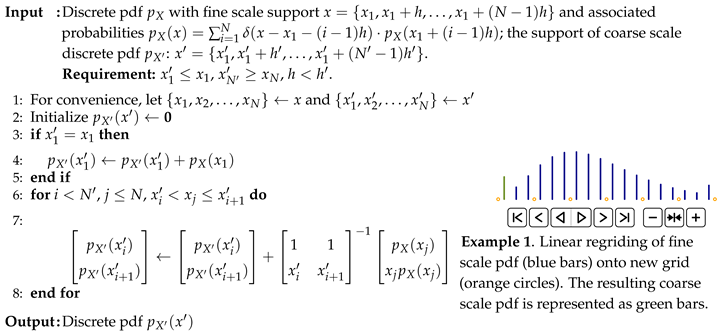
Algorithm 3: Linear regriding

In Stage I, a probability mass is dispersed to the two neighboring points and the two end points (first and last point on the new grid) such that the mean and the second moment are preserved. The local linear system for matching moments (Algorithm 4, Step 15) guarantees (i) positive masses added to the neighboring points and negative masses added to the end points, (ii) probabilities added to the neighboring points are inversely proportional to distances between these neighboring points and the projecting point. Property (ii) mimics linear regriding and completes a $4\times 4$ invertible local linear system along with the other three constraints for matching moments. Negative probabilities resulted from solving the system are typically small in absolute value because the end points are usually far from the projecting point. In practice, Stage I rarely leaves negative probabilities at one or both endpoints of the new grid on completion of the algorithm.

If this is not the case, in Stage II, the negative probability at the first (last) point is dispersed to the second (second to last), the third (third to last), and the last (first) point, respectively, subject to second order moment matching, see Steps 6 and 16 in Algorithm 5. The local linear system in step 7 (or 17) guarantees positive mass dispersed to the third (third to last) point and negative masses to the first (last) point and to the second (second to last) point respectively, see animation in Algorithm 5. Probability at the first (last) point is then set to zero and the second (second to last) point becomes the first (last) point on the new grid, reducing min/max range of $p_{X^{\prime }}$ support. The algorithm alternates between the first and the last points until both hold nonnegative probabilities, or, until no more points are available for balancing out the negative probabilities (see the animation in Example 3, Algorithm 5). The latter indicates 4-point regriding failure and invokes linear regriding.

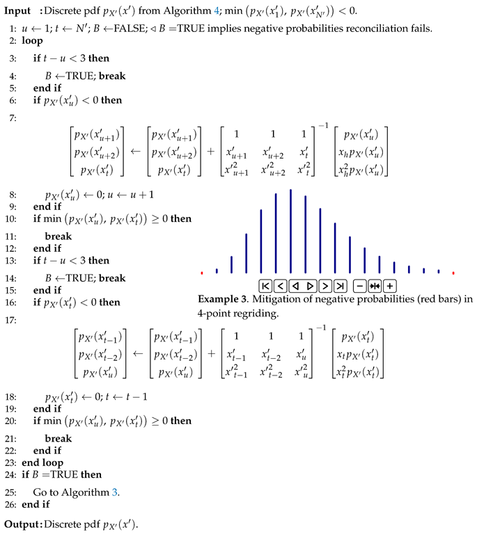
Algorithm 4: 4-point regridding, Stage I

Algorithm 5: 4-point regridding, Stage II

2.4.3. Comonotonization and Mixture Approximation

The basic construction idea for $p_S^{+}$ is listed in Algorithm 6 and illustrated by Example 3. The method proceeds recursively, defining the next element of the new distribution $p_S^{+}$ based on the first elements of $p_X$ and $p_Y$ then modifying $p_X$ and $p_Y$, respectively. It requires $O(N_x+N_y)$ operations.

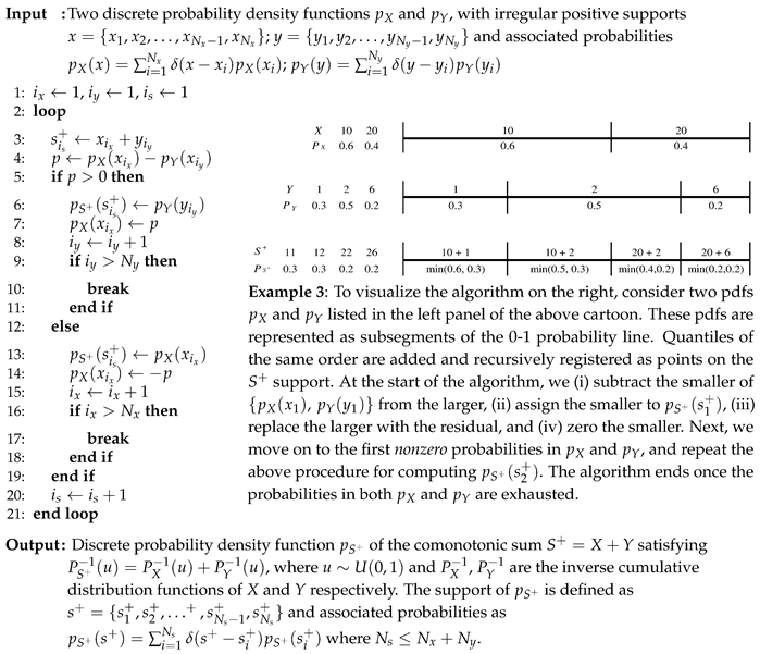
Algorithm 6: Distribution of the comonotonic sum

Once $p_{S^{\perp }}$, $p_{S^{+}}$ and w are known, the mixture distribution $p_S$ is composed using (11). In general, supports of $p_{S^{\perp }}$ and $p_{S^{+}}$ cover the same range but are defined on different individual grids, so arithmetizing on common grid is needed. If 4-point regriding is used, the target $\mathrm{E}[S]$ is preserved exactly and the target $\mathrm{Var}[S]$ is preserved with small error due to occasional retreats to linear regriding.

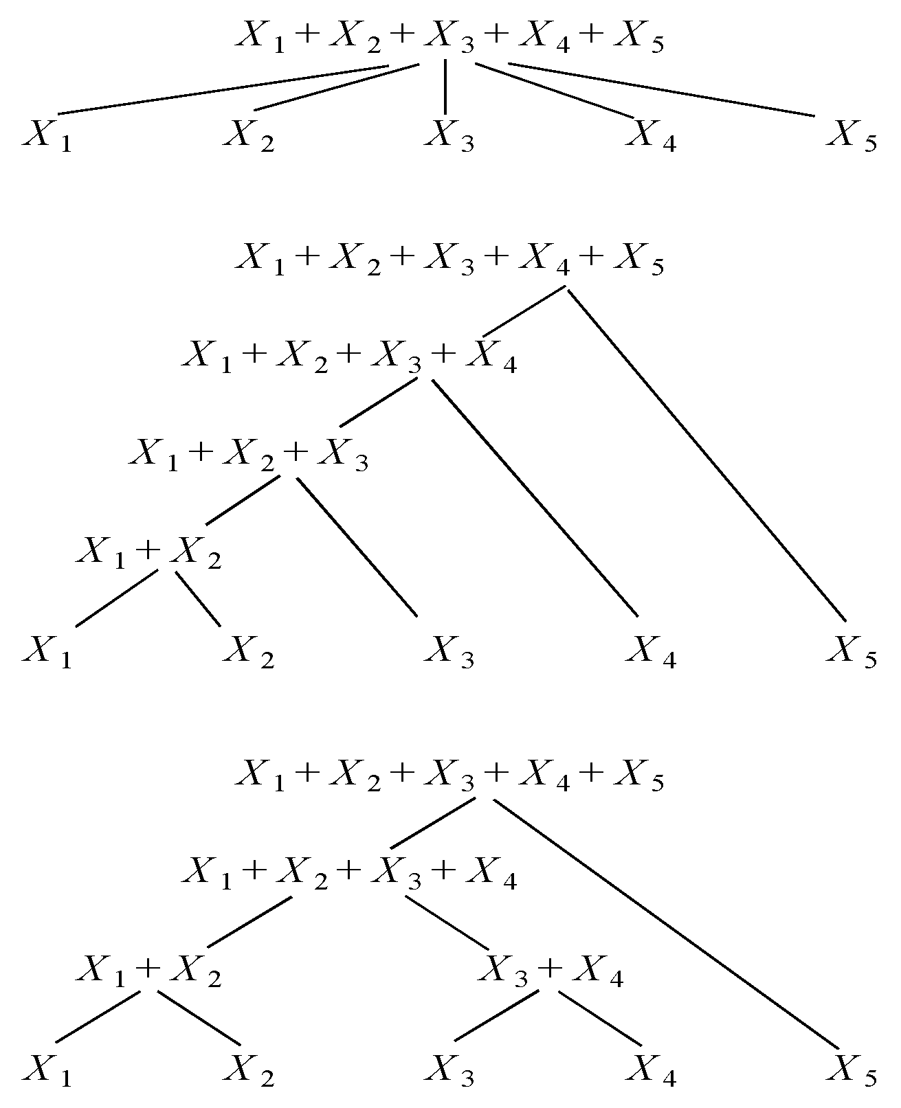
2.5. Order of Convolutions and Tree Topology

Following Wojcik et al. (2016), to further minimize this error, convolutions should be ordered to assure that two distributions undergoing convolution have supports covering approximately same domains ($x_{N_x}-x_1\approx y_{N_y}-y_1$) with the same span ($h_x\approx h_y$) in Algorithm 1. Since convolution is computationally more expensive than comonotonization, we assume that the order of convolutions governs the order of comonotonizations. Therefore, topology of a particular aggregation tree should be determined by the order of convolutions. For example, ascending order arranges risks at leaf nodes from smallest to largest maxima prior to aggregation, and then accumulates the risks using closest pair strategy depicted in the bottom panel of Figure 1. More sophisticated risk sorting strategy originates from the balanced multi–way number partitioning and is referred to as the balanced largest–first differencing method in Zhang et al. (2011). Here, one seeks to split a collection of numbers (risk maxima) into subsets with (roughly) the same cardinality and subset sum. In general, sorting based convolution orders are useful where no specific way to group risks at leaf nodes of aggregation tree is of importance for total risk analysis. When the goal is to assess the impact of spatial dependencies among elements within a CAT risk portfolio on aggregate loss, geographical grouping of properties (locations) affected by a particular CAT event is crucial (Einarsson et al. 2016). To account for such patterns we propose to use the recursive nearest neighbor order (RNN) of convolutions where depth-first search in Cormen et al. (2009) is performed to define an aggregation tree, see example in Figure 4. In contrast with sorting based strategies, the RNN keeps the original (predefined) ordering of risks at the leaf nodes of the aggregation tree intact.

It must be mentioned that order of convolutions is implicitly affecting the topology of the direct aggregation model in (7). This is shown in Figure 5 where the convex sum approximation at the root node is composed of aggregates constructed using, e.g., the RNN approach in Figure 4.

3. Results

As an example of loss analysis, we estimated ground-up loss for a major hurricane event in the US affecting 29,139 locations from portfolio of an undisclosed insurance company. Loss $X_k$ at kth location is described by inflated transformed beta pdf, i.e., the main part in (14) is parameterized using transformed beta in Venter (2013). We assume that the mean of each pdf is a function of CAT model prediction and that covariance between risks is a function of model error, so

$$\begin{array}{c}\hfill \begin{array}{cc}\hfill X_k& \sim InTrBeta({\Theta }_k)\hfill \\ \hfill \mathrm{E}(X_k)& =g(I_k)\hfill \\ \hfill \mathrm{Cov}(X_i,X_j)& ={\Sigma }_{i,j}=\mathrm{E}[(X_i-g(I_i))(X_j-g(I_j))]\hfill \end{array}\end{array}$$

(17)

where ${\Theta }_k$ is the parameter vector, $I_k$ stands for hurricane peril intensity end g is the damage function which transforms intensity into damage ratio. The intensity is expressed as wind speed and computed using the U.S. hurricane model in AIR-Worldwide (2015). Loss distributions are discretized on 64-point grid. Spatial dependency is described by $\mathbf{\Sigma }$ with nested block diagonal structure in Figure 2B. This structure is a consequence of using exchangeable correlation in spatial bins at two scales: 1 km and 20 km. The values assigned to off-diagonal elements of $\mathbf{\Sigma }$ are 0.07 if two locations belong to the same 1 km bin and 0.02 if two location belong to the same 20 km bin but different 1 km bins, respectively. Correlation between any two locations in different 20 km bins is set to zero. Details of our estimation methodology are given in Einarsson et al. (2016). Portfolio rollup was performed via direct, hierarchical sequential and hierarchical RNN models using Split-Atom convolution with linear and 4-point regriding. Note that for the hierarchical sequential model, the order of convolutions simply corresponds to the order of locations in insurance portfolio. The maximum number of points discretizing the aggregate distribution grid was set to 256. Additionally, to keep the discretization dense at the bulk of the aggregate distribution, we investigated the effect of right tail truncation at losses with probabilities $\le {10}^{-10}$.

The runs above were compared with Monte Carlo (MC) simulations. We applied Latin Hypercube Sampling in McKay et al. (1979) with sample reordering in Arbenz et al. (2012) to impose correlations between samples. We generated 30 realizations with 1 MM samples each. Second order statistics and Tail Value at Risk (or p%-TVaR, which measures the expectation of all the losses that are greater than the loss at a specified p% probability, see, e.g., Artzner et al. 1999; Latchman 2010) for these runs are presented in

Table 1. Mean ($\mu$), standard deviation ($\sigma$) and tail Value-at-Risk (TVaR_%) at levels 1%, 5% and 10% of the total hurricane risk for 29,139 locations for (A) direct, (B) hierarchical sequential and (C) hierarchical RNN aggregation models compared to the average values from 30 realizations of MC runs. The losses are in [$MM]. Numbers in brackets represent percentage errors relative to MC simulations.

		MC	Linear Regriding No Truncation	Linear Regriding Tail Truncation	4-Point Regridding
(A)	$\mu$		44.3	44.3 (0.00%)	44.3 (0.00%)	44.3 (0.00%)
	$\sigma$	7.1	10.9 (53.02%)	7.1 (0.00%)	7.1 (0.00%)
	TVaR1%	51.4	2550.9 (4864.2%)	2550.8 (4864.0%)	2550.8 (4863.9%)
	TVaR5%	48.5	502.1 (934.7%)	501.4 (932.8%)	501.9 (933.8%)
	TVaR10%	47.6	252.0 (429.7%)	250.7 (427.1%)	251.0 (427.6%)
(B)	$\mu$	44.3	44.3 (0.00%)	44.3 (0.00%)	44.3 (0.00%)
	$\sigma$	7.1	7.6 (6.11%)	7.1 (0.00%)	7.1 (0.00%)
	TVaR1%	93.7	81.2 (−13.3%)	84.7 (−9.6%)	88.0 (−6.1%)
	TVaR5%	66.3	62.5 (−5.8%)	68.5 (3.4%)	66.8 (0.8%)
	TVaR10%	58.6	67.3 (15.0%)	60.5 (3.3%)	59.8 (2.1%)
(C)	$\mu$	44.3	44.3 (0.00%)	44.3 (0.00%)	44.3 (0.00%)
	$\sigma$	7.1	7.2 (1.55%)	7.1 (0.00%)	7.1 (0.00%)
	TVaR1%	75.9	151.0 (98.9%)	95.0 (25.2%)	76.0 (0.1%)
	TVaR5%	62.9	184.4 (193.4%)	98.0 (55.8%)	63.5 (0.9%)
	TVaR10%	58.4	95.8 (63.9%)	87.0 (48.9%)	59.1 (1.1%)

. For the direct model, linear regriding inflates the variance of the total risk. This behavior is alleviated by tail truncation and/or 4-point regriding coupled with RNN order of convolutions. Variance of the total risk obtained from the sequential model with linear regriding and no truncation is higher than the corresponding variance of the RNN model. This is due to increasing size of the partial aggregate pdf support at upper branching nodes of the sequential tree as compared to that of the individual risks being cointegrated to these nodes. Again, tail truncation and 4-point regriding tackles this effect. For the RNN model, the reproduction of the tail statistics is poor if linear regriding is applied with or without tail truncation. These errors are reduced by 4-point method in Algorithms 4 and 5. Figure 6 shows comparisons between the aggregate distributions for direct and hierarchical models. Models based on linear regriding (the upper row) lead to coarse discretization of the final aggregation grid, with obvious shape mismatch between the sequential model and MC run. This is due to the lack of mechanism for keeping the dense discretization of the bulk of the total loss distribution and, for sequential model, due to increasing differences in max losses between partial aggregates and risks being cointegrated at branching nodes. Such mechanism is included in 4-point regriding (lower row in Figure 6). Interestingly, the grid of the total loss for direct model is still coarse.

Here, the support span of $p_{S^{+}}$ is much larger than that of $p_{S^{\perp }}$. Placing combination of both sums on the same grid causes the discretization of the comonotonic sum to dominate. Conversely, the bulk is well resolved by hierarchical models, however, only the RNN model reproduces the shape of the total loss distribution obtained from MC run.

Processing times of the investigated models are listed in

Table 2. Processing times [s] for different risk aggregation models. MC run is a single realization with 1 MM samples. The mixture method implementation for hierarchical trees was optimized for performance with nested block diagonal correlation structure in Figure 2B. Intel i7-4770 CPU @ 3.40 GHz architecture with 16 GB RAM was used.

Aggregation Model	MC	Linear Regridding No Truncation	Linear Regriding Tail Truncation	4-Point Regriding
Direct	1539	0.25	0.26	0.33
Hierarchical, sequential	12,769	0.34	0.35	0.44
Hierarchical, RNN	10,512	0.40	0.41	0.52

. Clearly, the proposed models outperform MC simulations. This is because (i) sampling from skewed loss distributions requires large sample size to resolve higher order moments of the total loss distribution while the implementation of the mixture method presented in the paper operates on 256-point grid and guarantees reproduction of the second order moments only, (ii) floating point addition (MC) and multiplication (the mixture method) have the same performance on (most) modern processors, (iii) large samples cause out-of-cache IO during reshuffling and sorting, i.e., the complexity O($NlogN)$ for fast sort does not apply.

Further, we investigated reproduction of the second order moments, 1,5,10%-TVaR and run times as a function of maximum grid size permitted during aggregation. These results are displayed in Figure 7. Oscillation of error curves (Figure 7A–E) is caused by variability in the total risk support size attributed to the maximum permitted grid size and to the risk aggregation scheme used. As expected, estimates of the mean ($\mu$) and the standard deviation ($\sigma$) perfectly reproduce their target values regardless of the support size. For small support sizes, the RNN model approximates TVaR better than sequential model (see Figure 7A–C). The pronounced underestimation of 1%-TVaR in Figure 7C is because 4-point regriding in Algorithm 5 eliminates negative probabilities at the expense of truncating min/max range of convolution and/or comonotonization support. The remedy is to increase the maximum support size. The sequential order has roughly linear growth of grid size because at the lth hierarchy of the sequential tree (see Figure 1), the left child node is always the aggregation of the first $l-1$ distributions, which guarantees the lth hierarchy has a grid size (before possible truncation) greater than that of the left child. The RNN order has nonlinear growth of grid size because for the lth aggregation, the two child nodes could be the aggregations of any number less than l of distributions, see Figure 4. In turn, grid sizes in the sequential run are larger on average than those in the RNN run. The latter yields higher speed shown in Figure 7F.

Oscillation of the computing time curves is mainly due to the cache mechanism (Hennessy and Patterson 2007, Chapter 5.5) in modern computer design. Varying support sizes leads to different cache miss frequencies during the entire run, and a cache miss is resolved by spending time reading from upper memory hierarchies. In consequence, a slightly larger support size could yield higher speed if it is better adapted to the cache hierarchies of the architecture where the program runs. A good example can be found at https://stackoverflow.com/questions/11413855/why-is-transposing-a-matrix-of-512x512-much-slower-than-transposing-a-matrix-of.

4. Conclusions

In this paper we presented several computationally fast models for CAT risk aggregation under spatial dependency. These models are variants of copula trees. Operations at branching nodes were facilitated by the Split-Atom convolution and estimation of distribution of the comonotonic sum. Using an example of ground-up loss estimation for 29,000 locations affected by a major hurricane event in the U.S., we have shown that the mixture method coupled with 4-point regriding and RNN order of convolutions, preserves target mean and variance of the total risk. Values of tail statistics compare favorably with those from, computationally slower, large sample MC runs.

5. Future Research Directions

In future work we aim to use the methods presented here for gross loss accumulation when complex financial terms act as non-linear transformations on partial loss aggregates in hierarchical trees. In such case the target second order statistics of the total risk are unknown and can only be inferred from MC runs. Since (sometimes nested) application of deductibles and limits makes the emergence of probability atoms even more pronounced than in the case of ground-up loss, fast gross loss aggregation strategies could potentially benefit from the Split-Atom approach. Another challenge is to develop a capital back allocation methodology which is in concert with our second order moment preservation requirement. This is crucial, for example, when risks in a geographical domain are part of one sub-limit by building and contents combined, and second sub-limit for business interruption; at the same time, some risks are not a part of any sub-limit.

Investigating how our methods can be extended to include negative correlations between pairs of risks is another exciting topic for future study. Some thoughts on this research direction are given in Appendix B.

References

1. AIR-Worldwide. 2015. AIR Hurricane Model for the United States. Available online: https://www.air-worldwide.com/publications/brochures/documents/air-hurricane-model-for-the-united-states-brochure (accessed on 5 May 2019).
2. Arbenz, Philipp, Christoph Hummel, and Georg Mainik. 2012. Copula based hierarchical risk aggregation through sample reordering. Insurance: Mathematics and Economics 51: 122–33. [Google Scholar] [CrossRef]
3. Artzner, Philippe, Freddy Delbaen, Jean-Marc Eber, and David Heath. 1999. Coherent measures of risk. Mathematical Finance 9: 203–28. [Google Scholar] [CrossRef]
4. Chaubey, Yogendra P., Jose Garrido, and Sonia Trudeau. 1998. On the computation of aggregate claims distributions: Some new approximations. Insurance: Mathematics and Economics 23: 215–30. [Google Scholar] [CrossRef]
5. Cherubini, Umberto, Elisa Luciano, and Walter Vecchiato. 2004. Copula Methods in Finance. Wiley Finance Series; Chichester: John Wiley and Sons Ltd. [Google Scholar]
6. Clark, K. 2015. Catastrophe Risk; International Actuarial Association/Association Actuarielle Internationale. Available online: http://www.actuaries.org/LIBRARY/Papers/RiskBookChapters/IAA_Risk_Book_Iceberg_Cover_and_ToC_5May2016.pdf (accessed on 5 May 2019).
7. Cormen, Thomas H., Charles E. Leiserson, Ronald L. Rivest, and Clifford Stein. 2009. Introduction to Algorithms, 3rd ed. Cambridge: MIT Press. [Google Scholar]
8. Côté, Marie-Pier, and Christian Genest. 2015. A copula-based risk aggregation model. The Canadian Journal of Statistics 43: 60–81. [Google Scholar] [CrossRef]
9. Denuit, Michel, Jan Dhaene, and Carmen Ribas. 2001. Does positive dependence between individual risks increase stop-loss premiums? Insurance: Mathematics and Economics 28: 305–8. [Google Scholar] [CrossRef]
10. Dhaene, Jan, Michel Denuit, Marc J. Goovaerts, Rob Kaas, and David Vyncke. 2002. The concept of comonotonicity in actuarial science and finance: Theory. Insurance: Mathematics and Economics 31: 3–33. [Google Scholar] [CrossRef]
11. Dhaene, Jan, Daniël Linders, Wim Schoutens, and David Vyncke. 2014. A multivariate dependence measure for aggregating risks. Journal of Computational and Applied Mathematics 263: 78–87. [Google Scholar] [CrossRef]
12. Einarsson, Baldvin, Rafał Wójcik, and Jayanta Guin. 2016. Using intraclass correlation coefficients to quantify spatial variability of catastrophe model errors. Paper Presented at the 22nd International Conference on Computational Statistics (COMPSTAT 2016), Oviedo, Spain, August 23–26; Available online: http://www.compstat2016.org/docs/COMPSTAT2016_proceedings.pdf (accessed on 5 May 2019).
13. Evans, Diane L., and Lawrence M. Leemis. 2004. Algorithms for computing the distributions of sums of discrete random variables. Mathematical and Computer Modelling 40: 1429–52. [Google Scholar] [CrossRef]
14. Galsserman, Paul. 2004. Monte Carlo Methods in Financial Engineering. New York: Springer. [Google Scholar]
15. Gerber, Hans U. 1982. On the numerical evaluation of the distribution of aggregate claims and its stop-loss premiums. Insurance: Mathematics and Economics 1: 13–18. [Google Scholar] [CrossRef]
16. Grossi, Patricia, Howard Kunreuther, and Don Windeler. 2005. An introduction to catastrophe models and insurance. In Catastrophe Modeling: A New Approach to Managing Risk. Edited by Patricia Grossi and Howard Kunreuther. Huebner International Series on Risk. Insurance and Economic Security. Boston: Springer Science+Business Media. [Google Scholar]
17. Hennessy, John L., and David A. Patterson. 2007. Computer Architecture: A Quantitative Approach, 4th ed. San Francisco: Morgan Kaufmann. [Google Scholar]
18. Hürlimann, Werner. 2001. Analytical evaluation of economic risk capital for portfolios of gamma risks. ASTIN Bulletin 31: 107–22. [Google Scholar] [CrossRef]
19. Iman, Ronald L., and William-Jay Conover. 1982. A distribution-free approach to inducing rank order correlation among input variables. Communications in Statistics-Simulation and Computation 11: 311–34. [Google Scholar] [CrossRef]
20. Koch, Inge, and Ann De Schepper. 2006. The Comonotonicity Coefficient: A New Measure of Positive Dependence in a Multivariate Setting. Available online: https://ideas.repec.org/p/ant/wpaper/2006030.html (accessed on 5 May 2019).
21. Koch, Inge, and Ann De Schepper. 2011. Measuring comonotonicity in m-dimensional vectors. ASTIN Bulletin 41: 191–213. [Google Scholar]
22. Latchman, Shane. 2010. Quantifying the Risk of Natural Catastrophes. Available online: http://understandinguncertainty.org/node/622 (accessed on 5 May 2019).
23. Lee, Woojoo, and Jae Youn Ahn. 2014. On the multidimensional extension of countermonotonicity and its applications. Insurance: Mathematics and Economics 56: 68–79. [Google Scholar] [CrossRef]
24. Lee, Woojoo, Ka Chun Cheung, and Jae Youn Ahn. 2017. Multivariate countermonotonicity and the minimal copulas. Journal of Computational and Applied Mathematics 317: 589–602. [Google Scholar] [CrossRef]
25. McKay, Michael D., Richard J. Beckman, and William J. Conover. 1979. A comparison of three methods for selecting values of input variables in the analysis of output from a computer code. Technometrics 21: 239–45. [Google Scholar]
26. McNeil, Alexander J., and Johanna Nešlehová. 2009. Multivariate Archimedean copulas, d-monotone functions and l1–norm symmetric distributions. The Annals of Statistics 37: 3059–97. [Google Scholar] [CrossRef]
27. Nelsen, Roger B. 2006. An Introduction to Copulas. Springer Series in Statistics; New York: Springer. [Google Scholar]
28. Panjer, Harry H., and B. W. Lutek. 1983. Practical aspects of stop-loss calculations. Insurance: Mathematics and Economics 2: 159–77. [Google Scholar] [CrossRef]
29. Robertson, John. 1992. The computation of aggregate loss distributions. Proceedings of the Casualty Actuarial Society 79: 57–133. [Google Scholar]
30. Shevchenko, Pavel V. 2010. Calculation of aggregate loss distributions. The Journal of Operational Risk 5: 3–40. [Google Scholar] [CrossRef]
31. Venter, Gary G. 2001. D.e. Papush and g.s. Patrik and f. Podgaits. CAS Forum. Available online: http://www.casact.org/pubs/forum/01wforum/01wf175.pdf (accessed on 5 May 2019).
32. Venter, Gary G. 2013. Effects of Parameters of Transformed Beta Distributions. CAS Forum. Available online: https://www.casact.org/pubs/forum/03wforum/03wf629c.pdf (accessed on 5 May 2019).
33. Vilar, José L. 2000. Arithmetization of distributions and linear goal programming. Insurance: Mathematics and Economics 27: 113–22. [Google Scholar] [CrossRef]
34. Walhin, J. F., and J. Paris. 1998. On the use of equispaced discrete distributions. ASTIN Bulletin 28: 241–55. [Google Scholar] [CrossRef]
35. Wang, Shaun. 1998. Aggregation of correlated risk portfolios: Models and algorithms. Proceedings of the Casualty Actuarial Society 85: 848–939. [Google Scholar]
36. Wojcik, Rafał, Charlie Wusuo Liu, and Jayanta Guin. 2016. Split-Atom convolution for probabilistic aggregation of catastrophe losses. In Proceedings of 51st Actuarial Research Conference (ARCH 2017.1). SOA Education and Research Section. Available online: https://www.soa.org/research/arch/2017/arch-2017-iss1-guin-liu-wojcik.pdf (accessed on 5 May 2019).
37. Zhang, Jilian, Kyriakos Mouratidis, and HweeHwa Pang. 2011. Heuristic algorithms for balanced multi-way number partitioning. Paper Presented at the International Joint Conference on Artificial Intelligence (IJCAI), Barcelona, Spain, July 16–22; Research Collection School Of Information Systems. Menlo Park: AAAI Press, pp. 693–98. [Google Scholar]
Figure 1. Aggregation of five risks using copula trees. Direct model (upper panel), hierarchical model with sequential topology (middle panel) and hierarchical model with closest pair topology (lower panel). The leaf nodes represent the risks whose aggregate we are interested in. The branching nodes of direct tree represent a multivariate copula model for the incoming individual risks while the branching nodes of hierarchical trees represent a bivariate copula model for the incoming pairs of individual and/or cumulative risks.
Risks 07 00054 g001
Figure 2. Illustration of hypothetical correlation matrices: (A) exchangeable, (B) nested block diagonal, and (C) unstructured correlation matrix.
Risks 07 00054 g002
Figure 3. A discrete loss pdf represented as a mixture of two “spikes” (atoms) at minimum and maximum x damage ratio (red) and the main part (blue). Damage ratio is discretized on 64-point grid.
Risks 07 00054 g003
Figure 4. An example of RNN approach for determining topology of hierarchical risk aggregation tree for six risks with zero minima. The maxima and cumulative maxima characterizing losses for the six risks are presented in the upper panel. (A) The algorithm takes the largest cumulative max and halves it to obtain the number c. Then, it binary searches for the number closest to c except for the last element in the sequence. This number (showed in bold) becomes the cumulative maximum of the new subsequence. The search is repeated until the subsequence consists of two elements. (B) The resulting hierarchical aggregation tree.
Risks 07 00054 g004
Figure 5. An example of recursive nearest neighbor (RNN) approach for determining topology of direct risk aggregation tree for six risks shown in Figure 4. Note that the order of comonotonic aggregation follows the order of independent aggregation.
Risks 07 00054 g005
Figure 6. MC (red line) and convolution/comonotoinization based (blue bars) distributions of the total risk for 29,139 locations affected by hurricane peril using different aggregation models with linear regriding (upper row) and 4-point regriding (lower row). No tail truncation was applied. For consistency, the losses are plotted in [0; $100 MM] interval.
Risks 07 00054 g006
Figure 7. (AE) Percentage errors in statistics of the total risk relative to the corresponding values obtained from MC simulations. Risk aggregation was performed for 29,139 locations affected by hurricane peril using sequential (blue) and RNN (red) models with 4-point regriding and maximum support size varying from 64 to 6400; (F) shows the average time cost of five runs for each maximum support size.
Risks 07 00054 g007