Abstract
We provide ready-to-use formulas for European options prices, risk sensitivities, and P&L calculations under Lévy-stable models with maximal negative asymmetry. Particular cases, efficiency testing, and some qualitative features of the model are also discussed.
1. Introduction
The pricing of financial derivatives, such as options, is an important yet difficult task in mathematical finance, in particular when one wishes to implement a model capturing realistic market patterns. Probably the most popular option-pricing model is the one introduced in Black and Scholes (1973); in this model, the instantaneous variations of an underlying asset are modeled by the geometric Brownian motion which, from the mathematical point of view, is described by the diffusion (or heat) equation. The Black-Scholes model has become popular among practitioners notably because of its simplicity, and because it admits a closed formula for the option price. However, the model fails in abnormal periods, typically during financial crises or periods of instability (Acharya and Richardson 2009); moreover, it does not reproduce observable features such as the shape of the volatility smile for short maturity, or the maturity pattern of the volatility smirk on equity index options markets (see Cont and Tankov 2004; Zhang and Xiang 2008). The main reason for this is that the Black-Scholes model is based on oversimplified assumptions, and, as a Gaussian model, underestimates the probability of large price jumps in real markets.
It is, therefore, necessary to introduce more appropriate models, with the capability to capture the complex behavior of financial markets. Many generalizations of the Black-Scholes model based on different approaches have been introduced. Let us mention, among the others, models based on stochastic volatility (Heston 1993), jump processes (Cont and Tankov 2004), regime switching models (Duan et al. 2002) or multifractals (Calvet and Fisher 2008). These generalizations are coming from very different fields, from econometric models to Econophysics and complex dynamical systems.
Particularly interesting are the generalizations based on fractional calculus. In this class of models, the underlying diffusion equation is extended to derivatives of non-natural order. These fractional derivative operators can be defined in many different ways, see e.g., Podlubny (1998) for a general overview. The main advantage of models based on such generalized diffusion equation lies in their ability to describe complex dynamics involving presence of large jumps, memory effects or risk redistribution (Kleinert and Korbel 2016). This class of fractional models include fractional Brownian motion pricing model (Necula 2008), mixed models (Sun 2013), models with time-fractional derivatives (Kleinert and Korbel 2016), or models with fractional diffusion of varying order (Korbel and Luchko 2016).
The first option-pricing model connected to generalized diffusion equation, introduced in Carr and Wu (2003) and called Finite Moment Log-Stable (FMLS) option-pricing model, makes the assumption that the instantaneous log returns of the underlying price are driven by a specific class of Lévy process; it is linked to fractional calculus because the model can equivalently be described by replacing the space derivative operator in the diffusion equation by the so-called Riesz-Feller fractional derivative. Historically, it was introduced by Carr and Wu to reproduce the maturity pattern of the implied volatility maturity smirk (the phenomenon that, for a given maturity, implied volatility are higher for out-of-the-money puts than for out-of-the-money calls); it is widely observed that the smirk (as a function of moneyness) does not flatten out as maturity increases, which is in contradiction with the Gaussian hypothesis: if the risk-neutral density were converging to the normal distribution, then the smirk would flatten for longer maturities. Carr and Wu deliberately violate the Gaussian hypothesis by assuming that the log returns of the market price are driven by a Lévy process and, when furthermore assuming that its distribution is strongly asymmetric (a fat left tail and a thin right tail), then the model generates the expected behavior for the implied volatility smirk. The tail index value (also known as stability parameter) of the Lévy process controls the negative slope of the smirk, which is flat when (Gaussian case) and becomes steeper when decreases, thus generating any observable slope in equity index options markets. Let us note that the maximal asymmetry assumption is plausible because large drops are more commonly observed in financial markets than large rises, and, moreover, ensures the option prices and all its moments to remain finite (which gave the name to the model).
The FMLS model is efficient when compared to other well-known models not only to generate complex volatility phenomena, but also to provide conservative valuations in the context of portfolio risk management (as demonstrated in Robinson 2015) and this makes it a good candidate for pricing and hedging. Unfortunately, the resulting option prices cannot be expressed in terms of elementary functions, which makes the model hard to use for practitioners. The main aim of this paper is therefore to provide a simple mathematical representation of the European option prices and related quantities (risk sensitivities, expected profit & loss) driven by the FMLS model, which can be easily used by any trader. Let us note that the use of fractional models would typically require the practitioner to implement advanced mathematical techniques such as integral transforms, complex analysis, or numerical methods; however, it has recently been shown that, for a wide class of space-time fractional option-pricing models, the option prices could be expressed in terms of rapidly convergent double series (Aguilar et al. 2018). The main advantage of this approach is that the resulting prices can be calculated without any advanced mathematical techniques or numerical methods, and with an arbitrary degree of precision; the proof is based on Mellin transform and residue summation in , and more details and applications can be found in Aguilar et al. (2018) and Aguilar and Korbel (2018). Since, as already mentioned, the FMLS model is a special case of generic space-time fractional models, this fruitful approach can be used for it as well to obtain efficient pricing tools. In this article, we will complete these results by developing additional analytic tools for hedging, for computing various market sensitivities and for P&L explanation, which constitute natural extensions to the double-series pricing formula.
The paper is organized as follows: Section 2 briefly summarizes the main aspects of the FMLS option-pricing model. It also presents the double sum representation of the option price. Section 3 introduces explicit formulas for the corresponding risk sensitivities (i.e., the Greeks) Delta, Gamma, and Theta. Section 4 discusses expected profit and loss under several hedging strategies. The ultimate section is devoted to conclusions.
2. Lévy-Stable Option Pricing
2.1. Model Definition
Let and let the market spot price of some underlying financial asset be described by a stochastic process on a filtered probability space . Following Carr and Wu (2003), we assume that there exists a risk-neutral measure under which the instantaneous variations of can be written in local form as:
where is the (continuous) risk-free interest rate, is the market volatility and is a standardized Lévy-stable process (see Cont and Tankov (2004) and references therein). The fact that the stochastic process is specified directly under the risk-neutral measure is clearly motivated by the option-pricing purpose; it is also justified by former models defined under the physical measure (see for instance McCulloch (1996) combining a Lévy-stable process under the physical measure, with a utility maximization argument to achieve finite option prices).
The solution to the stochastic differential Equation (1) is the exponential Lévy process:
where is the so-called “risk-neutral parameter”, which has its origin in the Esscher transform (see details in Gerber and Shiu (1994); Kleinert and Korbel (2016)) and, for an exponential process with density g, is defined by
where . Note that is the negative cumulant-generating function for . Since all cumulants are finite, the cumulant-generating function is also finite. The fact that the spot process admits the representation (2) shows that exponential Lévy models are a generalization of the Black-Scholes model: when then for any , degenerates into the usual Brownian motion and (2) becomes a geometric Brownian motion
thus recovering the Black-Scholes framework. The risk-neutral parameter in this case is the well-known term.
2.2. Stable Distributions
The probability distribution of the Lévy process is the -stable distribution that can be written under the form and is typically defined through the Fourier transform as (Zolotarev 1986):
where for and ; is called the stability parameter, and the asymmetry. In general, the two-sided Laplace transform of does not exist (which means that its moments diverge), except for the case (see e.g., Samorodnitsky and Taqqu 1994):
From a symmetry argument, it follows from (6) and definition (3) that the risk-neutral parameter is finite when and is equal to:
which justifies the choice in the model definition (1). Please note that we have introduced the -normalization so that we recover the Black-Scholes parameter when .
Under maximal negative asymmetry hypothesis , the asymptotic behavior of the distribution is determined by the stability parameter:
- −
- If , then decays exponentially on the positive real axis and has a heavy tail on the negative real axis (that is, decays in );
- −
2.3. Mellin-Barnes Representation of the European Option
Let ; the price of the European call option with strike K and maturity T is equal to the discounted -expectation of the terminal payoff
The expectancy in (8) is equal to the convolution of all possible realizations for the payoff with the probability distribution (or Green function) of the process:
The ratio is a temporal scaling exponent and allows to recover the Gaussian variance when (see more details in Kleinert and Korbel (2016)). After some algebraic manipulations, it is possible to re-write the Green function (5) as a Mellin-Barnes integral (see Flajolet et al. (1995) for a precise introduction to the Mellin transform), that is, an integral over a vertical line in the complex plane; precisely, it admits the representation:
The Green function connects the FMLS model to fractional calculus, because it is the fundamental solution to the space-fractional equation
where denotes the Riesz-Feller fractional derivative. When , it degenerates into the usual diffusion equation
which drives the Black-Scholes model. More details can be found in Mainardi et al. (2001).
Let us introduce the log-forward moneyness
so that we can re-write the payoff as . Plugging (10) into (9), integrating by parts and introducing the Mellin-Barnes representation for the exponential term (Bateman 1954)
yields, after integration on the parameter y, the following representation for the call price:
Proposition 1.
Let P be the polyhedra ; then, for any vector ,
2.4. Pricing Formulas
We now compute the double integral (15) by means of residue summation.
Theorem 1 (Pricing formula).
The European call option price is equal to the double sum:
Proof.
Let denote the differential form under the integral sign in (15); if we perform the change of variables
then reads
As the Gamma function is singular at every negative integer with residue (see Abramowitz and Stegun (1972) or any other monograph on special functions), it follows that in the region , has simple poles at every point , with residue:
The pricing Formula (16) is a simple and efficient way of pricing European call options under FMLS model; the convergence of partial sums is very fast and therefore only a few terms are needed to obtain an excellent level of precision, as demonstrated in Table 1 for a typical set of market parameters.

Table 1.
Numerical values for the -term in the series (16) for the option price (, ). The call price converges to a precision of after summing only very few terms of the series.
The price of the put option is easily deduced from (16) and the call-put parity relation ; with our notations (13), we get:
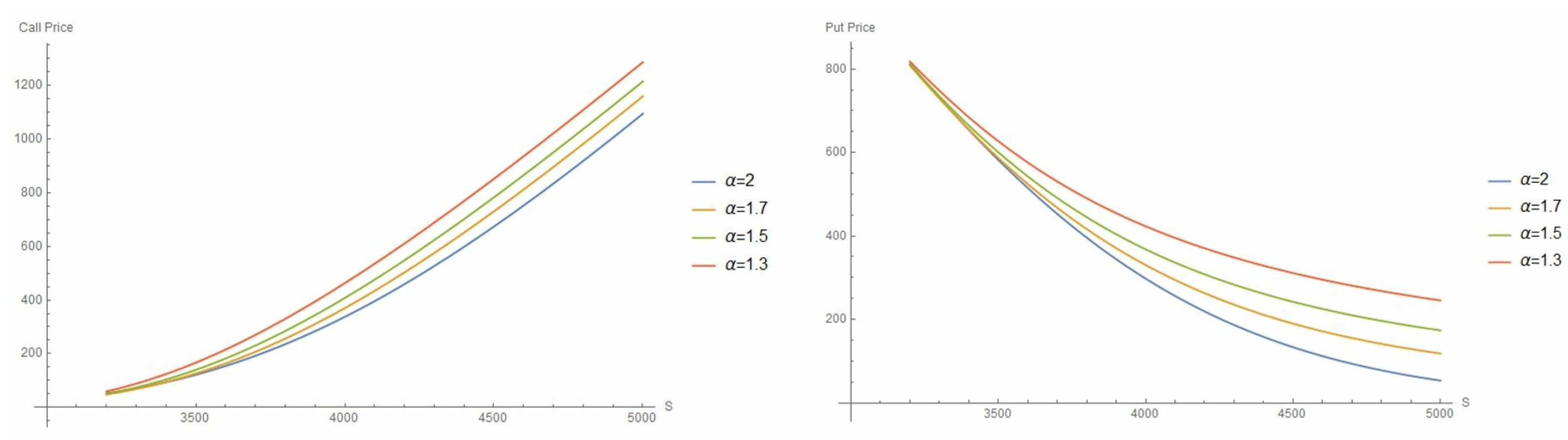
Typical shape of call and put prices is depicted in Figure 1.
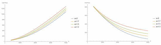
Figure 1.
Call (left graph) and put (right graph) option prices, as a function of S and for various stability parameters (parameters: , and ). In both the call and put cases, the prices become higher as decreases.
Particularly interesting situation occurs when the asset is at-the-money forward, that is, when or equivalently with our notations in Equation (16). In that case, it is immediate to see that:
Corollary 1 (At-the-money price).
When , the European call option price is equal to:
When (Black-Scholes model), then, by definition of , we are left with
As we have thus recovered the well-known Brenner-Subrahmanyam approximation (that was first introduced in Brenner and Subrahmanyam (1994)):
3. Risk Sensitivities (Greeks)
The Greeks quantify the sensitivity of the option to market parameters such as asset (spot) price or volatility, and are essential tools for portfolio management. In this section, we show that they admit efficient representations, which can be easily obtained by differentiation of the pricing Formula (16).
3.1. Delta
From the definition of k, we have and therefore, by differentiating (16) with respect to S and re-arranging the terms we obtain
This series is, again, very fast converging as demonstrated with typical values for the market parameters in Table 2. The Delta of the put option is easily obtained by differentiation of the call-put parity relation (20):
Table 2.
Numerical values for the -term in the series (25) for the call option’s Delta (, ).
When, moreover, (Black-Scholes model) then (27) becomes:
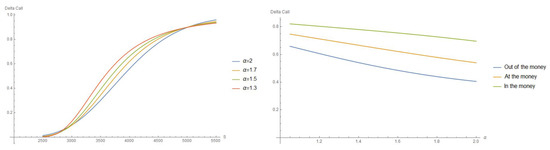
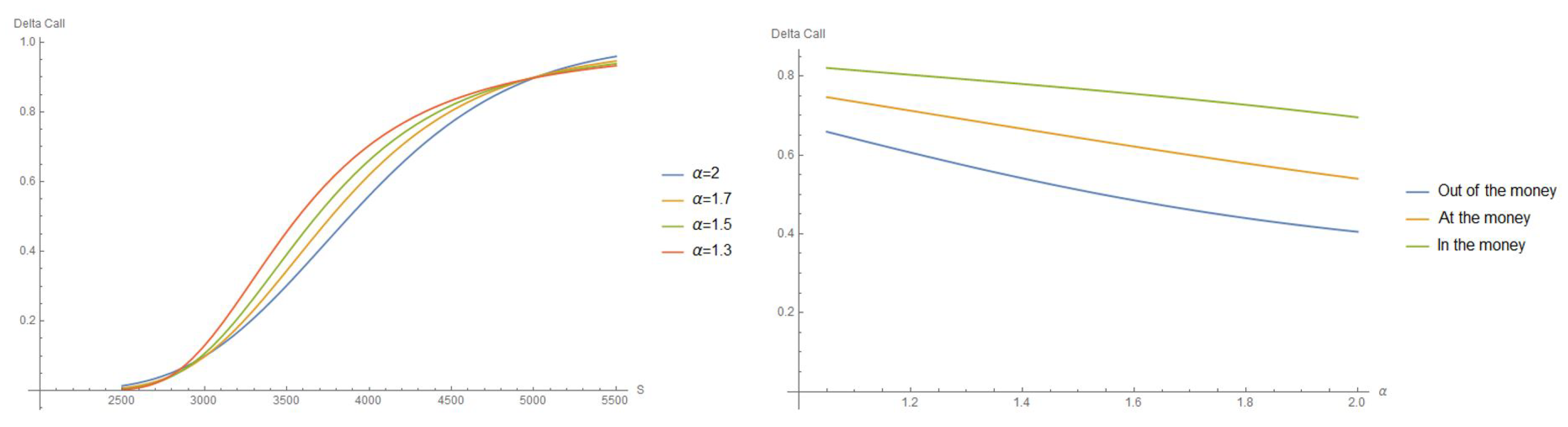
Figure 2.
(Left graph): Plot of the call’s Delta, in function of the market price S and for different stability parameters . (Right graph): Plot of the call’s Delta, in function of the stability parameter and for different market configurations. In both cases, , and .
- In left figure, we plot the value of in function of the market price, for different cases of ; in all cases, for all S, and admits an inflection in the “out-of-the-money” region (). However, we can observe that in this region, grows faster when decays, and the inflection occurs for smaller market prices.
- In the right figure, we choose 3 different values of S corresponding to the in, at or out-of-the-money situation and we plot the evolution of in function of . We can observe that is in all cases a decreasing function of (as could be expected from the overall factor in (25)) meaning that when becomes smaller, then the options become more sensitive to variations of the underlying price than in the Gaussian () case. This stronger sensitivity can be regarded as a conservative feature of the FMLS model (similar features have also been observed in Robinson (2015)).
3.2. Gamma
Differentiating the Call-Put relation for the Delta (26) with respect to S, it is immediate to see that the Gamma is the same for the call and the put options:
When, moreover, (Black-Scholes model) then (27) becomes:
3.3. Theta
By definition of k we have and therefore, by differentiating (16) with respect to and re-arranging the terms:
where
The Theta of the put option is easily obtained by differentiation of the call-put parity relation:
When the asset is at-the-money forward ( and therefore ), (35) reduces to:
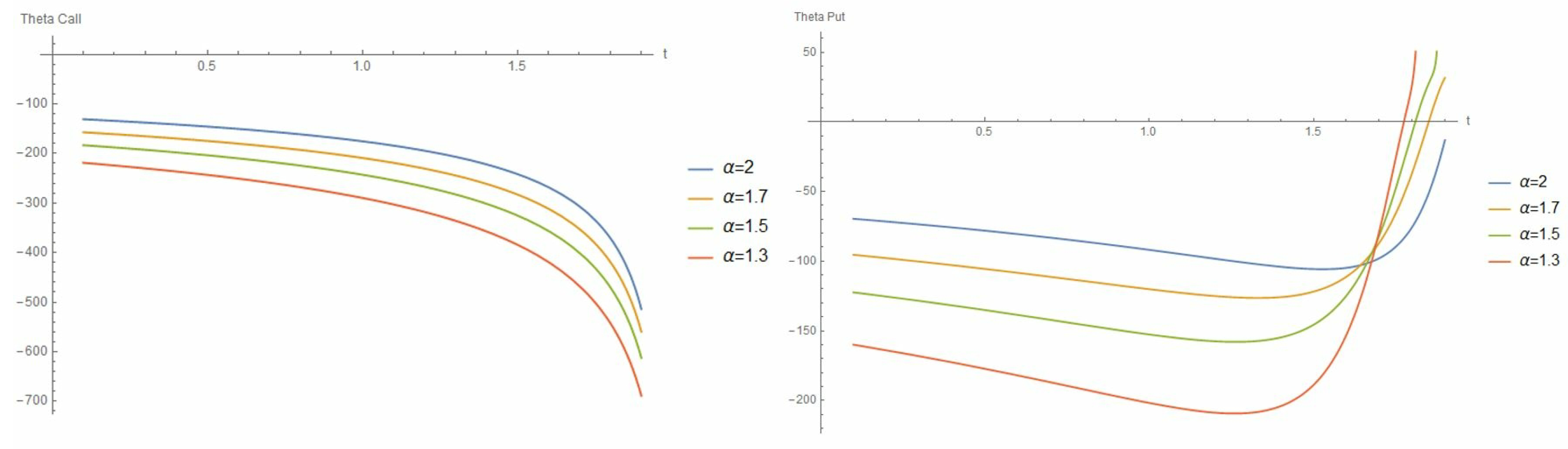
In Figure 3, we plot the evolution of . On the first graph, we fix and we observe that, as expected, is negative (as the value of the call can only decrease as time evolves), and becomes even more negative as decreases. Conversely, in graph 2 we show the time evolution of a deeply in the moment put option; in this configuration, when then the European call is identically null, that is and therefore and is positive. As illustrated by graph 2, this situation is accentuated when decreases.

Figure 3.
(Left graph): Theta of an at-the-money call (. (Right graph): Theta of a deeply in the money put (). In both cases , , and .
4. Expected P&L
Financial institutions are expected not only to compute the P&L of their trading desks, but also to produce an explanation of this P&L, both daily. The explanation should include passage of time as well as pure market effects such as price or volatility at first or second order (depending on the desired precision). In this section, we show how the sensitivity Formulas (25), (30) and (35) allow a fast and efficient explanation of P&L, for various examples of portfolios.
In the following, we consider call and put options on the S&P 500 index with maturity and strike price . The calculation will be made for each of the 22 trading days , of January 2019. Corresponding (normalized) time to maturity is defined to be
so that , etc. The underlying close prices at every are easily obtained via historical Bloomberg data for the ticker SPX Index.
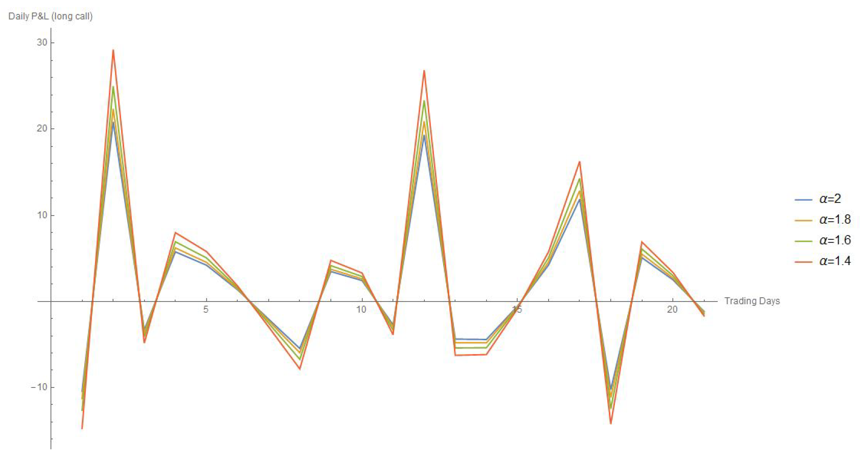
4.1. Long-Call Position
The daily P&L of a portfolio constituted of a call option only is equal to:
for . If we assume that the market volatility remains constant, it follows from Taylor’s formula that (40) can be approximated by:
where
for . We say that (40) is the real P&L, while (41) is the expected, or explained P&L. In Figure 4 we plot the evolution of the expected daily P&L for all the January trading period for different values of .

Figure 4.
Expected daily P&L of a long-call position, for various values of the stability parameter; one observes that daily losses or gains are accentuated when departs from 2.
The total P&L (real or expected) on the considered trading period is equal to:
and the total effects are obtained by summing the three components of the expected P&L (41):
In Table 3, we provide the monthly P&L explanation for the call option, as well as for the put; unsurprisingly, it is largely driven by the spot price effect which, in both cases, grows when decreases, resulting in a bigger gain (resp. smaller loss) in the call (resp. put) option case.
Table 3.
Monthly P&L explain for various portfolios on the S&P 500 and different stability parameters.
4.2. Delta-Hedged Portfolio
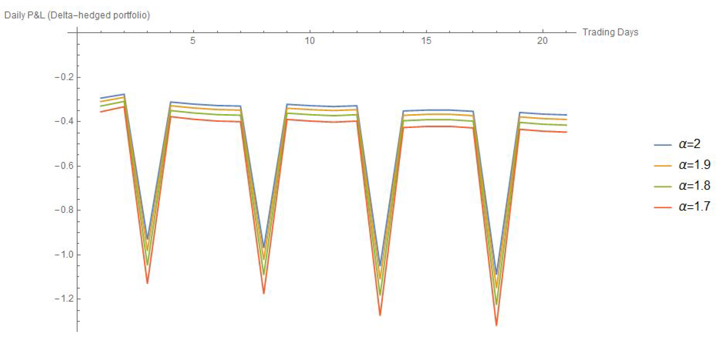
If the portfolio is appropriately delta-hedged at every trading day , for instance by holding a long-call position and a short position on the underlying then the Delta-dependence is eliminated and the expected daily P&L resumes to:
In Figure 5 we plot the expected daily P&L of the portfolio for various values of the stability. As market volatility is assumed constant, the portfolio is essentially driven by the passage of time with a typical daily P&L of −0.3, excepted when there are 3 days accrued (a situation occurring every 5 trading days and corresponding to weekends). Changes in do not alter this feature but slightly increase the daily loss of the portfolio. Total P&L and effects are presented in Table 3.
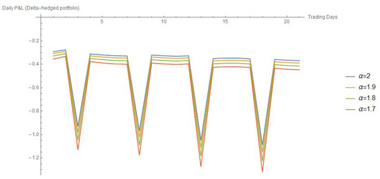
Figure 5.
Expected daily P&L of a delta-hedged portfolio; as before, the loss is accentuated when departing from the Gaussian case.
4.3. Gamma-Hedged Portfolio (Synthetic Future)
When the portfolio is long of a call and short of a put of same strike and maturity, then the Gamma and volatility risks are eliminated. The daily expected P&L is:
Please note that (46) is actually independent of because of the call-put parity relations (26) and (37):
and therefore the P&L will not be affected by the change of model. This is no surprise because holding a long-call and a short-put position is equivalent to holding a future contract, whose value is uniquely determined by the discounted value of the strike price.
5. Conclusions
In this paper, we have provided efficient formulas for computing the prices and risk sensitivities of European options under the FMLS model: they take the form of quickly converging double series, whose terms are straightforward to calculate without the need for any numerical scheme. We have also demonstrated that these formulas could be very conveniently used in the production and explanation of P&L, and provided several examples of portfolio calculations: as expected, the FMLS model is more “conservative” than the Black-Scholes model, in the sense that the options are more sensitive to stock prices variations and to the passage of time, resulting in notable variations in P&L when the Lévy parameter departs from 2.
We hope that the simple and efficient pricing and hedging tools provided in this paper will help popularizing stable option pricing (and non-Gaussian fractional models in general) to a broader community of capital market experts.
Author Contributions
J.-P.A. established and tested the results, both J.-P.A. and J.K. contributed to writing and revision of the manuscript.
Funding
J.K. was supported by the Austrian Science Fund (FWF) under project I3073 and by the Czech Science Foundation under grant 19-16066S.
Conflicts of Interest
The authors declare no conflict of interest.
References
- Abramowitz, Milton, and Irene A. Stegun. 1972. Handbook of Mathematical Functions. Mineola: Dover Publications, USA. [Google Scholar]
- Acharya, Viral V., and Matthew Richardson. 2009. Causes of the financial crisis. Critical Review 21: 195–210. [Google Scholar] [CrossRef]
- Aguilar, Jean-Philippe, Cyril G. Coste, and Jan Korbel. 2017. Non-Gaussian analytic option pricing: A closed formula for the Lévy-stable model. arXiv. [Google Scholar]
- Aguilar, Jean-Philippe, Cyril Coste, and Jan Korbel. 2018. Series representation of the pricing formula for the European option driven by space-time fractional diffusion. Fractional Calculus and Applied Analysis 21: 981–1004. [Google Scholar] [CrossRef]
- Aguilar, Jean-Philippe, and Jan Korbel. 2018. Option pricing models driven by the space-time fractional diffusion: Series representation and applications. Fractal and Fractional 2: 15. [Google Scholar] [CrossRef]
- Bateman, Harry. 1954. Tables of Integral Transforms (vol. I & II). New-York City: McGraw & Hill. [Google Scholar]
- Black, Fischer, and Myron Scholes. 1973. The Pricing of Options and Corporate Liabilities. Journal of Political Economy 81: 637–54. [Google Scholar] [CrossRef]
- Brenner, Menachem, and Marti G. Subrahmanyam. 1994. A simple approach to option valuation and hedging in the Black-Scholes Model. Financial Analysts Journal 50: 25–28. [Google Scholar] [CrossRef]
- Calvet, Laurent, and Adlai Fisher. 2008. Multifractal Volatility: Theory, Forecasting, and Pricing. Cambridge: Academic Press. [Google Scholar]
- Carr, Peter, and Liuren Wu. 2003. The Finite Moment Log Stable Process and Option Pricing. The Journal of Finance 58: 753–78. [Google Scholar] [CrossRef]
- Cont, Rama, and Peter Tankov. 2004. Financial Modelling With Jump Processes. New-York City: Chapman & Hall. [Google Scholar]
- Duan, Jin-Chuan, Ivilina Popova, and Peter Ritchken. 2002. Option pricing under regime switching. Quantitative Finance 2: 116–32. [Google Scholar] [CrossRef]
- Flajolet, Philippe, Xavier Gourdon, and Philippe Dumas. 1995. Mellin transform and asymptotics: Harmonic sums. Theoretical Computer Science 144: 3–58. [Google Scholar] [CrossRef]
- Gerber, Hans U., and Elias S. W. Shiu. 1994. Option Pricing by Esscher Transforms. Transactions of the Society of Actuaries 46: 99–191. [Google Scholar]
- Heston, Steven L. 1993. A Closed-Form Solution for Options with Stochastic Volatility with Applications to Bond and Currency Options. The Review of Financial Studies 6: 327–43. [Google Scholar] [CrossRef]
- Kleinert, H., and Jan Korbel. 2016. Option pricing beyond Black–Scholes based on double-fractional diffusion. Physica A 449: 200–14. [Google Scholar] [CrossRef]
- Korbel, Jan, and Yuri Luchko. 2016. Modeling of financial processes with a space-time fractional diffusion equation of varying order. Fractional Calculus and Applied Analysis 19: 1414–33. [Google Scholar] [CrossRef]
- Mainardi, Francesco, Yuri Luchko, and Gianni Pagnini. 2001. The fundamental solution of the space-time fractional diffusion equation. Fractional Calculus and Applied Analysis 4: 153–92. [Google Scholar]
- McCulloch, J. Huston. 1996. Financial applications of stable distributions. In Statistical Methods in Finance. Amsterdam: North-Holland, pp. 393–425. [Google Scholar]
- Necula, Ciprian. 2008. Option Pricing in a Fractional Brownian Motion Environment. Advances in Economic and Financial Research. DOFIN Working Paper Series 2; Bucharest, Romania: Bucharest University of Economics, Center for Advanced Research in Finance and Banking—CARFIB. [Google Scholar]
- Podlubny, Igor. 1998. Fractional Differential Equations: An Introduction to Fractional Derivatives, Fractional Differential Equations, to Methods of Their Solution and Some of Their Applications. Amsterdam: Elsevier, vol. 198. [Google Scholar]
- Robinson, Geoffrey K. 2015. Practical computing for finite moment log-stable distributions to model financial risk. Statistic and Computing 25: 1233–46. [Google Scholar] [CrossRef]
- Samorodnitsky, Gennady, and Murad S. Taqqu. 1994. Stable Non-Gaussian Random Processes: Stochastic Models with Infinite Variance. New-York City: Chapman & Hall. [Google Scholar]
- Sun, Lin. 2013. Pricing currency options in the mixed fractional Brownian motion. Physica A 392: 3441–58. [Google Scholar] [CrossRef]
- Zolotarev, Vladimir M. 1986. One-Dimensional Stable Distributions. Providence: American Mathematical Society. [Google Scholar]
- Zhang, Jin E., and Yi Xiang. 2008. The implied volatility smirk. Quantitative Finance 8: 263–84. [Google Scholar] [CrossRef]
© 2019 by the authors. Licensee MDPI, Basel, Switzerland. This article is an open access article distributed under the terms and conditions of the Creative Commons Attribution (CC BY) license (http://creativecommons.org/licenses/by/4.0/).