CEO Overconfidence and Shadow-Banking Life Insurer Performance Under Government Purchases of Distressed Assets

Abstract

In this paper, we develop a contingent claim model to evaluate the equity, default risk, and efficiency gain/loss from managerial overconfidence of a shadow-banking life insurer under the purchases of distressed assets by the government. Our paper focuses on managerial overconfidence where the chief executive officer (CEO) overestimates the returns on investment. The investment market faced by the life insurer is imperfectly competitive, and investment is core to the provision of profit-sharing life insurance policies. We show that CEO overconfidence raises the default risk in the life insurer’s equity returns, thereby adversely affecting the financial stability. Either shadow-banking involvement or government bailout attenuates the unfavorable effect. There is an efficiency gain from CEO overconfidence to investment. Government bailout helps to reduce the life insurer’s default risk, but simultaneously reduce the efficiency gain from CEO overconfidence. Our results contribute to the managerial overconfidence literature linking insurer shadow-banking involvement and government bailout in particular during a financial crisis.

1. Introduction

The bailout of American International Group (AIG) by the government taking 80% stake on 16 September 2008, was one of the defining moments of the financial crisis (Breitenfellner and Wagner 2010). The bailout was supported because the government perceived the near failure of AIG as too-big-to-fail and was not ready to have AIG fail.1 The 2008 global financial crisis raises fundamental issues about recapitalizing insurance institutions, particularly from the standpoint of insurer survival. In addition, a growing body of literature examines managerial overconfidence in financial decisions during a financial crisis (e.g., Fahlenbrach and Stulz 2011; Ma 2014; Ho et al. 2016). Our study also places stress on the chief executive officer (CEO) overconfidence. CEOs overestimate the returns on their investment projects and underestimate losses, incurring higher agency costs (Heaton 2002; Malmendier and Tate 2005). Berry-Stölzle et al. (2018) provide empirical evidence that CEO overconfidence associated with relatively low loss reserves results in increasing reported earnings. We extend this strand of the literature by examining the impact of the bailout on bankruptcy prediction when CEO overconfidence affecting investment decisions is considered in a life insurance company.2

We focus on a life insurance company for two reasons. First, life insurers are the business of providing policyholder protection from risks. Insurance helps economic activities by giving policyholder risk coverage and implicit confidence to make investments that they might otherwise deem too risky (Insurance Europe and Oliver Wyman 2013). Investment returns are an integral part of the life insurance policy itself. In particular, the level of guarantee that can be offered on the profit-sharing life insurance policies is directly affected by the available investments, while the level of participation on existing policies depends on the expected investment performance. A cognitive bias from CEO overconfidence becomes crucial to investment decisions of life insurers.3 Second, Harrington (2009) examines the role of AIG and its impact on the recent financial crisis. The author argues that the financial authority’s perception of AIG as “too big to fail” may have resulted in reducing the market discipline as it gives AIG an inappropriate competitive advantage. However, most previous studies on market structure in the life insurance literature have relied on an assumption of perfect competition.4 This assumption is not applicable to asset and life insurance policy markets since such markets are always highly concentrated where life insurers set rates and face random asset and policy levels, implicitly consistent with the “too big to fail” argument. Life insurance companies have unique features and provide a great natural laboratory for examining the effect of CEO overconfidence on insurer interest margin management in general. The insurer interest margin, defined as the spread between asset interest rate and guaranteed interest rate in our model, conveys vital information for the efficiency of insurer performance. As the spread is so important to insurer profitability, the issues of how it is optimally determined and how it adjusts to changes in the insurance environment deserve closer scrutiny.

In this paper, we examine the following questions that remain unanswered in the literature. First, what are the most likely effects of CEO overconfidence on the default risk in the shadow-banking life insurance company’s equity returns in particular when the optimal insurer interest margin is determined? The existing studies on this topic are largely silent on the optimal insurer interest margin determination. Second, how does the bailout program of buying distressed assets affect the efficiency gain/loss from CEO overconfidence? In this question, our primary emphasis is also the selection of the life insurance company’s optimal interest margin, which is generally not addressed in life insurance related work. In light of previous work, the purpose of this paper is to develop a contingent claim model to evaluate the equity and associated default risk of a life insurance company. The developed model of insurer spread behavior integrates the risk of a premature default to the equity return valuation along the line of Grosen and Jørgensen (2002) with managerial overconfidence, shadow insurance, and bailout considerations. The comparative static analyses of the model are investigated to determine the influence of CEO overconfidence on optimal insurer interest margin decisions and further on bankruptcy predictions.

Our contribution to the managerial overconfidence literature is threefold. First, we complement the literature on CEO overconfidence by improving on the perfectly competitive model and studying the dichotomous insurer interest margin determination. Our findings confirm the bankruptcy prediction that the life insurance company’s default risk is positively associated with CEO overconfidence at various levels of shadow-banking activity involvement or the bailout program of buying distressed assets. Second, we focus on the bailout program during a financial crisis by considering CEO overconfidence and confirming the bankruptcy prediction negatively associated with buying distressed assets at various levels of the cognitive bias from CEO overconfidence and shadow-banking activity involvement. Finally, we also complement the CEO overconfidence literature by elaborating on the issue of the efficiency gain/loss from insurer investment with CEO overconfidence in lieu of CEO rationality. The elaboration allows us to contribute to the topic of CEO overconfidence and financial crisis when the risk of a premature default to the valuation of a life insurance company is considered.

This paper is organized as follows. Section 2 reviews the related literature as a motivation of this study. Section 3 describes the model framework of a life insurance company. Section 4 theoretically discusses optimal decisions and comparative static analyses. Our numerical results are presented in Section 5. Section 6 concludes the paper.

2. Literature and Motivation

This section provides a literature review and presents the motivation of this study. First, in the psychology literature, the theory on managerial overconfidence is based on mis-calibration and the “better-than-average” effect (Alicke 1985; Moore and Healy 2008; Merkle and Weber 2011). Extrapolating from the psychology literature and the overinvestment view, Malmendier and Tate (2005), Goel and Thakor (2008), and Ben-David et al. (2013) argue that overconfident CEOs are convinced of their ability to generate higher returns on their investment projects, resulting in overinvestment. Hirshleifer and Luo (2001) predict that overconfident CEOs overvalue the prospects of borrowers (investors) and underestimate the riskiness of their investments. Adrian and Westerfield (2009) analyze a continuous-time principal-agent model with heterogeneous beliefs. Giat et al. (2009) complement the study of Adrian and Westerfield (2009) and develop a structural model to investigate the effects of asymmetric beliefs and agency conflicts on dynamic principal-agent relationships. By calibrating the model to data on pharmaceutical R&D projects, the authors show that optimism indeed significantly influences project values. Berry-Stölzle et al. (2018) study the relationships between CEO overconfidence and loss-reserving practices in the U.S. property-liability insurance industry. While we also elaborate the issue of managerial overconfidence and overinvestment, our focus on the CEO overconfidence aspects of a life insurer takes our analysis in a different direction.

The second strand is the literature on the channel from which CEOs influence investment. CEOs affect the quality of the information available to the board of directors and investors as well as corporate investment decisions (e.g., Adams and Ferreira 2007). Goel and Thakor (2008) find that the board is likely to end up with a pool of overconfident managers from which to choose a CEO and that moderate degrees of overconfidence actually benefit the shareholders. Dyreng et al. (2010) argue that a CEO can affect tax avoidance by setting the “tone at the top” with regard to the firm’s tax activities. This seems to suggest that even if (overconfident) CEOs do not directly influence investment decisions, they influence these decisions that are made by, for example, a CEO or other managers within the firm by having an aggressive personality or by hiring individuals with similar mindsets.5 A potential issue with using the “tone at the top” argument is that in this particular setting not only do CEOs not directly make the decision, but in many cases investment decisions for life insurers are made external to the firm by investment advisors (e.g., Kim et al. 2017).6 Our modeling provides a new perspective on how CEO overconfidence affects corporate investment decisions; the introduction of CEO overconfidence into the model makes the life insurers now face a trade-off between risky asset payments and net liabilities. Our results provide a useful complement to the argument on the channel from which CEOs influence corporate investment.

The third one is the recent literature on how the life insurance company gets involved in shadow-banking activities.7 Pozsar et al. (2013) point out that the life insurance company may also get involved in shadow banking activities that take place without direct and explicit access to public sources of liquidity or credit backstops. Life insurers adapted to regulatory policies, and over the years have made extensive use of captive reinsurance or shadow insurance as a way to circumvent stricter reserve requirements and artificially boost risk-based capital ratios; Irresberger and Peng (2017) discuss shadow insurance as a new form of regulatory arbitrage used by U.S. life insurers. Insurance Europe (2014) addresses the most common shadow-banking activities, including insurance securitization, catastrophe bonds, mortgage insurance, and securities lending, in which insurers engage, explaining why they are being undertaken as well as the potential benefits and associated risks. Irresberger and Peng (2017) study shadow insurance usage and capital management in life insurance groups. One of their main findings demonstrates that reinsurance agreements with shadow insurers are used by large and well capitalized insurance groups that deviate from their optimal structure. Our work is related to the literature on shadow-banking engagement on the asset side of the balance sheet where life insurers take some investment risk, in particular considering managerial overconfidence impacting insurer investment decisions.

The fourth is a growing body of literature on government bailout, focusing on the insurance industry. For example, Berry-Stölzle et al. (2014) argue that the government bailout through the Capital Purchase Program to assist U.S. life insurers during the 2008 financial crisis is unnecessary. According to their argument, there is no change in behavior in life insurers’ demand for capital during the financial crisis. Niehaus (2014) also concludes that there is no evidence of a differential relationship between life insurers’ internal capital flows and their fundamentals during the financial crisis. Barnes (2016) addresses the following crucial question. Did life insurers benefit from TARP or regulatory forbearance during the financial crisis of 2008–2009? An important answer addresses that regulatory forbearance acts as a substitute for the receipt of TARP funds. Lin et al. (2018) investigate how a bank’s default risk is affected by distress acquisition. The authors find that the acquirer bank incentivized by the government’s purchases of distressed loans under a certain level is likely to proceed with the distress acquisition. Under the circumstances, loan purchase assistance, as such, makes the bank less prone to risk-taking, thereby contributing to the stability of the banking system. Gómez and Ponce (2018) propose a formal model to study the optimal regulation of insurance firms. The authors find that in the absence of systemic risk, the optimal regulation may be implemented by capital regulation and by actuarially fair technical reserve. However, these instruments are not sufficient when insurance companies are exposed to systemic risk. Hsieh et al. (2014) show that before the Sarbanes Oxley Act of 2002 (SOX), companies of overconfident CEOs were more likely than other CEOs to engage in managing earnings through accelerating the timing of cash flow from operations and achieving analyst forecast benchmarks. From a regulatory perspective, their results illustrate that SOX was at least partially successful in curbing some overly aggressive earnings management behaviors. The primary difference between our model and these papers is that we consider the effects of managerial overconfidence on insurer interest margin and associated bankruptcy prediction, explicitly considering TARP and shadow insurance during a financial crisis.

3. Model Framework

This section consists of four parts. A few simplifying assumptions are made in the first part. The remaining three parts focus on the valuation of the life insurance company’s equity, the efficiency gain/loss from CEO overconfidence, and the bankruptcy prediction.

3.1. Assumptions

We develop a contingent claim model to evaluate the equity of a life insurance company. All economic decisions are made and values are determined with a one-period horizon with two dates, 0 and 1, $t\in [0,\hspace{0.17em}1]$. Since our goal is to demonstrate the distortionary behavior of overconfidence, we are silent on agency problems and assume that the insurer’s manager maximizes the shareholder value. The only friction in the model comes from the insurer manager’s inflated perception of the insurer investment opportunities. This perception follows Malmendier and Tate (2005).

By applying Grosen and Jørgensen (2002), the equity of the life insurance company can be viewed as a down-and-out call option on the company’s earning-asset portfolio where default can occur at any time before the maturity date. The risk of a premature default is introduced, which is most likely to describe the life insurance company in distress. This is the reason that the shareholders of the life insurance company are recognized as the residual claimants on the company’s assets after all other liabilities have been met. The strike price of the down-and-out call option is the book value of the company’s liabilities when the value of the company’s assets is less than the strike price, the company’s equity value equals zero. The scenario indicates that shareholders have a limited liability, and if the life insurance company is declared insolvent at $t=1$, they simply walk away. Under the scenario, life insurance policyholders (also liability holders) receive only what is left. When our model is developed, this story becomes clear.

As in the original work of Grosen and Jørgensen (2002), we assume that at time $t=0$, the life insurance company owns a capital structure as illustrated in the balance sheet of

Table 1. The life insurance company’s balance sheet at $t=0$.

Assets		Liabilities and Equity
Assets	A	Liabilities	$L=\alpha A$
		Equity	$K=(1-\alpha )A$
Total	A	Total	$A$

. That is, for simplicity, we suppose that the liability holder, also the representative policyholder, whose premium payment at $t=0$ constitutes the liability of the life insurance company, denoted by $L=\alpha A$ with $0<\alpha <1$, and the representative equity holder whose equity is accordingly denoted by $K=(1-\alpha )A$ form a mutual company, the life insurance company. $\alpha A$ denotes the proportion of the initial assets financed by liabilities, while $(1-\alpha )A$ denotes that financed by equity. Leverage α is a decision variable of the life insurance company.

.

In our model, the initial portfolio of assets is assumed to be totally invested in risky assets subject to non-performance. Assets granted by the life insurance company belong to a single homogeneous class of fixed-rate claims with $t\in [0,\hspace{0.17em}1]$. The demand of assets faced by the life insurance company is specified as a downward-sloping function $A(R_A)$ where $R_A$ is the asset interest rate. The assumption of $\partial A/\partial R_A<0$ implies that the life insurance company exercises some monopoly power in the asset market. Asset market as such is virtually always highly concentrated where the life insurance company sets rates and faces random asset levels. In addition, the investment rationally generates a stochastic future return $(1+R_A)A$ realized at $t=1$. The overconfident CEO overestimates future returns by percentage ${\alpha }_A\ge 0$.8 This overestimation is due to Choi et al. (2018) that CEO overconfidence noted in mis-calibration and the “better-than-average” effect reveals a tendency in CEOs’ overestimation of future payoffs on their investments.9 Hence, for all levels of investment, the CEO perceives the expected return to be $(1+R_A)(1+{\alpha }_A)A$, with ${\alpha }_A=0$ in the benchmark case of a rational CEO.10 The CEO overconfidence formulated in our model is consistent with the theoretical prediction that overconfident CEOs overestimate the returns on their investment projects (Berry-Stölzle et al. 2018). Results to be derived from our model do not extend to the case where CEO overconfidence may reveal underestimated liabilities on life insurance policies.

Besides CEO overconfidence, the life insurance company in distress is assumed to be willing to participate in the bailout program of buying distressed assets by the government. We focus on the bailout program for a number of reasons.11 Hoshi and Kashyap (2010) argue that buying distressed assets is an appropriate way to recapitalize financial institutions. However, the authors conclude that the bailout program lacks efficiency since assets cannot be purchased for more than their economic value. The efficiency issue in the bailout program of buying distressed assets will be re-examined based on our developing a contingent claim model to evaluate the equity of a life insurance company. Hoshi and Kashyap (2010) also argue that a distressed financial institution may refuse government bailout if the bailout generates an adverse signal that the institution is expected to have high future losses. Here, this is not the case that we focus on. According to Table 1, the expected repayments from the asset investment at $t=1$ can be specified as $\theta (1+R_B)(1+{\alpha }_A)A$ in our model, where $R_B$ is the security-market interest rate and $\theta A$ with $0<\theta <1$ at $t=0$ is the amount of buying distressed assets by the government. The condition of $R_A>R_B$ implies that the purchase of the assets comes at a discount to the book value of $\theta A$. The difference between $R_A$ and $R_B$ is the discount, which can be treated as the opportunity cost of bailout participation. The bailout $\theta$ is a decision variable of the regulatory authority.

Total assets are financed partly by profit-sharing life insurance policies including two common features: an interest rate guarantee and the contribution principle which entitles the policyholder to a participation in the life insurance company’s investment surpluses (Briys and de Varenne 1994). The total payoff to the policyholder of such a life insurance contract at maturity consists of three parts: a guaranteed payment which is the initial premium payment compounded by the interest rate guarantee, a short put option resulting from the fact that the equity holder has a limited liability, and a bonus paying to policyholder a fraction $\delta$ of the positive difference of the actual performance of its share in the life insurance company’s asset portfolio and the guaranteed amount at maturity (Chen and Suchanecki 2007). Furthermore, our model is assumed to determine the guaranteed interest rate policyholders should require to fully compensate them for the risks they face. The model is also driven by an imperfectly competitive market assumption about life insurance policies (Hong and Seog 2018). Specifically, the supply of life insurance policies faced by the life insurance company is governed by a positive-sloping supply function $L(R)=\alpha (1+{\alpha }_A)A{e}^R$, where $R$ is the guaranteed rate chosen by the life insurance company. The condition of $\partial L/\partial R>0$ indicates that the life insurance company conducts some monopoly power in the life insurance contract market.

In addition to balance-sheet insurance activities, we assume that the life insurance company is also involved in shadow-banking entrusted loans permitted by the Gramm-Leach-Bliley Act. This model follows Li and Lin (2016) to frame the entrusted loan transaction.12 There are entrusted loans made by a trustor (a production firm in general) in the non-financial economy that is run through the life insurance company (the trustee) for legal reasons, but with the company indemnified from the credit risk of the borrowing firm by the trustor.13 In the model, the fund $M$ at $t=0$ is lent through the life insurance company to the borrowing firm at an interest rate $R_M$ as instructed by the trustor. The company helps collect $(1+R_M)M$ at $t=1$ from the borrowing firm on the behalf of the trustor. The life insurance company charges a commission fee $mM$, where $m>0$, for the shadow-banking service as well as the risk burden for the transaction. Note that the life insurance company is not providing the capital for shadow-banking transactions.

3.2. Equity

With information about CEO overconfidence, shadow banking, and government bailout, we are ready to develop a contingent claim model along the line of Grosen and Jørgensen (2002). Toward that end, we assume that the market value of the life insurance company’s asset portfolio $V$ follows a geometric Brownian motion of the form:

$$\frac{dV}{V}=\mu dt+(\sigma +\frac{{\alpha }_A{\sigma }^2}{2})dW,$$

(1)

where

$$V=(1-\theta )(1+R_A)(1+{\alpha }_A)A+(1+R_M)M,$$

and where $V$ is specified as the non-bailout value of the company’s risky-asset repayments in its investments with overconfidence and the entrusted loan repayments in the shadow banking activities. A standard Wiener process is $W$. $V$ is the expected value with an instantaneous expected rate of return $\mu$ and an instantaneous deviation of return $(\sigma +{\alpha }_A{\sigma }^2/2)$. More specifically, we argue that there is the potential for overconfident investment in the asset market, perhaps because the life insurance company has gained some inside information as to the quality of its asset portfolio. We adopt a very simple quadratic formulation where the instantaneous deviation raised is given by $(\sigma +{\alpha }_A{\sigma }^2/2)$. Here ${\alpha }_A$ measures the degree of overconfidence in investment in the asset market: the stronger it is, the more risky is overconfident investment relative to the rational case.

The life insurance company seeks to maximize its expected net equity:

$$S=Max\hspace{0.17em}\{0,\hspace{0.17em}Min\hspace{0.17em}[V-X,\hspace{0.17em}(1-\delta \alpha )V-(1-\delta )X]\},$$

(2)

where

$$X=\alpha (1+{\alpha }_A)A{e}^R-\theta (1+R_B)(1+{\alpha }_A)A+(1+R_M)M-mM,$$

and where net liabilities $X$ consist of four parts: a guaranteed fixed payment which is the initial premium payment compounded by the interest rate guarantee, a return payment from the bailout asset to the company, a payment to the trustor in the shadow-banking transaction, and a commission fee income. Equation (2) can be rewritten as:

$$S=Max\hspace{0.17em}[0,\hspace{0.17em}V-X]-\delta \alpha Max\hspace{0.17em}[0,\hspace{0.17em}V-\frac{X}{\alpha }].$$

(3)

The equity position is a hybrid position and its value as of time $t\in [0,\hspace{0.17em}1]$ is specified as:

$$S=C(V,\hspace{0.17em}X)-\delta C(\alpha V,\hspace{0.17em}\hspace{0.17em}X),$$

(4)

where the equity $S$ consists of two down-and-out call options: a long down-and-out call on the asset portfolio $V$ with the strike equal to the promised payment $X$, and a short down-and-out call offsetting exactly the bonus of the liability holder. Both down-and-out call options are specified as follows. The value of $C(V,\hspace{0.17em}X)$ in Equation (4) is given by a down-and-out call:14

$$C(V,\hspace{0.17em}X)=[VN(b_1)-X{e}^{-(R_B-R)}N(b_2)]-[V{(\frac{H}{V})}^{2\eta }N(b_3)-X{e}^{-(R_B-R)}{(\frac{H}{V})}^{2\eta -2}N(b_4)],$$

(5)

where

$$H=\beta X,0<\beta <1,$$

$$\eta =\frac{R_B-R}{{(\sigma +{\alpha }_A{\sigma }^2/2)}^2}+\frac{1}{2},$$

$$b_1=\frac{1}{\sigma +{\alpha }_A{\sigma }^2/2}(\ln \frac{V}{X}+(R_B-R)+\frac{{(\sigma +{\alpha }_A{\sigma }^2/2)}^2}{2}),$$

$$b_2=b_1-\frac{1}{\sigma +{\alpha }_A{\sigma }^2/2},$$

$$b_3=\frac{1}{\sigma +{\alpha }_A{\sigma }^2/2}(\ln \frac{H^2}{VX}+(R_B-R)+\frac{{(\sigma +{\alpha }_A{\sigma }^2/2)}^2}{2}),$$

$$b_4=b_3-\frac{1}{\sigma +{\alpha }_A{\sigma }^2/2},$$

and where $H=\beta X$ is specified as $V$ that triggers bankruptcy (that is the barrier or knock-out value of the life insurance company), and $\beta$ is defined as the barrier-to-debt ratio in the premature default mode. $R_B-R$ is the compounded riskless rate of return due to the specification of $X$. $N(\cdot )$ is the cumulative density function of the standard normal distribution. In Equation (5), the first term $[\cdot ]$ on the right-hand side can be interpreted as the value viewed as a standard call option on $V$ at the strike price of $X$, while the second term $[\cdot ]$ can be interpreted as the down-and-in call option, lying dormant until a barrier is breached. Thus, Equation (5) illustrates a barrier option on the asset portfolio with strike equal to the promised payment at any time before the maturity date, called the residual barrier option. Analogously, the specification of $C(\alpha V,\hspace{0.17em}X)$ is given by:

$$C(\alpha V,\hspace{0.17em}X)=[\alpha VN(d_1)-X{e}^{-(R_B-R)}N(d_2)]-[\alpha V{(\frac{H}{\alpha V})}^{2\eta }N(d_3)-X{e}^{-(R_B-R)}{(\frac{H}{\alpha V})}^{2\eta -2}N(d_4)],$$

(6)

where

$$d_1=\frac{1}{\sigma +{\alpha }_A{\sigma }^2/2}(\ln \frac{\alpha V}{X}+(R_B-R)+\frac{{(\sigma +{\alpha }_A{\sigma }^2/2)}^2}{2}),$$

$$d_2=d_1-\frac{1}{\sigma +{\alpha }_A{\sigma }^2/2},$$

$$d_3=\frac{1}{\sigma +{\alpha }_A{\sigma }^2/2}(\ln \frac{H^2}{\alpha VX}+(R_B-R)+\frac{{(\sigma +{\alpha }_A{\sigma }^2/2)}^2}{2}),$$

$$d_4=d_3-\frac{1}{\sigma +{\alpha }_A{\sigma }^2/2}.$$

3.3. Efficiency Gain Prediction

The return and the variance of the life insurance company’s equity explicitly taking CEO overconfidence into account reveal the potentially substantial benefits and costs of relationship insurance. A question that arises is the extent to which CEO overconfidence adds efficiency gain/loss to the life insurance company when providing its insurance services. As far as insurer equity risk is concerned, the variance of the life insurance company’s return ${\sigma }_S$ will then be given by the Ronn and Verma (1986) formula:

$${\sigma }_S=\frac{1}{2}{(\sigma +\frac{{\alpha }_A{\sigma }^2}{2})}^2[\frac{V}{C(V,\hspace{0.17em}X)}\frac{\partial C(V,\hspace{0.17em}X)}{\partial V}+\delta \frac{\alpha V}{C(\alpha V,\hspace{0.17em}X)}\frac{\partial C(\alpha V,\hspace{0.17em}X)}{\partial \alpha V}],$$

(7)

With information about $S$ in Equation (4) and ${\sigma }_S$ in Equation (7), we can now compare the risk/return efficiency gain/loss from CEO overconfidence behavior. We apply Ergungor (2005) and specify the life insurance company’s efficiency gain/loss differential as:

$$\Delta E=E(WF)-E(OF),$$

(8)

where

$$E(WF)=\frac{S({\alpha }_A>0)}{{\sigma }_S({\alpha }_A>0)},$$

$$E(OF)=\frac{S({\alpha }_A=0)}{{\sigma }_S({\alpha }_A=0)},$$

and where $E(WF)$ is defined as the ratio of equity return to equity standard deviation when CEO overconfidence reveals where ${\alpha }_A>0$, and $E(OF)$ is also defined as the ratio when CEO rationality reveals where ${\alpha }_A=0$ in our model. $\Delta E$ in Equation (8) can be viewed as the equity return differential, per unit of standard deviation, that accrues from insurer investment with CEO overconfidence in lieu of CEO rationality. $\Delta E>0$ can be interpreted as efficiency gain from CEO overconfidence behavior, whereas $\Delta E<0$ can be interpreted as efficiency loss.

3.4. Bankruptcy Prediction

In the following subsection, we illustrate one particular application of Equation (4) to the problem of bankruptcy prediction. We now use the model of Brockman and Turtle (2003) and adapt it to value the default probability in the life insurance company’s equity returns. The valuation of Equation (4) implies a risk-neutral default probability over the interval from $t\in [0,\hspace{0.17em}1]$. This default probability consists of the following two parts. The first one is the default probability that the life insurance company’s asset portfolio will be less than the book value of the company’s liabilities based on $C(V,\hspace{0.17em}\hspace{0.17em}X)$. In the same way, the second one is the default probability based on the valuation $\delta C(\alpha V,\hspace{0.17em}X)$. We can write the default probability as:

$$P=P(V,\hspace{0.17em}X)+\delta P(\alpha V,\hspace{0.17em}X),$$

(9)

where

$$P(V,\hspace{0.17em}X)=N(h_1)+e^{h_2}(1-N(h_3)),$$

$$h_1=\frac{1}{\sigma +{\alpha }_A{\sigma }^2/2}(\ln \frac{\beta X}{V}-(R_B-R)+\frac{{(\sigma +{\alpha }_A{\sigma }^2/2)}^2}{2}),$$

$$h_2=\frac{2}{{(\sigma +{\alpha }_A{\sigma }^2/2)}^2}((R_B-R)-\frac{{(\sigma +{\alpha }_A{\sigma }^2/2)}^2}{2})\ln \frac{\beta X}{V},$$

$$h_3=-\frac{1}{\sigma +{\alpha }_A{\sigma }^2/2}(\ln \frac{\beta X}{V}+(R_B-R)-\frac{{(\sigma +{\alpha }_A{\sigma }^2/2)}^2}{2}),$$

$$P(\alpha V,\hspace{0.17em}X)=N(k_1)+e^{k_2}(1-N(k_3)),$$

$$k_1=\frac{1}{\sigma +{\alpha }_A{\sigma }^2/2}(\ln \frac{\beta X}{\alpha V}-(R_B-R)+\frac{{(\sigma +{\alpha }_A{\sigma }^2/2)}^2}{2}),$$

$$k_2=\frac{2}{{(\sigma +{\alpha }_A{\sigma }^2/2)}^2}((R_B-R)-\frac{{(\sigma +{\alpha }_A{\sigma }^2/2)}^2}{2})\ln \frac{\beta X}{\alpha V},$$

$$k_3=-\frac{1}{\sigma +{\alpha }_A{\sigma }^2/2}(\ln \frac{\beta X}{\alpha V}+(R_B-R)-\frac{{(\sigma +{\alpha }_A{\sigma }^2/2)}^2}{2}).$$

This equation estimates only a risk-neutral default probability and provides a meaningful ranking of the life insurance company according to its susceptibility to failure at various levels of alternative parameters in our model. Our measure of default risk is used to examine the relationship between default risk and insurer equity returns. This measure can be also used to demonstrate the state of financial stability discussed in the later sections.

4. Optimal Decisions and Comparative Static Analyses

This section mainly consists of two parts. The first part examines the solutions to the life insurance company’s optimization problem. The second part theoretically considers the effects on the optimal solutions from changes in managerial overconfidence and buying distressed assets of the model.

4.1. Dichotomized Optimal Decisions

In the model, the life insurance company is assumed to set $R_A$ or $R$ to maximize the market value of the life insurer’s equity. Partially differentiating the equity function with respect to $R_A$ or $R$, the first-order conditions for the equity maximization are given by:

$$\frac{\partial S}{\partial R_A}=\frac{\partial C(V,\hspace{0.17em}X)}{\partial R_A}-\delta \frac{\partial C(\alpha V,\hspace{0.17em}X)}{\partial R_A}=0,$$

(10)

$$\frac{\partial S}{\partial R}=\frac{\partial C(V,\hspace{0.17em}X)}{\partial R}-\delta \frac{\partial C(\alpha V,\hspace{0.17em}X)}{\partial R}=0.$$

(11)

Based on assumptions, it is reasonable to believe that the equity function of Equation (4) is strictly concave, at least in the short run, where there are sufficient conditions of ${\partial }^{2}S/\partial R_A^2<0$ and ${\partial }^{2}S/\partial R^2<0$ for optima in a non-simultaneous decision environment. This decision is understood because life insurers do not raise debt to purchase financial assets to cover liabilities towards policyholders (Thimann 2014). It should be noted that while our model is based on the assumption of dichotomy, our results to be derived from our model do not extend to the simultaneous case.

The dichotomized optimal solutions are explained as follows.15 The first-order condition in Equation (10) determines the optimal $R_A$ where $R$ remains constant. The optimal $R_A$ is determined by the life insurance company where the marginal long position of $R_A$ equals the marginal short position of $R_A$, the latter being weighted by $\delta$. Alternatively, the first-order condition in Equation (11) determines the optimal $R$ where $R_A$ is fixed. The same pattern as Equation (10) applies. As in the model, asset and liability sides are dichotomized. First, since $R$ is not a choice variable of the life insurance company, examining the impacts of parameters on the optimal insurer interest margin, i.e., the spread between $R_A$ and $R$, is tantamount to examining that on the optimal $R_A$. We call such spread behavior asset-side interest margin management. Second, since $R_A$ is not a choice variable, examining the effects of parameters on the optimal insurer interest margin is tantamount to examining that on the optimal $R$. Similarly, we call such spread behavior liability-side interest margin management. It is recognized that insurer interest margin conveys vital information for the efficiency of the insurance system. Identifying the determinants of insurer interest margin would help to understand changing trends in insurance efficiency and provide implications for the regulatory insurance environment. These results are used in a later subsection when the comparative static effects are analyzed.

4.2. Overconfidence Effects

Here, the importance of CEO overconfidence is emphasized. Our following results address the issue: what are the most likely effects of the CEO overconfidence on the life insurance company’s interest margin and default risk? First, to capture the response of the optimal insurer interest margin to a change in CEO overconfidence, one implicitly differentiates Equation (10) with respect to ${\alpha }_A$ where $R$ remains constant, or Equation (11) with respect to ${\alpha }_A$ where $R_A$ remains constant, which yields the following:

$${\frac{\partial R_A}{\partial {\alpha }_A}|}_{R=\mathrm{constant}}=-\frac{{\partial }^{2}S}{\partial R_A\partial {\alpha }_A}/\frac{{\partial }^{2}S}{\partial R_A^2},$$

(12)

$${\frac{\partial R}{\partial {\alpha }_A}|}_{R_A=\mathrm{constant}}=-\frac{{\partial }^{2}S}{\partial R\partial {\alpha }_A}/\frac{{\partial }^{2}S}{\partial R^2}.$$

(13)

Equation (12) depicts the impact on the life insurance company’s asset interest rate (and thus the company’s asset-side interest margin) from changes in the level of CEO overconfidence. Equation (13) analyzes the impact on the life insurance company’s guaranteed interest rate (and thus the company’s liability-side interest margin) from changes in the level of CEO overconfidence. Theoretical explanations about both the scenarios will be represented in the next numerical section.

Second, we consider the impact of CEO overconfidence on the default risk in the life insurance company’s equity returns. Differentiation of Equation (9) evaluated at the optimal $R_A$ or the optimal $R$ with respect to ${\alpha }_A$ yields:

$${\frac{dP}{d{\alpha }_A}|}_{R=\mathrm{constant}}=\frac{\partial P}{\partial {\alpha }_A}+\frac{\partial P}{\partial R_A}\frac{\partial R_A}{\partial {\alpha }_A},$$

(14)

$${\frac{dP}{d{\alpha }_A}|}_{R_A=\mathrm{constant}}=\frac{\partial P}{\partial {\alpha }_A}+\frac{\partial P}{\partial R}\frac{\partial R}{\partial {\alpha }_A},$$

(15)

where the first term on the right-hand side of Equation (14) can be interpreted as the direct effect, while the second term can be interpreted as the indirect effect. The direct effect demonstrates the change in $P$ due to an increase in ${\alpha }_A$, holding the optimal $R_A$ constant. The indirect effect arises because of changed $P$ due to an increase in ${\alpha }_A$ through every possible optimal state of $R_A$. Equation (15) depicts the relationship between $P$ and ${\alpha }_A$, explicitly considering the adjustment of every possible optimal state of $R$. The same pattern as previously applies. The added complexity of path dependent options, in general, leads to complicated comparative static results of Equations (12)–(15). In the next section, we will calculate these comparative static results numerically to provide intuition.

4.3. Bailout Effects

Buying distressed assets by the government was one of the most important bailout programs during the 2007/2008 global financial crisis. In this subsection, we theoretically show how the bailout program can influence the life insurance company’s decision makings. First, to analyze the response of the optimal insurer interest margin to a change in the bailout program of buying distressed assets, one implicitly differentiates Equation (10) with respect to $\theta$ where $R$ remains constant, or Equation (11) with respect to $\theta$ where $R_A$ remains constant, which gives the following:

$${\frac{\partial R_A}{\partial \theta }|}_{R=\mathrm{constant}}=-\frac{{\partial }^{2}S}{\partial R_A\partial \theta }/\frac{{\partial }^{2}S}{\partial R_A^2},$$

(16)

$${\frac{\partial R}{\partial \theta }|}_{R_A=\mathrm{constant}}=-\frac{{\partial }^{2}S}{\partial R\partial \theta }/\frac{{\partial }^{2}S}{\partial R^2}.$$

(17)

Second, we examine the impact of buying distressed assets by the government on the life insurance company’s default risk. Since the derivation is analogous to that for the CEO overconfidence, we jump to the results:

$${\frac{dP}{d\theta }|}_{R=\mathrm{constant}}=\frac{\partial P}{\partial \theta }+\frac{\partial P}{\partial R_A}\frac{\partial R_A}{\partial \theta },$$

(18)

$${\frac{dP}{d\theta }|}_{R_A=\mathrm{constant}}=\frac{\partial P}{\partial \theta }+\frac{\partial P}{\partial R}\frac{\partial R}{\partial \theta }.$$

(19)

Third, since changes in the bailout program of buying distressed assets from the insurance company by the government can affect CEO overconfidence behavior, and thus efficiency gain/loss from CEO overconfidence, one differentiates Equation (8) with respect to $\theta$ when the optimal $R$ or $R_A$ is constant, giving:

$${\frac{d\Delta E}{d\theta }|}_{R=\mathrm{constant}}=\frac{\partial \Delta E}{\partial \theta }+\frac{\partial \Delta E}{\partial R_A}\frac{\partial R_A}{\partial \theta },$$

(20)

$${\frac{d\Delta E}{d\theta }|}_{R_A=\mathrm{constant}}=\frac{\partial \Delta E}{\partial \theta }+\frac{\partial \Delta E}{\partial R}\frac{\partial R}{\partial \theta }.$$

(21)

The first term on the right-hand side in Equation (20) can be explained as the direct effect, while the second term can be explained as the indirect effect. The direct effect demonstrates the change in the efficiency gain/loss from CEO overconfidence due to an increase in the buying distressed assets by the government, holding the optimal loan asset interest rate constant. The indirect effect describes the change in the efficiency gain/loss by $A(R_A)$ in every possible optimal state. The same interpretation as previously stated, applies to Equation (21). Again, given the chosen parameter values we will calculate the comparative static results based on Equations (16)–(21) to provide intuition regarding the bailout problems in the next section.

5. Numerical Analysis

According to the overconfidence and bailout effects introduced in the previous section, we can determine the comparative static results through a numerical combination of the parameters. In this section, we first assume some reasonable parameter values for the comparative static analyses. Next, as before, we consider two effects: CEO overconfidence and bailout.

5.1. Numerical Assumptions

The assumed numerical values based on our derived model are demonstrated as follows.

(i)

We follow Briys and de Varenne (1994) and assume $65\%\le \delta \le 95\%$, and $\sigma =0.30$ for the numerical analysis in the model.

(ii)

Let $(R_A(\%),\hspace{0.17em}A)$ faced by the life insurance company change from (5.50, 300.5) to (6.10, 269) due to the downward-sloping assumption.

(iii)

Let $(R\hspace{0.17em}(\%),\hspace{0.17em}L)$ change from (2.25, 285) to (3.75, 347) to capture the upward-sloping condition.

(iv)

Let the shadow-banking entrusted loans $M$ fluctuate from 60 to 80 with the commission rate of $m=0.10\%$.

(v)

We assume that $R_M=5.00\%$, and $R_B=4.00\%$. The condition of $R_A>R_M$ implies that the asset interest rate determined by the life insurance company is greater than the market rate of return from $M$ invested in the financial market. The condition of $R_M>R_B$ reasonably demonstrates a financial environment where the expected rate of return from the risky investment $M$ is greater than the security-market interest rate from buying distressed assets by the government.

(vi)

The initial barrier level is assumed to be set $\beta =0.60$ which are observed from an empirical barrier average estimated by Brockman and Turtle (2003).

(vii)

We assume that the degree range of overconfidence is $0.20\le {\alpha }_A\le 0.45$.

(viii)

Let the level of buying distressed assets $\theta$ increase from 0.40 to 0.65.

5.2. CEO Overconfidence Analysis

Due to the dichotomized optimization in our analysis, we consider the following two sets of the effects of CEO overconfidence behavior on either asset-side or liability-side interest margin management, and then on its default risk in the life insurance company’s equity returns.

The result based on Equation (12) is summarized in the second panel of

Table 2. Responsiveness of asset-side interest margin (asset interest rate) and default risk to CEO overconfidence degree based on Equations (12) and (14) ¹.

	$(R_A(\%),\hspace{0.17em}A)$
${\alpha }_A$	(5.50, 300.5)	(5.60, 300)	(5.70, 299)	(5.80, 297)	(5.90, 293)	(6.00, 285)	(6.10, 269)
	$S$
0.20	88.6904	88.7137	88.6163	88.2773	87.4542	85.6613	81.9249
0.25	91.5091	91.5327	91.4309	91.0780	90.2220	88.3579	84.4738
0.30	94.3162	94.3401	94.2339	93.8671	92.9782	91.0433	87.0121
0.35	97.1116	97.1359	97.0253	96.6446	95.7229	93.7173	89.5396
0.40	99.8956	99.9201	99.8050	99.4105	98.4562	96.3802	92.0566
0.45	102.6680	102.6927	102.5732	102.1649	101.1780	99.0319	94.5629
	$\partial R_A/\partial {\alpha }_A$(%)
0.20→0.25	-	0.6034	−3.6332	−5.7463	−6.7994	−7.3230	-
0.25→0.30	-	0.5230	−3.5086	−5.5196	−6.5217	−7.0200	-
0.30→0.35	-	0.4489	−3.3935	−5.3101	−6.2652	−6.7402	-
0.35→0.40	-	0.3805	−3.2868	−5.1161	−6.0277	−6.4811	-
0.40→0.45	-	0.3172	−3.1876	−4.9358	−5.8070	−6.2403	-
	$P$
0.20	0.1116	0.1111	0.1106	0.1101	0.1098	0.1097	0.1103
0.25	0.1146	0.1141	0.1135	0.1131	0.1127	0.1126	0.1132
0.30	0.1177	0.1171	0.1165	0.1161	0.1157	0.1156	0.1161
0.35	0.1208	0.1202	0.1196	0.1191	0.1188	0.1187	0.1191
0.40	0.1240	0.1234	0.1228	0.1223	0.1219	0.1218	0.1222
0.45	0.1272	0.1266	0.1260	0.1255	0.1251	0.1249	0.1254
	$dP/d{\alpha }_A:$ total effect (%),$R=$ constant
0.20→0.25	-	5.9360	5.9304	5.9088	5.8740	5.8210	-
0.25→0.30	-	6.0737	6.0678	6.0464	6.0123	5.9607	-
0.30→0.35	-	6.2055	6.1993	6.1781	6.1446	6.0944	-
0.35→0.40	-	6.3318	6.3253	6.3043	6.2714	6.2225	-
0.40→0.45	-	6.4531	6.4464	6.4256	6.3932	6.3455	-

¹ Parameter values, unless stated otherwise, $\delta =0.65$, $\sigma =0.30$, $m=0.10\%$, $\alpha =0.95$, $R_M=5.00\%$, $R_B=4.00\%$, $\beta =0.60$, $M=60$, $\theta =0.40$, and $R=2.25\%$. The second-order condition of Equation (10) is consistently confirmed by ${\partial }^{2}S/\partial R_A^2<0$. The shaded areas represent the values of $S$, $\partial R_A/\partial {\alpha }_A$, $P$, and $dP/d{\alpha }_A$ with the optimal $R_A=5.60\%$. The negative indirect effect, $(\partial P/\partial R_A)(\partial R_A/\partial {\alpha }_A)<0$, is insufficient to offset the positive direct effect, $\partial P/\partial {\alpha }_A>0$.

that CEO overconfidence is associated with the low amount of assets at an increased asset interest rate chosen by the life insurance company, resulting in low revenue earnings. Intuitively, as the overconfident CEO of the life insurance company overestimates future investment return (Malmendier and Tate 2005), the life insurance company must now provide a return to a higher behavioral bias base. One way the life insurance company may attempt to augment its total returns is by decreasing its asset investment at an increased asset interest rate. Malmendier and Tate (2005) provide empirical evidence that managerial overconfidence impacts corporate investment decisions. Further, our finding contributes the managerial overconfidence literature: if asset demand faced by the life insurance company is relatively rate-elastic, a lower asset earning is possible at an increased interest margin due to CEO overconfidence. In addition, the computed results based on Equation (14) are demonstrated in the last panel of Table 2 that CEO overconfidence is associated with high default risks. The positive direct effect captures the increase in $P$ due to an increase in ${\alpha }_A$, holding the optimal $R_A$ constant. This is because distortion in insurer investment may be a result of CEO overestimating the returns to his/her investment, resulting in increasing the default risk in the life insurance company’s equity returns. The negative indirect effect arises because (i) an increase in the CEO overconfidence increases the asset interest rate chosen by the life insurance company, and then (ii) a low amount of asset (and thus a less risky asset) is possible at an increased asset interest rate, yielding a lower level of default risk. Therefore, the negative indirect effect insufficiently offsets the positive direct effect to give a positive response of default risk to an increase in CEO overconfidence. Our result is in large consistent with the empirical findings of Berry-Stölzle et al. (2018).16

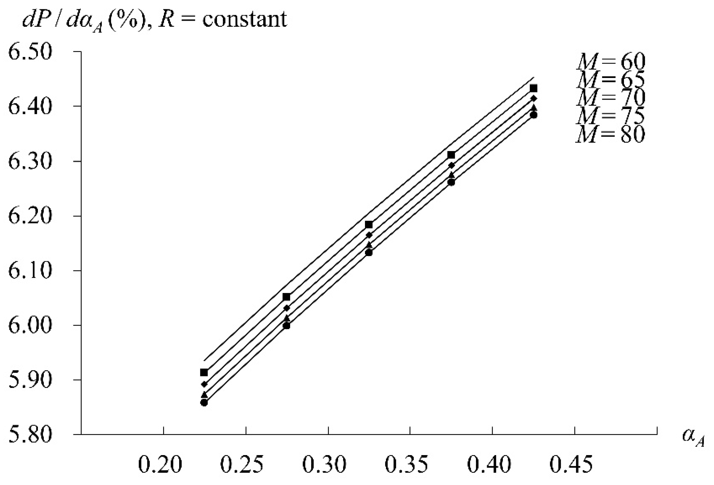
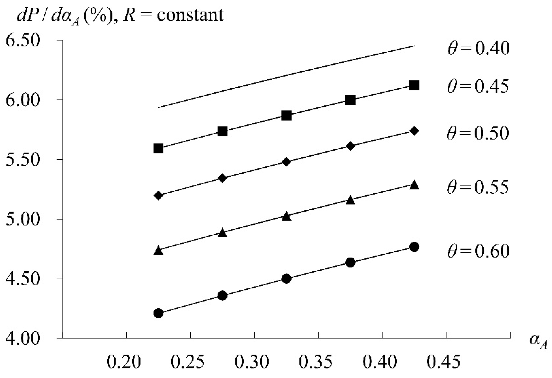
Regarding changes in the other two parameters, namely, the shadow-banking transactions and the government’s purchases of distressed assets, the positive effect of CEO overconfidence on the default risk in the life insurance company’s equity return becomes less significant when the shadow-banking transactions increase (Figure 1), and that when the distressed purchases increase (Figure 2). Our study focuses on the behavioral bias of managerial overconfidence impacting on investment decisions. As the increased shadow-banking transactions conducted by the life insurance company is considered, the company must now provide a return to a lower risk level. Thus, the positive effect of CEO overconfidence on the default risk becomes less significant. The result is understood that shadow insurance could reduce the risk of asset portfolio and thereby improve life insurer performance. Here, we conclude that shadow insurance helps to enhance the survival probabilities. Our conclusion is in large supported by Koijen and Yogo (2016). As an alternative, Figure 2 depicts the relationship between CEO overconfidence and default risk for various levels of the government’s distressed purchases. The same pattern previously stated applies. The life insurance company must now provide a return to a larger capital base and a lower risk level when the distressed purchases increase. Again, this reflects the positive effect of managerial overconfidence on the default risk becomes less significant due to efficiently recapitalized the life insurance company by buying distressed assets from its balance sheet.

Table 3. Responsiveness of liability-side interest margin (guaranteed interest rate) and default risk to CEO overconfidence degree based on Equations (13) and (15) ¹.

	$(R\hspace{0.17em}(\%),\hspace{0.17em}L)$
${\alpha }_A$	(2.25, 285)	(2.50, 307)	(2.75, 323)	(3.00, 334)	(3.25, 341)	(3.50, 345)	(3.75, 347)
	$S$
0.20	88.5708	93.4583	96.7642	98.7667	99.7374	99.9412	99.6359
0.25	91.3848	96.4723	99.9163	102.0058	103.0230	103.2432	102.9342
0.30	94.1872	99.4741	103.0560	105.2324	106.2963	106.5331	106.2208
0.35	96.9780	102.4638	106.1833	108.4467	109.5573	109.8110	109.4958
0.40	99.7572	105.4415	109.2982	111.6485	112.8061	113.0769	112.7592
0.45	102.5250	108.4071	112.4009	114.8381	116.0427	116.3310	116.0110
	$\partial R/\partial {\alpha }_A$
0.20→0.25	-	0.6323	0.5298	0.4216	0.3032	0.1607	-
0.25→0.30	-	0.6068	0.5088	0.4055	0.2926	0.1572	-
0.30→0.35	-	0.5833	0.4894	0.3907	0.2828	0.1539	-
0.35→0.40	-	0.5615	0.4715	0.3769	0.2738	0.1509	-
0.40→0.45	-	0.5412	0.4549	0.3641	0.2654	0.1481	-
	$P$
0.20	0.1117	0.1147	0.1184	0.1224	0.1269	0.1316	0.1366
0.25	0.1147	0.1178	0.1215	0.1257	0.1302	0.1351	0.1401
0.30	0.1177	0.1209	0.1248	0.1290	0.1337	0.1386	0.1437
0.35	0.1208	0.1242	0.1281	0.1324	0.1372	0.1422	0.1474
0.40	0.1240	0.1274	0.1314	0.1359	0.1407	0.1458	0.1511
0.45	0.1272	0.1308	0.1349	0.1394	0.1443	0.1495	0.1549
	$dP/d{\alpha }_A:$ total effect (%),$R_A=$ constant
0.20→0.25	-	6.9302	7.1201	7.2250	7.2593	7.2087	-
0.25→0.30	-	7.0579	7.2425	7.3457	7.3815	7.3361	-
0.30→0.35	-	7.1801	7.3597	7.4613	7.4982	7.4576	-
0.35→0.40	-	7.2972	7.4720	7.5719	7.6099	7.5736	-
0.40→0.45	-	7.4094	7.5797	7.6780	7.7169	7.6846	-

¹ Parameter values, unless stated otherwise, $\delta =0.65$, $\sigma =0.30$, $m=0.10\%$, $\alpha =0.95$, $R_M=5.00\%$, $R_B=4.00\%$, $\beta =0.60$, $M=60$, $\theta =0.40$, and $R_A=5.50\%$. The second-order condition of Equation (11) is consistently confirmed by ${\partial }^{2}S/\partial R^2<0$. The shaded areas represent the values of $S$, $\partial R/\partial {\alpha }_A$, $P$, and $dP/d{\alpha }_A$ with the optimal $R=3.50\%$. The positive indirect effect, $(\partial P/\partial R)(\partial R/\partial {\alpha }_A)>0$, reinforces the positive direct effect, $\partial P/\partial {\alpha }_A>0$.

demonstrates the following two related overconfidence results when the optimal guaranteed rate decisions of the life insurance company are considered. First, the guaranteed rate of the life insurance contract is increased when the CEO overconfidence becomes stronger. As stated earlier, the overconfident CEO overinvests because of overestimating the returns on his/her investments. One way the life insurance company may attempt to augment its total returns is to increase its life insurance policies at an increased guaranteed rate (and thus a decreased interest margin) since overestimating insurer investment returns are an integral part of the contract itself. Second, we show that the default risk in the life insurance company’s equity returns is increased when the CEO overconfidence becomes stronger. The result is understood because overconfidence increases risky investments, directly leading to increasing the default risk. In addition, overconfidence increases the life insurance contracts at an increased guaranteed rate, resulting in increasing cost burden, and hence increasing the default risk in the life insurance company’s equity returns. Therefore, we can argue that CEO overconfidence reinforces marginal cost of issuing policies and thereby results in increasing inefficiency. Our result is in large consistent with an empirical finding of Ho et al. (2016).17 It is important to note that the asset and liability sides of life insurer operations are dichotomized. As mentioned previously, an increase in the CEO overconfidence increases the optimal asset-side interest margin and the default risk of the life insurance company’s equity returns (Table 2) and decreases the optimal liability-side interest margin and increases the default risk (Table 3). Our findings provide evidence that managerial overconfidence from a cognitive bias is more likely to impact insurer spread behavior.

5.3. Bailout Analysis

This subsection considers the following bailout effects on either asset-side or liability-side interest margin management, and then on the default risk in the life insurance company’s equity return and the efficiency gain/loss from CEO overconfidence.

It is necessary to elaborate on the bailout program of buying distressed assets by the government. Toward that end, we compute Equations (16) and (18). The numerical examples provide intuition. The result of $\partial R_A/\partial \theta \hspace{0.17em}<\hspace{0.17em}0$ in Equation (16) observed from the second panel in

Table 4. Responsiveness of asset-side interest margin (asset interest rate) and default risk to buying distressed assets based on Equations (16) and (18) ¹.

	$(R_A(\%),\hspace{0.17em}A)$
$\theta$	(5.50, 300.5)	(5.60, 300)	(5.70, 299)	(5.80, 297)	(5.90, 293)	(6.00, 285)	(6.10, 269)
	$S$
0.40	88.6904	88.7137	88.6163	88.2773	87.4542	85.6613	81.9249
0.45	83.5083	83.5274	83.4345	83.1176	82.3520	80.6871	77.2203
0.50	78.3158	78.3306	78.2424	77.9478	77.2397	75.7035	72.5074
0.55	73.1096	73.1203	73.0368	72.7646	72.1146	70.7077	67.7837
0.60	67.8854	67.8920	67.8133	67.5639	66.9725	65.6959	63.0459
0.65	62.6366	62.6393	62.5657	62.3394	61.8073	60.6624	58.2891
	$\partial R_A/\partial \theta$(%)
0.40→0.45	-	−7.0386	3.7524	9.1416	11.8330	13.1769	-
0.45→0.50	-	−7.5139	4.1159	9.9241	12.8248	14.2724	-
0.50→0.55	-	−8.0377	4.5715	10.8690	14.0137	15.5819	-
0.55→0.60	-	−8.6051	5.1620	12.0380	15.4708	17.1803	-
0.60→0.65	-	−9.1957	5.9607	13.5302	17.3077	19.1845	-
	$P$
0.40	0.1116	0.1111	0.1106	0.1101	0.1098	0.1097	0.1103
0.45	0.1067	0.1062	0.1057	0.1053	0.1050	0.1051	0.1057
0.50	0.1012	0.1008	0.1003	0.1000	0.0997	0.0999	0.1007
0.55	0.0951	0.0947	0.0943	0.0940	0.0938	0.0941	0.0951
0.60	0.0883	0.0879	0.0875	0.0873	0.0872	0.0876	0.0888
0.65	0.0805	0.0802	0.0799	0.0797	0.0797	0.0802	0.0817
	$dP/d\theta :$ total effect
0.40→0.45	-	−0.0973	−0.0972	−0.0965	−0.0954	−0.0934	-
0.45→0.50	-	−0.1084	−0.1081	−0.1073	−0.1060	−0.1038	-
0.50→0.55	-	−0.1212	−0.1208	−0.1199	−0.1184	−0.1158	-
0.55→0.60	-	−0.1361	−0.1356	−0.1345	−0.1328	−0.1298	-
0.60→0.65	-	−0.1534	−0.1528	−0.1515	−0.1495	−0.1460	-

¹ Parameter values, unless stated otherwise, $\delta =0.65$, $\sigma =0.30$, $m=0.10\%$, $\alpha =0.95$, $R_M=5.00\%$, $R_B=4.00\%$, $\beta =0.60$, ${\alpha }_A=0.20$, $M=60$, and $R=2.25\%$. The second-order condition of Equation (10) is consistently confirmed by ${\partial }^{2}S/\partial R_A^2<0$. The shaded areas represent the values of $S$, $\partial R_A/\partial \theta$, $P$, and $dP/d\theta$ with the optimal $R_A=5.60\%$. The positive indirect effect, $(\partial P/\partial R_A)(\partial R_A/\partial \theta )>0$, is insufficient to offset the negative direct effect, $\partial P/\partial \theta <0$.

demonstrates that an increase in buying insurer distressed assets by the government increases the amount of assets at a reduced asset interest rate chosen by the life insurance company. This bailout program results in increasing the life insurance company’s earning revenues since asset demand faced by the company is rate-elastic. The result implies that bailout helps to decrease the life insurance company’s leverage via increasing its core capital ratio, yielding increases to its earning revenues at a reduced interest margin. This explains an important role in discussions of life insurer spread behavior.

Next, the last panel presents the result of $dP/d\theta \hspace{0.17em}<\hspace{0.17em}0$, which can be explained by the direct effect and the indirect effect in Equation (18). The negative direct effect demonstrates decreases in the life insurance company’s default risk due to increases in the buying distressed assets by the government. The result is unambiguous because increases in the buying distressed assets by the government makes the life insurance company’s assets less risky to invest. In response to this, the reduced investment riskiness results in decreasing the default risk in the life insurance company’s equity returns, ceteris paribus. The indirect effect arises when the adjustments of the optimal asset interest rate due to changes in the buying distress assets are explicitly considered. As usual, the sign of this indirect effect is indeterminate. Table 4 provides us with a hunch that the indirect effect evaluated at the optimal $R_A$ is positive. The rationale is that (i) an increase in the buying distressed assets increases the invested assets at a decrease in asset interest rate, as mentioned previously, and then (ii) the default risk is increased due to an increase in the risky asset investment. The indirect effect becomes positive and works against, but insufficiently, the negative direct effect, yielding the result that life insurer default risk reacts negatively to an increase in the bailout program of buying insurer distressed assets. As a result, we argue that buying distressed assets is an appropriate way to recapitalize the life insurance company from the standpoint of financial stability.18

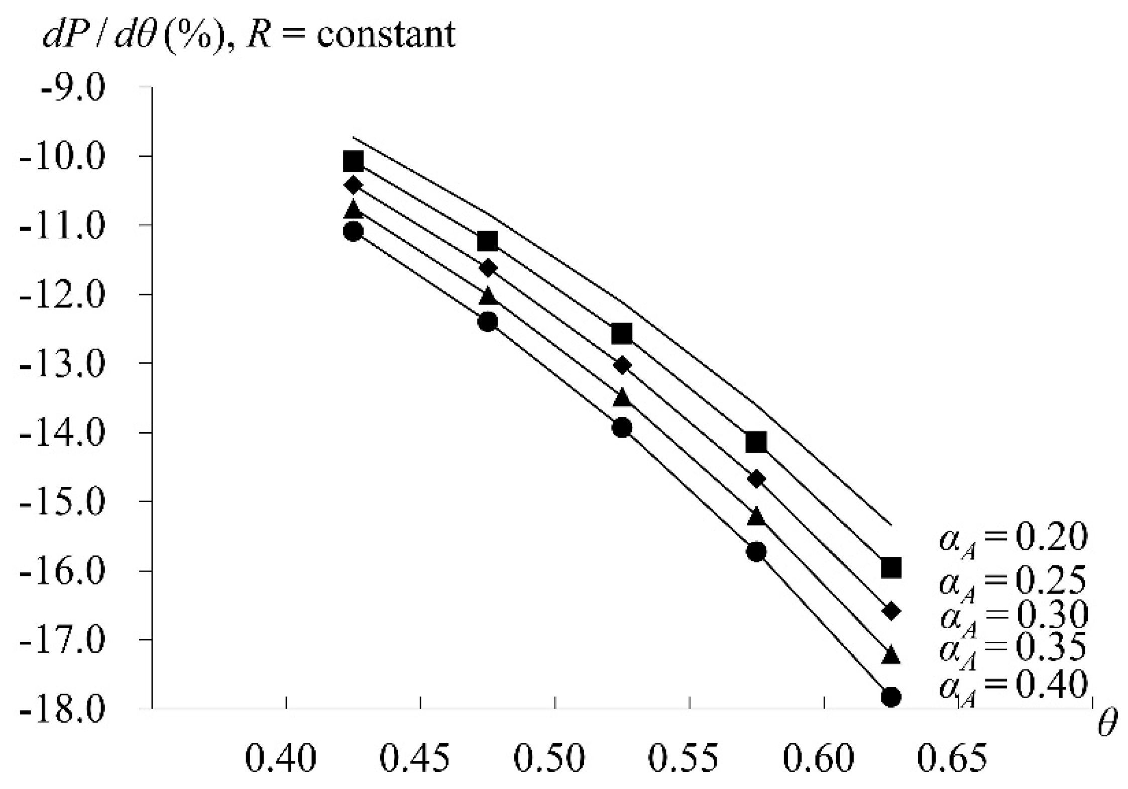
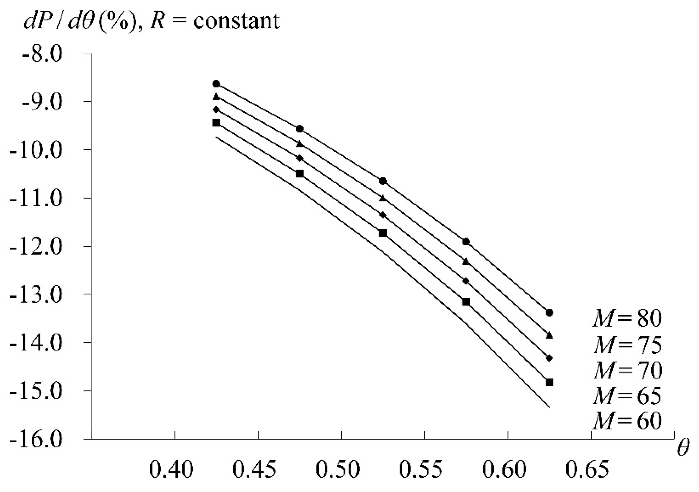
Figure 3 demonstrates the result that the negative effect of the buying of distressed assets by the government on the life insurance company’s default risk becomes more significant when the cognitive bias from CEO overconfidence exacerbates. Not surprisingly, the outcries for more bailouts of the life insurance company with the overconfident CEO tend to be greater. The result is understood because managerial overconfidence induces greater overinvestment and incurs higher investment returns (Malmendier and Tate 2005), and hence increases the effect of the bailout on the decreased default risk. The bailout program of buying distressed assets is an appropriate way to assist the life insurance company. Under the circumstances, CEO overconfidence helps to enhance the survival probabilities as well. Figure 4 suggests that the negative effect of the buying of distressed assets on the life insurance company’s default risk becomes less significant when the life insurance company increasingly gets involved in the shadow-banking transactions. Under the circumstances, shadow insurance incurs higher default risks.

Table 5. Responsiveness of liability-side interest margin (guaranteed interest rate) and default risk to buying distressed assets based on Equations (17) and (19) ¹.

	$(R\hspace{0.17em}(\%),\hspace{0.17em}L)$
$\theta$	(2.25, 285)	(2.50, 307)	(2.75, 323)	(3.00, 334)	(3.25, 341)	(3.50, 345)	(3.75, 347)
	$S$($R_A=$ constant)
0.40	88.5708	93.4583	96.7642	98.7667	99.7374	99.9412	99.6359
0.45	83.3974	87.9120	90.9577	92.7928	93.6696	93.8338	93.5248
0.50	78.2136	82.3549	85.1406	86.8089	87.5925	87.7181	87.4063
0.55	73.0162	76.7837	79.3095	80.8117	81.5032	81.5915	81.2782
0.60	67.8008	71.1936	73.4597	74.7968	75.3976	75.4501	75.1370
0.65	62.5609	65.5777	67.5843	68.7573	69.2693	69.2883	68.9777
	$\partial R/\partial \theta$($R_A=$ constant)
0.40→0.45	-	−1.1789	−0.9982	−0.8111	−0.6126	−0.3884	-
0.45→0.50	-	−1.2706	−1.0740	−0.8702	−0.6536	−0.4079	-
0.50→0.55	-	−1.3788	−1.1628	−0.9386	−0.6998	−0.4273	-
0.55→0.60	-	−1.5087	−1.2684	−1.0187	−0.7518	−0.4452	-
0.60→0.65	-	−1.6686	−1.3968	−1.1137	−0.8102	−0.4585	-
	$P$($R_A=$ constant)
0.40	0.1117	0.1147	0.1184	0.1224	0.1269	0.1316	0.1366
0.45	0.1068	0.1097	0.1133	0.1174	0.1219	0.1267	0.1317
0.50	0.1013	0.1041	0.1077	0.1118	0.1163	0.1211	0.1263
0.55	0.0952	0.0979	0.1014	0.1054	0.1100	0.1149	0.1201
0.60	0.0883	0.0908	0.0942	0.0982	0.1028	0.1077	0.1130
0.65	0.0806	0.0829	0.0861	0.0900	0.0945	0.0995	0.1049
	$dP/d\theta :$ total effect ($R_A=$ constant)
0.40→0.45	-	−0.1144	−0.1152	−0.1138	−0.1106	−0.1058	-
0.45→0.50	-	−0.1267	−0.1281	−0.1270	−0.1238	−0.1186	-
0.50→0.55	-	−0.1409	−0.1432	−0.1424	−0.1393	−0.1338	-
0.55→0.60	-	−0.1573	−0.1608	−0.1607	−0.1577	−0.1519	-
0.60→0.65	-	−0.1764	−0.1814	−0.1822	−0.1795	−0.1734	-

¹ Parameter values, unless stated otherwise, $\delta =0.65$, $\sigma =0.30$, $m=0.10\%$, $\alpha =0.95$, $R_M=5.00\%$, $R_B=4.00\%$, $\beta =0.60$, ${\alpha }_A=0.20$, $M=60$, and $R_A=5.50\%$. The second-order condition of Equation (11) is consistently confirmed by ${\partial }^{2}S/\partial R^2<0$. The shaded areas represent the values of $S$, $\partial R/\partial \theta$, $P$, and $dP/d\theta$ with the optimal $R$. The negative indirect effect, $(\partial P/\partial R)(\partial R/\partial \theta )<0$, reinforces the negative direct effect, $\partial P/\partial \theta <0$.

depicts two effects of government purchases of distressed assets on the optimal guaranteed rate of the life insurance policy, and further on the default risk in the life insurance company’s equity returns when the asset interest rate remained fixed in the dichotomized environment. First, we show that an increase in buying distressed assets by the government decreases the guaranteed rate (and thus increases the interest margin) set by the life insurance company, and therefore leads to less insurance cost burden which increases the equity return. Second, this guaranteed rate decrease also decreases costs which reduces the default risk of equity return (the negative indirect effect in our model). In addition, it is the negative direct effect in our model that a decrease in the default risk due to an increase in buying distressed assets by the government, ceteris paribus. The total negative effect of these two influences can be determined. Overall, the bailout of buying distressed assets induces higher interest margin and incurs lower default risk, thereby contributing to the financial stability.

As mentioned previously, Merkle and Weber (2011) argue that overconfident CEOs who overestimate the value of investment projects due to either mis-calibration or “better-than-effect” bias are expected to overinvest. We further argue that there is an efficiency gain from CEO overconfidence in lieu of CEO rationality due to the life insurance company’s overinvestment (the upper panel in

Table 6. Responsiveness of efficiency gain from CEO overconfidence to buying distressed assets when asset-side interest margin is considered, Equation (20) ¹.

	$(R_A(\%),\hspace{0.17em}A)$
$\theta$	(5.50, 300.5)	(5.60, 300)	(5.70, 299)	(5.80, 297)	(5.90, 293)	(6.00, 285)	(6.10, 269)
	$\Delta E$($R=$ constant)
0.40	382.6842	383.4322	383.6164	382.6658	379.4346	371.6220	354.6120
0.45	365.5638	366.2484	366.3970	365.4670	362.3694	354.9185	338.7295
0.50	348.6239	349.2440	349.3552	348.4429	345.4740	338.3754	322.9901
0.55	331.9120	332.4659	332.5374	331.6391	328.7924	322.0341	307.4298
0.60	315.4932	315.9787	316.0076	315.1183	312.3851	305.9513	292.0981
0.65	299.4595	299.8740	299.8561	298.9692	296.3377	290.2065	277.0639
	$d\Delta E/d\theta :$ total effect ($R=$ constant)
0.40→0.45	-	−344.2025	−344.3187	−344.8459	−345.1266	−344.3650	-
0.45→0.50	-	−340.6029	−340.7746	−341.4050	−341.8812	−341.4956	-
0.50→0.55	-	−336.0606	−336.3045	−337.0674	−337.7932	−337.8868	-
0.55→0.60	-	−330.2196	−330.5597	−331.4968	−332.5493	−333.2681	-
0.60→0.65	-	−322.5414	−323.0135	−324.1863	−325.6788	−327.2374	-

¹ Parameter values, unless stated otherwise, $\delta =0.65$, $\sigma =0.30$, $m=0.10\%$, $\alpha =0.95$, $R_M=5.00\%$, $R_B=4.00\%$, $\beta =0.60$, ${\alpha }_A=0.20$, $M=60$, and $R=2.25\%$. The shaded areas represent the values of $\Delta E$ and $d\Delta E/d\theta$ with the optimal $R_A$. The negative indirect effect, $(\partial \Delta E/\partial R_A)(\partial R_A/\partial \theta )<0$, reinforces the negative direct effect, $\partial \Delta E/\partial \theta <0$.

). This is because the life insurance company optimally determines the insurer interest margin by exercising some monopoly power in the asset market. Overinvestment returns efficiently allow the life insurance company to have the equity maximization at the optimal interest margin. However, an increase in the buying distressed assets by the government decreases the efficiency gain from CEO overconfidence in the life insurance company’s overinvestment (the lower panel in Table 6). Intuitively, when the life insurer company decides to participate in the bailout program of buying distressed assets, the bailout may generate an adverse signal that the life insurance company is expected to have high future losses. Under the circumstances, the overconfident CEO with a less cognitive bias reveals less overinvestment due to the adverse signal realization, which reduces the efficiency gain from CEO overconfidence. As a result, CEO overconfidence induces higher efficiency gain from insurer overinvestment but reduces the efficiency gain when the bailout of buying distressed assets is increased.

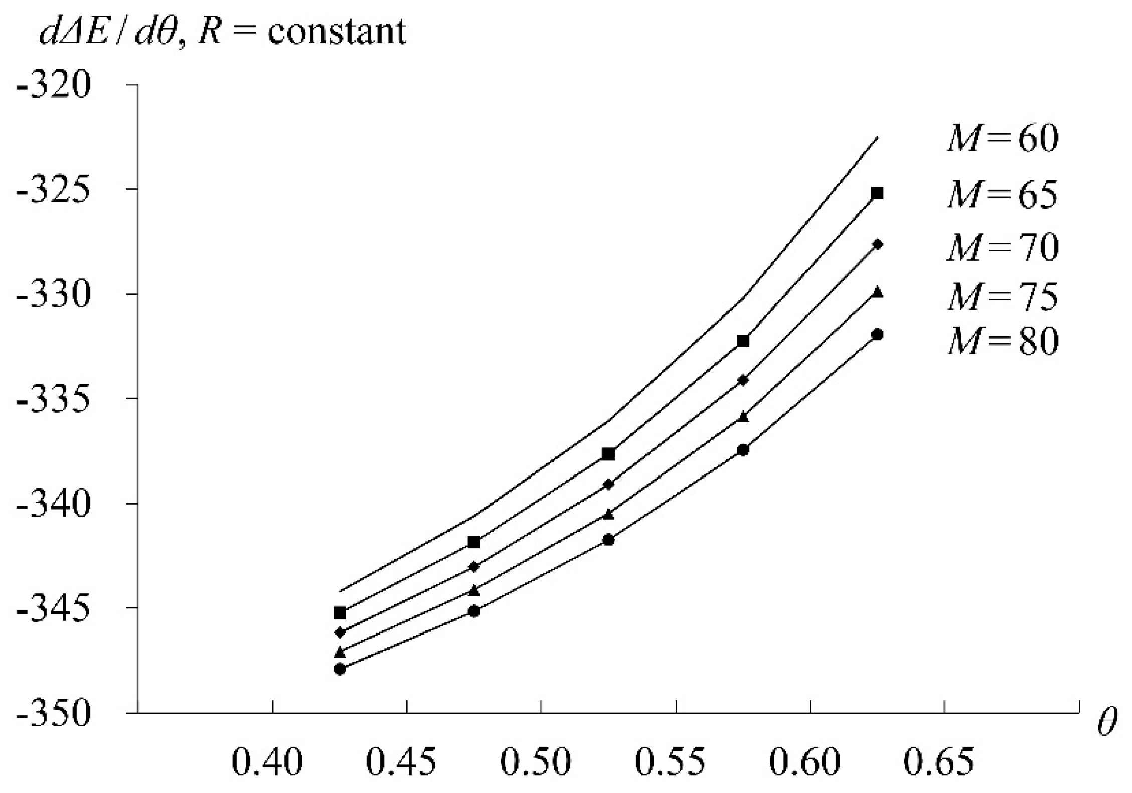
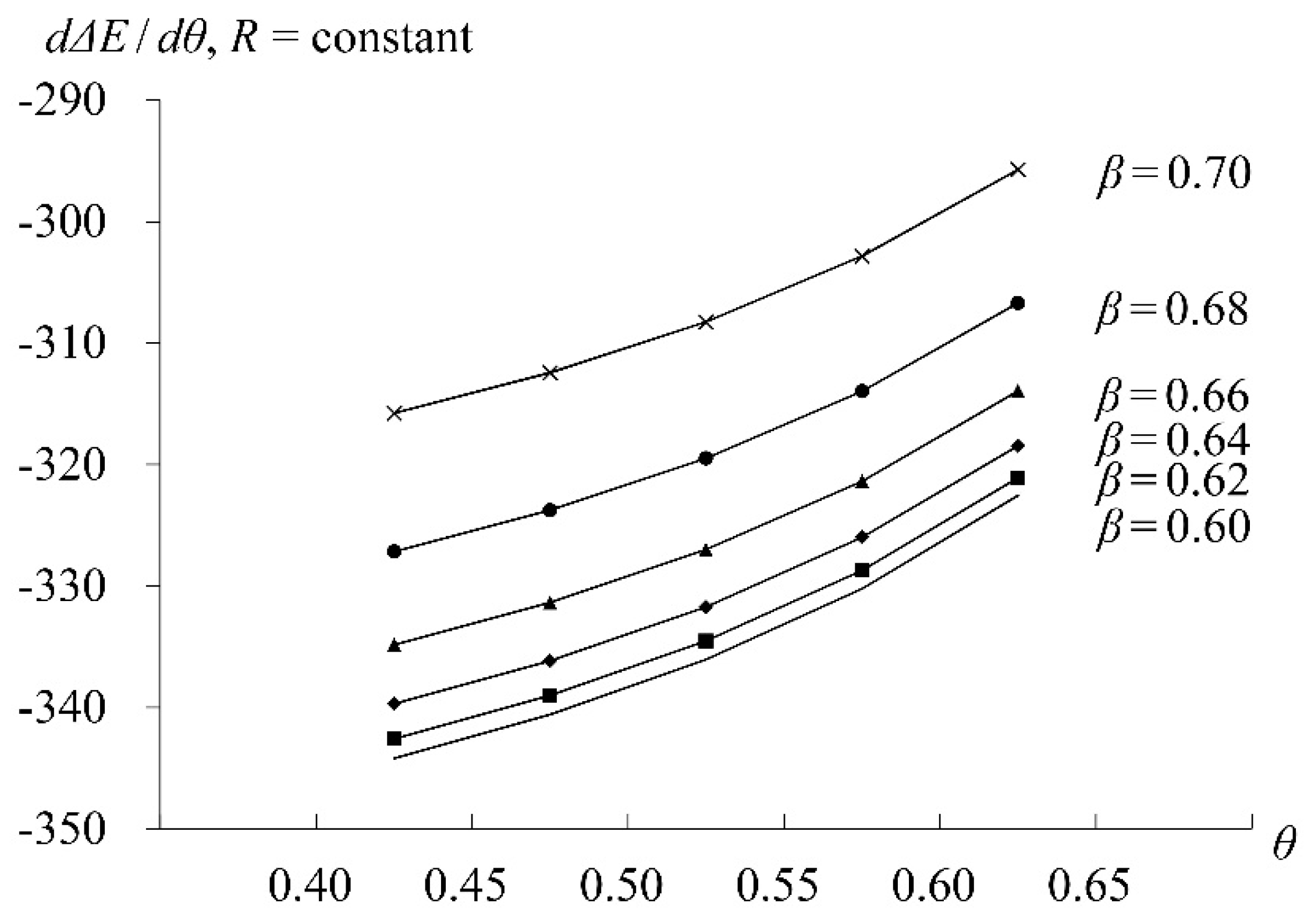
Figure 5 demonstrates that the negative effect of buying distressed assets on the efficiency gain from CEO overconfidence is increased when the shadow-banking activities involved by the life insurance company increase. If we can argue that buying distressed assets, reducing an efficiency gain from CEO overconfidence, is an appropriate way to recapitalize the life insurance company, an increase in the shadow insurance reinforces the appropriateness. Figure 6 states that the negative effect of buying distressed assets on the efficiency gain from CEO overconfidence is decreased when the barrier ratio in the equity valuation increases. The same pattern as before applies. The government is interested in CEO overconfidence as long as the risk of a premature default to the equity valuation of the life insurance company is decreased.

Table 7. Responsiveness of efficiency gain from CEO overconfidence to buying distressed assets when liability-side interest margin is considered, Equation (21) ¹.

	$(R\hspace{0.17em}(\%),\hspace{0.17em}L)$
$\theta$	(2.25, 285)	(2.50, 307)	(2.75, 323)	(3.00, 334)	(3.25, 341)	(3.50, 345)	(3.75, 347)
	$\Delta E$($R_A=$ constant)
0.40	382.1271	399.4593	409.0159	412.3793	411.0198	406.2966	399.4606
0.45	365.0342	381.1930	389.9318	392.7723	391.1249	386.2899	379.4602
0.50	348.1212	363.1163	371.0382	373.3498	371.4041	366.4444	359.6067
0.55	331.4355	345.2799	352.3864	354.1622	351.9052	346.8041	339.9401
0.60	315.0418	327.7539	334.0481	335.2795	332.6946	327.4307	320.5169
0.65	299.0321	310.6385	316.1261	316.8026	313.8683	308.4133	301.4180
	$d\Delta E/d\theta :$ total effect ($R_A=$ constant)
0.40→0.45	-	−447.0598	−419.8383	−403.0517	−394.5667	−392.7941	-
0.45→0.50	-	−443.6601	−415.4157	−398.3368	−390.1077	−389.0221	-
0.50→0.55	-	−439.4267	−409.8815	−392.4324	−384.5324	−384.3285	-
0.55→0.60	-	−434.0668	−402.8217	−384.8895	−377.4238	−378.3831	-
0.60→0.65	-	−427.1525	−393.6093	−375.0231	−368.1493	−370.6963	-

¹ Parameter values, unless stated otherwise, $\delta =0.65$, $\sigma =0.30$, $m=0.10\%$, $\alpha =0.95$, $R_M=5.00\%$, $R_B=4.00\%$, $\beta =0.60$, ${\alpha }_A=0.20$, $M=60$, and $R_A=5.50\%$. The shaded areas represent the values of $\Delta E$ and $d\Delta E/d\theta$ with the optimal $R$. The positive indirect effect, $(\partial \Delta E/\partial R)(\partial R/\partial \theta )>0$, is insufficient to offset the negative direct effect, $\partial \Delta E/\partial \theta <0$.

demonstrates the case that the optimal guaranteed interest rate of the life insurance policy is determined in a non-simultaneous environment where the optimal asset interest rate chosen by the life insurance company remains constant. We conclude that the life insurance company with the overconfident CEO is more likely to increase efficiency gain from overinvestment than life insurance companies with rational CEO. However, the efficiency gains from CEO overconfidence due to overinvestment is reduced when the bailout program of buying distressed assets increases. The same interpretation as before applies. Note that an increase in the bailout decreases the life insurance policies at a reduced guaranteed rate, yielding increases to the efficiency gain due to overinvestment with CEO overconfidence. This indirect effect is insufficient to offset the negative direct effect to give an overall negative effect of buying distressed assets on the efficiency gain from CEO overconfidence.

6. Conclusions

Guided by the existing theories, this paper theoretically develops the impact of managerial overconfidence on insurer interest margin, and default risk at various levels of shadow-banking transactions conducted by the life insurance company. This paper also investigates the effect of bailout on insurer interest margin, default risk, and efficiency gain/loss from CEO overconfidence at various levels of shadow-banking involvement.

Our two main results are as follows. First, CEO overconfidence raises the default risk in the life insurance company’s equity returns regardless of whether asset-side or liability-side interest margin is determined. Shadow-banking activities involved by the life insurance company attenuate the unfavorable effect. Buying distressed assets by the government weakens the effect as well. Second, government bailouts help to reduce the default risk in the life insurance company’s equity returns regardless of whether asset-side or liability-side interest margin is determined. However, government bailouts reduce the efficiency gain from CEO overconfidence. If the case is that buying distressed assets is an appropriate way to recapitalize the life insurance company, an increase in the shadow-banking involvement reinforces the appropriateness.

One caveat that should be stressed is that this analysis focuses only on a cognitive bias in which managerial overconfidence impacts insurer investment decisions and does not deal with the many other important areas of the life insurance policies. For example, issues such as managerial overconfidence affecting the guaranteed interest rate and the participation level of the profit-sharing life insurance policies are not considered. While there are significant issues, they can be perhaps understood only when the underlying economic link between life insurance policy issuance and market demand status is made clear. Such concerns are beyond the scope of this research and so are not addressed here. What this research does demonstrate, however, is the important role played by managerial overconfidence in affecting insurer investment decisions and further insurer bankruptcy prediction.

References

1. Adams, Renee B., and Daniel Ferreira. 2007. A theory of friendly boards. Journal of Finance 62: 217–50. [Google Scholar] [CrossRef]
2. Adrian, Tobias, and Hyun Song Shin. 2009. The shadow banking system: Implications for financial regulation. Financial Stability Review, Banque de France 13: 1–10. Available online: https://publications.banque-france.fr/sites/default/files/medias/documents/financial-stability-review-13_2009-09.pdf (accessed on 23 February 2019).
3. Adrian, Tobias, and Mark M. Westerfield. 2009. Disagreement and learning in a dynamic contracting model. Review of Financial Studies 10: 3873–906. [Google Scholar] [CrossRef]
4. Alicke, Mark D. 1985. Global self-evaluation as determined by the desirability and controllability of trait adjectives. Journal of Personality and Social Psychology 49: 1621–30. [Google Scholar] [CrossRef]
5. Barnes, Michelle L. 2016. Did life Insurers Benefit from TARP or Regulatory Forbearance during the Financial Crisis of 2008–2009? FRB of Boston Working Paper No. 16-24. Available online: https://ssrn.com/abstract=2917098 (accessed on 29 January 2019).
6. Ben-David, Itzhak, John R. Graham, and Campbell R. Harvey. 2013. Managerial miscalibration. Quarterly Journal of Economics 128: 1547–84. [Google Scholar] [CrossRef]
7. Berry-Stölzle, Thomas R., Gregory P. Nini, and Sabine Wende. 2014. External financing in the life insurance industry: Evidence from the financial crisis. Journal of Risk and Insurance 81: 529–62. [Google Scholar] [CrossRef]
8. Berry-Stölzle, Thomas R., Evan M. Eastman, and Jianren Xu. 2018. CEO overconfidence and earnings management: Evidence from property-liability insurers’ loss reserves. North American Actuarial Journal 22: 380–404. [Google Scholar] [CrossRef]
9. Breitenfellner, Bastian, and Niklas Wagner. 2010. Government intervention in response to the subprime financial crisis: The good into the pot, the bad into the crop. International Review of Financial Analysis 19: 289–97. [Google Scholar] [CrossRef]
10. Briys, Eric, and François de Varenne. 1994. Life insurance in a contingent claim framework: Pricing and regulatory implications. Geneva Papers on Risk and Insurance Theory 19: 53–72. [Google Scholar] [CrossRef]
11. Brockman, Paul, and H. J. Turtle. 2003. A barrier option framework for corporate security valuation. Journal of Financial Economics 67: 511–29. [Google Scholar] [CrossRef]
12. Calomiris, Charles W., and Urooj Khan. 2015. An assessment of TARP assistance to financial institutions. Journal of Economic Perspectives 29: 53–80. [Google Scholar] [CrossRef]
13. Campbell, T. Colin, Michael Gallmeyer, Shane A. Johnson, Jessica Rutherford, and Brooke W. Stanley. 2011. CEO optimism and forced turnover. Journal of Financial Economics 101: 695–712. [Google Scholar] [CrossRef]
14. Ceci, Claudia, Katia Colaneri, and Alessandra Cretarola. 2017. Unit-linked life insurance policies: Optimal hedging in partially observable market models. Insurance: Mathematics and Economics 76: 149–63. [Google Scholar] [CrossRef]
15. Chen, An, and Michael Suchanecki. 2007. Default risk, bankruptcy procedures and the market value of life insurance liabilities. Insurance: Mathematics and Economics 40: 231–55. [Google Scholar] [CrossRef]
16. Choi, Paul Moon Sub, Chune Young Chung, and Chang Liu. 2018. Self-attribution of overconfident CEOs and asymmetric investment-cash flow sensitivity. North American Journal of Economics and Finance 46: 1–14. [Google Scholar] [CrossRef]
17. Dyreng, Scott D., Michelle Hanlon, and Edward L. Maydew. 2010. The effects of executives on corporate tax avoidance. The Accounting Review 85: 1163–89. [Google Scholar] [CrossRef]
18. Ergungor, Ozgur Emre. 2005. The profitability of bank-borrower relationships. Journal of Financial Intermediation 14: 485–512. [Google Scholar] [CrossRef]
19. Fahlenbrach, Rüdiger, and René M. Stulz. 2011. Bank CEO incentives and the credit crisis. Journal of Financial Economics 99: 11–26. [Google Scholar] [CrossRef] [Green Version]
20. Giat, Yahel, Steve T. Hackman, and Ajay Subramanian. 2009. Investment under uncertainty, heterogeneous beliefs, and agency conflicts. Review of Financial Studies 23: 1360–404. [Google Scholar] [CrossRef]
21. Goel, Anand M., and Anjan V. Thakor. 2008. Overconfidence, CEO selection, and corporate governance. Journal of Finance 63: 2737–84. [Google Scholar] [CrossRef]
22. Gómez, Fabiana, and Jorge Ponce. 2018. Systemic risk and insurance regulation. Risks 6: 74. [Google Scholar] [CrossRef]
23. Gorton, Gary, and Andrew Metrick. 2010. Regulating the shadow banking system. Brookings Papers on Economic Activity 2010: 261–97. [Google Scholar] [CrossRef]
24. Grosen, Anders, and Peter Løchte Jørgensen. 2002. Life insurance liabilities at market values: An analysis of insolvency risk, bonus policy, and regulatory intervention rules in a barrier option framework. Journal of Risk and Insurance 69: 63–91. [Google Scholar] [CrossRef]
25. Harrington, Scott E. 2009. The financial crisis, systemic risk, and the future of insurance regulation. Journal of Risk and Insurance 76: 785–819. [Google Scholar] [CrossRef]
26. Heaton, James B. 2002. Managerial optimism and corporate finance. Financial Management 31: 33–45. [Google Scholar] [CrossRef]
27. Hirshleifer, Dice, and Guo Ying Luo. 2001. On the survival of overconfident traders in a competitive securities market. Journal of Financial Markets 4: 73–84. [Google Scholar] [CrossRef] [Green Version]
28. Ho, Po-Hsin, Chia-Wei Huang, Chih-Yung Lin, and Ju-Fang Yen. 2016. CEO overconfidence and financial crisis: Evidence from bank lending and leverage. Journal of Financial Economics 120: 194–209. [Google Scholar] [CrossRef]
29. Hong, Jimin, and S. Hun Seog. 2018. Life insurance settlement and the monopolistic insurance market. Insurance: Mathematics and Economics 81: 36–50. [Google Scholar] [CrossRef]
30. Hoshi, Takeo, and Anil K. Kashyap. 2010. Will the US bank recapitalization succeed? Eight lessons from Japan. Journal of Financial Economics 97: 398–417. [Google Scholar] [CrossRef]
31. Hsieh, Tien-Shih, Jean C. Bedard, and Karla M. Johnstone. 2014. CEO overconfidence and earnings management during shifting regulatory regimes. Journal of Business Finance & Accounting 41: 1243–68. [Google Scholar] [CrossRef]
32. Insurance Europe. 2014. Why Insurers Differ from Banks. November 5, Brussels: Insurance Europe, Available online: http://www.insuranceeurope.eu/sites/default/files/attachments/Why%20insurers%20differ%20from%20banks.pdf (accessed on 29 January 2019).
33. Insurance Europe and Oliver Wyman. 2013. Funding the Future: Insurers’ Role as Institutional Investors. Available online: www.insuranceeurope.eu (accessed on 3 March 2019).
34. Irresberger, Felix, and Ying Peng. 2017. Shadow Insurance Usage and Capital Management in Life Insurance Groups. Fox School of Business Research Paper No. 16-022. Available online: https://ssrn.com/abstract=2754489 (accessed on 29 January 2019).
35. Jeffers, Esther, and Claudia Baicu. 2013. The Interconnections Between the Shadow Banking System and the Regular Banking System: Evidence from the Euro Area. CITYPERC Working Paper Series 2013-07; London, UK: Department of International Politics, City University London, Available online: http://openaccess.city.ac.uk/2119/1/CITYPERC-WPS-2013_07.pdf (accessed on 23 February 2019).
36. Kim, Kyeonghee, J. Tyler Leverty, and Joan T. Schmit. 2017. The effect of investment advisors in the life insurance industry. Working Paper, University of Wisconsin-Madison. Available online: https://bus.wisc.edu/-/media/bus/knowledge-expertise/academic-departments/asrmi/events/2017-2018/kyeongheekim_jobmarketpaper.pdf?la=en (accessed on 23 February 2019).
37. Koijen, Ralph S. J., and Motohiro Yogo. 2016. Shadow insurance. Econometrica 84: 1265–87. [Google Scholar] [CrossRef]
38. Li, Xuelian, and Jyh-Horng Lin. 2016. Shadow-banking entrusted loan management, deposit insurance premium, and capital regulation. International Review of Economics and Finance 41: 98–109. [Google Scholar] [CrossRef]
39. Lin, Jyh-Jiuan, Chuen-Ping Chang, and Shi Chen. 2018. How does distress acquisition incentivized by government purchases of distressed loans affect bank default risk? Risks 6: 39. [Google Scholar] [CrossRef]
40. Ma, Yueran. 2014. Bank CEO optimism and the financial crisis. Unpublished Working Paper, Harvard University, Cambridge, MA, USA. Available online: http://scholar.harvard.edu/files/yueranma/files/bankoptimism_0.pdf (accessed on 29 January 2019).
41. Malmendier, Ulrike, and Geoffrey Tate. 2005. CEO overconfidence and corporate investment. Journal of Finance 60: 2661–700. [Google Scholar] [CrossRef]
42. Merkle, Christoph, and Martin Weber. 2011. True overconfidence: The inability of rational information processing to account for apparent overconfidence. Organizational Behavior and Human Decision Processes 116: 262–71. [Google Scholar] [CrossRef]
43. Moore, Don A., and Paul J. Healy. 2008. The trouble with overconfidence. Psychological Review 115: 502–17. [Google Scholar] [CrossRef] [PubMed]
44. Niehaus, Greg. 2014. Managing Capital and Insolvency Risk via Internal Capital Market Transactions: The case of Life Insurers. Available online: https://ssrn.com/abstract=2429024 (accessed on 29 January 2019).
45. Plantin, Guillaume. 2015. Shadow banking and bank capital regulation. Review of Financial Studies 28: 146–75. [Google Scholar] [CrossRef]
46. Pozsar, Zoltan. 2008. The Rise and Fall of the Shadow Banking System. Regional Financial Review 44: 13–25. Available online: http://wisburg.com/wp-content/uploads/2017/04/sbs.pdf (accessed on 23 February 2019).
47. Pozsar, Zoltan, Tobias Adrian, Adam Ashcraft, and Hayley Boesky. 2013. Shadow Banking. Federal Reserve Bank of New York Economic Policy Review 19: 1–16. Available online: https://www.newyorkfed.org/medialibrary/media/research/epr/2013/0713adri.pdf (accessed on 23 February 2019).
48. Ronn, Ehud I., and Avinash K. Verma. 1986. Pricing risk-adjusted deposit insurance: An option-based model. Journal of Finance 41: 871–95. [Google Scholar] [CrossRef]
49. Slovin, Myron B., and Marie Elizabeth Sushka. 1983. A model of the commercial loan rate. Journal of Finance 38: 1583–96. [Google Scholar] [CrossRef]
50. Thimann, Christian. 2014. How Insurers Differ from Banks: A Primer in Systemic Regulation. SRC Special Paper No 3. Available online: https://ssrn.com/abstract=2502458 (accessed on 29 January 2019).
51. Tsagkanos, G. Athanasios, and Costas Siriopoulos. 2015. Stock markets and industrial production in north and south of Euro-zone: Asymmetric effects via threshold cointegration approach. Journal of Economic Asymmetries 12: 162–72. [Google Scholar] [CrossRef]
1
The assistance from the Troubled Asset Relief Program (TARP) changed after the 2008 election. Attention focused on evaluating the financial circumstances of particular large institutions whose financing structure problematic. TARP was created to meet the needs for what the Treasury termed “exceptional assistance” by three large institutions: AIG, Citigroup, and Bank of America because they were “too big to fail” (Calomiris and Khan 2015).
2
Hereafter, the terms “insurer” or “life insurer” refer to “life insurance company”.
3
The insurance industry is one of the largest institutional investors in Europe (Insurance Europe and Oliver Wyman 2013).
4
For example, see Briys and de Varenne (1994); Grosen and Jørgensen (2002); Chen and Suchanecki (2007); and Ceci et al. (2017). The issue of life insurance settlement presented by Hong and Seog (2018) is an exception.
5
We thank an anonymous reviewer whose detailed comments helped us to avoiding ignoring the potential argument of “tone at the top” in the literature.
6
The investment advisors are common in the life insurance industry and potentially give more thought to how CEO overconfidence translates to investment decisions. We would like to thank an anonymous reviewer for pointing this possibility out to us.
7
Shadow banking is huge globally, accounting for about 25% of total money transfers between savers and borrowers worldwide. Overviews of the shadow banking system are provided by Pozsar (2008), who catalogues different types of shadow banks and describes the asset and funding flows within the system, and Adrian and Shin (2009), who focus on the role of security brokers and dealers in the system and discuss implications for financial regulation. Gorton and Metrick (2010), and Pozsar et al. (2013) document that the growth of shadow banking has been largely driven by regulatory arbitrage. Plantin (2015) argues that tightening capital requirements may increase shadow banking activities and make banks that not willing to incur adverse selection costs very safe; alternatively, relaxing capital requirements may bring shadow banking activities back in the spotlight of regulation. However, Pozsar et al. (2013) and Jeffers and Baicu (2013) indicate that the interconnections between regular banking and shadow banking activities have negative consequences on financial stability.
8
If we think that CEO labor markets are efficient, we would expect certain types of firms to hire overconfident CEOs and other firms to hire non-overconfident CEOs. Prior studies deal with this. endogeneity (Ho et al. 2016; Berry-Stölzle et al. 2018). Since this perspective can be explored applying the exact same assumption of α A > 0 , we believe this issue have no impact on the findings in our study. Another potential issue is that α A is assumed to be independent to the expected return ( 1 + R A ) A . This assumption ignores the presence of asymmetric adjustment behavior and regime switch under financial turmoil. See Tsagkanos and Siriopoulos (2015) for an analysis on asymmetric effects via threshold cointegration approach.
9
Mis-calibration and the “better-than-average” bias are known to structure CEO overconfidence (e.g., see Merkle and Weber 2011). Miscalibration implies the excessive belief in one’s precision, while the “better-than-average” bias implies the tendency to place one’s performance and ability as superior to an average peer (e.g., see Moore and Healy 2008; Choi et al. 2018).
10
Malmendier and Tate (2005) develop a CEO overconfidence behavior of a firm with exactly this structure. In addition, our model is limited to the case of overconfidence behavior with overestimated of future payoffs on investments. However, this model is also applicable to the case of underestimated future returns when α A < 0 . Since our results show that all the effects of α A are monotonic, our results can be adapted to situations where α A is less than zero and within a reasonable range. Adding this complexity affects none of qualitative comparative static results in the paper. The condition that α A < 0 may be used to analyze the assumption of under-confident CEOs. See, for example, Campbell et al. (2011) include a spectrum of confidence (they refer to it as “optimism”).
11
As pointed out by Barnes (2016) in previous section, the 2008 financial crisis has witnessed large government bailouts of several life insurance companies worldwide, the most notable being AIG.
12
The goal of Li and Lin (2016) is to explore the role played by bank spread management under capital regulation in the commercial lending and shadow-banking entrusted lending activities. The role played by the trustee in Li and Lin (2016) is assumed to be a bank. This assumption is applicable to a case of a life insurance company permitted by regulation.
13
Koijen and Yogo (2016) investigate the issue that life insurance companies use reinsurance to move liabilities from regulated companies that sell policies to shadow reinsures. What distinguishes our work from this literature is our focus on the question whether a life insurance company benefits or gets hurt from shadow banking activities on its asset portfolio, specifically including loans and/or entrusted loans.
14
We simplify our discussion by assuming a zero rebate upon failure in the formula for the down-and-out call option in the model.
15
Slovin and Sushka (1983) develop a model of the commercial loan rate where the asset and liability sides of bank operations are assumed to be dichotomized. We employ their conceptual approach to model the optimal solutions of CEO overconfidence issues.
16
Berry-Stölzle et al. (2018) examine the relation between CEO overconfidence and earnings management in the U.S. property-ability insurance industry. The authors find that overconfident managers overestimate the returns on their investment projects and underestimate losses, implicitly resulting in increasing the default risk of the insurance companies.
17
Ho et al. (2016) find that overconfident banks experience more severe worsening of stock return performance, along with greater increases in default risk. We argue that their finding may be applicable to life insurance companies since bank and insurance company can be broadly classified as a financial institution.
18
Hoshi and Kashyap (2010) also conclude the result for distressed banks.
Figure 1. Responsiveness of default risk to overconfidence degree at various levels of shadow-banking transaction based on Equation (14). Parameter values, unless stated otherwise, δ = 0.65 , σ = 0.30 , m = 0.10 % , α = 0.95 , R M = 5.00 % , R B = 4.00 % , β = 0.60 , θ = 0.40 , and R = 2.25 % . All results are valued at the optimal R A of 5.60%. The negative indirect effect, ( P / R A ) ( R A / α A ) < 0 , is consistently insufficient to offset the positive direct effect, P / α A > 0 at various levels of shadow-banking transaction.
Risks 07 00028 g001
Figure 2. Responsiveness of default risk to overconfidence degree at various levels of buying distressed assets by the government based on Equation (14). Parameter values, unless stated otherwise, δ = 0.65 , σ = 0.30 , m = 0.10 % , α = 0.95 , R M = 5.00 % , R B = 4.00 % , β = 0.60 , M = 60 , and R = 2.25 % . All results are valued at the optimal R A of 5.60%. The negative indirect effect, ( P / R A ) ( R A / α A ) < 0 , is insufficient to offset the positive direct effect, P / α A > 0 .
Risks 07 00028 g002
Figure 3. Responsiveness of default risk to buying distressed assets at various levels of CEO overconfidence based on Equation (18). Parameter values, unless stated otherwise, δ = 0.65 , σ = 0.30 , m = 0.10 % , α = 0.95 , R M = 5.00 % , R B = 4.00 % , β = 0.60 , M = 60 , and R = 2.25 % . All results are valued at the optimal R A of 5.60%. The positive indirect effect, ( P / R A ) ( R A / θ ) > 0 , is consistently insufficient to offset the negative direct effect, P / θ < 0 at various levels of CEO overconfidence.
Risks 07 00028 g003
Figure 4. Responsiveness of default risk to buying distressed assets at various levels of shadow-banking transaction based on Equation (18). Parameter values, unless stated otherwise, δ = 0.65 , σ = 0.30 , m = 0.10 % , α = 0.95 , R M = 5.00 % , R B = 4.00 % , β = 0.60 , α A = 0.20 , and R = 2.25 % . All results are valued at the optimal R A of 5.60%. The positive indirect effect, ( P / R A ) ( R A / θ ) > 0 , is consistently insufficient to offset the negative direct effect, P / θ < 0 at various levels of shadow-banking transaction.
Risks 07 00028 g004
Figure 5. Responsiveness of efficiency gain to buying distressed assets at various levels of shadow-banking transaction based on Equation (20). All results are valued at the optimal R A of 5.60%. The negative indirect effect, ( Δ E / R A ) ( R A / θ ) < 0 , consistently reinforces the negative direct effect, Δ E / θ < 0 at various levels of shadow-banking transaction.
Risks 07 00028 g005
Figure 6. Responsiveness of efficiency gain to buying distressed assets at various levels of barrier based on Equation (20). All results are valued at the optimal R A of 5.60%. The negative indirect effect, ( Δ E / R A ) ( R A / θ ) < 0 , consistently reinforces the negative direct effect, Δ E / θ < 0 at various levels of shadow-banking transaction.
Risks 07 00028 g006