Article

The W,Z/ν,δ Paradigm for the First Passage of Strong Markov Processes without Positive Jumps

1
Laboratoire de Mathématiques Appliquées, Université de Pau, 64012 Pau, France
2
Department of Mathematics, University of Osijek, 31000 Osijek, Croatia
3
Department of Statistics, Middle East Technical University, Ankara 06800, Turkey
*
Author to whom correspondence should be addressed.
Risks 2019, 7(1), 18; https://doi.org/10.3390/risks7010018
Submission received: 21 November 2018 / Revised: 31 January 2019 / Accepted: 13 February 2019 / Published: 19 February 2019

Abstract

:
As is well-known, the benefit of restricting Lévy processes without positive jumps is the “ W , Z scale functions paradigm”, by which the knowledge of the scale functions W , Z extends immediately to other risk control problems. The same is true largely for strong Markov processes X t , with the notable distinctions that (a) it is more convenient to use as “basis” differential exit functions ν , δ , and that (b) it is not yet known how to compute ν , δ or W , Z beyond the Lévy, diffusion, and a few other cases. The unifying framework outlined in this paper suggests, however, via an example that the spectrally negative Markov and Lévy cases are very similar (except for the level of work involved in computing the basic functions ν , δ ). We illustrate the potential of the unified framework by introducing a new objective (33) for the optimization of dividends, inspired by the de Finetti problem of maximizing expected discounted cumulative dividends until ruin, where we replace ruin with an optimally chosen Azema-Yor/generalized draw-down/regret/trailing stopping time. This is defined as a hitting time of the “draw-down” process Y t = sup 0 s t X s X t obtained by reflecting X t at its maximum. This new variational problem has been solved in a parallel paper.

1. A Brief Review of First Passage Theory for Strong Markov Processes without Positive Jumps and Their Draw-Downs

Motivation. First passage times intervene in the control of reserves/risk processes. The rough idea is that when below low levels a, the reserves should be replenished at some cost, and when above high levels b, the reserves should be invested to yield dividends—see for example Albrecher and Asmussen (2010). There is a wide variety of first passage control problems (involving absorption, reflection and other boundary mechanisms), and it has been known for a long while that these problems are simpler in the “completely asymmetric” case when all jumps go in the same direction. In recent years it has become clearer that most first passage problems can be reduced to the two basic problems of going up before down, or vice versa, and that their answers may usually be ergonomically expressed in terms of two basic “scale functions” W , Z (Albrecher et al. (2016); Avram et al. (2004, 2007, 2015, 2017a, 2017b, 2018a, 2018b); Avram and Zhou (2017); Bertoin (1997); Ivanovs and Palmowski (2012); Kyprianou (2014); Landriault et al. (2017b); Li et al. (2017); Li and Zhou (2018); Suprun (1976)). The proofs require typically not much more than the strong Markov property; it is natural, therefore, to develop extensions to strong Markov processes. This has been achieved already in particular spectrally negative cases such as random walks Avram and Vidmar (2017), Markov additive processes Ivanovs and Palmowski (2012), Lévy processes with Ω state-dependent killing Ivanovs and Palmowski (2012), certain Lévy processes with state-dependent drift Czarna et al. (2017), and is in fact possible in general. However, characterizing the functions W , Z is still an open problem, even for simple classic processes such as the Ornstein-Uhlenbeck and the Feller branching diffusion with jumps.
Let X t denote a one-dimensional strong Markov process without positive jumps, defined on a filtered probability space ( Ω , { F t } t 0 , P ) . Denote its first passage times above and below by
T b , + = T b , + ( X ) = inf { t 0 : X t > b } , T a , = T a , ( X ) = inf { t 0 : X t < a } ,
with inf = + .
Recall that first passage theory for diffusions and spectrally negative or spectrally positive Lévy processes is considerably simpler than that for processes which may jump both ways. For these two families, a large variety of first passage problems may be reduced to the computation of two monotone “scale functions” W , Z (by simple arguments such as the strong Markov property). See Albrecher et al. (2016); Avram et al. (2004, 2007, 2015, 2017a, 2018a); Avram and Zhou (2017); Bertoin (1997); Ivanovs and Palmowski (2012); Li and Zhou (2018); Suprun (1976) for the introduction and applications of W , Z in the Lévy case. For diffusions, the most convenient basic functions are the monotone solutions φ + , φ of the Sturm-Liouville equation—see Borovkov (2012). Finally, for spectrally negative or spectrally positive Lévy processes and diffusions, off-shelf computer programs could easily produce the answer to a large variety of problems, once approximations for the basic functions associated with the process have been produced. This continues to be true in principle for non-homogeneous Markov processes with one-sided jumps (by a simple application of the strong Markov property at the smooth crossing exit from an interval). However, there are very few papers proposing methods to compute W , Z for non-Lévy processes (see though Czarna et al. (2017), and Jacobsen and Jensen (2007), where the case of Ornstein-Uhlenbeck processes with phase-type jumps is studied).
The two sided exit functions. The most important first passage functions are the solutions of the two-sided upward and downward exit problems from a bounded interval [ a , b ] :
Ψ ¯ q , θ b ( x , a ) : = E x e q T b , + θ ( X T b , + b ) 1 T b , + < T a , Ψ q , θ b ( x , a ) : = E x e q T a , + θ ( X T a , a ) 1 T a , < T b , + q , θ 0 , a x b .
We will also call them killed survival and ruin first passage probabilities, respectively. Note that these are functions of five variables, very hard to compute in general. For processes with one-sided jumps, one of the exits must be smooth (without overshoot); in this case, the parameter θ is unnecessary and will be omitted. Also, when a = 0 , it will be omitted, to simplify the notation.
For diffusions and Lévy processes with one-sided jumps, the two sided exit functions have well-knownexplicit formulas.
For spectrally negative Lévy processes, the simplest is the smooth survival probability, whose factors are:
Ψ ¯ q b ( x , a ) = W q ( x a ) W q ( b a ) = e x b ν q ( s a ) d s .
W q ( x ) is called the scale function Bertoin (1998); Suprun (1976)1. We will assume throughout that W q is differentiable (see Chan et al. (2011) for information on the smoothness of scale functions). Then, ν q ( s ) = W q ( s ) W q ( s ) is the logarithmic derivative of W q , and may be interpreted as the “survival function of excursions lengths” Bertoin (1998). The non-smooth ruin probability has a more complicated explicit formula involving a second scale function Z q Avram et al. (2004)—see Remark 1 below.
The draw-down/regret/loss/process. Motivated by applications in statistics, mathematical finance and risk theory, there has been increased interest recently in the study of the running maximum and of the draw-down/regret/loss/process reflected at the maximum, defined by
Y t = X ¯ t X t , X ¯ t : = sup 0 t t X s .
Of equal interest is the infimum, and the draw-up/gain/process reflected at the infimum, defined by
Y ̲ t = X t X ̲ t , X ̲ t = inf 0 t t X s .
See Landriault et al. (2015, 2017a); Mijatovic and Pistorius (2012) for references to the numerous applications of draw-downs and draw-ups.
Draw-down and draw-up times are first passage times for the reflected processes:
τ d : = inf { t 0 : X ¯ t X t > d } , τ ̲ d : = inf { t 0 : X t X ̲ t > d } , d > 0 .
Such times turn out to be optimal in several stopping problems, in statistics Page (1954) in mathematical finance/risk theory—see for example Avram et al. (2004); Carr (2014); Lehoczky (1977); Shepp and Shiryaev (1993); Taylor (1975)—and in queueing. More specifically, they figure in risk theory problems involving capital injections or dividends at a fixed boundary, and idle times until a buffer reaches capacity in queueing theory.
Remark 1.
The second scale function Z Avram et al. (2004); Ivanovs and Palmowski (2012); Pistorius (2004) useful for solving the spectrally negative non-smooth ruin probability (and many other problems) is best defined via the solution of the non-smooth total discounted “regulation” problem.
Let X t [ 0 = X t + L t denote the process X t modified by Skorohod reflection at 0, with regulator L t = X ̲ t , let E x [ 0 denote expectation for this process and let
T b [ 0 = T b , + 𝟙 { T b , + < T 0 , } + τ ̲ b 𝟙 { T 0 , < T b , + }
denote the first passage to b of X t [ 0 .
(a) The Laplace transform of the total regulation (“capital injections/bailouts”) into the process reflected non-smoothly at 0, until the first smooth up-crossing of a level b, may be factored as (Ivanovs and Palmowski 2012, Thm. 2):
I E x [ 0 e q T b [ 0 θ L T b [ 0 = Z q , θ ( x ) Z q , θ ( b ) , θ < I E x e q T b [ 0 ; T b , + < T 0 , = W q ( x ) W q ( b ) , θ = ,
with Z q , θ ( x ) determined up to a multiplying constant.
(b) Decomposing (5) at min ( T b + , T 0 , ) yields a formula (1) for the ruin probability Ivanovs and Palmowski (2012). Indeed:
I E x [ 0 e q T b [ 0 θ L T b [ 0 = Z q , θ ( x ) Z q , θ ( b ) = W q ( x ) W q ( b ) + I E x e q T 0 , + θ X T 0 , ; T 0 , < T b , + Z q , θ ( 0 ) Z q , θ ( b )
Ψ q , θ b ( x ) Z q , θ ( 0 ) = I E x e q T 0 , + θ X T 0 , ; T 0 , < T b , + Z q , θ ( 0 ) = Z q , θ ( x ) W q ( x ) W q ( b ) 1 Z q , θ ( b ) .
To simplify this formula, it is customary to choose Z q , θ ( 0 ) = 1 .
For non-homogeneous spectrally negative Markov processes, it is possible Avram et al. (2017a) to extend the equalities (2), (7) to analogue expressions involving scale functions of two variables
Ψ ¯ q b ( x , a ) = W q ( x , a ) W q ( b , a ) , Ψ q , θ b ( x , a ) = Z q , θ ( x , a ) W q ( x , a ) W q ( b , a ) 1 Z q , θ ( b , a ) .
However, it is simpler to start, following Landriault et al. (2017b), with differential versions, whose existence will be assumed throughout this paper.
Assumption 1.
For all q , θ 0 and y x fixed, assume that Ψ ¯ q b ( x , y ) and Ψ q , θ b ( x , y ) are differentiable in b at b = x , and in particular that the following limits exist:
ν q ( x , y ) : = lim ε 0 1 Ψ ¯ q x + ε ( x , y ) ε
and
δ q , θ ( x , y ) : = lim ε 0 Ψ q , θ x + ε ( x , y ) ε
Remark 2.
A necessary condition for Assumption 1 to hold is that X is upward regular and creeping upward at every x in the state space—see (Landriault et al. 2017b, Rem. 3.1). Within this class, it seems difficult to provide examples where Assumption 1 is not satisfied.
It turns out that the differentiability of the two-sided ruin and survival probabilities as functions of the upper limit provides a method for computing other first passage quantities; for example, (12) and (23) below may be computed by solving the first order ODE’s in Theorem 2. Informally, we may say that the pillar of first passage theory for spectrally negative Markov processes is proving the existence of ν , δ .
In the Lévy case note that by (2) ν q ( x , y ) = W q ( x y ) W q ( x y ) = ν q ( x y ) , and δ q , θ ( x , y ) = δ q , θ ( x y ) where Avram et al. (2017a)
δ q , θ ( x ) : = Z q , θ ( x ) W q ( x ) Z q , θ ( x ) W q ( x ) .
Remark 3.
For diffusions, W q ( x , a ) is a certain Wronskian–see for example Borovkov (2012). Also, for Langevin type processes with decreasing state-dependent drifts, W q ( x , a ) solves a certain renewal equation Czarna et al. (2017). The case of Ornstein-Uhlenbeck/Segerdahl-Tichy processes with exponential jumps is currently under study in Avram and Garmendia (2019). Some information about the generalization to Ornstein-Uhlenbeck processes with phase-type jumps can be found in Jacobsen and Jensen (2007). Beyond that, computing W q ( x , a ) or ν q ( x , a ) is an open problem. This is an important problem, and we conjecture that the method of Jacobsen and Jensen (2007) may be extended, at least to affine diffusions with phase-type jumps, and possibly to all diffusions with phase-type jumps.
The drawdown exit functions. Recently, control results with drawdown times τ d replacing classic first passage times started being investigated—see for example Landriault et al. (2017a); Mijatovic and Pistorius (2012). Two natural objects of interest for studying τ d are the two sided exit times
T b + , d = min ( τ d , T b , + ) , T a , d = min ( τ d , T a , ) .
In terms of the two-dimensional process t ( X t , Y t ) , these are the first exit times from the regions ( , b ] × [ 0 , d ] and [ a , ) × [ 0 , d ] .
Fundamental in the study of say T b + , d are the following two Laplace transforms U b D / D b U (up-crossing before draw-down/draw-down before up-crossing), which are analogues of the killed survival and ruin probabilities:
U b D q , θ , d b ( x ) = I E x e q T b , + θ ( X T b , + b ) ; T b , + < τ d = I E x e q T b , + θ ( X T b , + b ) ; X ¯ τ d > b D b U q , θ , d b ( x ) = I E x e q τ d θ ( Y τ d d ) ; τ d < T b , + = I E x e q τ d θ ( Y τ d d ) ; X ¯ τ d < b .
For spectrally negative Lévy processes, these have again simple formulas:
  • U b D q , d b ( x ) : = I E x e q T b , + ; T b , + τ d = e ( b x ) W q ( d ) W q ( d ) ,
  • The function D b U may be obtained by integrating the fundamental law (Mijatovic and Pistorius 2012, Thm 1), (Landriault et al. 2017a, Thm 3.1)2
    δ q , θ ( d , x , s ) : = I E x e q τ d θ ( Y τ d d ) ; X ¯ τ d d s = ν q ( d ) e ν q ( d ) ( s x ) + d s δ q , θ ( d ) I E x e q τ d θ ( Y τ d d ) ϑ ( X ¯ τ d x ) = ν q ( d ) ϑ + ν q ( d ) δ q , θ ( d )
    where δ q , θ ( d ) is given by (11). Integrating yields
    D b U q , θ , d b ( x ) = 1 e ( b x ) W q ( d ) W q ( d ) δ q , θ ( d ) .
Remark 4.
The probabilistic interpretation of ν q , the logarithmic derivative of W q . Taking a = 0 for simplicity, the last formula in (2) has the interesting interpretation as the probability that no arrival has occurred between times x and b, for a non-homogeneous Poisson process of rate ν q ( s ) , s [ x , b ] . Alternatively, differentiating (2) yields
d d s Ψ ¯ q b ( s ) ν q ( s ) Ψ ¯ q b ( s ) = 0 , Ψ ¯ q b ( b ) = 1 .
This equation coincides the Kolmogorov equation for the probability that a deterministic process Y ˜ s = s , killed at rate ν q ( s ) , reaches b before killing, when starting at s. It turns out, by excursion theory, that such a process Y ˜ s may be constructed by excising the negative excursions from X t , and by taking the running maximum s as time parameter.
The logarithmic derivative ν q ( s ) will be needed below in the de Finetti problem (17), where we will use the fact that the expected dividends v q ( b ) paid at a fixed barrier b, starting from b, equal the expected discounted time until killing, which is exponential with parameter ν q ( b ) , being therefore simply the reciprocal of the killing parameter ν q ( b ) :
v q ( b ) : = I E b 0 T 0 , b ] e q t d ( X ¯ t b ) = ν q ( b ) 1 .
We see in the equation above and others that ν q may serve as a convenient alternative characteristic of a spectrally negative Markov process, replacing W q . Just as W q , it may be extended to the case of generalized drawdown killing introduced in Avram et al. (2017b); Li et al. (2017).
Contents. We start in Section 2 by presenting a pedagogic first passage example illustrating the W , Z paradigm: the first time
T R = T a , b , d = T a , T b , + τ d .
when ( X , Y ) with X Lévy leaves a rectangular region R = [ a , b ] × [ 0 , d ] .
Remark 5.
Please note that letting a , b reduces T a , b , d to τ d , and letting d , b reduces T a , b , d to T a , . Hence both classic first passage and drawdown times appear as special cases of T a , b , d . For finite a , b , d , our region has two classic and one drawdown exit boundary.3
In Section 3 we provide geometric considerations which reduce computations of the Laplace transforms of the “three-sided” exit times of ( X , Y ) to that of Laplace transforms of two-sided exit problems involving T a , , T b , + and τ d (like (1) and (12))—see Figure 1.
Only the strong Markov property is used; however, for the sake of simple notations we restricted the exposition to the family of Lévy processes (which have also the convenient feature that the scale functions W , Z may be computed by inverting Laplace transforms Avram et al. (2004, 2015); Bertoin (1998); Ivanovs and Palmowski (2012); Kyprianou (2014)).
In Section 4 we enlarge the framework to that of generalized drawdown times Avram et al. (2017b); Li et al. (2017). This immediately entails that ν , δ become functions of two variables defined in (9) and (10), and the extension to the spectrally negative Markov case becomes natural. We turn therefore to exits from certain trapezoidal-type regions in Section 5, under the spectrally negative Markov model.
In Section 6 we consider processes reflected at an upper barrier and formulate a Finetti’s optimal dividends type objective with combined ruin and generalized drawdown stopping; this involves adding one reflecting vertex to our trapezoidal region. Included here is a new variational problem for de Finetti’s dividends with generalized drawdown stopping (33); since the solution is not immediate even in the Lévy case, this has been provided in the parallel paper Avram and Goreac (2018).

2. Geometric Considerations Concerning the Joint Evolution of a Lévy Process and Its Draw-Down in a Rectangle

To study the process ( X t , Y t ) , it is useful to start with its evolution in a rectangular region R : = [ a , b ] × [ 0 , d ] R × R + , where a < b and d > 0 . Define
T R = T a , b , d : = inf { t : ( X t , Y t ) R } = τ d T a , T b , + .
A sample path of ( X , Y ) , where X is chosen to be a spectrally negative Lévy process, and the region R is depicted in Figure 1.
As is clear from the figure and from its definition, the process ( X , Y ) has very particular dynamics on R: away from the boundary 1 : = { ( x 1 , x 2 ) R × R + : x 2 = 0 } it oscillates during negative excursions from the maximum on line segments l X ¯ t where, for c R , l c : = { ( x 1 , x 2 ) R × R + : x 1 + x 2 = c } .
As X ¯ t increases, the line segment l X ¯ t on which ( X , Y ) oscillates advances to the right—continuously, in the spectrally negative case, and in general possibly with jumps.
On 1 , we observe the Markovian upward ladder process, i.e., the maximum X ¯ with downward excursions excised, with extra spatial killing upon exiting R. If only time killing was present, with d = , this would be a killed drift subordinator, with Laplace exponent κ ( s ) = s + Φ q (as a consequence of the Wiener-Hopf decomposition Kyprianou (2014)). In the rectangle, in the spectrally negative case, the ladder process becomes a killed drift with generator G φ ( s ) : = φ ( s ) ν q ( d ) φ ( s ) Albrecher et al. (2014); Avram et al. (2017b). Finally, with generalized drawdown (when the upper boundary is replaced by one determined by certain parametrizations ( d ^ ( s ) , d ( s ) ) —see below), the generator will have state-dependent killing:
G φ ( s ) : = φ ( s ) ν q ( d ( s ) ) φ ( s ) .
Several functionals (ruin, dividends, tax, etc.) of the original process may be expressed as functionals of the killed ladder process. This explains the prevalence of first order ODE’s—see (25) for one example—when working with spectrally negative processes. Several implications for T R are immediately clear from these dynamics: for example, the process ( X , Y ) can leave R only through R { ( x 1 , x 2 ) R × R + : x 1 b d } or through the point ( b , 0 ) (see the shaded region in Figure 1). Also,
  • If b a + d , it is impossible for the process to leave R through the upper boundary of R and for these parameter values T R reduces to T a , T b , + . Here it suffices to know the functions (1) to obtain the Laplace transform of T R .
  • If a + d x , it is impossible for the process to leave R through the left boundary of R , and T R reduces to T b , + τ d . Here it suffices to apply the spectrally negative drawdown formulas provided in Landriault et al. (2017a); Mijatovic and Pistorius (2012).
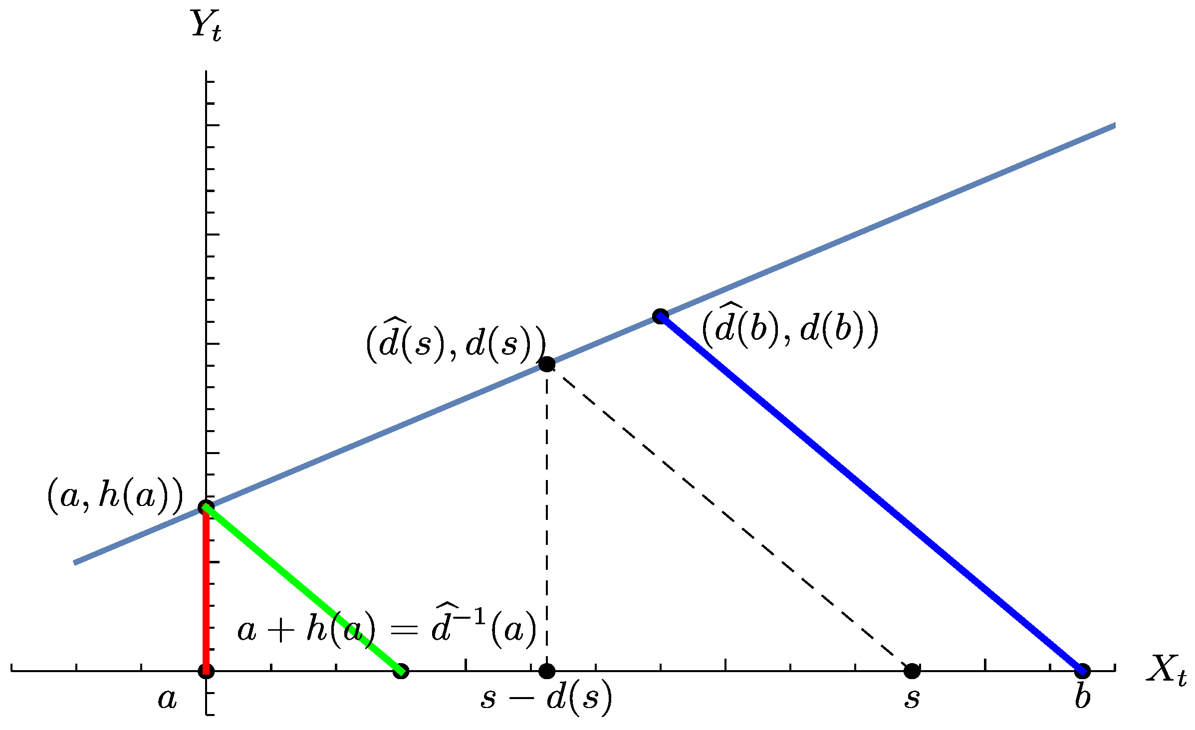
  • In the remaining case x a + d b , both drawdown and classic exits are possible. For the latter case, see Figure 1. The key observation here is that drawdown [classic] exits occur iff X t does [does not] cross the line x 1 = d + a . The final answers will combine these two cases.

3. The Three Laplace Transforms of the Exit Time out of a Rectangle for Lévy Processes without Positive Jumps

In this section we provide Laplace transforms of T R and of the eventual overshoot at T R . One can break down the analysis of T R to nine cases, depending on which of the three exit boundaries T a , , T b , + or τ d occurred, and on the three relations between x, a, b and d described above.
The following results are immediate applications of the strong Markov property and of known first passage and draw-down results.
Theorem 1.
Consider a spectrally negative Lévy process X with differentiable scale function W q . Then, for fixed d 0 and a x b , letting U b D , D b U denote the functions defined in (13), (15), we have:
a + d x b x a + d b b a + d I E x e q T b , + ; T b , + min ( τ d , T a , ) = U b D q , d b ( x ) Ψ ¯ q ( a + d ) ( x , a ) U b D q , d b ( a + d ) Ψ ¯ q b ( x , a ) I E x e q T a , + θ ( X T a , a ) ; T a , min ( τ d , T b , + ) = 0 Ψ q , θ ( a + d ) ( x , a ) Ψ q , θ b ( x , a ) I E x e q τ d θ ( Y τ d d ) ; τ d min ( T b , + , T a , ) = D b U q , θ , d b ( x ) Ψ ¯ q ( a + d ) ( x , a ) D b U q , θ , d b ( a + d ) 0
Proof. 
Please note that in the third column the d boundary is invisible and does not appear in the results, and in the first column the a boundary is invisible and does not appear in the results. These two cases follow therefore by applying already known results.
The middle column holds by breaking the path at the first crossing of a + d . The main points here are that
  • the middle case may happen only if X t visits a before a + d ;
  • the first case (exit through b) and the third case (drawdown exit) may happen only if X t visits first a + d , with the drawdown barrier being invisible, and that subsequently the lower first passage barrier a becomes invisible.
The results follow then due to the smooth crossing upward and the strong Markov property. □
Proof. 
Let us check the first and third row of the second column. Applying the strong Markov property at T a + d , + yields
I E x e q T b , + ; T b , + min ( τ d , T a , ) = I E x e q T b , + ; T a + d , + T a , I E a + d e q T b , + ; T b , + τ d = W q ( x a ) W q ( d ) e ( b a d ) W q ( d ) W q ( d )
and
I E x e q τ d θ ( Y τ d d ) ; τ d min ( T b , + , T a , ) = I E x e q τ d θ ( Y τ d d ) ; T a + d , + T a , I E a + d e q τ d θ ( Y τ d d ) ; τ d T b , + = W q ( x a ) W q ( d ) δ q , θ ( d ) 1 e ( b a d ) ) W q ( d ) W q ( d ) .
 □

4. Generalized Draw-Down Stopping for Processes without Positive Jumps

Generalized drawdown times appear naturally in the Azema Yor solution of the Skorokhod embedding problem Azéma and Yor (1979), and in the Dubbins-Shepp-Shiryaev, and Peskir-Hobson-Egami optimal stopping problems Dubins et al. (1994); Egami and Oryu (2015); Hobson (2007); Peskir (1998). Importantly, they allow a unified treatment of classic first passage and drawdown times (see also Avram et al. (2018b) for a further generalization to taxed processes)—see Avram et al. (2017b); Li et al. (2017). The idea is to replace the upper side of the rectangle R by a parametrized curve
( x 1 , x 2 ) = ( d ^ ( s ) , d ( s ) ) , d ^ ( s ) = s d ( s ) ,
where s = x 1 + x 2 represents the value of X ¯ t during the excursion which intersects the upper boundary at ( x 1 , x 2 ) (see Figure 2). Alternatively, parametrizing by x yields
y = h ( x ) , h ( x ) = d ^ 1 ( x ) x .
Definition 1.
Li et al. (2017) For any function d ( s ) > 0 such that d ^ ( s ) = s d ( s ) is nondecreasing, a generalized drawdown time is defined by
τ d ^ ( · ) : = inf { t 0 : Y t > d ( X ¯ t ) } = inf t 0 : X t < d ^ ( X ¯ t ) .
Such times provide a natural unification of classic and drawdown times.
Introduce
Y ˜ t : = Y t d ( X ¯ t ) , t 0
to be called draw-down type process. Please note that we have Y ˜ 0 = d ^ ( X 0 ) < 0 , and that the process Y ˜ t is in general non-Markovian. However, it is Markovian during each negative excursion of X t , along one of the oblique lines in the geometric decomposition sketched in Figure 1.
Example 1.
With affine functions
d ( s ) = ( 1 ξ ) s + d d ^ ( s ) = ξ s d , ξ [ 0 , 1 ] , d > 0 ,
we obtain the affine draw-down/regret times studied in Avram et al. (2017b).
Affine drawdown times reduce to a classic drawdown time (3) when ξ = 1 , d ( s ) = d , and to a ruin time when ξ = 0 , d ^ ( s ) = d , d ( s ) = s + d . When ξ varies, we are dealing with the pencil of lines passing through ( x 1 , x 2 ) = ( d , d ) . In particular, for ξ = 1 we obtain the rectangle case from Section 3, and for ξ = 0 we have an infinite strip with a vertical boundary at x 1 = d .
One of the merits of affine drawdown times is that they allow unifying the classic first passage theory with the drawdown theory Avram et al. (2017b); in particular, the generalized drawdown functions (23) below unify the classic and drawdown survival and ruin probabilities (and have relatively simple formulas as well—see Avram et al. (2017a)).
Introduce now generalized drawdown analogues of the drawdown survival and ruin probabilities (12) for which we will use the same notation:
U b D q , d ^ ( · ) b ( x ) = I E x e q T b , + ; T b , + τ d ^ ( · ) D b U q , θ , d ^ ( · ) b ( x ) ) = I E x e q τ d ^ ( · ) θ Y ˜ τ d ^ ( · ) ; τ d ^ ( · ) < T b + .
Remark 6.
In the spectrally negative case, these functions may be represented as integrals:
U b D q , d ^ ( · ) b ( x ) = e x b ν q ( s , d ^ ( s ) ) d s , D b U q , θ , d ^ ( · ) b ( x ) = x b e x y ν q ( s , d ^ ( s ) ) d s ν q ( y , d ^ ( y ) ) δ q , θ ( y , d ^ ( y ) ) d y ,
where ν q ( y , d ^ ( y ) ) , δ q , θ ( y , d ^ ( y ) ) are defined in (9), (10).
This is already apparent in (Landriault et al. 2017b, Cor 3.1), and may be easily understood probabilistically from Figure 2: the first equation is the probability of no occurrence in a non-homogeneous Poisson process, and the second decomposes the transform of the deficit, by conditioning on the point y [ x , b ] where the maximum occurred.
We provide now a heuristic proof valid for the Lévy case when ν q ( y , d ^ ( y ) ) = ν q ( y d ^ ( y ) ) = ν q ( d ( y ) ) and δ q , θ ( y , d ^ ( y ) ) = δ q , θ ( y d ^ ( y ) ) = δ q , θ ( d ( y ) ) .
1.
Due to creeping, U b D is a product of infinitesimal events
Ψ ¯ q y + ϵ ( y , y d ( y ) ) = W q ( d ( y ) ) W q ( d ( y ) + ϵ ) 1 ϵ ν q ( d ( y ) ) e ϵ ν q ( d ( y ) ) .
Taking product, with ϵ = d y , yields (24).
2.
Informally, we condition on the density X ¯ t d y . The integrand of D b U is obtained multiplying survival infinitesimal events up to level y by an infinitesimal termination event in [ y , y + d y ] . The probability of this event, conditioned on survival up to y, is given by the deficit formula
Ψ q , θ y + ϵ ( y , y d ( y ) ) = Z q , θ ( d ( y ) ) W q ( d ( y ) ) Z q , θ ( d ( y ) + ϵ ) W q ( d ( y ) + ϵ ) ϵ ( Z q , θ ( d ( y ) ) + ν q ( d ( y ) ) Z q , θ ( d ( y ) ) = ϵ ν q ( d ( y ) ) δ q , θ ( d ( y ) )
For a rigorous (rather intricate) proof, see Avram et al. (2018b).
The end result for generalized drawdown times is (Avram et al. 2018b, Thm1):
Theorem 2.
Consider a process X for which the functions Ψ , Ψ ¯ are differentiable in the upper variable b. Assume d ( x ) > 0 and d ^ ( x ) = x d ( x ) nondecreasing. Then, q , θ 0 , b R , the functions U b D ( x ) = U b D q b ( x , d ^ ( · ) ) , D b U ( x ) = D b U q , θ b ( x , d ^ ( · ) ) satisfy (24). Alternatively, they satisfy the ODE’s
U b D ( y ) ν q ( y , d ^ ( y ) ) U b D ( y ) = 0 , U b D ( b ) = 1 ,
D b U ( y ) ν q ( y , d ^ ( y ) ) D b U ( y ) + δ q , θ ( y , d ^ ( y ) ) = 0 , D b U ( b ) = 0 .
Remark 7.
The operator involved in the ODE’s above is the generator of the upward ladder process, under time and spatial killing, and with the downward excursions excised. Once this known, variations involving different boundary conditions are easily obtained as well.

5. The Three Laplace Transforms of the Exit Time out of a Curved Trapezoid, for Processes without Positive Jumps

We will replace now the classic drawdown time in Section 3 by a generalized one. Similar geometric considerations, with d ( · ) , a + h ( a ) replacing d , a + d in Theorem 1, yield:
Theorem 3.
Consider a spectrally negative Lévy process X with differentiable scale function W q . Then, for a x b and d ( · ) satisfying the conditions of Definition 1, we have:
a + h ( a ) x x a + h ( a ) b b a + h ( a ) I E x e q T b , + ; T b , + min ( τ d ^ ( · ) , T a , ) = U b D q , d ^ ( · ) b ( x ) Ψ ¯ q a + h ( a ) ( x , a ) U b D q , d ^ ( · ) b ( a + h ( a ) ) Ψ ¯ q b ( x , a ) I E x e q T a , + θ ( X T a , a ) ; T a , min ( τ d ^ ( · ) , T b , + ) = 0 Ψ q , θ a + h ( a ) ( x , a ) Ψ q , θ b ( x , a ) I E x e q τ d ^ ( · ) θ ( Y τ d ^ ( · ) d ) ; τ d ^ ( · ) min ( T b , + , T a , ) = D b U q , θ , d ^ ( · ) b ( x ) Ψ ¯ q a + h ( a ) ( x , a ) D b U q , θ , d ^ ( · ) b ( a + h ( a ) ) 0
Proof. 
Note that if b a + h ( a ) (narrow band), it is again impossible for the process to leave R through the upper boundary of R , and T R reduces to T a , T b , + , and nothing changes. Similarly, if a + h ( a ) x (flat band), it is impossible for the process to leave R through the left boundary of R , and T R reduces to T b , + τ d . Finally, the two zones in the intermediate case are separated by a + h ( a ) (instead of a + d ). □

6. de Finetti’s Optimal Dividends for Spectrally Negative Markov Processes with Generalized Draw-Down Stopping

In this section, we revisit the de Finetti’s optimal dividend problem for spectrally negative Markov processes with the point b becoming a reflecting boundary, instead of absorbing, as it was in Section 3.
Define the Skorokhod reflected/constrained process at first passage times below or above by:
X t [ a = X t + L t , X t b ] = X t U t .
Here
L t = L t [ a = ( X ̲ t a ) , U t = U t b ] = X ¯ t b +
are the minimal “Skorohod regulators” constraining X t to be bigger than a, and smaller than b, respectively.
Let now
V b ] ( x ) = V q , d ^ ( · ) b ] ( x ) : = I E x 0 τ d ^ ( · ) T a , e q t d U t b ]
denote the present value of all dividend payments at b, until the first passage time either below a, or below the drawdown boundary for the process X t b ] reflected at b, starting from x b (a generalization of the famous de Finetti objective). By the strong Markov property, it holds that
V b ] ( x ) = I E x e q T b , + ; T b , + min ( τ d ^ ( · ) , T a , ) v ( b ) , v ( b ) = v q ( b , d ^ ( b ) ) : = I E b 0 τ d ^ ( · ) e q t d U t b ] .
Remark 8.
The function v ( b ) , the expected discounted time until killing for the reflected process, when starting from b, equals the time the process reflected at b spends at point ( b , 0 ) in Figure 2, before a downward excursion beyond d ^ ( b ) kills the process. In the Lévy case, it is well-known Kyprianou (2014) that this time is exponential with parameter ν q ( b , d ^ ( b ) ) , and thus its expectation is the reciprocal of the killing parameter ν q ( b , d ^ ( b ) ) , i.e.,
v ( b ) = ν q ( b , d ^ ( b ) ) 1
Excursion theoretic arguments show that (31) continues to hold in the spectrally negative Markov case (for a proof under a similar setup, see (Czarna et al. 2018, sct. 4)).
Furthermore, by (Avram et al. 2018b, Thm. 1) included above as (24), it holds that
I E x e q T b , + 1 T b , + < τ d ( · ) = e x b ν q ( z , d ^ ( z ) ) d z .
When a = , we arrive finally to an explicit formula
V b ] ( x ) = e x b ν q ( y , d ^ ( y ) ) d s ν q ( b , d ^ ( b ) )
expressing the expected dividends in terms of ν q ( y , d ^ ( y ) ) . Please note that in the Lévy case Equation (33) simplifies to:
V b ] ( x ) = W q ( d ( x ) ) W q ( d ( b ) ) ν q ( d ( b ) ) 1
(using x l ( x ) = d ( x ) ), which checks with (Wang and Zhou 2018, Lem. 3.1–3.2).
The problem of choosing a drawdown boundary to optimize dividends in (33) is solved in Avram and Goreac (2018) via Pontryaghin’s maximum principle.

7. Example: Affine Draw-Down Stopping for Brownian Motion

Consider optimizing expected dividends V b ] ( x ) given in Equation (29) with respect to the optimal dividend barrier b for Brownian motion with drift X ( t ) = σ B t + μ t and with affine drawdown stopping d ( x ) = ( 1 ξ ) x + d , where ξ [ 0 , 1 ] , d 0 , a x b .
Please note that if a + h ( a ) > b , where h ( x ) = d ( x ) / ξ , then the drawdown constraint is invisible, and the problem reduces to the classical de Finetti objective. Hence, we consider a + h ( a ) b .
The scale function of Brownian motion is
W q ( x ) = 2 e μ x / σ 2 Δ sinh ( x Δ / σ 2 ) = 1 Δ [ e ( μ + Δ ) x / σ 2 e ( μ + Δ ) x / σ 2 ] ,
where Δ = μ 2 + 2 q σ 2 . Assume that x a + h ( a ) = a + d ( a ) ξ = a + d ξ , then as a special case of spectrally negative Levy process, the expected dividends for Brownian motion equals
V b ] ( x ) = I E x e q T b , + ; T b , + min ( τ d ^ ( · ) , T a , ) v ( b ) = W q ( d ( x ) ) W q ( d ( b ) ) 1 1 ξ W q ( d ( b ) ) W q ( d ( b ) ) ,
see (Avram et al. 2017b, Thm. 1.1), with tax parameter γ = 0 , and (Avram et al. 2017b, Rem. 7), with tax parameter γ = 1 . The barrier influence function which must be optimized in b becomes
B I ( b , d , ξ ) = W q ( ( 1 ξ ) x + d ) 1 1 1 ξ W q ( ( 1 ξ ) x + d ) = σ 2 2 e x μ / σ 2 csch x μ 2 + 2 q σ 2 / σ 2 coth ( d + x x ξ ) μ 2 + 2 q σ 2 / σ 2 μ / μ 2 + 2 q σ 2 .
The critical point b satisfies
W q W q ( W q ) 2 ( ( 1 ξ ) b + d ) = ξ 1 ξ ,
that is b satisfies
q σ 2 + μ 2 + μ 2 q σ 2 + μ 2 sinh 2 b 2 q σ 2 + μ 2 σ 2 q σ 2 + μ 2 cosh 2 b 2 q σ 2 + μ 2 σ 2 2 q σ 2 + μ 2 cosh b 2 q σ 2 + μ 2 σ 2 μ sinh b 2 q σ 2 + μ 2 σ 2 2 = ξ 1 ξ .
In Figure 3 given below, we have an illustration of plot of barrier influence function and its derivative for Brownian motion with drift μ = 1 / 2 and σ = 1 .
Remark 9.
Please note that once ξ is fixed, we get nontrivial results for the optimal barrier. However, if we maximize over ξ as well, the optimum is achieved by the classical de Finetti solution ξ = 0 W q ( b + d ) = 0 , corresponding to forced stopping below d (d is just a shift of the origin, with respect to the classical solution W q ( b ) = 0 ) Avram and Goreac (2018). In the diffusion case, it is not yet known whether examples in which the generalized de Finetti problem improves on the classic de Finetti solution are possible.
Remark 10.
Let us note now that Equation (36) holds in fact for any spectrally negative Lévy process. Similar computations may be therefore performed for any spectrally negative Levy process, by plugging exact or approximate formulas for the scale function into the function
W q W q ( W q ) 2
which is required to solve (36).
The easiest case is the Cramér-Lundberg process with phase-type claims, since in this case the scale function is a sum of exponentials. For example, for a Cramér-Lundberg process with premium rate c > 0 , Poisson arrivals of intensity λ and exponential claims with mean 1 / μ , the scale function is W q ( x ) = c 1 ( μ + Δ + Δ + Δ e Δ + x μ + Δ Δ + Δ e Δ x ) , x 0 , where Δ ± = q + λ μ c ± ( q + λ μ c ) 2 + 4 c q μ 2 c , and similar computations may be performed (see also (Wang and Zhou 2018, Example 5.2)).

Author Contributions

Conceptualization, F.A.; Formal analysis, F.A. and C.V.-A.; Project administration, F.A.; Supervision, F.A.; Validation, D.G., C.V.-A.; Writing—original draft, F.A. and C.V.-A.; Writing—review, editing, D.G., C.V.-A.

Funding

This work is supported by the Scientific and Technological Research Council of Turkey, TUBITAK Project No. 117F273.

Acknowledgments

We thank Ali Devin Sezer for useful discussions.

Conflicts of Interest

The authors declare no conflict of interest.

References

  1. Albrecher, Hansjörg, and Sören Asmussen. 2010. Ruin Probabilities. Singapore: World Scientific, vol. 14. [Google Scholar]
  2. Albrecher, Hansjörg, Florin Avram, Corina Constantinescu, and Jevgenijs Ivanovs. 2014. The tax identity for Markov additive risk processes. Methodology and Computing in Applied Probability 16: 245–58. [Google Scholar] [CrossRef]
  3. Albrecher, Hansjörg, Jevgenijs Ivanovs, and Xiaowen Zhou. 2016. Exit identities for Lévy processes observed at Poisson arrival times. Bernoulli 22: 1364–82. [Google Scholar] [CrossRef]
  4. Avram, Florin, and J. P. Garmendia. 2019. Some first passage theory for the Segerdahl-Tichy risk process, and open problems. Forthcoming. [Google Scholar]
  5. Avram, Florin, and Dan Goreac. 2018. A pontryaghin maximum principle approach for the optimization of dividends/consumption of spectrally negative Markov processes, until a generalized draw-down time. arXiv, arXiv:1812.08438. [Google Scholar]
  6. Avram, Florin, Andreas E. Kyprianou, and Martijn R. Pistorius. 2004. Exit problems for spectrally negative Lévy processes and applications to (Canadized) Russian options. The Annals of Applied Probability 14: 215–38. [Google Scholar]
  7. Avram, Florin, Zbigniew Palmowski, and Martijn R. Pistorius. 2007. On the optimal dividend problem for a spectrally negative Lévy process. The Annals of Applied Probability 17: 156–80. [Google Scholar] [CrossRef]
  8. Avram, Florin, Zbigniew Palmowski, and Martijn R. Pistorius. 2015. On Gerber–Shiu functions and optimal dividend distribution for a Lévy risk process in the presence of a penalty function. The Annals of Applied Probability 25: 1868–935. [Google Scholar] [CrossRef]
  9. Avram, Florin, Danijel Grahovac, and Ceren Vardar-Acar. 2017a. The W,Z scale functions kit for first passage problems of spectrally negative Lévy processes, and applications to the optimization of dividends. arXiv, arXiv:1706.06841. [Google Scholar]
  10. Avram, Florin, Nhat Linh Vu, and Xiaowen Zhou. 2017b. On taxed spectrally negative Lévy processes with draw-down stopping. Insurance: Mathematics and Economics 76: 69–74. [Google Scholar] [CrossRef]
  11. Avram, Florin, José-Luis Pérez, and Kazutoshi Yamazaki. 2018a. Spectrally negative Lévy processes with Parisian reflection below and classical reflection above. Stochastic Processes and Their Applications 128: 255–90. [Google Scholar] [CrossRef]
  12. Avram, Florin, Bin Li, and Shu Li. 2018b. A unified analysis of taxed draw-down spectrally negative Markov processes. Forthcoming. [Google Scholar]
  13. Avram, Florin, and Matija Vidmar. 2017. First passage problems for upwards skip-free random walks via the Φ,W,Z paradigm. arXiv, arXiv:1708.06080. [Google Scholar]
  14. Avram, Florin, and Xiaowen Zhou. 2017. On fluctuation theory for spectrally negative Lévy processes with parisian reflection below, and applications. Theory of Probability and Mathematical Statistics 95: 17–40. [Google Scholar] [CrossRef]
  15. Azéma, Jacques, and Marc Yor. 1979. Une solution simple au probleme de Skorokhod. In Séminaire de Probabilités XIII. Berlin: Springer, pp. 90–115. [Google Scholar]
  16. Bertoin, Jean. 1997. Exponential decay and ergodicity of completely asymmetric Lévy processes in a finite interval. The Annals of Applied Probability 7: 156–69. [Google Scholar] [CrossRef]
  17. Bertoin, Jean. 1998. Lévy Processes. Cambridge: Cambridge University Press, vol.121. [Google Scholar]
  18. Borovkov, Alexandr. 2012. Stochastic Processes in Queueing Theory. Berlin: Springer Science & Business Media, vol. 4. [Google Scholar]
  19. Carr, Peter. 2014. First-order calculus and option pricing. Journal of Financial Engineering 1: 1450009. [Google Scholar] [CrossRef]
  20. Chan, Terence, Andreas E. Kyprianou, and Mladen Savov. 2011. Smoothness of scale functions for spectrally negative Lévy processes. Probability Theory and Related Fields 150: 691–708. [Google Scholar] [CrossRef]
  21. Czarna, Irmina, José-Luis Pérez, Tomasz Rolski, and Kazutoshi Yamazaki. 2017. Fluctuation theory for level-dependent Lévy risk processes. arXiv, arXiv:1712.00050. [Google Scholar]
  22. Czarna, Irmina, Adam Kaszubowski, Shu Li, and Zbigniew Palmowski. 2018. Fluctuation identities for omega-killed Markov additive processes and dividend problem. arXiv, arXiv:1806.08102. [Google Scholar]
  23. Dubins, Lester E., Larry A. Shepp, and Albert Nikolaevich Shiryaev. 1994. Optimal stopping rules and maximal inequalities for Bessel processes. Theory of Probability & Its Applications 38: 226–61. [Google Scholar]
  24. Egami, Masahiko, and Tadao Oryu. 2015. An excursion-theoretic approach to regulator’s bank reorganization problem. Operations Research 63: 527–39. [Google Scholar] [CrossRef]
  25. Hobson, David. 2007. Optimal stopping of the maximum process: A converse to the results of Peskir. Stochastics An International Journal of Probability and Stochastic Processes 79: 85–102. [Google Scholar] [CrossRef]
  26. Ivanovs, Jevgenijs, and Zbigniew Palmowski. 2012. Occupation densities in solving exit problems for Markov additive processes and their reflections. Stochastic Processes and Their Applications 122: 3342–60. [Google Scholar] [CrossRef]
  27. Jacobsen, Martin, and Anders Tolver Jensen. 2007. Exit times for a class of piecewise exponential Markov processes with two-sided jumps. Stochastic Processes and Their Applications 117: 1330–56. [Google Scholar] [CrossRef]
  28. Kyprianou, Andreas. 2014. Fluctuations of Lévy Processes with Applications: Introductory Lectures. Berlin: Springer Science & Business Media. [Google Scholar]
  29. Landriault, David, Bin Li, and Shu Li. 2015. Analysis of a drawdown-based regime-switching Lévy insurance model. Insurance: Mathematics and Economics 60: 98–107. [Google Scholar] [CrossRef]
  30. Landriault, David, Bin Li, and Hongzhong Zhang. 2017a. On magnitude, asymptotics and duration of drawdowns for Lévy models. Bernoulli 23: 432–58. [Google Scholar] [CrossRef]
  31. Landriault, David, Bin Li, and Hongzhong Zhang. 2017b. A unified approach for drawdown (drawup) of time-homogeneous Markov processes. Journal of Applied Probability 54: 603–26. [Google Scholar] [CrossRef]
  32. Lehoczky, John P. 1977. Formulas for stopped diffusion processes with stopping times based on the maximum. The Annals of Probability 5: 601–7. [Google Scholar] [CrossRef]
  33. Li, Bo, Linh Vu, and Xiaowen Zhou. 2017. Exit problems for general draw-down times of spectrally negative Lévy processes. arXiv, arXiv:1702.07259. [Google Scholar]
  34. Li, Bo, and Xiaowen Zhou. 2018. On weighted occupation times for refracted spectrally negative Lévy processes. Journal of Mathematical Analysis and Applications 466: 215–37. [Google Scholar] [CrossRef]
  35. Mijatovic, Aleksandar, and Martijn R Pistorius. 2012. On the drawdown of completely asymmetric Lévy processes. Stochastic Processes and Their Applications 122: 3812–36. [Google Scholar] [CrossRef]
  36. Page, Ewan S. 1954. Continuous inspection schemes. Biometrika 41: 100–15. [Google Scholar] [CrossRef]
  37. Peskir, Goran. 1998. Optimal stopping of the maximum process: The maximality principle. Annals of Probability 26: 1614–40. [Google Scholar] [CrossRef]
  38. Pistorius, Martijn R. 2004. On exit and ergodicity of the spectrally one-sided Lévy process reflected at its infimum. Journal of Theoretical Probability 17: 183–220. [Google Scholar] [CrossRef]
  39. Shepp, Larry, and Albert N. Shiryaev. 1993. The Russian option: Reduced regret. The Annals of Applied Probability 3: 631–40. [Google Scholar] [CrossRef]
  40. Suprun, V. N. 1976. Problem of destruction and resolvent of a terminating process with independent increments. Ukrainian Mathematical Journal 28: 39–51. [Google Scholar] [CrossRef]
  41. Taylor, Howard M. 1975. A stopped Brownian motion formula. The Annals of Probability 3: 234–46. [Google Scholar] [CrossRef]
  42. Wang, Wenyuan, and Xiaowen Zhou. 2018. General drawdown-based de Finetti optimization for spectrally negative Lévy risk processes. Journal of Applied Probability 55: 513–42. [Google Scholar] [CrossRef]
1
The fact that the survival probability has the multiplicative structure (2) is equivalent to the absence of positive jumps, by the strong Markov property.
2
Please note that (Mijatovic and Pistorius 2012, Thm. 1) give a more complicated “sextuple law” with two cases, and that (Landriault et al. 2017a, Thm 3.1) use an alternative to the function Z q ( x , θ ) , so that some computing is required to get (11) and (14).
3
Choosing a , b , d optimally in various control problems involving optimal dividends and capital injections should be of interest, and will be pursued in further work.
Figure 1. A sample path of ( X , Y ) with X a spectrally negative Lévy process. The region R has d = 10 , a = 6 and b = 7 ; the dark boundary shows the possible exit points of ( X , Y ) from R. The base of the red line separates R in two parts with different behavior.
Risks 07 00018 g001
Figure 2. Affine drawdown exit of ( X , Y ) d ( s ) = 1 3 s + 1 .
Risks 07 00018 g002
Figure 3. Optimizing dividends with affine drawdown stopping where μ = 1 / 2 , q = 1 / 10 , σ = 1 , ξ = 1 / 3 , b = 20 , d = 1 . The critical point b = 2.12445 .
Risks 07 00018 g003

