Phase-Type Models in Life Insurance: Fitting and Valuation of Equity-Linked Benefits

Abstract

Phase-type (PH) distributions are defined as distributions of lifetimes of finite continuous-time Markov processes. Their traditional applications are in queueing, insurance risk, and reliability, but more recently, also in finance and, though to a lesser extent, to life and health insurance. The advantage is that PH distributions form a dense class and that problems having explicit solutions for exponential distributions typically become computationally tractable under PH assumptions. In the first part of this paper, fitting of PH distributions to human lifetimes is considered. The class of generalized Coxian distributions is given special attention. In part, some new software is developed. In the second part, pricing of life insurance products such as guaranteed minimum death benefit and high-water benefit is treated for the case where the lifetime distribution is approximated by a PH distribution and the underlying asset price process is described by a jump diffusion with PH jumps. The expressions are typically explicit in terms of matrix-exponentials involving two matrices closely related to the Wiener-Hopf factorization, for which recently, a Lévy process version has been developed for a PH horizon. The computational power of the method of the approach is illustrated via a number of numerical examples.

1. Introduction

A random variable (r.v.) $\tau$ is phase-type (PH) with representation $(\mathit{\alpha },\mathit{T})$ if it is distributed as the lifetime $inf\{t\ge 0:J_t=†\}$ of a killed (terminating) time-homogenous Markov process $J=$${\left\{J_t\right\}}_{t\ge 0}$ with $p<\infty$ states, initial distribution $\mathit{\alpha }$ (a row vector), and generator $\mathit{T}$, where † is an additional absorbing state. PH distributions originate from queueing theory and the work of A.K. Erlang, A. Jensen and M.F. Neuts. However, in recent decades, they have found numerous applications to different areas. The main reason for this is that many calculations that are explicit for exponential distributions are often computationally tractable with PH assumptions and that, in addition, PH distributions are dense so that a given distribution F on $[0,\infty )$ can be approximated arbitrarily well by a PH distribution provided one takes p large enough. For surveys of the theory and applications, see (Asmussen 2003; Asmussen and Albrecher 2010; Bladt and Nielsen 2017). The present paper is concerned with some applications to life insurance, an area where PH distributions have been far less employed than in the related areas of non-life insurance. There are many papers in ruin theory that assume that claim sizes are PH distributed; see (Cai and Li 2005b) and the review paper (Bladt 2005). Some papers assume that the claim time is PH distributed; see (Stanford et al. 2000). (Zadeh et al. 2014) considered disability insurance using a PH model. (Zadeh and Stanford 2016) studied credibility theory using PH distributions. In finance, PH distributions have also been used extensively. For example, (Asmussen et al. 2004) considered option pricing under an exponential phase-type Lévy model; (Cai and Li 2005a) dealt with applications of PH distributions to risk measures; and (Egami and Yamazaki 2014) considered PH approximations of Lévy models. On the contrary, the only references of applications of PH distributions to life insurance we know of are (Lin and Liu 2007) and (Zadeh et al. 2014).

The motivation for the present study is some valuation problems of equity-linked products in life insurance considered in Gerber et al. (2012, 2013, 2015) (GSY). Let $\tau ={\tau }_x$ be the remaining lifetime of an insured of age x when signing the contract, then the payment of this class of benefits has the form $\mathrm{\Psi }({\overline{S}}_{\tau },S_{\tau })$ where $S_t$ is the price at time t of some stock or stock index and ${\overline{S}}_t={max}_{v\le t}{S}_t$ the running maximum. An example of such a benefit is the guaranteed minimum death benefit (GMDB) $max(S_{\tau },K)$, but there are many others; see the list in Section 4. Defining $X_t$ as $X_t=log(S_t/S_0)$, $M_t={\overline{X}}_t$ as the running maximum of X, and $D_t=M_t-X_t$ as the displacement from the maximum, we then have:

$$\mathrm{\Psi }({\overline{S}}_{\tau },S_{\tau })=\mathrm{\Phi }(M_{\tau },D_{\tau })\mathrm{where}\mathrm{\Phi }(m,d)=\mathrm{\Psi }(S_0{\mathrm{e}}^m,S_0{\mathrm{e}}^{m-d)})$$

(1)

(note that $X_t=M_t-D_t$), and the fair value of the benefit is the expected discounted payment.

A widely-used model (Cont and Tankov 2004) assumes that $X=$${\left\{X_t\right\}}_{t\ge 0}$ is a Lévy process, and the key vehicle in GSY for the computations for such expectations is the classical Wiener-Hopf factorization:

Lemma 1.

For a Lévy process $X_t$ and an independent exponential time τ, the r.v.’s $M_{\tau }={max}_{0\le s\le \tau }{X}_s$ and $D_{\tau }=M_{\tau }-X_{\tau }$ are independent. Further,

$$D_{\tau }\stackrel{\mathrm{d}}{=}-{\underline{X}}_{\tau }=-\underset{0\le s\le \tau }{min}{X}_s.$$

For the geometric Brownian motion model where X is a Brownian motion (BM) with drift, $M_{\tau }$ and $D_{\tau }$ both have an exponential distribution, and for more general jump diffusions, a number of computational procedures have been developed (see Section 5 for references). In GSY, they approximate the density/tail of ${\tau }_x$ by a linear combination of exponential terms, which allows them to reduce the computations to simple integrations using Lemma 1.

The approximation of the distribution of ${\tau }_x$ by a linear combination of exponential terms in GSY uses an ad hoc optimization procedure. The main problem there is that it is very difficult to make the linear combination of exponential densities to be a density function; in particular, very often, in the tail part, the linear combination of exponential densities can be negative. Since, in the application to valuing equity-linked insurance products, the distribution at the tail part plays an important role, this motivated us to consider using the PH distribution to approximate the future lifetime distribution. For PH distributions, more classical statistical methods using maximum likelihood have, however, been developed (Asmussen et al. 1996), and in view of the denseness of PH distributions and the fact that they have proven a computationally-tractable generalization of the exponential distribution in other settings, a natural idea is therefore to use a PH approximation $\tau$ to ${\tau }_x$. The first step in implementing this for pricing equity-linked benefits is to develop a version of the Wiener-Hopf factorization for the case where $\tau$ is PH and independent of X. This has been done in a companion paper (Asmussen and Ivanovs 2019), and the contribution of the present paper is to provide the further steps such as PH fitting of human mortality and computations of prices of equity-linked benefits for BM and jump diffusions.

2. Preliminaries

The vector of killing rates of a PH$(\mathit{\alpha },\mathit{T})$ r.v. $\tau$ is given by $\mathit{t}=-\mathit{T}\mathbf{1}$, where $\mathbf{1}$ is a column vector with all entries equal to one. The density is $\mathit{\alpha }{\mathrm{e}}^{\mathit{T}z}\mathit{t}$, and the tail $\mathbb{P}(\tau >z)$ is $\mathit{\alpha }{\mathrm{e}}^{\mathit{T}z}\mathbf{1}$. Here, the exponential ${\mathrm{e}}^{\mathit{R}}$ of a matrix is defined as ${\sum }_0^{\infty }{\mathit{R}}^n/n!$. We shall often use formulas like:

$${\int }_a^b{\mathrm{e}}^{\mathit{R}x}\mathrm{d}x={\mathit{R}}^{-1}({\mathrm{e}}^{\mathit{R}b}-{\mathrm{e}}^{\mathit{R}a})=({\mathrm{e}}^{\mathit{R}b}-{\mathrm{e}}^{\mathit{R}a}){\mathit{R}}^{-1},{\int }_0^{\infty }{\mathrm{e}}^{\mathit{R}x}\mathrm{d}x=-{\mathit{R}}^{-1},$$

that are immediate analogues of standard formulas for univariate exponentials. For example, taking $\mathit{R}=-s\mathit{I}+\mathit{T}$ gives the Laplace transform $\mathbb{E}\left[{\mathrm{e}}^{-s\tau }\right]$ as $\mathit{\alpha }{(s\mathit{I}-\mathit{T})}^{-1}\mathit{t}$. Of course, the existence of ${\mathit{R}}^{-1}$ has to be verified, which for a PH generator $\mathit{R}=\mathit{T}$ is a standard fact.

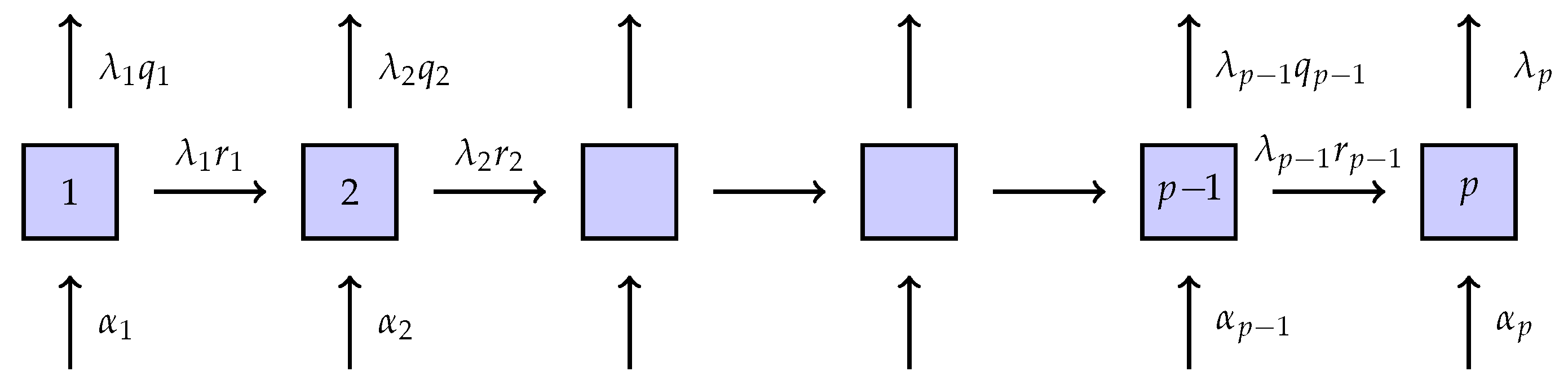
The subclass of generalized Coxian (GC) distributions will play a particular role. Here, the states are run through in lexicographical order, with exponential $\left({\lambda }_i\right)$ holding time in state i, and it is possible to enter or exit from any state (see Figure 1), where $q_i$ is the probability of exit after a visit to i and $r_i=1-q_i$ the probability of going to the next state. The structure of Coxian distributions is similar, except that only State 1 can be entered so that ${\alpha }_1=1$. Coxian distributions are in particular used in (Lin and Liu 2007) and (Zadeh et al. 2014).

Figure 1. A GC distribution.

Remark 1.

Though computational tractability and denseness are the main reasons for the popularity of PH distributions, other advantages have also sometimes been advocated. For example, whereas in the majority of examples, the PH modeling is purely descriptive, there are others where attempts have been made to give the Markov states a physical meaning like in compartment models and, in the life insurance context, in (Lin and Liu 2007) and (Zadeh et al. 2014). This makes the number p of phases quite large there, of order 200, whereas we have taken the descriptive point of view. The fit obviously becomes better when increasing p, but how good it needs to be depends very much on what it will be used for. In this paper, we consider the valuation problem, that is to calculate the net premium (expected discounted payoff) for equity-linked insurance products, and our numerical examples will show that taking $p=50$ will be sufficient for the precision one needs in this context.

3. PH Fits of Human Mortality Data

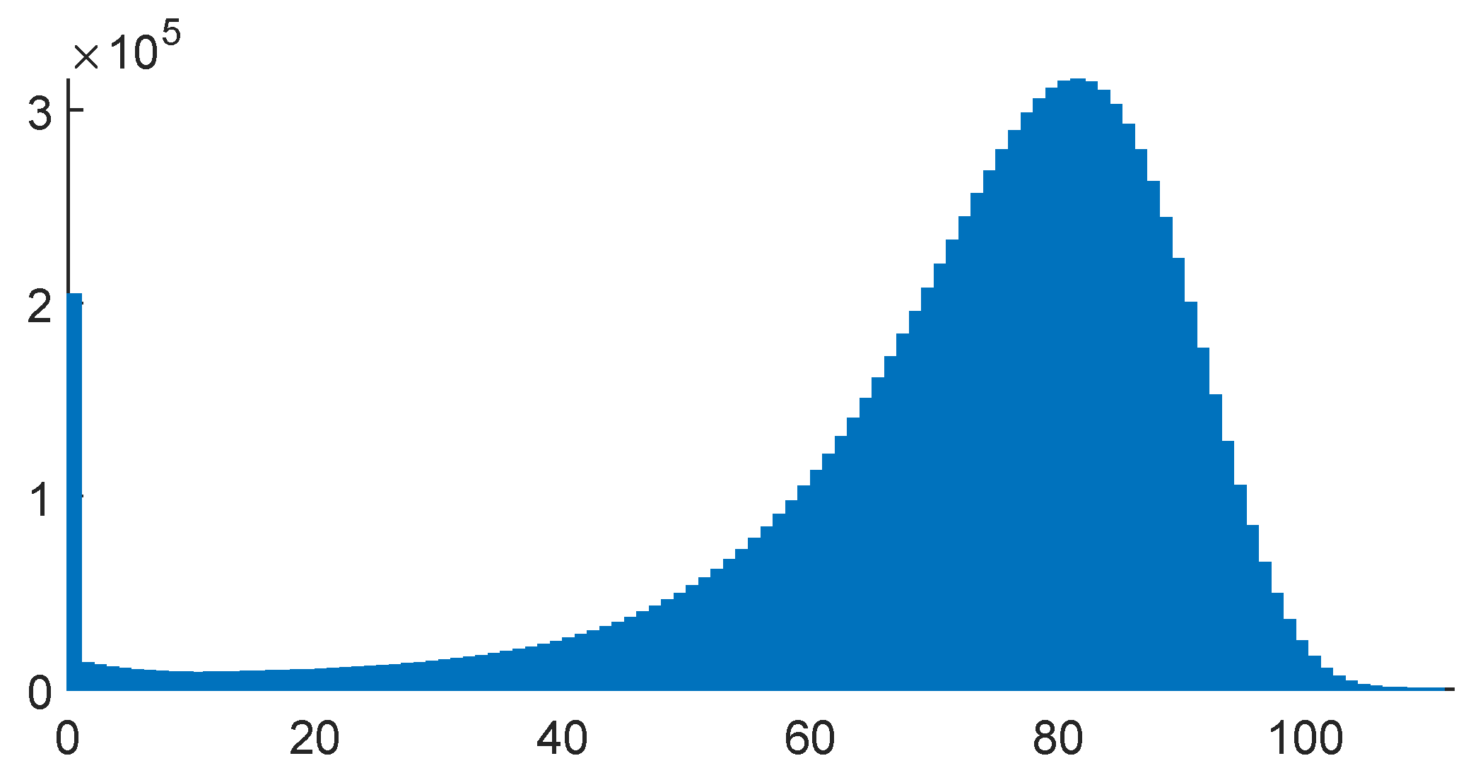
The distribution of human lifetimes of course varies somewhat according to the period where the data were collected, geographical and social conditions, etc., but the basic shapes are much alike. We have therefore concentrated on a single example, the illustrative life table in Appendix 2A of (Bowers et al. 1997). The form of the distribution, as illustrated via the number of deaths in consecutive years, is given in Figure 2.

Figure 2. Life table data.

We use an EM algorithm to fit various types of phase-type distributions to this life table. This idea was originally developed in (Asmussen et al. 1996), with the case of censored data and other implementation details given in (Olsson 1996). Olsson (Olsson 1998) has written a C implementation of this algorithm called EMpht, which is available online. The overwhelming computational burden is in the E step, where many complicated integrals involving matrix exponentials must be evaluated. This is done approximately by converting the problem into a system of ODEs, which are approximately solved via a Runge-Kutta method. While the original C implementation is still very adequate for creating fits with a small number of phases p, it can be improved upon for larger p.

We wrote a new implementation using the Julia language. It allows for the E step to be evaluated in three different ways: (i) using an ODE solver (as in (Asmussen et al. 1996; Olsson 1996)), (ii) using quadrature methods, and (iii) using the uniformization method of Okamura et al. Okamura et al. (2011a, 2011b). We used this last method to generate the fits found later in this paper; the code we used to create the figures below will be made available online (Asmussen et al. 2019). Each fit was given one hour execution time restricted to one thread on the processor Intel(R) Xeon(R) CPU E5-2698 v4 @ 2.20 GHz. The EM algorithm could have been terminated much earlier without a major difference to the quality of the fits, but as we were comparing the various values of p, we wanted to ensure no individual fit was judged poorly for simply being stuck in a local maxima.

The PH representation in terms of $\mathit{\alpha },\mathit{T}$ is heavily overparameterized. There is an abundance of sets $\mathit{\alpha },\mathit{T}$ that leads to the same distribution. Consider, e.g., the PH with $\mathit{\alpha }=\frac{1}{p}{\mathbf{1}}^{\mathbf{\top }}$ (where ${}^{\mathbf{\top }}$ stands for transposition) and where $\mathit{T}$ is a diagonal matrix with $(-1,-2,\cdots ,-p)$ on the diagonal (i.e., a hyperexponential distribution). If the diagonal elements in $\mathit{T}$ are permuted in any of the $p!$ possibilities, then the distribution is unchanged. This example indicates that the maximum ${\ell }^{*}$ of the likelihood function ℓ is attained at several parameter values so that the choice of the initial parameter set will determine which one is found by the EM algorithm. The presence of local maxima with values $<{\ell }^{*}$ cannot be excluded, but we are not aware of serious cases where the EM algorithm has been stuck in one of these.

In life insurance calculations, the relevant lifetime is not the overall one ${\tau }_0$, but rather the remaining lifetime $\tau ={\tau }_x$ of the insured at the time when he/she signs the contract. That is, if the age of the insured at that time is x, the relevant distribution is that of ${\tau }_0-x$ given ${\tau }_0\ge x$. As a typical example, we took $x=35$ and fitted PH distributions with various structure and various numbers p of phases. Note that while we fit the distribution of ${\tau }_0-x$, which starts at zero, in the following, we plot ${\tau }_0$ given ${\tau }_0\ge x$ (i.e., the x axes begin at $x=35$ and not zero).

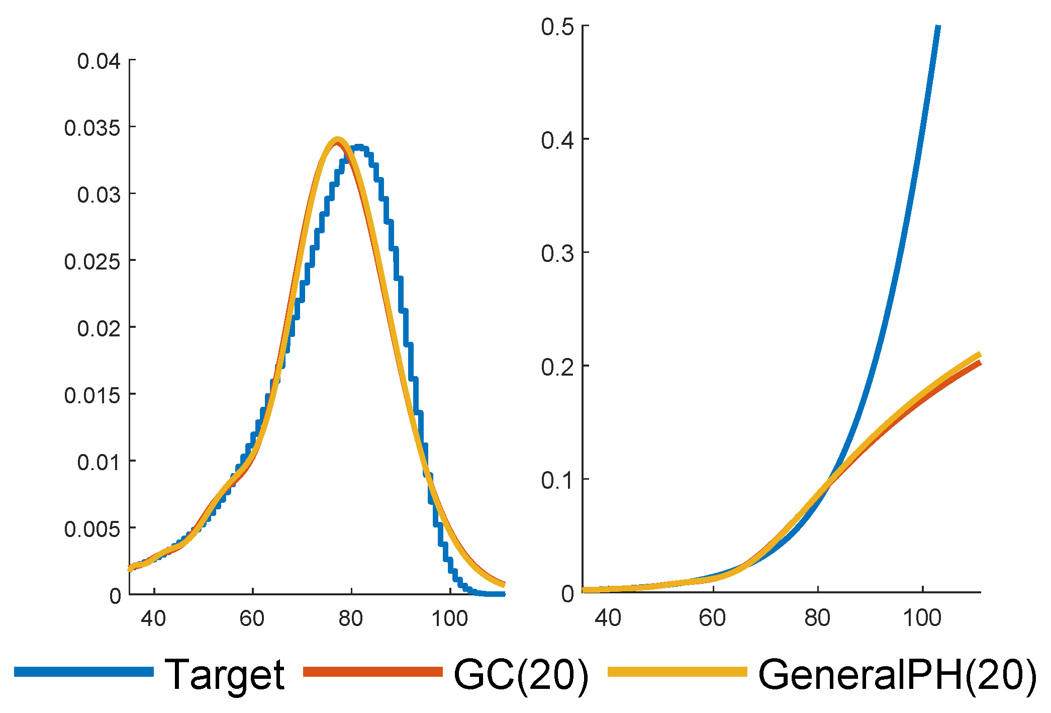
As a first illustration, we fit both a general structure PH and a generalized Coxian (GC) one with $p=20$ phases. The results are in Figure 3, with the densities of the fitted PH distributions in the left panel together with the data and the corresponding hazard rates in the right panel.

Figure 3. Probability density functions and hazard rate functions for the life table and phase-type (PH) fits using the general and the generalized Coxian (GC) structures with $p=20$ phases.

The fits of the two structures are almost identical (but the shape of the density is somewhat off the data, which indicates that a larger valuer of p could be appropriate). The general structure leads to a system of ODEs of dimension $q=p^2+p$, whereas the corresponding number for GC is only $q=2p-1$. Due to this curse of dimensionality and the marginal differences of the fits, we have only considered GC structures for higher values of p.

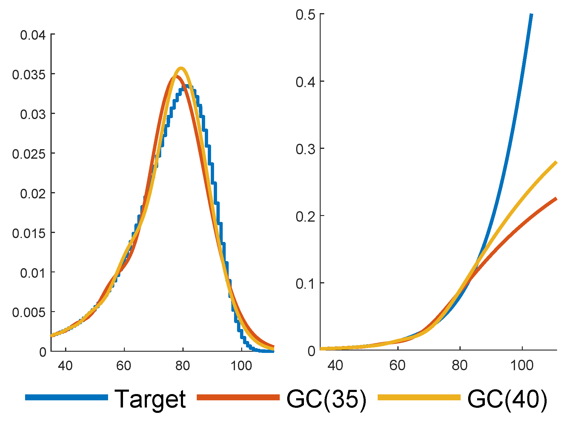
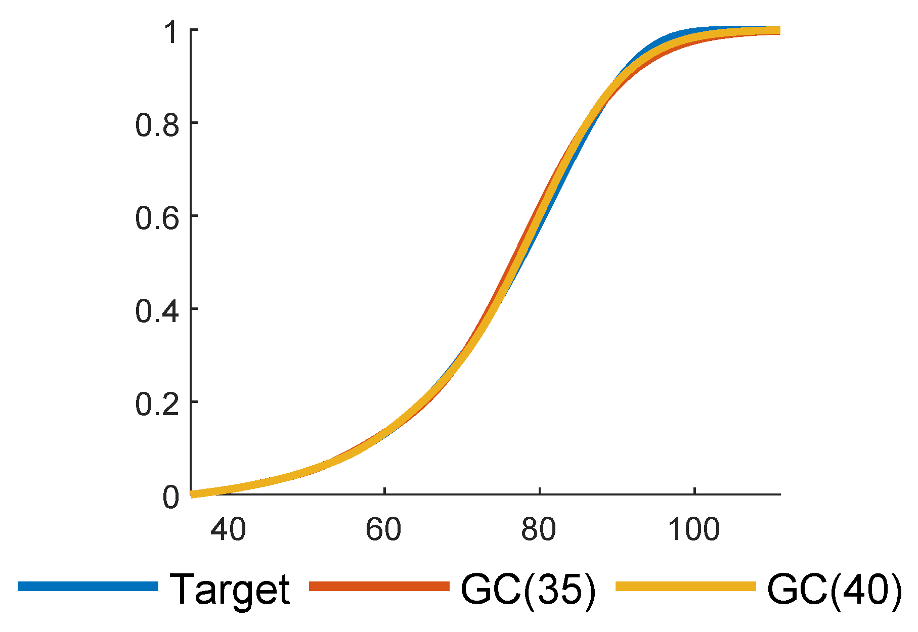
Figure 4 shows GC fits for $p=35$ and $p=40$. As expected, $p=40$ improves upon $p=35$.

Figure 4. Probability density functions and hazard rate functions for the life table and phase-type fits using the generalized Coxian structures with $p=35,40$ phases.

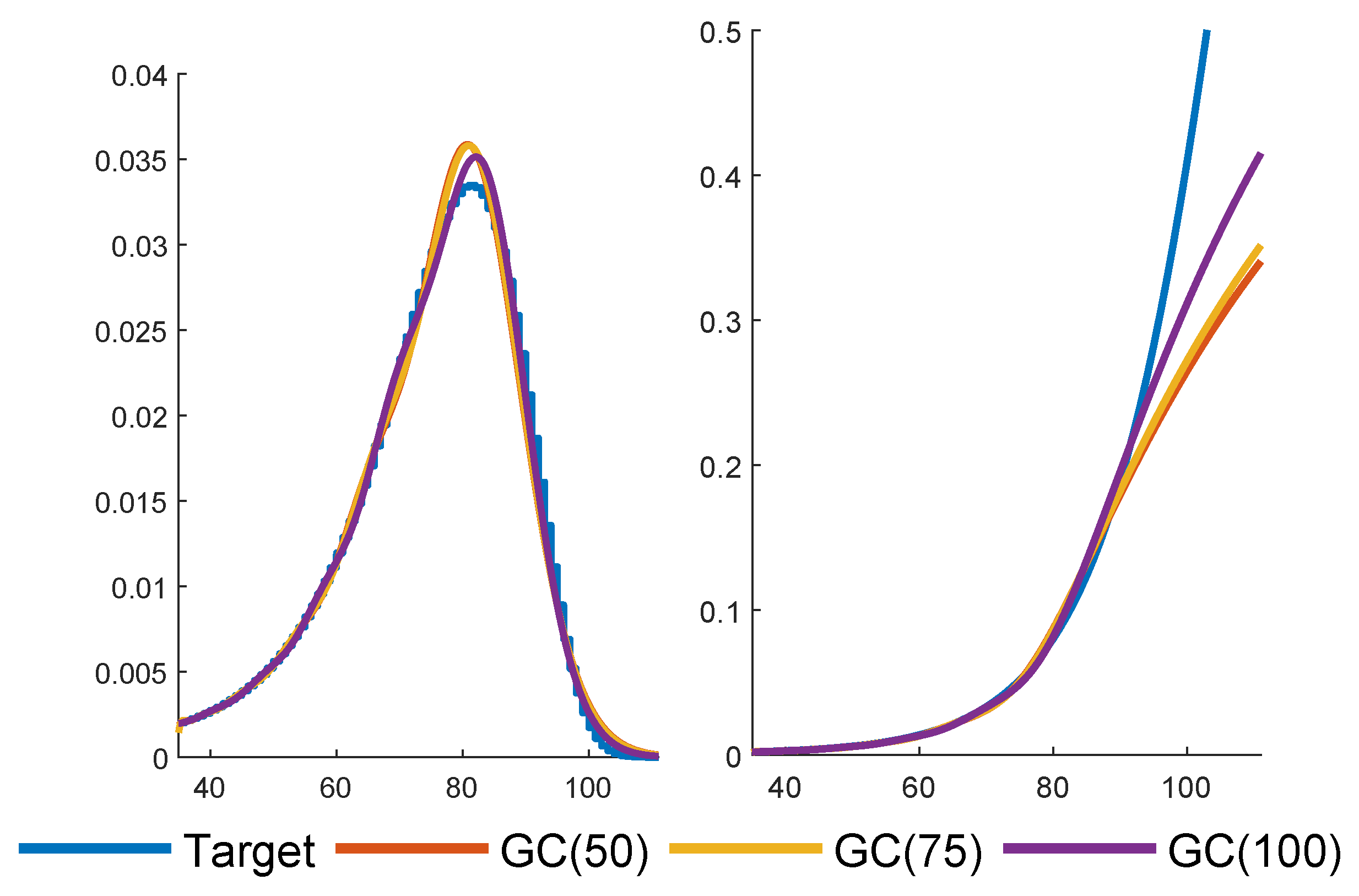
In Figure 5, we complement Figure 4 by plots of the tails. Such plots are frequently used to illustrate the quality of fits, but in our minds, a good agreement is not an argument in itself: two tails may come out quite similar in a comparison even if the shapes of the densities are rather different. Finally, Figure 6 gives GC fits with $p=50,75,100$.

Figure 5. Tails of the life table and GC fits with $p=35,40$ phases.

Figure 6. Probability density functions and hazard rate functions for the life table and GC fits with $p=50,75,100$ phases.

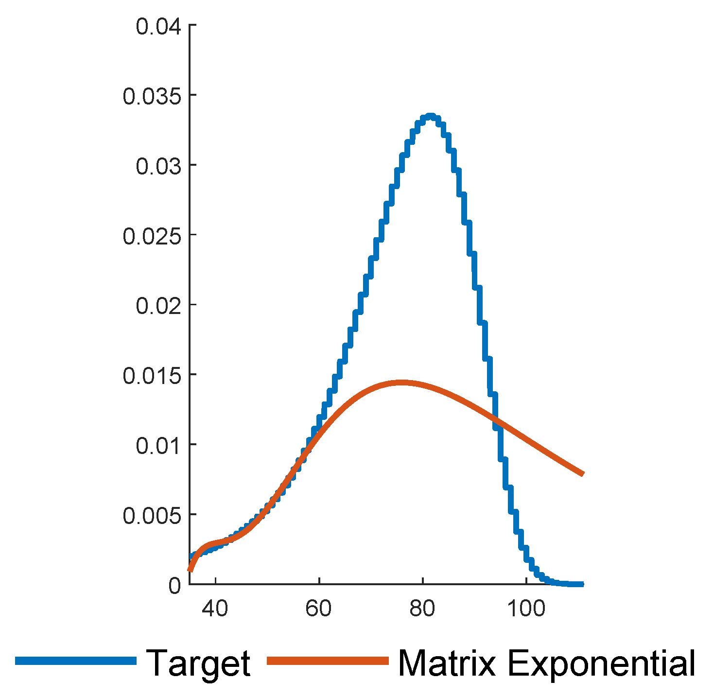
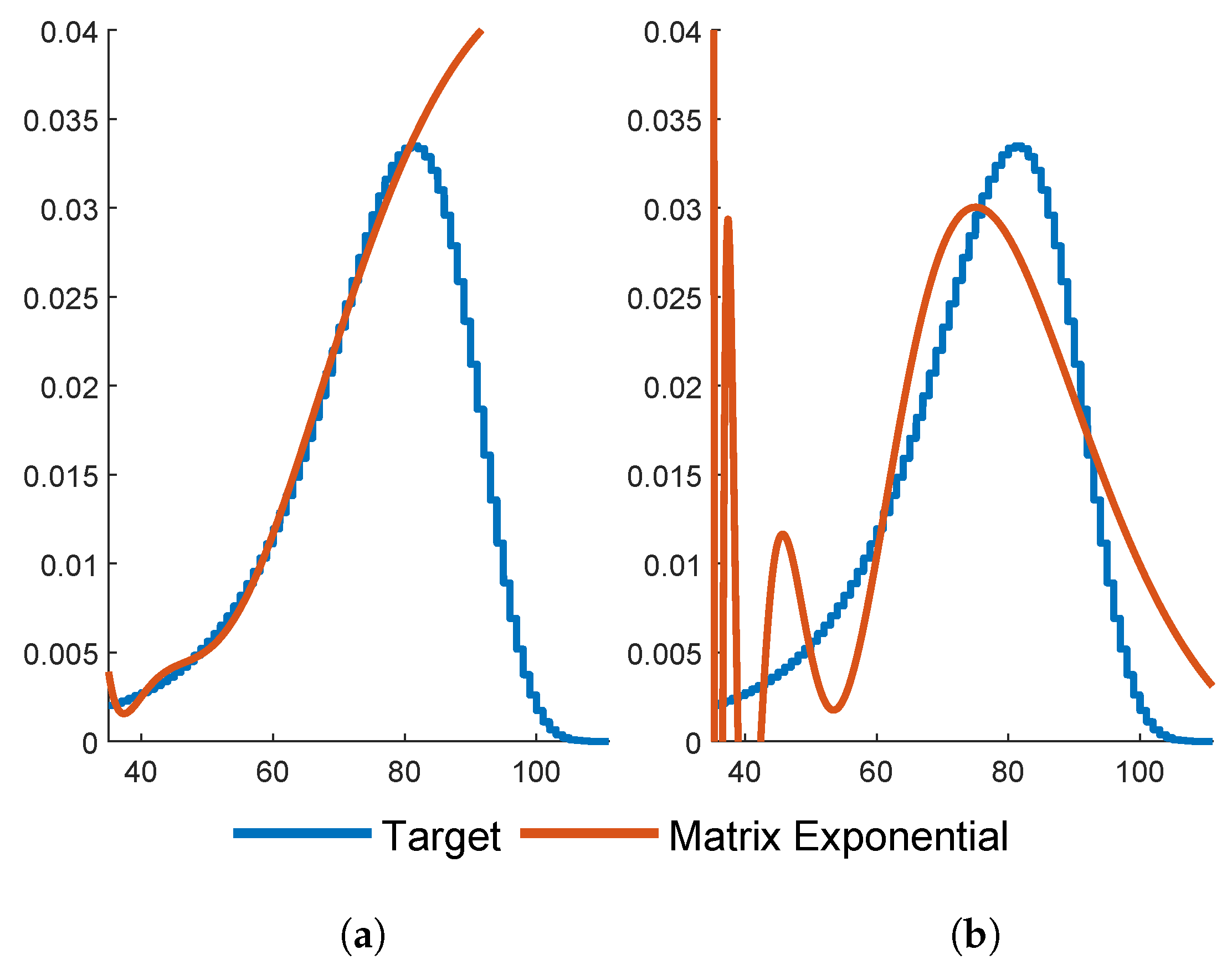
Which value of p should one then work with? There exists hardly a single criterion for answering such questions, i.e., assessing the quality of the fits to the data. Some concerns may be aesthetic, such as avoiding negative values of the density (cf. Appendix A below), support outside the obvious range of the data (cf. kernel estimates), or an excessive number of parameters (as is the case for most PH fits as compared to, e.g., the classical Gompertz-Makeham fit of life table data). Other concerns may have to do with the features of the distribution which are considered especially important, be it the overall shape of the density (caught well by maximum likelihood), the cumulative distribution function (c.d.f.), although c.d.f.’s may look close even for rather different distributions, the tail (where maximum likelihood fails and other tools such as the Hill estimator may be more appropriate), the hazard rate (as showing up in numerous life insurance contexts), or the behavior in a more narrow range (cf. a life insurance contract signed at the start of employment and running up to the time of retirement). For the present purposes and related ones like applications in queueing and insurance risk, the main point is, however, that PH fitting is not done for its own sake, but for the purpose of facilitating some calculation, here of the prices of equity-linked products, in queueing, say of waiting time characteristics, etc. In the rest of the paper, we therefore study the performance of the PH approach and the various fits and return to a discussion of the issue in the concluding Section 8.

4. Valuation of Benefits

The main application of the results in this paper is valuing equity-linked insurance products, in particular GMDBs in various deferred annuities. The time of payment of this kind of product is at the time $\tau$ of death of the policyholder, often denoted ${\tau }_x$, where x is his/her age at $t=0$ when he/she signs the contract. The amount of the payment depends on the price $S_{\tau }$ of a stock (or stock index) at that time and possibly also on the history of the stock price as, e.g., in (1). There are many different products (benefit functions) in the market. One example is the GMDB with benefit function being:

$$\mathrm{\Psi }({\overline{S}}_{\tau },S_{\tau })=max(S_{\tau },K)=S_{\tau }+{[K-S_{\tau }]}_{+},$$

(2)

where K is the guaranteed amount, e.g., $K=0.9S_0$. The second term on the right-hand side (r.h.s.) of (2) is the payoff of a life-contingent put option. Another popular product is the so-called high-water benefit (HWB) with the payoff function being:

$$\mathrm{\Psi }({\overline{S}}_{\tau },S_{\tau })={\overline{S}}_{\tau }.$$

Another form of the HWB function is:

$$\mathrm{\Psi }({\overline{S}}_{\tau },S_{\tau })=max(a{\overline{S}}_{\tau },S_{\tau })$$

where $0<a<1$. Since:

$$max(a{\overline{S}}_{\tau },S_{\tau })=S_{\tau }+max(a{\overline{S}}_{\tau }-S_{\tau },0),$$

(3)

the second term on the r.h.s. of (3) is the payoff of a life-contingent fractional lookback option.

In practice, the policyholders can withdraw. Note that the payment of the GMDB can be written as the payoff of a put option (plus a share of underlying stock). When the stock price rises, put options become less valuable; hence, policies may lapse. This motivates considering the benefit function:

$$\mathrm{\Psi }({\overline{S}}_{\tau },S_{\tau })=I_{\{{\overline{S}}_{\tau }<H\}}{[K-S_{\tau }]}_{+},$$

where $I_{\{.\}}$ is the indicator function and H is a “barrier”. This is a barrier option payoff form.

Since we can approximate the distribution of ${\tau }_x$ by a PH distribution, the valuation problem becomes calculating:

$$\mathbb{E}\left[{\mathrm{e}}^{-\delta \tau }\mathrm{\Psi }({\overline{S}}_{\tau },S_{\tau })\right],$$

(4)

where $\delta$ denotes a discounting factor and $\tau$ is PH r.v. One example is to take $\delta$ as the force of interest, but the company may want to use a lower $\delta$ in its technical reserve to ensure a conservative pricing.

5. The Factorization: Implementation for Jump Diffusions

Our basic assumption is that X is a jump diffusion with Brownian parameters $\mu ,{\sigma }^2$, upward jumps at rate ${\lambda }_1$ and with a PH$(p_1,{\mathit{\alpha }}_1,{\mathit{T}}_1)$ distribution of the sizes, and similar parameters ${\lambda }_2,p_2,{\mathit{\alpha }}_2,{\mathit{T}}_2$ for the downward jumps.

We will first need to introduce the equivalent time-reversed PH representation $({\mathit{\alpha }}^{*},{\mathit{T}}^{*})$ of $\tau$. It is obtained by considering:

$$J_t^{*}=\left\{\begin{array}{cc}{J}_{(\tau -t)-},\hfill & \mathrm{if}t<\tau ,\hfill \\ †,\hfill & \mathrm{otherwise}.\hfill \end{array}\right.$$

It turns out (Asmussen 2003, III.5) that $J^{*}$ is a terminating time-homogeneous Markov process with initial distribution ${\mathit{\alpha }}^{*}$ and generator ${\mathit{T}}^{*}$ given by:

$${\mathit{\alpha }}^{*}=\mathbb{E}\tau ·{\mathit{t}}^{\mathbf{\top }}{\Delta }_{\mathit{\nu }},{\mathit{T}}^{*}={\Delta }_{\mathit{\nu }}^{-1}{\mathit{T}}^{\mathbf{\top }}{\Delta }_{\mathit{\nu }},$$

(5)

where ${\Delta }_{\mathit{\nu }}$ denotes the diagonal matrix with the positive vector $\mathit{\nu }=-\mathit{\alpha }{\mathit{T}}^{-1}$ on the diagonal. To see this, consider a doubly-infinite stationary Markovian arrival process (Asmussen 2003, XI.1) with generator $\mathit{T}+\mathit{D}$, where $\mathit{D}=\mathit{t}\mathit{\alpha }$ gives the rates of phase changes with arrivals, and note that the corresponding stationary distribution of the phase process is proportional to $\mathit{\nu }$. Now, just use the standard time reversion for non-killed Markov processes. Considering, for the ease of exposition, the case $\delta =0$ of no discounting, the form of the factorization identity of (Asmussen and Ivanovs 2019) that is most convenient for our purposes is then:

$$\begin{array}{cc}\hfill \mathbb{P}(M_{\tau }\in \mathrm{d}x,D_{\tau }\in \mathrm{d}y)& =\sum _{k=1}^p\frac{1}{c_k}{\mathbb{P}}_{\mathit{\alpha }}^{*}(M_{\tau }\in \mathrm{d}x,J_{{\overline{\sigma }}_{\tau }}=k){\mathbb{P}}_{{\mathit{\alpha }}^{*}}^{*}(M_{\tau }\in \mathrm{d}y,J_{{\overline{\sigma }}_{\tau }}=k),\hfill \end{array}$$

(6)

where ${\mathbb{P}}^{*}$ is the probability measure where $\tau$ is generated by the time-reversed representation and X evolves as $-X$ did under $\mathbb{P}$, ${\overline{\sigma }}_{\tau }$ is the time at which the maximum is attained, and $c_k={\mathbb{P}}_{\mathit{\alpha }}(J_{{\overline{\sigma }}_{\tau }}=k)={\mathbb{P}}_{{\mathit{\alpha }}^{*}}^{*}(J_{{\overline{\sigma }}_{\tau }}=k)$.

The distributions of $M_{\tau },D_{\tau }$ are particularly simple if X is BM$(\mu ,{\sigma }^2)$ and $\tau$ exponential $\left(\lambda \right)$. In fact, they are then exponential with rates ${\rho }^{+}$, respectively ${\rho }^{-}$, where:

$${\rho }^{\pm }=\mp \frac{\mu }{{\sigma }^2}+\sqrt{\frac{{\mu }^2}{{\sigma }^4}+\frac{2\lambda }{{\sigma }^2}}.$$

If more generally, $X\left(t\right)$ is a jump diffusion with both up- and down-ward PH jumps, there is an abundance of results and algorithms giving the distributions in various representations or their Laplace transforms. See, among others, (Bean et al. 2005; Breuer 2008; Dieker and Mandjes 2011; Horváth and Telek 2017; Jacobsen 2005; Jiang and Pistorius 2008; Lewis and Mordecki 2008; Mordecki 2002; Pistorius 2006). The most appropriate form for our purposes is that for (computable) matrices $\mathit{U},{\mathit{U}}^{*}$ of dimension $p(1+p_1)\times p(1+p_1)$, respectively $p(1+p_2)\times p(1+p_2)$, one has:

$$\begin{array}{cc}\hfill {\mathbb{P}}_i\left(M_{\tau }\in \mathrm{d}x,J_{\overline{\sigma }}=k\right)& ={\mathit{e}}_i^{\mathbf{\top }}{\mathrm{e}}^{\mathit{U}x}{\mathit{e}}_k·u_k\hfill \end{array}$$

(7)

$$\begin{array}{cc}\hfill {\mathbb{P}}_j^{*}(M_{\tau }\in \mathrm{d}y,J_{{\overline{\sigma }}_{\tau }}=k)& ={\mathit{e}}_j^{\mathbf{\top }}{\mathrm{e}}^{{\mathit{U}}^{*}y}{\mathit{e}}_k·u_k^{*}\hfill \end{array}$$

(8)

where $u_k,u_k^{*}$ are the $k^{\mathrm{th}}$ element of the vectors $-\mathit{U}\mathit{e}$, respectively $-{\mathit{U}}^{*}\mathit{e}$; this occurs already in (Asmussen 1995), as well as several later sources, but we have in fact used a new and (we feel) somewhat more straightforward approach; see Appendix B.

Multiplying (7), (8) by ${\alpha }_i$, respectively ${\alpha }_j^{*}$ and summing over $i,j$, the factorization (6) then takes the form:

$$\begin{array}{c}\hfill \mathbb{P}(M_{\tau }\in \mathrm{d}x,D_{\tau }\in \mathrm{d}y)=\sum _{k=1}^p{r}_k·\mathit{\alpha }{\mathrm{e}}^{\mathit{U}x}{\mathit{e}}_k·{\mathit{\alpha }}^{*}{\mathrm{e}}^{-{\mathit{U}}^{*}y}{\mathit{e}}_k\end{array}$$

where $r_k=u_k{u}_k^{*}/c_k$. The modification with discounting is explained in Section 4 of (Asmussen and Ivanovs 2019) and becomes:

$$\begin{array}{c}\hfill \mathbb{E}[{\mathrm{e}}^{-\delta \tau };M_{\tau }\in \mathrm{d}x,D_{\tau }\in \mathrm{d}y]=\sum _{k=1}^p{r}_k·\mathit{\alpha }{\mathrm{e}}^{{\mathit{U}}_{\delta }x}{\mathit{e}}_k·{\mathit{\alpha }}^{*}{\mathrm{e}}^{-{\mathit{U}}_{\delta }^{*}y}{\mathit{e}}_k\end{array}$$

(9)

where ${\mathit{U}}_{\delta }$, ${\mathit{U}}_{\delta }^{*}$ are calculated as $\mathit{U},{\mathit{U}}^{*}$ with $\mathit{T}$ replaced by $\mathit{T}-\delta \mathit{I}$ (here, the $r_k$ remain unchanged, i.e., $u_k$, $u_k^{*}$ and $c_k$ are computed for the case $\delta =0$). This can be rewritten in matrix form as follows:

Corollary 1.

(i) For $x,y\ge 0$,

$$\begin{array}{c}\hfill \mathbb{E}[{\mathrm{e}}^{-\delta \tau };M_{\tau }\in \mathrm{d}x,D_{\tau }\in \mathrm{d}y]=\mathit{\alpha }{\mathrm{e}}^{{\mathit{U}}_{\delta }x}{\Delta }_r{\mathrm{e}}^{{{\mathit{U}}_{\delta }^{*}}^{\mathbf{\top }}y}{{\mathit{\alpha }}^{*}}^{\mathbf{\top }}={\mathit{\alpha }}^{*}{\mathrm{e}}^{{\mathit{U}}_{\delta }^{*}y}{\Delta }_r{\mathrm{e}}^{{{\mathit{U}}_{\delta }}^{\mathbf{\top }}x}{\mathit{\alpha }}^{\mathbf{\top }};\end{array}$$

(ii) For functions f and g,

$$\mathbb{E}\left[{\mathrm{e}}^{-\delta \tau }f\left(M_{\tau }\right)g\left(D_{\tau }\right)\right]=\mathit{\alpha }{\mathit{F}}_{{\mathit{U}}_{\delta }}{\Delta }_r{\mathit{G}}_{{\mathit{U}}_{\delta }^{*}}^{\mathbf{\top }}{{\mathit{\alpha }}^{*}}^{\mathbf{\top }}={\mathit{\alpha }}^{*}{\mathit{G}}_{{\mathit{U}}_{\delta }^{*}}{\Delta }_r{\mathit{G}}_{{\mathit{U}}_{\delta }}^{\mathbf{\top }}{\mathit{\alpha }}^{\mathbf{\top }}$$

where ${\mathit{F}}_{{\mathit{U}}_{\delta }}$, ${\mathit{G}}_{{\mathit{U}}_{\delta }^{*}}$ are the matrices ${\int }_0^{\infty }f\left(x\right){\mathrm{e}}^{{\mathit{U}}_{\delta }x}\mathrm{d}x$, respectively ${\int }_0^{\infty }g\left(y\right){\mathrm{e}}^{{\mathit{U}}_{\delta }^{*}y}\mathrm{d}y$.

Proof. 

Since ${\mathit{\alpha }}^{*}{\mathrm{e}}^{-{\mathit{U}}_{\delta }^{*}y}{\mathit{e}}_k\in {\mathbb{R}}^1$, it may be replaced by its transpose ${\mathit{e}}_k^{\mathbf{\top }}{\mathrm{e}}^{-{{\mathit{U}}_{\delta }^{*}}^{\mathbf{\top }}y}{{\mathit{\alpha }}^{*}}^{\mathbf{\top }}$ in (9), and this gives the first identity in (i); the second follows by transposition. Part (ii) then follows by integration. ▯

For computations, the matrix form rather than the sum form is convenient for keeping the code short and transparent, and in many software packages like MATLAB, it also is faster. In a number of our examples, the matrices ${\mathit{F}}_{\mathit{U}}$, ${\mathit{G}}_{{\mathit{U}}^{*}}$ come out in a simple form, avoiding integration. Here is a first example:

Example 1.

For the HWB, we need to compute:

$$\mathbb{E}\left[{\mathrm{e}}^{-\delta \tau }max(a{\overline{S}}_{\tau },S_{\tau })\right]=S_0\mathbb{E}\left[{\mathrm{e}}^{-\delta \overline{\tau }}{\mathrm{e}}^{M_{\tau }}·{\mathrm{e}}^{-\delta \underline{\tau }}max(a,{\mathrm{e}}^{-D_{\tau }})\right].$$

(10)

Thus (assuming $S_0=1$ w.l.o.g.), we have $f\left(x\right)={\mathrm{e}}^x$, $g\left(y\right)=max(a,{\mathrm{e}}^{-y})$ in Part (ii) of Corollary 1, and we get:

$$\begin{array}{cc}\hfill {\mathit{F}}_{{\mathit{U}}_{\delta }}& ={\int }_0^{\infty }{\mathrm{e}}^x{\mathrm{e}}^{{\mathit{U}}_{\delta }x}\mathrm{d}x=-{(\mathit{I}+{\mathit{U}}_{\delta })}^{-1},\hfill \\ \hfill {\mathit{G}}_{{\mathit{U}}_{\delta }^{*}}& =a{\int }_{-loga}^{\infty }{\mathrm{e}}^{{\mathit{U}}_{\delta }^{*}y}\mathrm{d}y+{\int }_0^{-loga}{\mathrm{e}}^{-y}{\mathrm{e}}^{{\mathit{U}}_{\delta }^{*}y}\mathrm{d}y\hfill \\ & =-a{\mathrm{e}}^{-{\mathit{U}}_{\delta }^{*}loga}{{\mathit{U}}_{\delta }^{*}}^{-1}+(\mathit{I}-a{\mathrm{e}}^{-{\mathit{U}}_{\delta }^{*}loga}){(\mathit{I}-{\mathit{U}}_{\delta }^{*})}^{-1}.\hfill \end{array}$$

 ⋄

Corollary 2.

Define ${\displaystyle {\mathit{S}}_{\delta }={\int }_0^{\infty }{\mathrm{e}}^{{\mathit{U}}_{\delta }y}{\Delta }_r{\mathrm{e}}^{{{\mathit{U}}_{\delta }^{*}}^{\mathbf{\top }}y}\mathrm{d}y}$. Then:

$$\mathbb{E}[{\mathrm{e}}^{-\delta \tau };X_{\tau }\in \mathrm{d}x]=\left\{\begin{array}{cc}\mathit{\alpha }{\mathrm{e}}^{{\mathit{U}}_{\delta }x}{\mathit{S}}_{\delta }{{\mathit{\alpha }}^{*}}^{\mathbf{\top }}\hfill & forx>0\hfill \\ {\mathit{\alpha }}^{*}{\mathrm{e}}^{-{\mathit{U}}_{\delta }^{*}x}{\mathit{S}}_{\delta }^{\mathbf{\top }}{\mathit{\alpha }}^{\mathbf{\top }}\hfill & forx<0.\hfill \end{array}\right.$$

Proof. 

For $x>0$, we have:

$$\mathbb{E}[{\mathrm{e}}^{-\delta \tau };X_{\tau }\in \mathrm{d}x]={\int }_0^{\infty }\mathbb{E}[{\mathrm{e}}^{-\delta \tau };M_{\tau }\in \mathrm{d}x+y,D_{\tau }\in \mathrm{d}y],$$

and so, the result follows immediately by Part (ii) of Corollary 1. The proof for $x<0$ is similar; one only has to note that if ${\mathit{S}}_{\delta }^{*}$ is defined as ${\mathit{S}}_{\delta }$ with ${\mathit{U}}_{\delta }$ and ${\mathit{U}}_{\delta }^{*}$ interchanged, then ${\mathit{S}}_{\delta }^{*}={\mathit{S}}_{\delta }^{\mathbf{\top }}$. ▯

Remark 2.

The distribution of $X_{\tau }$ restricted to $(0,\infty )$ is in fact (defective) PH, but in general, with a different generator $\tilde{\mathit{U}}$ than $\mathit{U}={\mathit{U}}_0$ (for this one would have needed that ${\mathit{S}}_{\delta }{{\mathit{\alpha }}^{*}}^{\mathbf{\top }}$ be proportional to $-\mathit{U}\mathit{e}$). This follows from the general fact that if $\mathit{\alpha },\mathit{s}\ge 0$ and $\mathit{T}$ is a phase generator, but possibly $\mathit{s}\ne -\mathit{T}\mathit{e}$, then $\mathit{\alpha }{\mathrm{e}}^{\mathit{T}x}\mathit{s}=\tilde{\mathit{\alpha }}{\mathrm{e}}^{\tilde{\mathit{T}}x}\tilde{\mathit{t}}$ where:

$$\tilde{\mathit{\alpha }}=\mathit{\alpha }{\Delta }_v,\tilde{\mathit{T}}={\Delta }_v^{-1}\mathit{T}{\Delta }_v,\tilde{\mathit{t}}=-\tilde{\mathit{T}}\mathit{e}={\Delta }_v^{-1}\mathit{s}\mathrm{with}\mathit{v}=-{\mathit{T}}^{-1}\mathit{s},$$

and here, $\tilde{\mathit{T}}$ is a phase generator; all needed positivity properties follow from ${\mathit{S}}_{\delta }$ and $-{\mathit{T}}^{-1}$ being non-negative.

Similar remarks apply to the negative part of $X_{\tau }$. These observations may be seen as an extension to jump diffusions at PH times of the standard fact that Brownian motion at an independent exponential time has a two-sided exponential distribution (often called the Laplace distribution). A similar result for matrix-exponential distributions is on p. 478 of (Bladt and Nielsen 2017), but is in terms of Laplace transforms rather than densities.

Example 2.

For the GMDB, the price is (taking $S_0=1$):

$$\begin{array}{c}\hfill \mathbb{E}[{\mathrm{e}}^{-\delta \tau }max(S_{\tau },K)]=K\mathbb{E}[{\mathrm{e}}^{-\delta \tau };X_{\tau }\le logK]+\mathbb{E}[{\mathrm{e}}^{-\delta \tau +X_{\tau }};X_{\tau }>logK].\end{array}$$

In the most common case $K<S_0$, the first term equals:

$$\begin{array}{c}\hfill K{\int }_{-\infty }^{logK}{\mathit{\alpha }}^{*}{\mathrm{e}}^{-{\mathit{U}}_{\delta }^{*}x}{\mathit{S}}_{\delta }^{\mathbf{\top }}{\mathit{\alpha }}^{\mathbf{\top }}\mathrm{d}x=-K{\mathit{\alpha }}^{*}{{\mathit{U}}_{\delta }^{*}}^{-1}{\mathrm{e}}^{-{\mathit{U}}_{\delta }^{*}logK}{\mathit{S}}_{\delta }^{\mathbf{\top }}{\mathit{\alpha }}^{\mathbf{\top }}\end{array}$$

when $S_0=1$, whereas the second is:

$$\begin{array}{c}{\int }_{logK}^0{\mathrm{e}}^x{\mathit{\alpha }}^{*}{\mathrm{e}}^{-{\mathit{U}}_{\delta }^{*}x}{\mathit{S}}_{\delta }^{\mathbf{\top }}{\mathit{\alpha }}^{\mathbf{\top }}\mathrm{d}x+{\int }_0^{\infty }{\mathrm{e}}^x\mathit{\alpha }{\mathrm{e}}^{{\mathit{U}}_{\delta }x}{\mathit{S}}_{\delta }{{\mathit{\alpha }}^{*}}^{\mathbf{\top }}\mathrm{d}x\hfill \\ ={\mathit{\alpha }}^{*}{(\mathit{I}-{\mathit{U}}_{\delta }^{*})}^{-1}\left(\mathit{I}-K{\mathrm{e}}^{-{\mathit{U}}_{\delta }^{*}logK}\right){\mathit{S}}_{\delta }^{\mathbf{\top }}{\mathit{\alpha }}^{\mathbf{\top }}-\mathit{\alpha }{(\mathit{I}+{\mathit{U}}_{\delta })}^{-1}{\mathit{S}}_{\delta }{{\mathit{\alpha }}^{*}}^{\mathbf{\top }}.\hfill \end{array}$$

 ⋄

Example 3.

The calculation of reserves:

$$V_t=\mathbb{E}\left[{\mathrm{e}}^{-\delta (\tau -t)}\mathrm{\Phi }(M_{\tau },D_{\tau })|X_s,0\le s\le t,\tau >t\right]$$

is closely related to price calculations. However, the details may be somewhat more cumbersome since for a fixed t, the expressions for $M_{\tau },D_{\tau }$ have two components, the quantities $m_0={max}_{s\le t}{X}_s$ and $d_0=m_0-X_t$, which are known at time t, and the unknown random ones:

$$m_1=\underset{t\le s<\tau }{max}(X_s-X_t),d_1=m_1-x_1\mathrm{where}{x}_1=X_{\tau }-X_t.$$

In terms of these and the relations:

$$\begin{array}{cc}\hfill M_{\tau }& =max(m_0,x_0+m_1),\hfill \\ \hfill D_{\tau }& =max(m_0,x_0+m_1)-x_0-x_1=max(d_0,d_1)-x_1\hfill \\ & ={[d_0-m_1]}^{+}+d_1,\hfill \end{array}$$

we can write $\mathrm{\Phi }(M_{\tau },D_{\tau })=\tilde{\mathrm{\Phi }}(m_1,d_1)$, where:

$$\tilde{\mathrm{\Phi }}(x,y)=\mathrm{\Phi }\left(max(m_0,x_0+x),{[d_0-x]}^{+}+y\right).$$

Since the conditional distribution of $\tau -t$ given $\tau >t$ is PH$({\mathit{\alpha }}_t,\mathit{T})$ where ${\mathit{\alpha }}_t=\mathit{\alpha }{\mathrm{e}}^{\mathit{T}t}/\mathit{\alpha }{\mathrm{e}}^{\mathit{T}t}\mathit{e}$, this gives:

$$V_t={\int }_0^{\infty }{\int }_0^{\infty }\tilde{\mathrm{\Phi }}(x,y){\mathit{\alpha }}_t{\mathrm{e}}^{{\mathit{U}}_{\delta }x}{\Delta }_r{\mathrm{e}}^{{{\mathit{U}}_{\delta }^{*}}^{\mathbf{\top }}y}{{\mathit{\alpha }}^{*}}^{\mathbf{\top }}\mathrm{d}y\mathrm{d}x$$

(11)

(note that for the reversal, we need not calculate ${\mathit{\alpha }}^{*}$ by replacing $\mathit{\alpha }$ by ${\mathit{\alpha }}_t$ in (5), but can use the same ${\mathit{\alpha }}^{*}$ for all t, cf. Section 2.2 of (Asmussen and Ivanovs 2019)).

Example 4.

For the GMDB, we have:

$$\mathrm{\Phi }(M_{\tau },D_{\tau })=max(K,{\mathrm{e}}^{X_{\tau }})=max(K,{\mathrm{e}}^{x_0+x_1})={\mathrm{e}}^{x_0}max(\tilde{K},{\mathrm{e}}^{x_1})$$

where $\tilde{K}=K{\mathrm{e}}^{-x_0}$. Combining with Remark 2, we therefore arrive at the same expression as in Example 2 when $K{\mathrm{e}}^{-x_0}\le 1$, only with K replaced by $\tilde{K}$ and $\mathit{\alpha }$ by ${\alpha }_t$. The case $K{\mathrm{e}}^{-x_0}>1$ may arise by randomness, but is just a minor modification.

Example 5.

The details for the HWB reserves are somewhat more complicated than for the GMDB. Here, one needs to consider ${\mathrm{e}}^{M_{\tau }}max(a,{\mathrm{e}}^{-D_{\tau }})$, corresponding to:

$$\tilde{\mathrm{\Phi }}(x,y)=exp\left\{max(m_0,x_0+m_1)\right\}max(a,exp\left\{-{[d_0-m_1]}^{+}-d_1\right\}.$$

One approach (potentially the easier one) may be simply to insert in (11) and do the two-dimensional numerical integration. However, in fact, one can reduce to a one-dimensional numerical integration similar to Corollary 2. To this end, note that ${\mathrm{e}}^{M_{\tau }}max(a,{\mathrm{e}}^{-D_{\tau }})$ after simple derivations comes out as:

$$\{\begin{array}{lll}{\mathrm{e}}^{x_0+m_1}a& \mathrm{if}\hspace{1em}{m}_1>d_0,d_1>-loga,& \left(12\mathrm{a}\right)\\ {\mathrm{e}}^{x_0+m_1-d_1}& \mathrm{if}\hspace{1em}{m}_1>d_0,d_1\le -loga,& \left(12\mathrm{b}\right)\\ {\mathrm{e}}^{m_0\mathrm{a}}& \mathrm{if}\hspace{1em}{m}_1\le d_0,d_0-m_1+d_1>-loga,& \left(12\mathrm{c}\right)\\ {\mathrm{e}}^{m_0}{\mathrm{e}}^{-d_0+m_1-d_1}& \mathrm{if}\hspace{1em}{m}_1\le d_0,d_0-m_1+d_1\le -loga.& \left(12\mathrm{d}\right)\end{array}$$

of these four possibilities, (12d) (and to a slightly lesser extent, (12c)) is the most complicated one with which to deal. The contribution to the reserve from (12c) is zero if $m_0<d_0+loga$, since then, the defining region is empty. Otherwise, it becomes:

$${\mathrm{e}}^{-\delta t+m_0-d_0}\underset{m_0+loga}{\overset{d_0}{\int }}\underset{0}{\overset{x-d_0-loga}{\int }}{\mathrm{e}}^{x-y}{\mathit{\alpha }}_t{\mathrm{e}}^{{\mathit{U}}_{\delta }x}{\Delta }_r{\mathrm{e}}^{{{\mathit{U}}_{\delta }^{*}}^{\mathbf{\top }}y}{{\mathit{\alpha }}^{*}}^{\mathbf{\top }}\mathrm{d}y\mathrm{d}x$$

which after two integrations reduces to an expression, which, though complicated, only involves known matrices and their exponentials, except that:

$${\mathit{S}}_{\delta }(b,c)={\int }_b^c{\mathrm{e}}^{{\mathit{U}}_{\delta }x}{\Delta }_r{\mathrm{e}}^{{{\mathit{U}}_{\delta }^{*}}^{\mathbf{\top }}x}\mathrm{d}x$$

is left to be determined by numerical integration. ⋄

6. Numerical Examples

For the underlying stock price process $S_t=S_0{\mathrm{e}}^{X_t}$, the most popular model is the geometric Brownian motion model. Since this model cannot capture the asymmetric leptokurtic features and the volatility smile, many modified models have been proposed in the literature; one of these is the jump diffusion model, cf. (Kou 2002). Empirical studies show that the daily return distribution tends to have larger kurtosis than the distribution of monthly returns, and the jump diffusion model can capture this feature; see (Das and Foresi 1996). As an illustrative example, we suppose that the yearly interest rate is $r=3\%$ and the yearly volatility $\sigma =0.25$. The jumps follow a compound Poisson process with upward jump rate ${\lambda }_1=3$ with the jump sizes being exponential with rate ${\nu }_1=50$ (mean 1/50) and downward jump rate ${\lambda }_2=2$ with jump size being exponential with rate ${\nu }_2=30$. When considering the valuation of an insurance product alone, it is not necessary to use a risk-neutral valuation approach. However, since in our setting, the underlying involves an equity, it is natural to use an equivalent martingale measure $\mathbb{Q}$, defined by the requirement $log{\mathbb{E}}_{\mathbb{Q}}{\mathrm{e}}^{X\left(1\right)}=r$. This does not define $\mathbb{Q}$ uniquely since the market is incomplete due to the jumps and the mortality risk. Our choice was to let the parameters ${\sigma }^2,{\lambda }_1,{\lambda }_2,{\nu }_1,{\nu }_2$ remain unchanged, which gives the risk-neutral Brownian drift as:

$$\mu =r-\frac{{\sigma }^2}{2}-\frac{{\lambda }_1}{{\nu }_1-1}+\frac{{\lambda }_2}{{\nu }_2+1}.$$

For the illustrative example, we have:

$$\mu =0.03-\frac{{0.25}^2}{2}-\frac{3}{50-1}+\frac{2}{30+1}=0.002042.$$

It is left to compute the ${\mathit{U}}_{\delta },{\mathit{U}}_{\delta }^{*}$. Writing:

$$\mathit{U}=\mathit{U}(\mathit{T},\mu ,{\sigma }^2,{\lambda }_1,{\lambda }_2,{\nu }_1,{\nu }_2)$$

we obtain:

$${\mathit{U}}^{*}=\mathit{U}({\mathit{T}}^{*},-\mu ,{\sigma }^2,{\lambda }_2,{\lambda }_1,{\nu }_2,{\nu }_1),{\mathit{U}}_{\delta }=\mathit{U}(\mathit{T}-\delta \mathit{I},\mu ,{\sigma }^2,{\lambda }_1,{\lambda }_2,{\nu }_1,{\nu }_2),$$

and thus, it suffices to consider $\mathit{U}$. Essentially, two types of algorithms are available. One set is based on finding roots in the complex plane of equations of the form $\kappa \left(s\right)=a$ where $\kappa \left(s\right)=log\mathbb{E}{\mathrm{e}}^{sX\left(1\right)}$ is the Lévy exponent of X. The other uses fixed-point equations of the form $\mathit{U}=\psi \left(\mathit{U}\right)$ and iteration, $\mathit{U}={lim}_{n\to \infty }{\mathit{U}}_n$, with ${\mathit{U}}_n=\psi \left({\mathit{U}}_{n-1}\right)$ and ${\mathit{U}}_0$ suitably chosen.

We give a few examples of previous algorithms of both types in Appendix B. When implementing these with $\tau$ having one of the GC representations fitted in Section 3, our experience was that the root-finding method was only feasible for a rather small number p of phases. More precisely, for $p=50$ or $p=75$, meaningless results were produced, with warnings of the matrix $\mathit{H}$ being close to singular. This is understandable since many eigenvalues of the relevant matrices are almost identical. Since the iterative algorithms ran without problems also for large values of p, we have therefore concentrated on these. In fact, we have developed a new iterative algorithm, which may be simpler than previous ones. It is presented in Appendix B, but for now, we concentrate on some numerical examples.

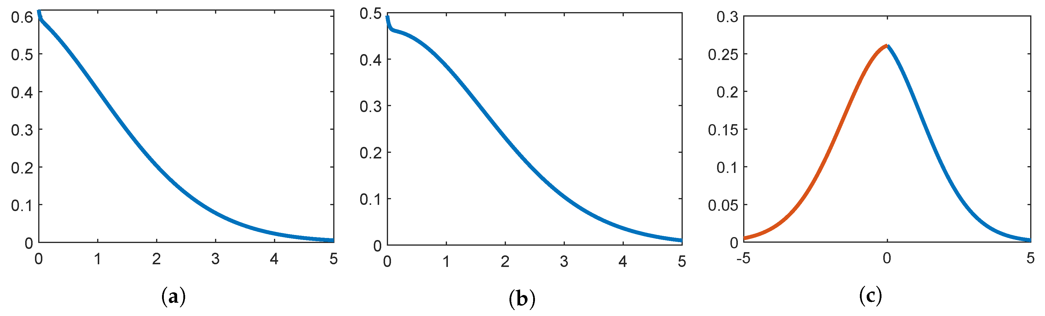
Example 6.

In Figure 7, we have plotted the marginal densities of $M_{\tau }$, $D_{\tau }$, and $X_{\tau }$.

Figure 7. Densities of (a) $M_{\tau }$, (b) $D_{\tau }$, and (c) $X_{\tau }$.

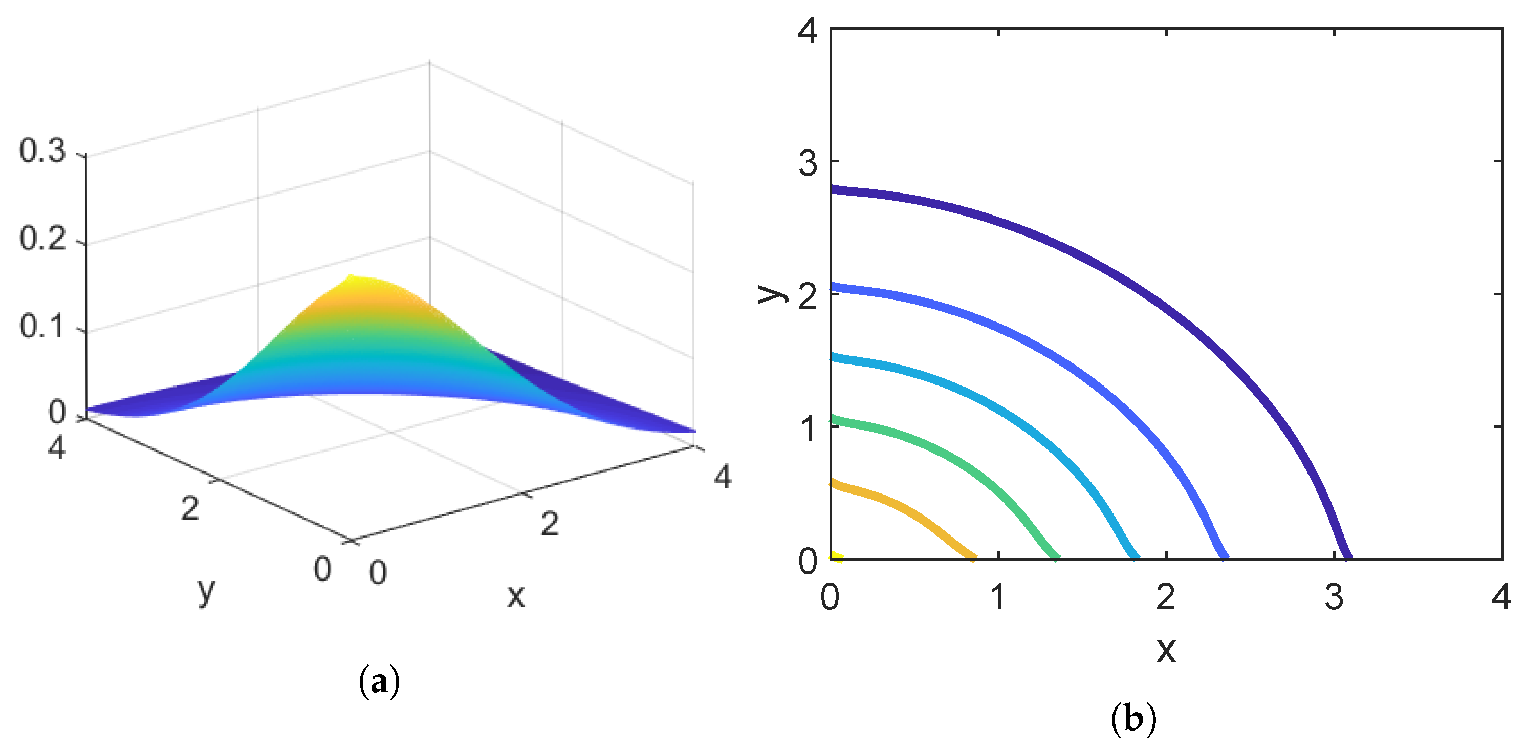
Example 7.

Figure 8 gives the joint distribution of $M_{\tau }$ and $D_{\tau }$ (computed by Corollary 1) for our jump diffusion with the parameters given above.

Figure 8. Joint distribution of $M_{\tau }$ and $D_{\tau }$. The joint density is in the left panel and a contour plot in the right.

Example 8.

To consider the sensitivity of the algorithms to the value p of chosen phases for $\tau$, we took $\delta =r=0.03$ or 0.00 and computed the price (10) for $p=$ 20, 35, 40, 50, 75, 100 and the GC fits presented in Section 3 for two products, the HWB with $a=0.85$ and the GMDB with $K=0.85$; the relevant formulas are available from Examples 1 and 2. The results are in Table 1. We also complemented with a Monte Carlo simulation estimate with an associated 95% confidence interval based on $R={10}^6$ replications, where $\tau$ was generated from the discrete life table distribution with an additional randomization within the year.

Table 1. Price estimates for $\delta =r$ and varying p. HWB, high-water benefit; GMDB, guaranteed minimum death benefit.

p	20	35	40	50	75	100	Monte Carlo
HWB, $\delta =r=0$	2.703	2.703	2.704	2.704	2.704	2.704	2.665 ± 0.008
HWB, $\delta =r=0.03$	1.698	1.699	1.699	1.699	1.699	1.699	1.680 ± 0.008
GMDB, $\delta =r=0$	1.468	1.468	1.468	1.468	1.468	1.468	1.467 ± 0.008
GMDB, $\delta =r=0.03$	1.080	1.080	1.079	1.079	1.079	1.079	1.079 ± 0.010

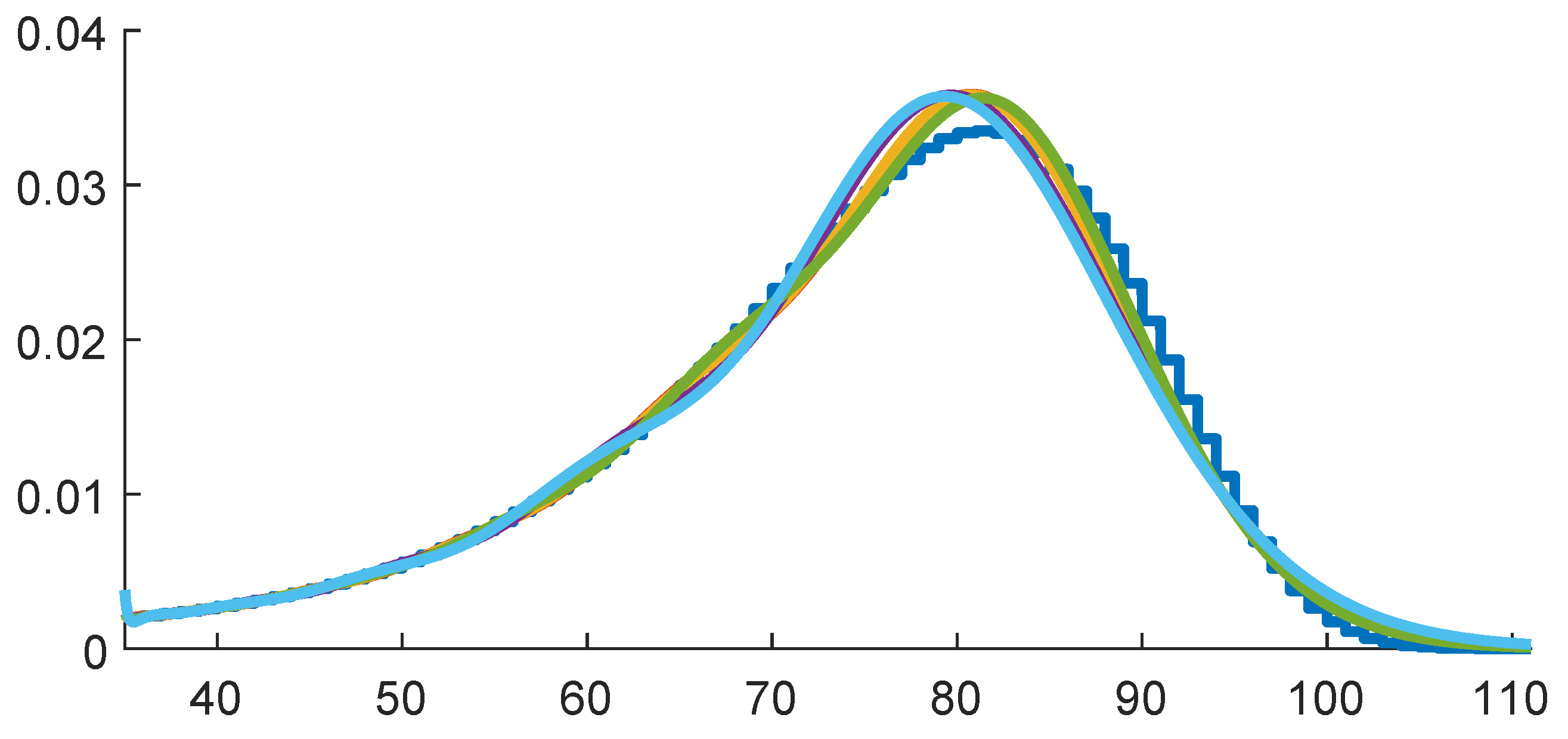
A related question is how varying different fits can be for a fixed p due to issues such as non-uniqueness of PH representations and possibly local maxima of the likelihood. We illustrate this point in Table 2, which is a parallel of Table 1. We fix p at 50, but use five different initial values (seeds) for the EM algorithm, all allowed the same running time. The fitted densities are in Figure 9.

Table 2. Price estimates for $\delta =r$ and varying seeds.

Seed	1	2	3	4	5	Monte Carlo
HWB, $\delta =r=0$	2.704	2.704	2.703	2.702	2.704	2.665 ± 0.008
HWB, $\delta =r=0.03$	1.699	1.699	1.699	1.698	1.699	1.680 ± 0.008
GMDB, $\delta =r=0$	1.468	1.468	1.468	1.467	1.468	1.467 ± 0.008
GMDB, $\delta =r=0.03$	1.079	1.079	1.079	1.078	1.080	1.079 ± 0.010

Figure 9. Fitted densities for five different seeds (against the life table data).

Our conclusion is that the differences are too minor to be of any concern, and certainly, using a single fit with $p\ge 50$ will produce acceptable results. Insisting on more than 2–3-digit precision in price estimates does not make sense due to issues such as model uncertainty and that payments will be adjusted later via bonus and dividend arrangements.

The programming was done in MATLAB on a 2014 MacBook Air with a 1.4 GHz Intel Core i5 processor. As an example of execution times, MATLAB’s tic-toc command reported approximately two seconds for each HWB or GMDB value using the PH methodology. The figures for the Monte Carlo values were much higher, approximately 30,000 replications per minute (recall that ${10}^6$ replications were used). The programming is very simple, with the main effort lying in writing a routine for computing $\mathit{U}$ for a given set of input parameters. This amounted to 50 lines of code in our implementation. Given this ease, we did some further price computations, even if our aim here is not to illustrate pricing aspects, but rather the computational ones.

Example 9.

We first consider varying the discount rate $\delta$, but not the force of interest r, cf. the remarks following (4) (that in particular motivate taking $\delta \le r$). The results for the HWB are in Table 3 and show the expected picture, that the price is decreasing in the discount rate.

Table 3. HWB price estimates for $r=0.03$ and varying $\delta$.

$\mathit{\delta }$	0.00	0.01	0.02	0.03
Price	6.24	3.99	2.58	1.70

Example 10.

The next example is discounting with the force of interest, i.e., taking $r=\delta$ and varying r. The numerical values are in Table 4, and the picture is again that the price is decreasing in $r=\delta$. The intuition is less clear-cut here, since the Brownian drift $\mu$ is increasing and thus pulls in the opposite direction.

Table 4. HWB price estimates for varying $r=\delta$.

$\mathit{r}\mathbf{=}\mathit{\delta }$	0.00	0.01	0.02	0.03	0.05
Price	2.70	2.23	1.92	1.70	1.44

Example 11.

Next, we give an illustration of a feature of the factorization: if $\tau$ is exponential, then $M_{\tau }$ and $D_{\tau }$ are independent. cf. Lemma 1. In the PH case, there is dependence caused by the common value of $\overline{\tau }=k$. How does this influence the price? A numerical illustration is in Table 5, where the entries are the ratios between the correct price with dependence and the incorrect one computed assuming independence, i.e., as:

$$\begin{array}{c}\mathbb{E}{\mathrm{e}}^{-\delta \overline{\tau }}{\mathrm{e}}^{M_{\tau }}·\mathbb{E}{\mathrm{e}}^{-\delta \underline{\tau }}max(a,{\mathrm{e}}^{-D_{\tau }})\hfill \\ ={\int }_0^{\infty }{\mathrm{e}}^x\mathit{\alpha }{\mathrm{e}}^{{\mathit{U}}_{\delta }x}\mathit{u}\mathrm{d}x·\left(a{\int }_{-loga}^{\infty }{\mathit{\alpha }}^{*}{\mathrm{e}}^{{\mathit{U}}_{\delta }^{*}y}{\mathit{u}}^{*}\mathrm{d}y+{\int }_0^{-loga}{\mathrm{e}}^{-y}{\mathit{\alpha }}^{*}{\mathrm{e}}^{{\mathit{U}}_{\delta }^{*}y}{\mathit{u}}^{*}\mathrm{d}y\right)\hfill \\ =-\mathit{\alpha }{(\mathit{I}+{\mathit{U}}_{\delta })}^{-1}\mathit{u}\left(-a{\mathit{\alpha }}^{*}{\mathrm{e}}^{-{\mathit{U}}_{\delta }^{*}loga}{{\mathit{U}}_{\delta }^{*}}^{-1}{\mathit{u}}^{*}+{\mathit{\alpha }}^{*}(\mathit{I}-a{\mathrm{e}}^{-{\mathit{U}}_{\delta }^{*}loga}){(\mathit{I}-{\mathit{U}}_{\delta }^{*})}^{-1}{\mathit{u}}^{*}\right).\hfill \end{array}$$

Table 5. Ratios between prices with and without dependence.

$\mathit{\delta }$	0.00	0.01	0.02	0.03	0.05
Ratio	0.97	0.88	0.78	0.68	0.51

The other settings are as in Table 3. Table 5 shows that in some cases, dependence indeed influences the price quite a bit.

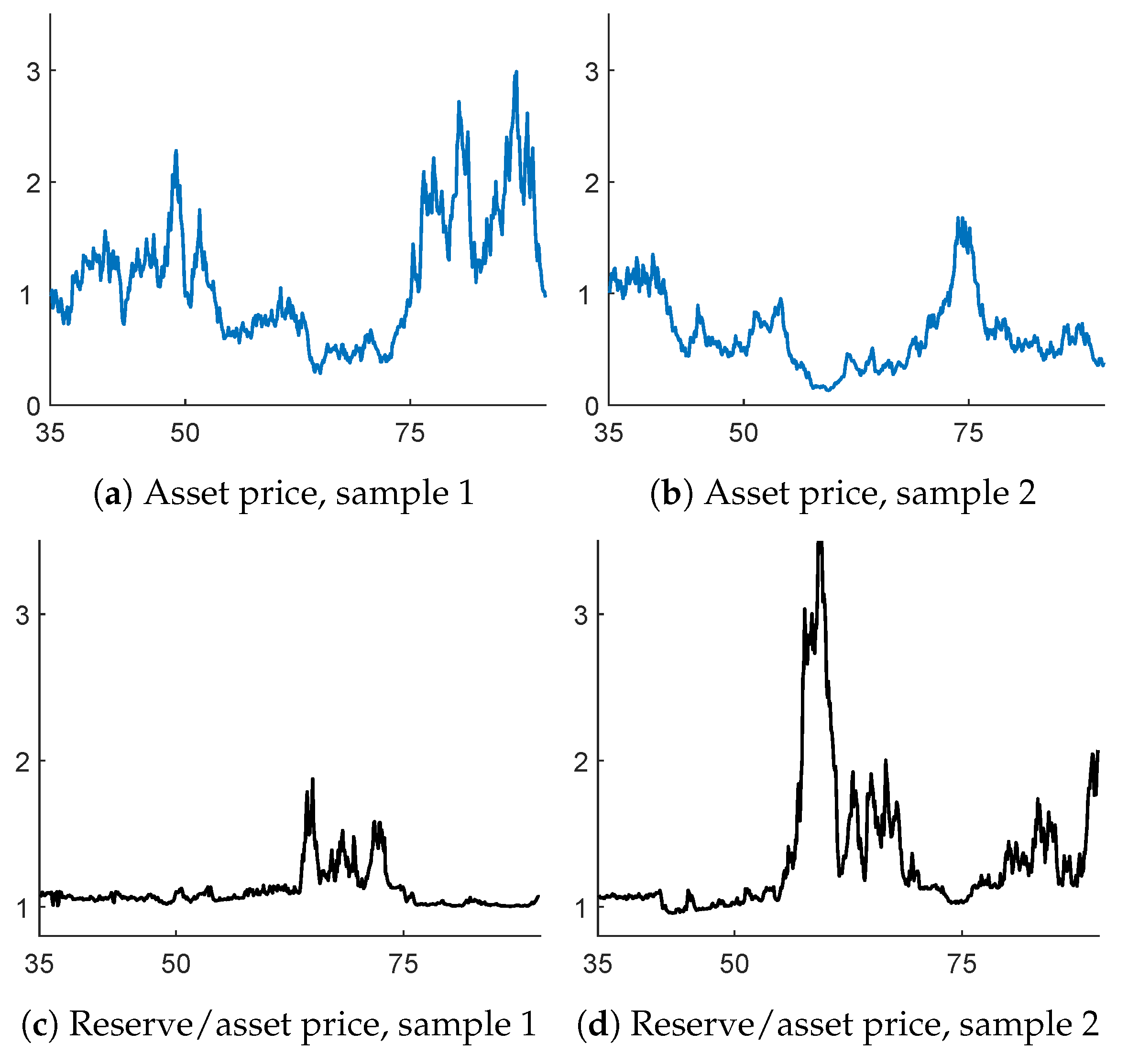
Example 12.

As a follow-up of Example 3, we finally consider the evaluation of reserves. Two paths of the jump diffusion were simulated, and the reserve was calculated for each value of t using the formulas of Examples 3, 4 and 5. The results are given in the graphs of Figure 10. The upper panel gives the stock price $S_{a-35}={\mathrm{e}}^{X_{a-35}}$ (assuming $S_{35}=1$) and the lower one the ratio $V_{a-35}/{\mathrm{e}}^{X_{a-35}}$ as function of the age a of the insured.

Figure 10. Asset price paths and excess ratio of associated GMDB reserves.

When $\delta =r$,

$$\begin{array}{cc}\hfill V_t& =\mathbb{E}\left[{\mathrm{e}}^{-\delta (\tau -t)}max(K,{\mathrm{e}}^{X_{\tau }})|\tau >t,X_t\right]\hfill \\ & \ge \mathbb{E}\left[{\mathrm{e}}^{-\delta (\tau -t)}{\mathrm{e}}^{X_{\tau }}\left)\right|\tau >t,X_t\right]={\mathrm{e}}^{X_t}\hfill \end{array}$$

because of the martingale property. Hence, the ratio in the lower panel should always be at least one. This is also confirmed from the figure, as well as the expectation that the ratio should be close to one when $X_t$ is large.

In the calculations, we used the fact that ${\alpha }^{*}$ and ${\mathit{U}}^{*}$ need not be recalculated for each t, cf. the remarks following (11). This gave a substantial speed-up.

7. Erlangization and Extrapolation

A multitude of papers in finance, insurance, and queuing theory explore the idea of Erlangization or Canadization, that is approximation of a deterministic time T by an Erlang$\left(q\right)$ time $E=E_{q,q/T}$ with the same mean. Here, q is the number of stages and $q/T$ is the rate, so that $E_{q,q/T}$ is the sum of q mean $T/q$ exponential r.v.’s. This idea has various applications: explicit identities (see, e.g., (Asmussen et al. 2002; Carr 1998; Stanford et al. 2005)); this is used in (Kuznetsov et al. 2011) together with the traditional Wiener-Hopf factorization to provide an algorithm simulating $(M_E,X_E)$ to approximate $(M_T,X_T)$ and as a numerical tool for calculating $f\left(T\right)$ as the limit of $\mathbb{E}f\left(E_{q,q/T}\right)$ (or just $f\left(E_{q,q/T}\right)$) under suitable continuity conditions on f; see, e.g., (Asmussen et al. 2002; Carr 1998; Leung et al. 2015). This last procedure uses the fact that $E_{q,q/T}$ converges in probability to T as $q\to \infty$. In (Asmussen et al. 2002), it is combined with extrapolation, which is based on the asymptotics:

$$\mathbb{E}f\left(E_{q,q/T}\right)=f\left(T\right)+\frac{C}{q}+\mathrm{O}\left(q^{-2}\right)$$

(13)

valid for f smooth and some $C=C\left(f\right)$. This C is typically not available, but (13) suggests eliminating C by estimating $f\left(T\right)$ using:

$$q\mathbb{E}f\left(E_{q,q/T}\right)-(q-1)\mathbb{E}f\left(E_{(q-1),q/T}\right)$$

(14)

which converges to $f\left(T\right)$ at the improved rate $\mathrm{O}\left(q^{-2}\right)$. The numerical examples of (Asmussen et al. 2002) indicate that often, calculations with q set as small as 2–4 will give very good precision.

The relevance for the present purposes is that the time horizon of many life insurance contracts is not the remaining lifetime $\tau$ of the insured, but rather $T\wedge \tau$, where T is a fixed deterministic number. For example, when the age of the insured is 35 at the time of underwriting, $T=45$ corresponds to contract expiry at age 80 if the insured is still alive. Some calculations can be found in Section 10 of (Gerber et al. 2012) for $\tau$ exponential and a call or put option, but rely heavily on this particular structure. For our life insurance applications, it is crucial that $E_{q,q/T}\wedge \tau$ is again PH when $E_{q,q/T}$ and $\tau$ are independent. The details involve the Kronecker product ⊗ and sum ⊕ so that:

$$\mathit{A}\oplus \mathit{B}=\mathit{A}\otimes \mathit{I}+\mathit{I}\otimes \mathit{B},(\mathit{A}\oplus \mathit{B})(\mathit{v}\otimes \mathit{h})=\mathit{A}\mathit{v}\otimes \mathit{h}+\mathit{v}\otimes \mathit{B}.$$

For two Markov process generators, the Kronecker sum is the generator of independent versions, and so, $E_{q,q/T}\wedge \tau$ is PH with generator $\mathit{E}\oplus \mathit{T}$ of dimension $nq\times nq$ where $\mathit{E}={\mathit{E}}_{q,q/T}$ is the PH generator of $E_{q,q/T}$. Written out with lexicographical order of the states:

$$\mathit{E}\oplus \mathit{T}=\left(\begin{array}{cccccc}\mathit{T}-\beta \mathit{I}& \beta \mathit{I}& \mathbf{0}& \cdots & \mathbf{0}& \mathbf{0}\\ \mathbf{0}& \mathit{T}-\beta \mathit{I}& \beta \mathit{I}& \cdots & \mathbf{0}& \mathbf{0}\\ ⋮& & & \ddots & & \cdots \\ \mathbf{0}& \mathbf{0}& \mathbf{0}& \cdots & \mathit{T}-\beta \mathit{I}& \beta \mathit{I}\\ \mathbf{0}& \mathbf{0}& \mathbf{0}& \cdots & \mathbf{0}& \mathit{T}-\beta \mathit{I}\end{array}\right).$$

Example 13.

We consider a HWB or GMDB contract signed at age 35 of the insured and expiring at the time $\tau$ of death or at age 70, whatever comes first. We took $r=\delta =3\%$ and used the GC fit with $p=50$, leading to the numerical values given in Table 6; in comparison, Monte Carlo simulation with $R=$ 50,000 replications gave the 95% confidence interval 1.636 ± 0.034 for the HWB and 1.097 ± 0.029 for the GMDB.

Table 6. Erlangized price estimates.

q	HWB Simple	HWB Extrapolated	GMDB Simple	GMDB Extrapolated
1	1.523	1.523	1.092	1.092
2	1.583	1.642	1.097	1.102
3	1.606	1.652	1.097	1.099
4	1.618	1.655	1.097	1.096
5	1.626	1.657	1.097	1.095
6	1.631	1.658	1.096	1.095
7	1.635	1.658	1.096	1.094
8	1.638	1.659	1.096	1.094
9	1.640	1.659	1.096	1.094
10	1.642	1.659	1.095	1.094

The extrapolation is done via (14), with the required smoothness being obvious for the GMDB. For the HWB, $d\mapsto max(a,{\mathrm{e}}^{-d})$ is not smooth at $d=-loga$, but some rough heuristics (that we omit) suggest that (13) remains in force for this special f. Certainly, extrapolation appears to produce sensible results also for the GMDB. In both cases, it seems that $q=$ 4–6 is enough to obtain sufficiently precise estimates, whereas without extrapolation, one would need at least $q=10$. This is a considerable improvement upon simple Erlangization, since the dimension of the matrices in the computations (where inversion is the heavy part) is $2pq$. This means that for $p=50$, one would need to invert matrices of dimension 400 when $q=4$, but 1000 when $q=10$, and since the inversion of an $n\times n$ matrix has complexity $n^3$ (or slightly less with sophisticated methods), this corresponds to reducing computation time by a factor of about ${2.5}^3=15.6$.

8. Conclusions

In this paper, we have considered pricing calculations for life insurance products like the guaranteed minimum death benefit and the high-water benefit. The payout occurs at the death time $\tau$ of the insured, and its size is linked to an asset price S either via its current value $S_{\tau }$ or to features of its past evolution during the time of the contract such as the maximum ${\overline{S}}_{\tau }$.

The key observation is that for the most popular model of S, an exponential jump diffusion, the distributions of $S_{\tau }$ and/or ${\overline{S}}_{\tau }$ are available when the jumps and $\tau$ are phase-type. This has long been known in the geometric Brownian motion setting without jumps when $\tau$ is exponential and is essentially just the Wiener-Hopf factorization of Brownian motion. There is also an extensive literature for PH jumps, and for $\tau$ itself being PH, the relevant Wiener-Hopf factorization has recently been developed in (Asmussen and Ivanovs 2019).

The program thus involves two steps, first fitting a PH distribution of $\tau$ to lifetime data and next implementing the pricing calculations.

The shape of lifetime data with a steep decline after the mode makes the fitting of PH distributions non-trivial, necessitating the number p of phases to be relatively high. However, we already made the points that a good fit is one that produces reliable estimates of the prices of the life insurance products, and that giving more than 2–3-digit precision in price estimates does not make sense due to issues such as uncertainty about the model and its parameters (think, e.g., of longevity risk) and bonus/dividend arrangements. We found $p=50$ to be more than sufficient in the sense of providing appropriate accuracy of the calculated price of life insurance products and could well have worked with smaller values. An alternative is developed in GSY, to use matrix-exponentials fitted at a selected number of points, but we show in Appendix A that this approach has its pitfalls.

Fitting of so high-dimensional PH distributions is slow, though we developed in part some new software giving substantial speed-up. However, given this step has been passed, pricing calculations are both very easy to program and run very fast, also compared to Monte Carlo simulation, and this may be the main advantage of our approach. A limitation is of course that we need the pay-out to be of the form (1), and there are many products for which this is not the case. Alternatives such as Monte Carlo simulation and traditional methods based on Thiele-type differential equations may then be more suitable. Therefore, we do not claim the superiority of our own approach for all purposes, but have rather tried to clarify its advantages and disadvantages.