Modelling Recovery Rates for Non-Performing Loans


Abstract
1. Introduction
- Suppose individual i has already defaulted on a loan, let be the exposure at default for this individual i.
- Let be the administration costs (e.g., letters, phone calls, visits, lawyers and legal work) incurred for individual i.
- Let be the amount recovered for individual i.
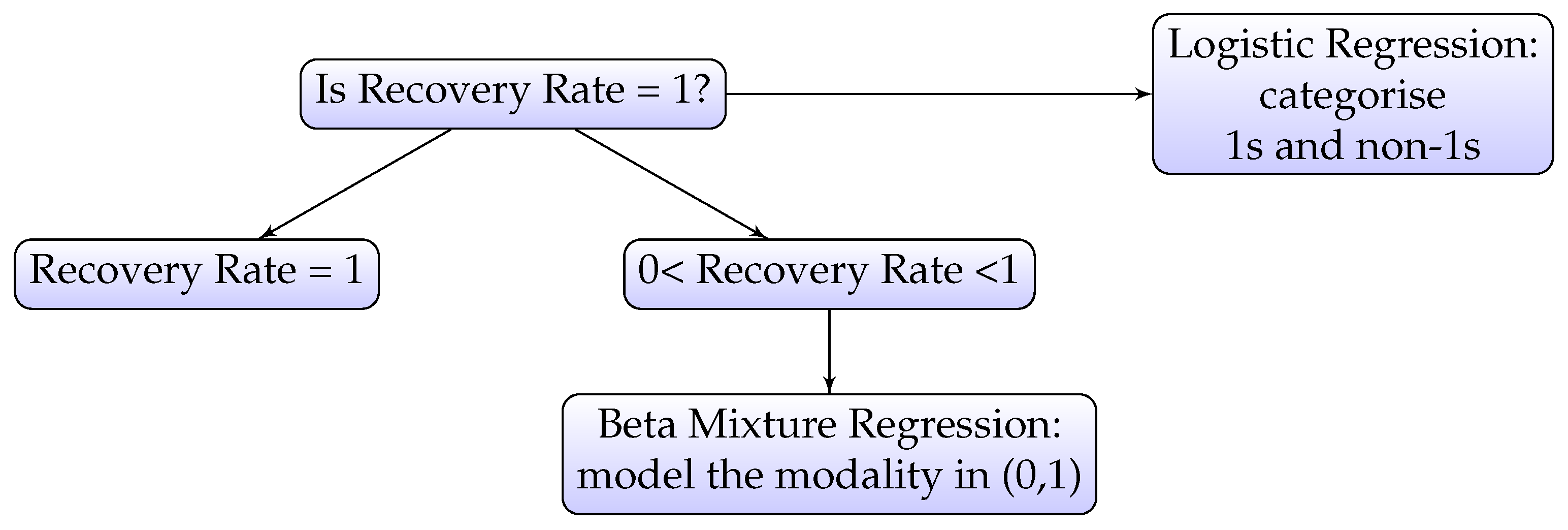
- A beta mixture model is parameterised by mean and precision based on two sets of predictor variables on the interval of (0, 1) in order to model the two modes located at just after 0 and around 0.55.
- A logistic regression model is used for the mode at boundary value 1.
2. Data
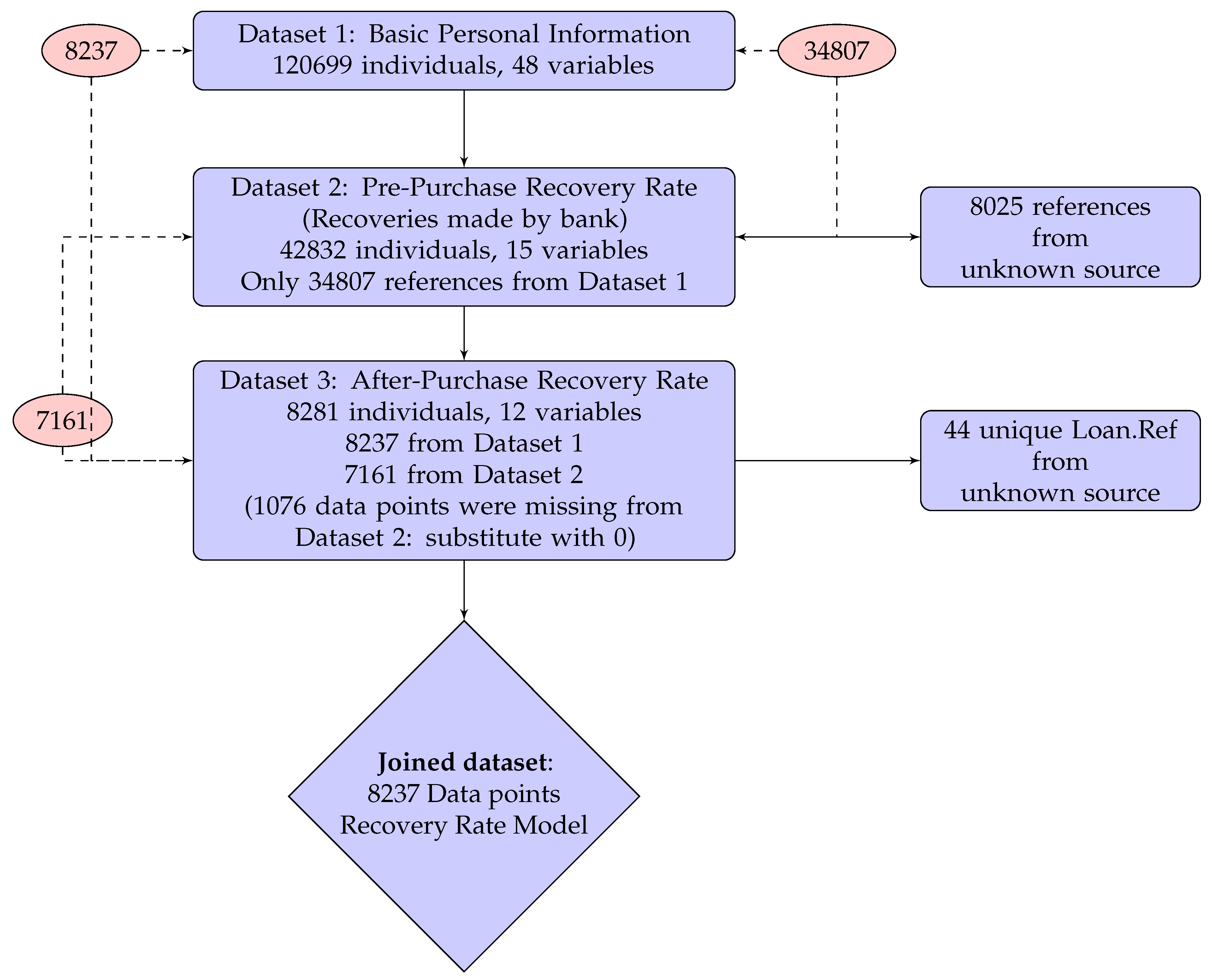
- Dataset 1
- provides 48 predictor variables of personal information including socio-demographic variables, Credit Bureau Score and debt status for 120,699 individuals for loans originating between January 1998 and May 2014 from several different financial institutions. Overall, 97.5% of them have credit card debt and only 2.5% are refinanced credit cards (product = “R”). Partial information was extracted from a Bad Debt Bureau. Each record corresponds to a bad loan and has a unique key Loan.Ref.
- Dataset 2
- records all the recoveries made by the bank before the debt collection company purchased the debt portfolio. It contains 15 predictor variables about historical collection information, which includes number of calls, contacts and visits made by the bank to collect the debt. It also includes repayments in the format of monthly summary. In total, there are 42,832 individuals’ records in Dataset 2, among which only 34,807 individuals can be matched to Dataset 1 by Loan.Ref. Numbers of calls, contacts, visits, repayment and some other monthly activities are aggregated by summing for each loan identified by Loan.Ref.
- Dataset 3
- records all the recoveries made by the debt collection company after they purchased the debt portfolio from the bank. It includes 12 predictor variables about the ongoing collection information. There are 8281 individuals in total, among which only 8237 individuals are from Dataset 1. Since only positive repayments are recorded, all the recovery rates we calculated are strictly greater than 0. Therefore, in the modelling section, we only focus on the recovery modelling in the interval (0, 1], which is slightly different from the usual RR defined in [0, 1]. The debt collection period recorded in this dataset is from January 2015 to end of November 2016.
Recovery Rate Calculation
3. Modelling Methodology
3.1. Linear Regression with Lasso
3.2. Multivariate Beta Regression
3.3. Inflated Beta Regression
3.4. Beta Mixture Model combined with Logistic Regression
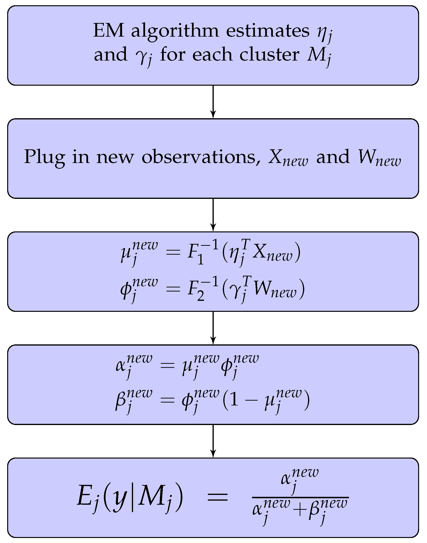
Predictions Using the Beta Mixture Model
- Assign the new observation to the cluster that achieves the highest log-likelihood. This is a hard clustering approach, which assigns the observation to exactly one cluster (Fraley and Raftery. 2002).
- Assign the new observation to each cluster j with probability . This is a soft clustering approach, which assigns the observation to a percentage weighted cluster (Leisch 2004).
4. Results
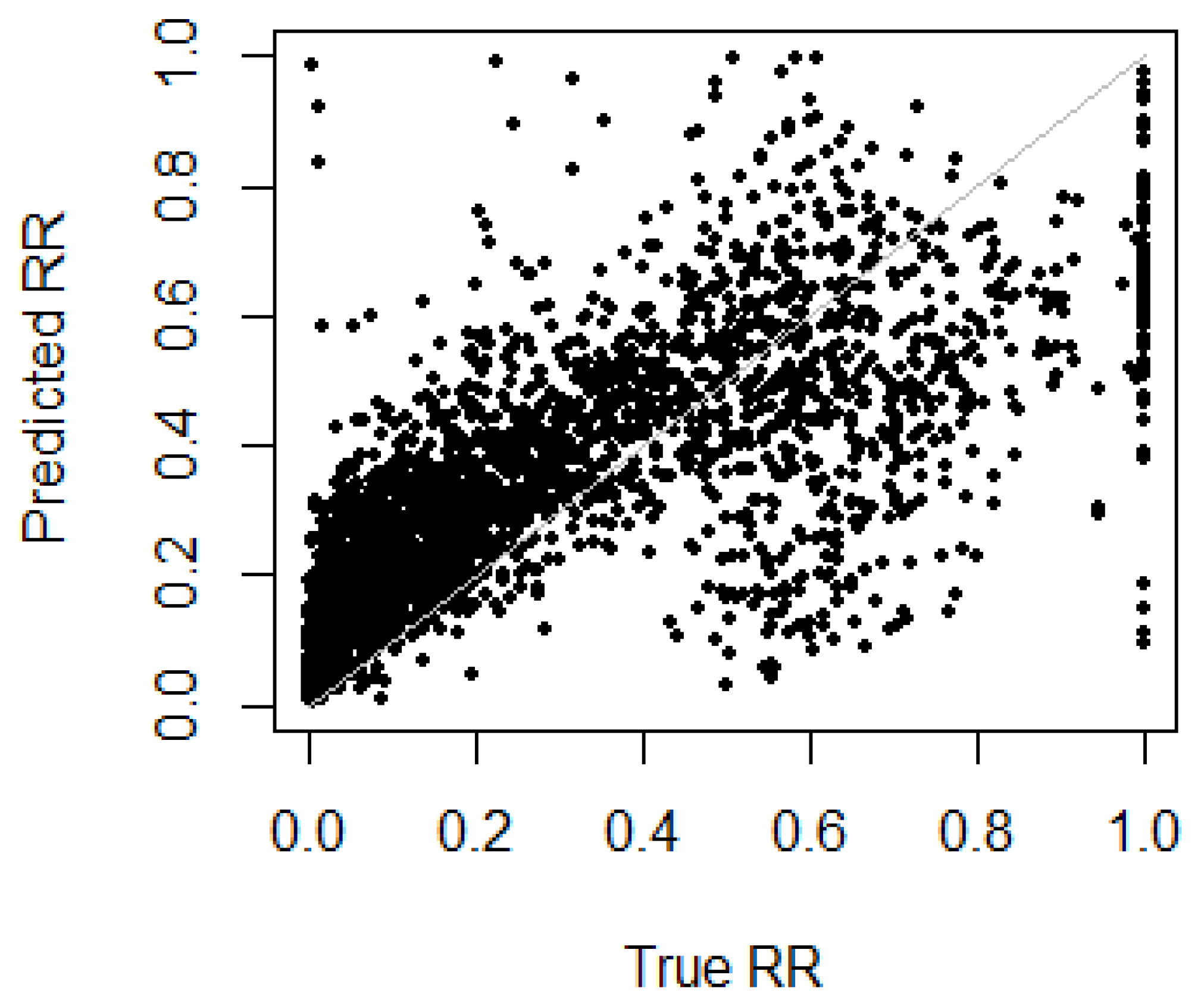
Model Performance
5. Conclusions
Author Contributions
Funding
Acknowledgments
Conflicts of Interest
Abbreviations
| IRB | Internal ratings based |
| RR | Recovery rate |
| LGD | Loss given default |
| PD | Probability of default |
| EAD | Exposure at default |
| EM | Expectation-Maximisation (algorithm) |
| MSE | Mean square error |
| MAE | Mean absolute error |
| MAAE | Mean absolute aggregate error |
Appendix A

| Variable | Type | Description | Statistics |
|---|---|---|---|
| RR post | numeric | Recovery rate (outcome variable) | 0.000508, 0.280 (0.283), 1 |
| Product | factor | Type of loan | C:7468 (90.7%), R:769 (9.3%) |
| Principal | numeric | Original loan amount | 0, 3120 (2330), 15000 |
| Interest | numeric | Interest payments | 0, 551 (439), 3380 |
| Insurance | numeric | Insurance fees | 0, 42 (84.6), 953 |
| Late charges | numeric | Late charge fees | 0, 269 (109), 1470 |
| Overlimit fees | numeric | Over credit limit fees | 0, 13.3 (24.6), 315 |
| Creditlimit | numeric | Credit limit | 0, 4560 (2660), 13800 |
| Sex | factor | Sex | F:3196 (38.8%), M:5041 (61.2%) |
| Married | factor | Marriage status | 0:1201 (14.6%), D:518 (6.3%), M:3929 (47.7%), O:217 (2.6%), S:2230 (27.1%), W:142 (1.7%) |
| Age | numeric | Age | 1, 48.7 (11.1), 87 |
| DelphiScore | integer | Credit bureau score | 0, 298 (138), 443 |
| Bureau Sub 1 | factor | Loan is in the servicer’s bureau (1 = True) | 0: 1520 (18.5%), 1: 6717 (81.5%) |
| CustPaymentFreq | integer | Customer repayment frequency | 1, 7.56 (5.59), 29 |
| Post Balance | numeric | Exposure amount at start of servicing | 0, 3130 (2630), 15900 |
| Total paid amount | numeric | Total net paid amount | −275, 1200 (1100), 11200 |
| Total calls | numeric | Total number of calls | 0, 104 (106), 911 |
| Total contacts | numeric | Total number of contacts (except calls) | 0, 28.5 (26.5), 196 |
| Bankreport Freq | numeric | Bank reporting frequency | 0, 11.6 (7.92), 26 |
| Pre recovery rate | numeric | Recovery rate | −0.130, 0.258 (0.217), 2.89 |
| Employer | factor | Employer known | EmployerProvided:8053 (97.8%), NoInfo:184 (2.2%) |
| Total number | integer | Total number of loan accounts | 0, 2.3 (2.43), 68 |
References
- Azzalini, Adelchi, and Giovanna Menardi. 2014. Clustering via nonparametric density estimation: The R package pdfCluster. Journal of Statistical Software 57: 1–26. [Google Scholar] [CrossRef]
- Bank for International Settlements. 2001. The Internal Ratings-based Approach. Basel: Bank for International Settlements. [Google Scholar]
- Bellotti, Tony, and Jonathan Crook. 2012. Loss given default models incorporating macroeconomic variables for credit cards. International Journal of Forecasting 28: 171–82. [Google Scholar] [CrossRef]
- Calabrese, Raffaella. 2012. Predicting bank loan recovery rates with a mixed continuous-discrete model. Applied Stochastic Models in Business and Industry 30: 99–114. [Google Scholar] [CrossRef]
- Cribari-Neto, Francisco, and Achim Zeileis. 2010. Beta regression in R. Journal of Statistical Software 34: 1–24. [Google Scholar] [CrossRef]
- Ferrari, Silvia, and Francisco Cribari-Neto. 2004. Beta regression for modelling rates and proportions. Journal of Applied Statistics 31: 799–815. [Google Scholar] [CrossRef]
- Fraley, Chris, and Adrian E Raftery. 2002. Model-based clustering, discriminant analysis, and density estimation. Journal of the American Statistical Association 97: 611–31. [Google Scholar] [CrossRef]
- Friedman, Jerome, Trevor Hastie, and Robert Tibshirani. 2010. Regularization paths for generalized linear models via coordinate descent. Journal of Statistical Software 33: 1–22. [Google Scholar] [CrossRef] [PubMed]
- Gruen, Bettina, Ioannis Kosmidis, and Achim Zeileis. 2012. Extended beta regression in R: Shaken, stirred, mixed, and partitioned. Journal of Statistical Software 48: 1–25. [Google Scholar] [CrossRef]
- Gruen, Bettina, and Friedrich Leisch. 2007. Fitting finite mixtures of generalized linear regressions in R. Computational Statistics & Data Analysis 51: 5247–52. [Google Scholar]
- Gruen, Bettina, and Friedrich Leisch. 2008. Flexmix version 2: Finite mixtures with concomitant variables and varying and constant parameters. Journal of Statistical Software 28: 1–35. [Google Scholar] [CrossRef]
- Hastie, Trevor, and Brad Efron. 2013. lars: Least Angle Regression, Lasso and Forward Stagewise, R package version 1.2; Available online: https://cran.r-project.org/web/packages/lars/lars.pdf (accessed on 18 February 2019).
- Ji, Yuan, Chunlei Wu, Ping Liu, Jing Wang, and Kevin R. Coombes. 2005. Applications of beta-mixture models in bioinformatics. Bioinformatics 21: 2118–22. [Google Scholar] [CrossRef] [PubMed]
- Laurila, Kirsti, Bodil Oster, Claus L. Andersen, Philippe Lamy, Torben Orntoft, Olli Yli-Harja, and Carsten Wiuf. 2011. A beta-mixture model for dimensionality reduction, sample classification and analysis. BMC Bioinformatics 12: 215. [Google Scholar] [CrossRef] [PubMed]
- Leisch, Friedrich. 2004. Flexmix: A general framework for finite mixture models and latent class regression in R. Journal of Statistical Software 11: 1–38. [Google Scholar] [CrossRef]
- Loterman, Gert, Iain Brown, David Martens, Christophe Mues, and Bart Baesens. 2012. Benchmarking regression algorithms for loss given default modeling. International Journal of Forecasting 28: 161–70. [Google Scholar] [CrossRef]
- Mittelhammer, Ron C., George Judge, and Douglas Miller. 2000. Econometric Foundations, 1st ed.Cambridge: Cambridge University Press. [Google Scholar]
- Moustafa, Nour, Gideon Creech, and Jill Slay. 2018. Anomaly Detection System using Beta Mixture Models and Outlier Detection. In Progress in Computing, Analytics and Networking. Advances in Intelligent Systems and Computing. Edited by Prasant Kumar Pattnaik, Siddharth Swarup Rautaray, Himansu Das and Janmenjoy Nayak. Singapore: Springer, vol. 710. [Google Scholar] [CrossRef]
- Nocedal, Jorge, and Stephen J. Wright. 1999. Numerical Optimization, 1st ed.Berlin: Springer. [Google Scholar]
- Papke, Leslie, and Jeffrey Wooldridge. Econometric methods for fractional response variables with an application to 401(k) plan participation rates. Journal of Applied Econometrics 11: 619–32. [CrossRef]
- Qi, Min, and Xinlei Zhao. 2011. Comparison of modeling methods for loss given default. Journal of Banking & Finance 35: 2842–55. [Google Scholar]
- Thomas, Lyn, and Katarzyna Bijak. 2015. Impact of Segmentation on the Performance Measures of LGD Models. Available online: https://crc.business-school.ed.ac.uk/wp-content/uploads/sites/55/2017/02/Impact-of-Segmentation-on-the-Performance-Measures-of-LGD-Models-Lyn-Thomas-and-Katarzyna-Bijak.pdf (accessed on 18 February 2019).


| Approach 2 | ||
|---|---|---|
| prior | Extract from the EM algorithm | Extract from the EM algorithm |
| Prior based on training set cluster size ratio | ||
| Indifferent Prior |
| Variables | Beta Mixture Model in (0, 1) | Beta Regression in (0, 1) | ||||
|---|---|---|---|---|---|---|
| M1 Estimate | Pr(>|z|) | M2 Estimate | Pr(>|z|) | Betareg Estimate | Pr(>|z|) | |
| (Intercept) | −0.67015 | <0.0001 | −2.62862 | <0.0001 | −1.80064 | <0.0001 |
| Product R | −0.03376 | 0.47711 | −0.00766 | 0.59733 | 0.02270 | 0.41766 |
| Principal | 0.00056 | NA | 0.00114 | NA | 0.00081 | 0.00000 |
| Interest | 0.00065 | <0.0001 | 0.00118 | NA | 0.00097 | 0.00000 |
| Insurance | 0.00082 | <0.0001 | 0.00116 | <0.0001 | 0.00086 | <0.0001 |
| Late Charges | 0.00042 | 0.00578 | 0.00115 | <0.0001 | 0.00072 | <0.0001 |
| Overlimit Fees | −0.00105 | 0.07594 | 0.00145 | <0.0001 | 0.00018 | 0.52533 |
| Credit limit | 0.00004 | NA | −0.00001 | NA | −0.00003 | <0.0001 |
| Sex = Male | 0.03659 | 0.17453 | −0.01412 | 0.13364 | 0.00969 | 0.43796 |
| Marital status = | ||||||
| Divorced | −0.01175 | 0.85305 | −0.01427 | 0.47359 | −0.03144 | 0.25840 |
| Married | −0.06356 | 0.10819 | −0.01476 | 0.16836 | −0.03850 | 0.01957 |
| Single | 0.00982 | 0.83178 | 0.00695 | 0.63324 | 0.00332 | 0.86926 |
| Widow | −0.14627 | 0.19497 | 0.02311 | 0.51404 | −0.03869 | 0.45314 |
| Other | 0.12328 | 0.17954 | −0.03476 | 0.22384 | 0.04570 | 0.24125 |
| Age | −0.00273 | 0.05378 | −0.00038 | 0.42389 | −0.00115 | 0.07159 |
| Credit Bureau Score | 0.00059 | 0.10337 | 0.00007 | 0.07890 | 0.00038 | 0.00222 |
| Bureau bad debt | −0.32990 | 0.01290 | -0.06936 | <0.0001 | −0.24123 | 0.00000 |
| Cust Payment Freq | 0.06530 | <0.0001 | 0.03506 | <0.0001 | 0.05046 | <0.0001 |
| Post Balance | −0.00106 | NA | −0.00127 | NA | −0.00103 | 0.00000 |
| Total Paid Amount | 0.00004 | NA | −0.00038 | NA | −0.00014 | <0.0001 |
| Total Calls | −0.00044 | 0.00515 | −0.00023 | 0.00275 | −0.00032 | <0.0001 |
| Total Contacts | −0.00136 | 0.03257 | 0.00040 | 0.08116 | −0.00031 | 0.28402 |
| Bank report Freq | −0.01719 | <0.0001 | −0.00407 | <0.0001 | −0.01117 | <0.0001 |
| Pre recovery Rate | 0.56850 | <0.0001 | 3.63447 | <0.0001 | 2.26212 | <0.0001 |
| EmployerNoInfo | −0.04457 | 0.63820 | −0.01277 | 0.65487 | 0.03439 | 0.38375 |
| Total Number | −0.00949 | 0.16151 | −0.00169 | 0.42951 | −0.00776 | 0.00651 |
| (Intercept) | 1.60514 | <0.0001 | 2.64737 | <0.0001 | 1.45450 | 0.00000 |
| Pre recovery Rate | 0.49096 | 0.00025 | −2.11510 | <0.0001 | −0.18488 | 0.01538 |
| Post Balance | 0.00039 | <0.0001 | 0.00018 | NA | 0.00031 | 0.00000 |
| Cust Payment Freq | 0.02949 | <0.0001 | 0.17612 | <0.0001 | 0.07759 | 0.00000 |
| Credit Bureau Score | −0.00058 | 0.00458 | −0.00033 | 0.09534 | −0.00028 | 0.01388 |
| Model | MSE | MAE | MAAE |
|---|---|---|---|
| Linear Regression | |||
| Linear regression | 0.024984 | 0.114268 | 0.025894 |
| Stepwise linear regression | 0.024752 | 0.113621 | 0.025700 |
| Linear regression with Lasso | 0.025228 | 0.114847 | 0.023739 |
| Linear regression, excluding Dataset 2 | 0.026822 | 0.121385 | 0.026303 |
| Beta regression | |||
| Standard beta regression | 0.085630 | 0.260459 | 0.161366 |
| Inflated beta regression | 0.076650 | 0.216374 | 0.048466 |
| Beta mixture model combined with logistic regression | |||
| Max log-likelihood | 0.018750 | 0.095432 | 0.030629 |
| Prior based on R Flexmix | 0.018460 | 0.091833 | 0.023991 |
| Prior based on training set cluster size ratio | 0.019325 | 0.092225 | 0.022594 |
| Indifferent Prior | 0.018030 | 0.092399 | 0.026298 |
© 2019 by the authors. Licensee MDPI, Basel, Switzerland. This article is an open access article distributed under the terms and conditions of the Creative Commons Attribution (CC BY) license (http://creativecommons.org/licenses/by/4.0/).
Share and Cite
Ye, H.; Bellotti, A. Modelling Recovery Rates for Non-Performing Loans. Risks 2019, 7, 19. https://doi.org/10.3390/risks7010019
Ye H, Bellotti A. Modelling Recovery Rates for Non-Performing Loans. Risks. 2019; 7(1):19. https://doi.org/10.3390/risks7010019
Chicago/Turabian StyleYe, Hui, and Anthony Bellotti. 2019. "Modelling Recovery Rates for Non-Performing Loans" Risks 7, no. 1: 19. https://doi.org/10.3390/risks7010019
APA StyleYe, H., & Bellotti, A. (2019). Modelling Recovery Rates for Non-Performing Loans. Risks, 7(1), 19. https://doi.org/10.3390/risks7010019