Article

On the Failure to Reach the Optimal Government Debt Ceiling

by
Abel Cadenillas
1,* and
Ricardo Huamán-Aguilar
2
1
Department of Mathematical and Statistical Sciences, University of Alberta, Central Academic Building 639, Edmonton, AB T6G 2G1, Canada
2
Department of Economics, Pontificia Universidad Católica del Perú, Av. Universitaria 1801, San Miguel, Lima 32, Peru
*
Author to whom correspondence should be addressed.
Risks 2018, 6(4), 138; https://doi.org/10.3390/risks6040138
Submission received: 19 September 2018 / Revised: 19 November 2018 / Accepted: 27 November 2018 / Published: 4 December 2018
(This article belongs to the Special Issue Applications of Stochastic Optimal Control to Economics and Finance)

Abstract

:
We develop a government debt management model to study the optimal debt ceiling when the ability of the government to generate primary surpluses to reduce the debt ratio is limited. We succeed in finding a solution for the optimal debt ceiling. We study the conditions under which a country is not able to reduce its debt ratio to reach its optimal debt ceiling, even in the long run. In addition, this model with bounded intervention is consistent with the fact that, in reality, countries that succeed in reducing their debt ratio do not do so immediately, but over some period of time. To the best of our knowledge, this is the first theoretical model on the debt ceiling that accounts for bounded interventions.

1. Introduction

1.1. Economic Motivations

The recent debt crisis in the world has proved that controlling the debt ratio of a country is of paramount importance. The literature on public debt management is abundant, from classical theoretical references such as Domar (1944); Barro (1989, 1999), and Dornbusch and Draghi (1990), to more applied ones such as Wheeler (2004); IMF (2002); IMF and World Bank (2001, 2003); Ghosh et al. (2013); Huamán-Aguilar and Cadenillas (2015); Woo and Kumar (2015) and Shah (2005). The theoretical literature deals with the optimal tax problem, and the effects of government debt. The applied references provide useful guidelines for practitioners.
There is also literature on debt sustainability. There are two interpretations of this term: the long-term meaning and the short-term meaning. The long-term meaning states that debt is sustainable if the total discounted path of governments expenses equals the total discounted path taxes. The medium term meaning defines that debt is sustainable if the debt-to-GDP ratio converges toward a target ratio over some period of time. Among theoretical references, we have, for example, Bohn (1995) and Blanchard et al. (2003). Among applied literature, we have, for instance, Balassone and Franco (2000) and Neck and Sturm (2008).
As Balassone and Franco (2000) point out, “the absence of a clear-cut theoretical benchmark to assess sustainability has often favoured the use of ad hoc definitions”. In 1992, the Maastricht Treaty selected 60 % as the upper bound for the debt-to-GDP ratio for countries to be members of the European Union1. In the USA, the nominal debt (measured in USA dollars, not debt-to-GDP ratio) has a ceiling that is determined by its Congress. However, the selection of the debt ceiling by politicians is not necessarily optimal. Indeed, Gersbach (2014) points out the following: “Politicians tend to push the amount of public debt beyond socially desirable levels in order to increase their reelection chances”.
Inspired by the preceding discussion, we define debt ceiling as the maximum level of debt ratio at which government intervention is not required. That is, if the debt ratio of a country is larger than its debt ceiling, the government should reduce the debt ratio by generating fiscal surpluses. Otherwise, the debt is said to be under control and there is no reason for interventions. This definition is consistent with the intended meaning given to the 60 % in the Maastricht Treaty (Article 104c). We remark that the government debt ceiling that we study in this paper is different from the following topics related to government debt management: optimal debt, credit ceiling, and debt limit2.
Uctum and Wickens (2000) study the debt sustainability for some countries considering the 60 % ceiling. In that research the debt ceiling is treated as exogenous. The literature in which the government debt ceiling is endogenous is scarce. As far as we know, the only mathematically rigorous research on the optimal government debt ceiling problem has been done by Cadenillas and Huamán-Aguilar (2016) and Ferrari (2018). In both papers, the government debt ceiling is endogenous. Cadenillas and Huamán-Aguilar (2016) study the optimal debt ceiling assuming that the interventions of a government to reduce its debt ratio are unbounded3. They succeed in finding an explicit formula for the optimal debt ceiling as a function of important macro-financial variables. Ferrari (2018) incorporates inflation in the model of Cadenillas and Huamán-Aguilar (2016) but does not present an explicit solution.
We consider a country whose government wants to impose an upper bound on its debt ratio. We assume that debt generates a disutility for the government of the country, which is an increasing and convex function of the debt ratio. On the other hand, the government can reduce its debt ratio, but there is a cost generated by this intervention. The government wants to minimize the expected total discounted cost (the cost of debt reduction plus the disutility of debt) taking into account that its ability to generate primary surpluses to reduce its debt ratio is limited. In such theoretical framework, we have found a solution for the optimal debt ceiling, which depends on key macro-financial variables, such as the interest rate on debt, the debt volatility, and the rate of economic growth. Moreover, we have obtained an optimal debt policy based on the optimal debt ceiling. It works in the following way. If the actual debt ratio of a country is below its optimal debt ceiling, then it is optimal for the government not to intervene. Otherwise, the government should intervene at the maximal rate to reduce its debt ratio. Given the constraint on the generation of primary surpluses, the controlled debt ratio may be sometimes or always above the optimal debt ceiling. Having in mind a country with debt problems, we also study the time to reach its debt ceiling (not necessarily its optimal debt ceiling) assuming that the current debt ratio is above its debt ceiling.

1.2. Contributions

We improve the results of Cadenillas and Huamán-Aguilar (2016) by studying the optimal debt ceiling when the government interventions to reduce its debt ratio have an upper bound. The motivation is that it is difficult for a country to obtain primary surpluses to reduce its debt ratio. The 60 % ceiling set in the Maastricht Treaty was part of the “convergence criteria”, in the understanding that countries whose debt ratio were above that threshold should reach the 60 % over a number of years. The model presented in this paper accounts for the important fact that countries in reality may or may not succeed in reaching their optimal debt ceilings. If they do, it takes some time to reach that goal. Our quantitative results differ from those of Cadenillas and Huamán-Aguilar (2016). For example, the optimal debt ceiling in our model is always smaller than the optimal debt ceiling in the unbounded case. Our qualitative results differ as well. Indeed, if the bound on government intervention is very large, then the debt ceiling is an increasing function of the volatility. That coincides with the unbounded case studied by Cadenillas and Huamán-Aguilar (2016). However, if the bound on government intervention is small, then the debt ceiling is a decreasing function of the volatility. That differs from the unbounded case studied by Cadenillas and Huamán-Aguilar (2016). We find that if the constraint to generate primary surpluses is severe (very low upper bound), a country may not be able to reach its optimal debt ceiling, even in the long run. For those countries which succeed in reaching their optimal debt ceiling, it may take some time to accomplish that goal. These findings are some of the main results of this research.
This paper is organized as follows: we present the model for bounded government debt management in Section 2. In Section 3, we present a verification theorem which states a sufficient condition for a debt control policy to be optimal. In Section 4, we find a candidate for solution and then verify that this candidate is indeed the solution. We study the time to reach a debt ceiling in Section 5. In Section 6 and Section 7, we perform an interesting economic analysis of the debt policy based on the government debt ceiling. We write the conclusions in Section 8.

2. The Bounded Government Intervention Model

We use a Brownian motion to model the uncertainty in the debt ratio. Formally, we consider a complete probability space ( Ω , F , P ) together with a filtration { F t } = { F t , t [ 0 , ) } , which is the P-augmentation of the filtration generated by a one-dimensional Brownian motion W.
We study the debt ratio X = { X t , t [ 0 , ) } of a country, which is defined by
X t : = gross public debt at time t gross domestic product ( GDP ) at time t .
This definition of the debt ratio is standard in the economics literature (see, for example, Uctum and Wickens (2000)).
Let r denote the interest rate on debt and g the rate of economic growth. Section 22.2 (p. 460) of Blanchard (2017), a standard reference on macroeconomics, states that
change of the debt ratio at time t = ( r g ) ( debt ratio at time t ) + primary deficit at time t gross domestic product ( GDP ) at time t .
He assumes a discrete-time deterministic model in which r and g are constants.
The continuous-time version of Blanchard (2017) can be written in integral form as
X t = x + 0 t ( r g ) X s d s 0 t u s d s ,
where x ( 0 , ) is the initial debt ratio, r [ 0 , ) is the interest rate on debt, g ( , + ) is the rate of economic growth, and u = u t , t [ 0 , ) is the rate of the primary balance (equivalently, the negative of the primary deficit).
Motivated by the uncertainty of the economy, we generalize the deterministic model (1) to the stochastic model
X t = x + 0 t ( r g ) X s d s + 0 t σ X s d W s 0 t u s d s .
The term 0 t σ X t d W s above accounts for the uncertainty in the economy, and models the empirical fact that the bigger the debt, the bigger the risk. Here, σ ( 0 , ) is the debt volatility.
The government intervenes to manage its debt ratio via the control process u = { u t , t [ 0 , ) } . This process represents the rate of intervention of the government, and it is associated with the generation of primary surpluses with the specific goal of reducing the debt ratio. Unlike Cadenillas and Huamán-Aguilar (2016), we assume that this control process is bounded. Indeed, for a fixed U ¯ > 0 , we assume that
u t [ 0 , U ¯ ] , t 0 ,
which means that the ability of the government to produce primary surpluses is limited, as it is in reality. We allow each country to have a different bound U ¯ , which depends on its structural economic and political characteristics.
The intervention of the government to reduce its debt ratio has a cost. This cost is generated by fiscal adjustments, which can take the form of reducing expenses or raising taxes. We denote the marginal cost of debt ratio reduction by k. That is, the government has to pay the cost k > 0 for each unit of debt ratio reduction. Let λ stand for the government discount rate. Thus, 0 e λ t k u t d t represents the cumulative discounted cost of reducing the debt ratio.
There are also costs for having debt. High public debt has negative effects on the economy. According to Blanchard (2017), high public debt means less growth of the capital stock and more tax distortions. Furthermore, it can make the fiscal policy extremely difficult. Moreover, Das et al. (2010) claim that it can generate a debt crisis, which, in turn, may lead to an economic crisis. On the other hand, having public debt may be beneficial for the economy, see, for example, Holmstrong and Tirole (1998). Since we are modelling a country that faces a debt problem, we disregard the positive effect of debt.
We assume that the government has a disutility function h : [ 0 , ) [ 0 , ) defined by
h ( y ) = α y m + 1 , where m { 1 , 2 , 3 , } .
Here, the parameter m represents the aversion of the government towards the debt ratio y. For example, countries which have never had a default (such as Canada and USA) have a lower parameter m than countries which have suffered debt crises (such as Argentina and Greece). The function h has the property of constant relative risk aversion (CRRA) equal to m (see Remark 1 below). We point out that this disutility function generalizes the quadratic function that is widely used in economics (see, for instance, Kydland and Prescott 1977, Taylor 1979, and Cadenillas and Zapatero 1999). On the other hand, the importance of debt for the government is represented by the parameter α , and it is measured in monetary units. The more important the debt, the larger the parameter α . The debt importance reflects the concern of the government to debt, and is usually determined in its economic plan.
Remark 1.
For a utility function u ( y ) , the risk aversion is defined to be y u ( y ) / u ( y ) (see, for instance, MasCollel et al. (1995) or Pratt (1964)). Similarly, for a disutility function h ( y ) , we define the relative risk aversion to be y h ( y ) / h ( y ) .
Thus, the expected total discounted cost (the cost of debt reduction plus the disutility of debt) is given by
J ( x ; u ) : = E x 0 e λ t h ( X t ) d t + 0 e λ t k u t d t .
Here, E x represents the conditional expected value given that X 0 = x .
Definition 1.
An adapted process u : [ 0 , ) × Ω [ 0 , U ¯ ] is called an admissible stochastic control if J ( x ; u ) < . The set of all admissible controls is denoted by A ( x ) .
Problem 1.
The government wants to select the control u A ( x ) that minimizes the functional J ( x ; · ) .
Thus, we can think of J as a loss function, a function that the government wants to minimize.
Proposition 1.
For every x ( 0 , ) , A ( x ) is a convex set and the function J ( x ; · ) is strictly convex. Furthermore, Problem 1 has at most one solution.
Proof. 
See Appendix A. □
We observe that for every u A ( x ) :
lim T E x e λ T X T m + 1 = 0 ,
because
0 e λ t E x α X t m + 1 d t = 0 e λ t E x h ( X t ) d t = E x 0 e λ t h ( X t ) d t < .
We will use condition (3) in the proof of Theorem 1 below. Condition (3) is a classical transversality condition.
We denote μ = r g . Since we want the nonintervention policy to be admissible (see details in Section 6.1), we assume the following condition on the discount rate:
λ > σ 2 m ( m + 1 ) / 2 + μ ( m + 1 ) .
This condition is consistent with the empirical observation that for governments the present is more important than the future. Condition (4) is similar to the ones imposed in economic models with infinite horizon (see, for instance, Romer 2002).

3. The Value Function and the Verification Theorem

The value function V : ( 0 , ) R is defined by
V ( x ) : = inf u A ( x ) J ( x ; u ) .
It measures the minimum loss for the government because it is the smallest cost that can be achieved when the initial debt ratio is x and we consider all the admissible controls.
Proposition 2.
The value function is nonnegative, increasing and convex. Furthermore, V ( 0 + ) = 0 , and it satisfies the polynomial growth condition
V ( x ) M x m + 1 ,
for some constant M ( 0 , ) .
Proof. 
See Appendix B. □
We state a sufficient condition for a policy to be optimal. First, we introduce the corresponding Hamilton–Jacobi–Bellman equation (HJB).
Let φ : ( 0 , ) R be a function in C 2 ( 0 , ) . The differential operator L is defined by
L u ( φ ( x ) ) : = 1 2 σ 2 x 2 φ ( x ) + μ x φ ( x ) u φ ( x ) λ φ ( x ) .
We consider the Hamilton-Jacobi-Bellman (HJB) equation
inf 0 u U ¯ L u ( v ( x ) ) + k u + h ( x ) = 0 ,
where v : ( 0 , ) R is a function in C 2 ( 0 , ) .
We next present a verification theorem that will be used to obtain the solution. Other verification theorems for classical stochastic control problems can be found, for instance, in Fleming and Soner (2006).
Theorem 1.
Let v C 2 ( ( 0 , ) ; [ 0 , ) ) be a convex function. If v satisfies the HJB Equation (7) and the polynomial growth condition
v ( x ) M x m + 1 ,
for some constant M > 0 , then for every u A ( x ) :
v ( x ) J ( x ; u ) .
Moreover, if the control u v , defined by
u v : = u v ( X t ) = a r g inf u [ 0 , U ¯ ] L u ( v ( X t ) ) + k u + h ( X t ) ,
is admissible, then
v ( x ) = J ( x ; u v ) .
That is, u ^ : = u v is the optimal control and V : = v is the value function for Problem 1.
Proof. 
Let u A ( x ) , and let X 0 = x > 0 . Since v is twice continuously differentiable, we may apply Ito’s formula to obtain for every s > 0 :
v ( x ) = e λ s v ( X s ) 0 s e λ t L u t v X t d t + 0 s e λ t v ( X t ) σ d W t ,
where L is defined in Equation (6). From the HJB Equation (7), we have L u t ( v ( X t ) ) + k u t + h ( X t ) 0 . Thus,
v ( x ) e λ s v ( X s ) + 0 s e λ t h ( X t ) d t + 0 s e λ t k u t d t + 0 s e λ t v ( X t ) σ d W t .
Let c R , such that x < c < . We define τ c : = inf { t 0 : X t = c } . We denote a b : = min ( a , b ) , where a and b are real numbers. Then, for every T 0 ,
v ( x ) e λ ( T τ c ) v ( X T τ c ) + 0 T τ c e λ t h ( X t ) d t + 0 T τ c e λ t k u t d t + 0 T τ c e λ t v ( X t ) σ d W t .
Taking conditional expectation given that X 0 = x , we obtain
v ( x ) E x e λ ( T τ c ) v ( X T τ c ) + E x 0 T τ c e λ t h ( X t ) d t + E x 0 T τ c e λ t k u t d t + E x 0 T τ c e λ t v ( X t ) σ d W t .
Since v C 2 ( ( 0 , ) ; [ 0 , ) ) and v is convex, we have v ( X t ) v ( c ) for every t [ 0 , T τ c ] . Thus,
E x 0 T τ c e λ t v ( X t ) σ 2 d t ( v ( c ) ) 2 σ 2 0 T e 2 λ t d t < .
Consequently, the stochastic integral
0 T τ c e λ t v ( X t ) σ d W t = 0 T e λ t v ( X t ) σ I { t [ 0 , τ c ] } d W t = : N T
is a square integrable martingale, and hence E x [ N T ] = N 0 = 0 . Here, I A is the indicator function of A.
Since v is a continuous function,
lim c e λ ( T τ c ) v ( X T τ c ) = e λ T v ( X T ) , P a . s .
Moreover, due to the polynomial growth condition (8), the family of random variables { e λ ( T τ c ) v ( X T τ c ) : c > x } is uniformly integrable (see Appendix D in Fleming and Soner 2006), and hence
lim c E x e λ ( T τ c ) v ( X T τ c ) = E x e λ T v ( X T ) .
The Monotone Convergence Theorem implies
lim c E x 0 T τ c e λ t h ( X t ) d t = E x 0 T e λ t h ( X t ) d t
and
lim c E x 0 T τ c e λ t k u t d t = E x 0 T e λ t k u t d t .
Taking the limit as c in (12),
v ( x ) E x e λ T v ( X T ) + E x 0 T e λ t h ( X t ) d t + E x 0 T e λ t k u t d t .
In view of (3), and the polynomial growth condition (8),
lim T E x e λ T v ( X T ) = 0 .
Taking the limit as T in (13), by the Monotone Convergence Theorem, we conclude
v ( x ) E x 0 e λ t h ( X t ) d t + 0 e λ t k u t d t = J ( x ; u ) .
This proves the first part of this theorem.
Next, we consider the second part of the theorem. Since u : = u v satisfies L u ( φ ( x ) ) + k u + h ( x ) = 0 , inequality (11) becomes an equality. Hence, the inequality in (14) becomes an equality for the admissible control u = u v . This completes the proof. □

4. The Solution

4.1. Construction of the Solution

Our goal in this subsection is to find a function that satisfies the conditions of Theorem 1. We note that the HJB Equation (7) can be expressed equivalently as
1 2 σ 2 x 2 v ( x ) + μ x v ( x ) λ v ( x ) + inf u [ 0 , U ¯ ] k v ( x ) u + h ( x ) = 0 .
Thus, we want to find a control that has the following form:
u ^ t : = arg inf u [ 0 , U ¯ ] k v ( X t ) u t = 0 , if v ( X t ) < k , U ¯ , if v ( X t ) k .
Consequently, to solve the HJB Equation (15) is equivalent to solve
1 2 σ 2 x 2 v ( x ) + μ x v ( x ) λ v ( x ) + h ( x ) = 0 ,
for v ( x ) < k ; and
1 2 σ 2 x 2 v ( x ) + μ x v ( x ) λ v ( x ) + k v ( x ) U ¯ + h ( x ) = 0 ,
for v ( x ) k .
Thus, a solution v of the HJB equation defines the regions C = C v and Σ = Σ v by
C : = x > 0 : 1 2 σ 2 x 2 v ( x ) + μ x v ( x ) λ v ( x ) + h ( x ) = 0 , v ( x ) < k ,
Σ : = x > 0 : 1 2 σ 2 x 2 v ( x ) + μ x v ( x ) λ v ( x ) + k v ( x ) U ¯ + h ( x ) = 0 , v ( x ) k .
We observe that the control u ^ takes the value zero on the region C , whereas it takes the value U ¯ on the region Σ . We conjecture that there exists a threshold b ( 0 , ) such that the government should intervene with u ^ = U ¯ when the debt ratio X b , and should not intervene (equivalently, u ^ = 0 ) when the debt ratio X < b . Accordingly, if v satisfies the HJB equation, we will call C = ( 0 , b ) the continuation region and Σ = [ b , ) the intervention region. Thus, it is natural to define the debt ratio ceiling as follows.
Definition 2.
Let v be a function that satisfies the HJB Equation (15), and C the corresponding continuation region. If C , the debt ratio ceiling b is
b : = sup { x ( 0 , ) | x C } .
Furthermore, if v is equal to the value function, then b is said to be the optimal debt ceiling.
Hence, we need to find the value function to obtain the optimal debt ceiling. The general solution of the HJB equation depends on whether we consider the continuation region C or the intervention region Σ . We have applied the power series method to obtain the solution on the region Σ .
To simplify the notation, we consider the power series
H y p e r g e o m e t r i c 1 F 1 ( θ ; η ; z ) : = 1 + n = 1 ( θ ) n ( η ) n 1 n ! z n , K ( θ ; η ; x ) : = 1 + n = 1 ( θ ) n ( η ) n 1 n ! 2 U ¯ σ 2 x n .
Here, θ ( , ) and η ( , ) are constants, and we denote
( a ) n : = Π j = 0 n 1 ( a + j ) = a ( a + 1 ) ( a + 2 ) ( a + n 1 ) , a R , n N .
This function H y p e r g e o m e t r i c 1 F 1 ( θ ; η ; z ) belongs to the family of hypergeometric functions. For a reference of these functions, and their relationship to second order differential equations, see, for example, Bell (2004) and Kristensson (2010).
Thus, the solution of the HJB equation is given by
v ( x ) = A 1 x γ 1 + A 2 x γ 2 + α ξ x m + 1 , if x C = ( 0 , b ) , f ( x ) , if x Σ = [ b , ) ,
with
f ( x ) = j = 0 m + 1 ζ j x j + B 1 x γ 2 σ 2 2 U ¯ γ 2 1 + n = 1 ( γ 2 ) n ( c 2 ) n 1 n ! 2 U ¯ σ 2 x n + B 2 2 U ¯ σ 2 x c 3 1 + n = 1 ( c 3 ) n ( 2 c 2 ) n 1 n ! 2 U ¯ σ 2 x n = j = 0 m + 1 ζ j x j + B 1 x γ 2 σ 2 2 U ¯ γ 2 K γ 2 , c 2 , x + B 2 2 U ¯ σ 2 x c 3 K c 3 , 2 c 2 , x ,
where A 1 , A 2 , B 1 and B 2 are some constants to be found. Furthermore, we define
μ ˜ : = μ 1 2 σ 2 ,
γ 1 : = μ ˜ μ ˜ 2 + 2 λ σ 2 σ 2 < 0 ,
γ 2 : = μ ˜ + μ ˜ 2 + 2 λ σ 2 σ 2 > 0 ,
ξ : = 1 λ σ 2 m ( m + 1 ) / 2 μ ( m + 1 ) > 0 ,
c 2 : = 2 1 γ 2 μ σ 2 ,
c 3 : = γ 2 + 2 μ ˜ σ 2 ,
ζ j : = m + 1 j α ( m + 1 j ) ! U ¯ m + 1 j i = j m + 1 i μ + i ( i 1 ) σ 2 / 2 λ , j { 2 , 3 , , m + 1 } ,
ζ 1 : = 2 U ¯ μ λ ζ 2 ,
ζ 0 : = k U ¯ λ U ¯ λ ζ 1 .
Remark 2.
By definition (21), one can verify that
lim x K γ 2 , c 2 , x = 1 , lim x K c 3 , 2 c 2 , x = 1 .
To guarantee the existence of the parameters { ζ j : j = 2 , 3 , , m + 1 } defined in (29), in addition to condition (4), we need to assume
λ j ( j 1 ) σ 2 2 + j μ , j { 2 , 3 , , m } .
We observe that, in the special case μ 0 , the inequality (4) implies (32).
Lemma 1.
The parameters of the model satisfy the following conditions:
(i) 
ξ > 0 ,
(ii) 
λ > μ ,
(iii) 
γ 2 > m + 1 ,
(iv) 
c 3 > 0 .
Proof. 
Part ( i ) follows immediately from (4). Part ( i v ) follows directly from the definition of γ 2 . Let us show ( i i ) . If μ > 0 , then condition (4) implies that λ > μ . If μ 0 , then λ > 0 μ .
To prove ( i i i ) , we define
f ˜ ( y ) = μ ˜ 2 + 2 y σ 2 σ 2 μ ˜ σ 2 ,
where μ ˜ = μ 0.5 σ 2 . We note that f ˜ is strictly increasing. By definition, γ 2 = f ˜ ( λ ) . If μ ˜ + σ 2 ( m + 1 ) 0 , then γ 2 = f ˜ ( λ ) > f ˜ ( m + 1 ) 2 σ 2 / 2 + μ ˜ ( m + 1 ) = m + 1 , where the inequality follows from (4). If μ ˜ + σ 2 ( m + 1 ) < 0 , then γ 2 = f ˜ ( λ ) > f ˜ ( 0 ) > 2 ( m + 1 ) , since λ > 0 . □
We recall that Proposition 2 implies V ( 0 + ) = 0 , and that the value function V satisfies the polynomial growth condition (5). Furthermore, we conjecture that v is twice continuously differentiable. Then, the five constants A 1 , A 2 , B 1 , B 2 and b can be found from the following five conditions:
v ( 0 + ) = 0 ,
v ( x ) M x m + 1 ,
v ( b + ) = v ( b ) ,
v ( b + ) = v ( b ) .
From Equations (19) and (20), we see that Equation (37) is equivalent to v ( b ) = k , which in turn is equivalent to
A 2 γ 2 b γ 2 1 + ( m + 1 ) α ξ b m = k .
Since γ 1 < 0 , condition (34) implies A 1 = 0 in the equation for v. Moreover, in the lemma below, we show that B 1 = 0 .
Lemma 2.
Suppose f, defined in (22), is non-negative and satisfies the polynomial growth condition
f ( x ) M x m + 1 ,
for some M > 0 . Then, B 1 = 0 .
Proof. 
See Appendix C. □
Hence, the candidate for value function is defined by
v ( x ) = A 2 x γ 2 + α ξ x m + 1 , if x C = ( 0 , b ) , f 1 ( x ) , if x Σ = [ b , ) ,
with
f 1 ( x ) : = j = 0 m + 1 ζ j x j + B 2 2 U ¯ σ 2 x c 3 K c 3 , 2 c 2 , x ,
where the remaining three constants A 2 , B 2 and b are found by solving the system of nonlinear Equations (36)–(38).
In summary, our candidate for value function is given by (40), and our candidate for optimal control is given by u ^ t : = 0 , if X t < b , U ¯ , if X t b . Moreover, our candidate for optimal debt ceiling is b. Naturally, we expect b to depend on the underlying parameters of the model ( μ , σ , λ , k , α , m , U ¯ ) , where μ = r g .
Now, we describe a procedure to solve the system (36)–(38). Noting that
K ( θ ; η ; x ) = n = 1 ( θ ) n ( η ) n 1 ( n 1 ) ! σ 2 2 U ¯ 2 U ¯ σ 2 x n + 1 , K ( θ ; η ; x ) = n = 1 ( θ ) n ( η ) n ( n + 1 ) ( n 1 ) ! σ 2 2 U ¯ 2 2 U ¯ σ 2 x n + 2 ,
we have
f 1 ( x ) = j = 0 m ( j + 1 ) ζ j + 1 x j B 2 c 3 2 U ¯ σ 2 x c 3 + 1 K ( c 3 ; 2 c 2 ; x ) + B 2 2 U ¯ σ 2 x c 3 K ( c 3 ; 2 c 2 ; x ) ,
f 1 ( x ) = j = 0 m 1 ( j + 2 ) ( j + 1 ) ζ j + 2 x j + B 2 c 3 ( c 3 + 1 ) 2 U ¯ σ 2 x c 3 1 x 2 K ( c 3 ; 2 c 2 ; x ) B 2 c 3 σ 2 2 U ¯ + σ 2 ( 2 U ¯ ) 2 2 U ¯ σ 2 x c 3 + 1 K ( c 3 ; 2 c 2 ; x ) + B 2 2 U ¯ σ 2 x c 3 K ( c 3 ; 2 c 2 ; x ) = j = 0 m 1 ( j + 2 ) ( j + 1 ) ζ j + 2 x j + B 2 c 3 ( c 3 + 1 ) 2 U ¯ σ 2 x c 3 1 x 2 K ( c 3 ; 2 c 2 ; x ) c 3 σ 2 2 U ¯ + σ 2 ( 2 U ¯ ) 2 2 U ¯ σ 2 x c 3 + 1 K ( c 3 ; 2 c 2 ; x ) + 2 U ¯ σ 2 x c 3 K ( c 3 ; 2 c 2 ; x ) .
To simplify the notation, consider the functions R and S defined by
R ( x ) : = 2 U ¯ σ 2 x c 3 K ( c 3 ; 2 c 2 ; x ) , S ( x ) : = c 3 ( c 3 + 1 ) 2 U ¯ σ 2 x c 3 1 x 2 K ( c 3 ; 2 c 2 ; x ) c 3 σ 2 2 U ¯ + σ 2 ( 2 U ¯ ) 2 2 U ¯ σ 2 x c 3 + 1 K ( c 3 ; 2 c 2 ; x ) + 2 U ¯ σ 2 x c 3 K ( c 3 ; 2 c 2 ; x ) .
Then, Equation (36) can be rewritten as
A 2 b γ 2 + α ξ b m + 1 = j = 0 m + 1 ζ j b j + B 2 R ( b )
and Equation (38) can be rewritten as
A 2 γ 2 ( γ 2 1 ) b γ 2 2 + α ξ ( m + 1 ) m b m 1 = j = 0 m 1 ( j + 2 ) ( j + 1 ) ζ j + 2 x j + B 2 S ( b ) .
Thus, Equations (36) and (38) are equivalent to
A 2 = A 2 ( b ) = ( j = 0 m + 1 ζ j b j α ξ b m + 1 ) S ( b ) + ( α ξ ( m + 1 ) m b m 1 j = 0 m 1 ( j + 2 ) ( j + 1 ) ζ j + 2 b j ) R ( b ) b γ 2 S ( b ) γ 2 ( γ 2 1 ) b γ 2 2 R ( b ) ,
B 2 = B 2 ( b ) = A 2 ( b ) b γ 2 + α ξ b m + 1 j = 0 m + 1 ζ j b j R ( b ) .
Then, Equation (37), or equivalently Equation (39), can be rewritten as
A 2 ( b ) γ 2 b γ 2 1 + ( m + 1 ) α ξ b m = k .
Let us consider the function w : ( 0 , ) ( , ) defined by
w ( y ) : = A 2 ( y ) γ 2 y γ 2 1 + ( m + 1 ) α ξ y m .
The procedure to solve Equations (36)–(38) is first to solve equation
w ( b ) = k ,
and then obtain A 2 and B 2 from Equations (42) and (43), respectively.

4.2. Verification of the Solution

In this subsection, we will prove rigorously that our candidate for optimal control is indeed the optimal control, and our candidate for value function is indeed the value function.
Theorem 2.
Let b be solution of Equation (44), and A 2 and B 2 be constants determined by (42) and (43). Let us define the function V : ( 0 , ) [ 0 , ) by
V ( x ) = v ( x ) = A 2 x γ 2 + α ξ x m + 1 , i f x ( 0 , b ) , f 1 ( x ) , i f x [ b , ) ,
with f 1 defined by Equation (41). Furthermore, let us define the process u ^ by
u ^ t : = U ¯ I { X ^ t b } ( t ) = 0 , i f X ^ ( t ) < b , U ¯ , i f X ^ ( t ) b .
If
x ( 0 , ) : V ( x ) > 0 ,
then V is the value function, b is the optimal debt ceiling, and u ^ is the debt policy generated by the optimal debt ceiling. Here, I A is the indicator function of A.
Proof. 
It is sufficient to show that all the conditions of Theorem 1 are satisfied. We observe that V ( 0 + ) = 0 . By construction, we get immediately that V C 2 ( 0 , ) . In view of (47), V is strictly convex. Thus, V ( x ) is strictly increasing. Next, we will show that V ( 0 + ) = 0 . We note that for every x ( 0 , b ) :
V ( x ) = x m ( m + 1 ) α ξ + A 2 γ 2 x γ 2 m 1 .
We recall that γ 2 > m + 1 by Lemma 1. Thus, V ( 0 + ) = 0 . Consequently, V ( x ) > 0 for every x > 0 . Hence, V is strictly increasing.
Next, we will show that V satisfies the HJB Equation (7). We recall that condition (39) is equivalent to V ( b ) = k . Since V ( x ) > 0 for every x ( 0 , ) , we conclude 0 < V ( x ) < k for every x ( 0 , b ) , and V ( x ) > k for every x ( b , ) . By construction, V satisfies (17) on ( 0 , b ) , and (18) on ( b , ) . Hence, V satisfies the HJB equation for all x ( 0 , ) . This also shows that indeed C = ( 0 , b ) and Σ = [ b , ) . Regarding the value function, it remains to verify that V satisfies the polynomial growth condition (8). Since
lim x K c 3 , 2 c 2 , x = 1
by Remark 2, and c 3 > 0 by Lemma 1, we obtain
lim x B 2 2 U ¯ σ 2 x c 3 K c 3 , 2 c 2 , x = 0 .
This implies that V is bounded above by a polynomial of degree m + 1 on the interval [ b , ) . On the other hand, on the interval ( 0 , b ) , the function V is bounded above by | A 2 | b γ 2 + α ξ b m + 1 . Hence, V satisfies the polynomial growth condition (8). Consequently, by Theorem 1, V is the value function. Since
J ( x ; u ^ ) J ( x ; 0 ) + E x 0 e λ t U ¯ d t = α ξ x m + 1 + U ¯ 1 λ < ,
by Section 6.1, we conclude that u ^ is admissible. Therefore, u ^ is the optimal debt policy. By Definition 2, the constant b is the optimal debt ceiling. This completes the proof of this theorem. □

4.3. The Debt Policy Generated by the Optimal Debt Ceiling

We observe that under the debt policy (46) generated by the optimal debt ceiling, the optimal debt ratio is given by
X ^ t = x + 0 t ( r g ) X ^ s d s + 0 t σ X ^ s d W s 0 t U ¯ I { X ^ s b } d s .
When the actual debt ratio X ^ t is below the optimal debt ceiling b, the definition of debt control given in Equation (46) states that u ^ ( t ) = 0 . Hence, the government does not generate primary surpluses to reduce its debt ratio. When the debt ratio reaches b and tries to cross it, the optimal control states that u ^ t = U ¯ . In other words, the government intervenes to reduce the debt ratio with the maximal rate U ¯ allowed. When the actual debt ratio X ^ t is strictly greater than the optimal debt ceiling b, the optimal debt policy in the bounded model states that the government reduces its debt ratio with the maximal rate U ¯ .
Suppose that the actual debt ratio is below the optimal debt ceiling b. Then, the government might or might not succeed in preventing the debt ratio from crossing b, the result depends on the values of the underlying parameters of the model, in particular on U ¯ . Specifically, the higher the parameter U ¯ , the more likely the controlled debt ratio will remain below the optimal debt ceiling b (see Section 5). This result differs from the unbounded case of Cadenillas and Huamán-Aguilar (2016) in which the optimal policy states that once the actual debt ratio is below or equal to its debt ceiling, it will remain there all the time.
On the other hand, if the current debt ratio is strictly greater than the optimal debt ceiling b, the optimal debt policy states that the government should reduce the debt ratio with the maximal rate U ¯ . Certainly, there is no guarantee that the resulting debt ratio will equal the debt ceiling b immediately because it may take some time to accomplish that goal, if that ever happens. Indeed, in Section 5, we present Example 2 in which the expected time to reach the optimal debt ceiling is strictly positive. Furthermore, if the government constraint is too severe (very low U ¯ ), there is a high probability that the country will never reach its optimal debt ceiling (see Example 3 in Section 5). In contrast, in the unbounded model of Cadenillas and Huamán-Aguilar (2016), the optimal debt ceiling is reached immediately.

4.4. Numerical Solutions

The solution of the problem involves the numerical solution of the system of three Equations (36)–(38) with three unknowns: A 2 , B 2 and b. We have written a program in Mathematica 11.0 to solve numerically those equations (see Appendix E). We get immediate solutions in a standard personal computer. We now present an example to illustrate the solution.
Example 1.
Let us consider the parameter values
r = 0.10 , g = 0.05 , σ = 0.05 , λ = 0.7 , k = 1 , U ¯ = 0.05 , m = 3 , α = 1 .
Solving numerically the Equation (44), we obtain b = 54.2756 % . Alternatively, we can solve numerically the system of Equations (36)–(38).
The graph of the corresponding value function is shown in Figure 1. We observe that condition (47) is satisfied. Thus, the value function is increasing, strictly convex, and twice continuously differentiable.
The optimal debt ratio ceiling is 54.2756 % . Thus, the corresponding debt policy is given by
u ^ t = 0 , if X t < 54.2756 % , 0.05 , if X t 54.2756 % .
That is, if the actual debt ratio is below the level 54.2756 % , the government should not intervene. Otherwise, the government should intervene with the maximal allowed rate of 0.05 . Given such constraint, there is no guarantee that the resulting debt ratio after intervention of the government will remain below 54.2756 % ; it may be the case that sometimes the debt ratio is above that threshold.
Remark 3.
We conjecture that condition (47) in Theorem 2 is satisfied for every solution of the system of Equations (36)–(38). This is actually the case in all the numerical examples that we have studied to calculate the optimal debt ceiling (see Section 4.4, Section 5.4, Section 6.2 and Section 6.3).

5. Time to Reach the Debt Ceiling

We study the time to reach a debt ceiling c considering that the government follows the debt policy u ( c ) defined by
u t ( c ) : = 0 , if X t < c , U ¯ , if X t c .
We define the stopping time
τ : = inf t > 0 : X ( t ) = c .
In this section, c > 0 is a constant real number that represents a ceiling for the debt ratio. We emphasize that c is any debt ceiling, not necessarily the optimal debt ceiling found in the previous section. In particular, c could be equal to the ceiling 60 % imposed by the Maastricht Treaty for the European Union.

5.1. The Theoretical Result

In general, the current or initial debt ratio of a country X 0 = x could be below or above the debt ceiling c. If a country selects c as its debt ceiling, and follows the debt policy u ( c ) , the dynamics of the debt ratio (2) becomes
X t ( c ) = x exp ( r g 0.5 σ 2 ) t + σ W t , if x < c , t τ , x exp ( r g 0.5 σ 2 ) t + σ W t U ¯ 0 t V t V u d u , if x > c , t τ ,
where
V t : = exp ( r g 0.5 σ 2 ) t + σ W t .
We can study the time τ to reach the debt ceiling for both cases, i.e., x < c or x > c . However, given the debt problems that motivate this research, it is compelling to study the time to reach the debt ceiling assuming x > c .
We recall that μ ˜ : = r g 1 2 σ 2 . We need to distinguish two cases: μ ˜ 0 and μ ˜ > 0 .
Proposition 3.
Suppose x > c . The following assertions are valid:
(i) 
If μ ˜ 0 or, equivalently, r g σ 2 / 2 , then
P x τ < = 1 .
(ii) 
If μ ˜ > 0 or, equivalently, r g > σ 2 / 2 , then
P x τ < = Γ ( ν 1 ) Γ ( ν 1 , β / x ) Γ ( ν 1 ) Γ ( ν 1 , β / c ) ,
where ν = 2 μ / σ 2 and β = 2 U ¯ / σ 2 , Γ ( · ) is the Gamma function, and Γ ( · , · ) is the incomplete Gamma function defined by
Γ ( a , z ) : = z t ( a 1 ) e t d t , z 0 , a > 0 .
Furthermore,
lim U ¯ P x { τ < } = 1 .
Proof. 
See Appendix D. □
Proposition 3 provides different conclusions depending on the parameters of the economy. Part (i) is associated with countries that have a big economic growth, and Part (ii) with countries with moderate economic growth.

5.2. Application 1: Countries with Big Economic Growth

If
g + σ 2 / 2 r ,
Part (i) of Proposition 3 states that the debt ceiling is reached with probability one, regardless of the level U ¯ of maximal rate. In other words, if the interest rate is lower that the rate of economic growth, plus an adjustment by volatility, then the debt ratio tends to decrease until it reaches the debt ceiling with probability one. The intuition behind the result is that the economic growth is big enough to control the debt ratio. This is a consequence of the definition of debt ratio, namely, debt ratio = debt in nominal currency / gross domestic product . Consequently, economies in which the rate of economic growth satisfy the above condition will be successful in reaching the debt ceiling.
For economies that satisfy the above condition (55), we can compute the expected time to reach the debt ceiling c. We illustrate this point in the following example.
Example 2.
We consider a country with parameter values
r = 0.05 , g = 0.10 , σ = 0.05 , U ¯ = 0.01 ,
and initial debt ratio x = 100 % . Suppose that this country selects c = 80 % as its debt ceiling.
For the above parameters, the expected time to reach the debt ceiling is E [ τ ] = 3.58 , with a 95 % confidence interval given by [ 3.5540 , 3.6136 ] . We have performed Monte Carlo simulations with 10 , 000 sample paths and time steps equal to 0.001 . That is, it takes 3.58 years on average to reach the debt ceiling 80 % , starting at the initial debt ratio of 100 % , and assuming that the government can decrease the debt ratio at the maximal rate. For a reference on Monte Carlo simulations see, for instance, Brandimarte (2002).

5.3. Application 2: Countries with Moderate Economic Growth

Now consider Part (ii) of Proposition 3. It refers to countries that have moderate economic growth in the sense that they satisfy the condition μ ˜ > 0 , which is equivalent to
g + σ 2 / 2 < r .
The probability to reach the optimal debt ceiling is given by the formula (53) that depends on ( r , g , σ , U ¯ , c ) . To illustrate the role played by the parameter U ¯ , we present a numerical example.
Example 3.
To study the role played by U ¯ on the probability of reaching c, we set c = 60 % , which is the ceiling proposed by the Maastricht Treaty for the European Union. We consider the set of parameter values
r = 0.10 , g = 0.05 , σ = 0.05 .
We consider two countries: Country A with initial debt ratio of 70 % (approximately the current debt ratio of Germany) and Country B with initial debt ratio of 170 % (approximately the current debt ratio of Greece). For simplicity, we assume that the other parameters values are the same for both countries.
In Table 1, we observe that, regardless of the type of country, there exist levels of the maximal rate of intervention U ¯ for which a country has very low probability of reaching the debt ceiling. For instance, if U ¯ = 2.5 % , then Country B has zero probability of reaching the debt ceiling, while Country A has only around 20 % of probability of reaching it. That is, severe constraints to generate primary surpluses lead to a high probability of never reaching the debt ceiling. Even worse, countries with severe constraints and high initial debt ratios, such as Country B, have probabilities close to zero of ever reaching their debt ceilings.
In addition, in Table 1, we observe that, as expected, the higher the maximal rate of intervention U ¯ , the greater the probability of reaching the debt ceiling, regardless of the type of country. In addition, there is a finite level of U ¯ such that the probability of reaching the optimal debt ceiling is one. For Country B, such level is U ¯ = 0.15 and for Country A it is around U ¯ = 0.05 .

5.4. Application 3: Time to Reach the Optimal Debt Ceiling

Now, we study the time to reach the optimal debt ceiling b for countries with moderate economic growth. That is, we consider the setting of Part (ii) of Proposition 3, taking c = b . To compute the optimal debt ceiling, we consider the parameters ( r , g , σ ) given in Example 3, and in addition the following parameter values:
λ = 0.7 , k = 1 , m = 1 , α = 0.5 .
As in the previous subsection, we consider Country A with initial debt ratio 70 % , and Country B with initial debt ratio 170 % .
In Table 2, we present the optimal debt ceiling that corresponds to the parameters given above, and the value of U ¯ given in the first column of that table. Then, for each set of parameters ( r , g , σ , U ¯ , b ) , we perform the calculations of the probability of reaching the optimal debt ceiling using Formula (53), with c = b . The probabilities of reaching the optimal debt ceiling b for Country A and Country B are presented in columns 3 and 4, respectively.
We note that the conclusions from Table 2 are the same as those from Table 1, namely, severe constraints on U ¯ imply that a country may not be able to reach its optimal debt ceiling, and the probability of eventually reaching its optimal debt ceiling increases with the value of U ¯ .
For a country with no severe constraint, that is able to reach its optimal debt ceiling, we have computed the expected time to reach its optimal debt ceiling by Monte Carlo simulations. For instance, for Country A with U ¯ = 0.1 , the expected time of reaching its debt ceiling is 0.6877 , while for Country B, with U ¯ = 0.15 , such value is 11.98 .
To sum up, we conclude that countries with severe constraints to generate primary surpluses (very low U ¯ ) have zero or very low probability of ever reaching their debt ceilings. This is one of the main results of this research, and represents a dramatic difference with the work of Cadenillas and Huamán-Aguilar (2016), in which the corresponding optimal debt ceiling is reached immediately with probability one.

6. Comparative Statics Analysis

In this section, we consider different parameter values in order to analyze the debt policy associated with the optimal debt ceiling. Specifically, we are going to make the following three analyses:
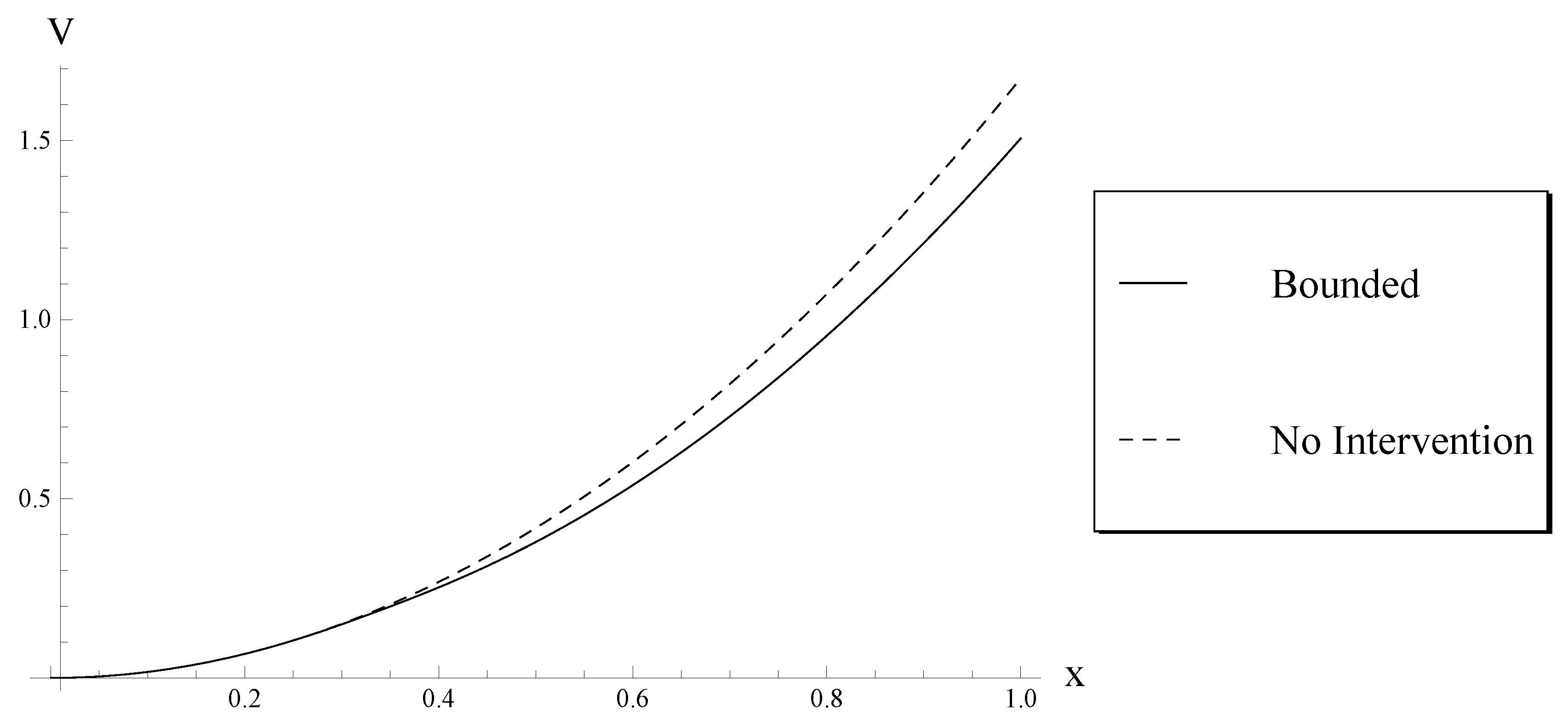
  • Compare the results of the debt policy associated with the optimal debt ceiling with the policy of non-government intervention.
  • Compare the results of the debt policy associated with the optimal debt ceiling presented in this paper with the policy derived in the unbounded model of Cadenillas and Huamán-Aguilar (2016).
  • Analyze the effects of some parameters on the optimal debt ceiling.
Unless otherwise stated, the basic parameter values that we will use in this section are given in the following example.
Example 4.
Let us consider the basic parameter values:
μ = 0.05 , σ = 0.05 , λ = 0.7 , k = 1 , U ¯ = 0.01 , m = 1 , α = 1 .
Solving numerically Equations (36)–(38), we obtain b = 31.04266 % .
We remark that, as Examples 1 and 4 show, the 60 % proposed by the Maastricht Treaty is not necessarily an optimal debt ceiling. In contrast to the 60 % proposed by the Maastricht Treaty, the optimal debt ceiling proposed in our paper depends on the specific characteristics of the country, which are reflected in the parameters’ values. We recall that that 60 % was simply the median of the debt ratio of some European countries.

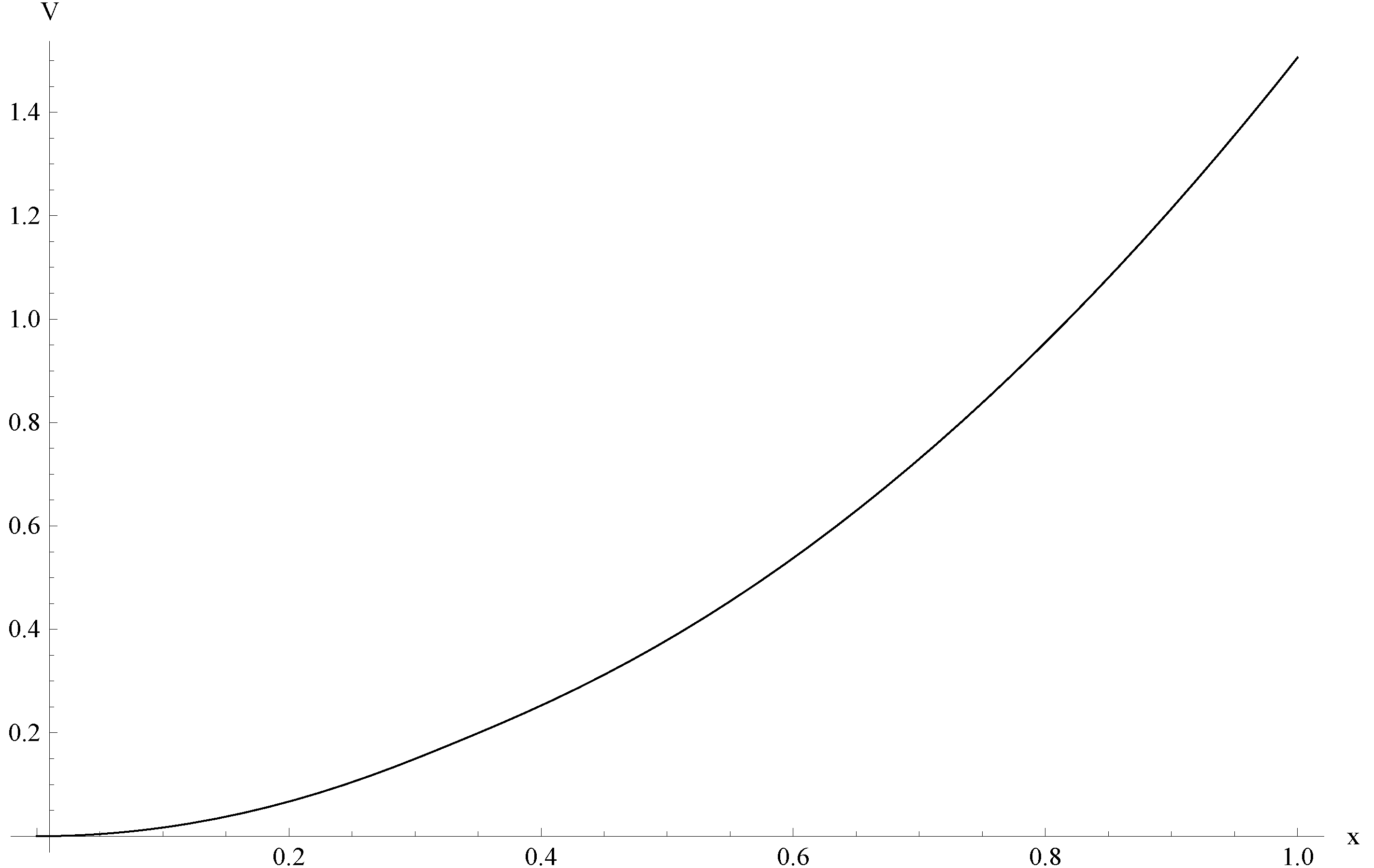
6.1. The Debt Policy Associated with the Optimal Debt Ceiling versus the Non-Intervention Policy

We want to compare the policy obtained in Section 4 with the non-intervention policy. The latter can be modeled as u 0 , that is, u ( t ) = 0 for all t 0 . If the government never intervenes, then
X t = x exp μ 1 2 σ 2 t + σ W t .
The total cost function is
J ( x ; 0 ) = E x 0 e λ t h ( X t ) d t + 0 = E x 0 e λ t α X t m + 1 d t = 0 e λ t α E x X t m + 1 d t = α 0 e λ t x m + 1 exp σ 2 m / 2 + μ t ( m + 1 ) d t = α ξ x m + 1 ,
due to condition (4).
We recall that the value function V represents the minimum expected total discounted cost, and is a function of the initial debt ratio. Thus, the cost J ( x ; 0 ) is greater than or equal to V ( x ) . Indeed, using the parameter values of Example 4 with U ¯ = 0.05 , we plot these functions in Figure 2. We observe that the expected relation is satisfied. Hence, we confirm that it is better to intervene optimally than to not intervene at all. We point out that the larger the initial debt ratio, the greater the benefits of the optimal intervention.

6.2. The Bounded Model versus the Unbounded Model

In this subsection, we compare our results to the ones obtained by Cadenillas and Huamán-Aguilar (2016) for their model with unbounded government intervention. They proved that the optimal debt ceiling b ˜ for the unbounded intervention model is given by
b ˜ = 1 α ξ k ( γ 2 1 ) ( γ 2 m 1 ) ( m + 1 ) 1 m > 0 ,
where
μ ˜ = μ 1 2 σ 2 , γ 2 = μ ˜ + μ ˜ 2 + 2 λ σ 2 σ 2 > 0 , ξ = 1 λ σ 2 m ( m + 1 ) / 2 μ ( m + 1 ) > 0 .
In Table 3, we study the effect of the maximal rate of intervention U ¯ on the optimal debt ceiling. We notice that the optimal debt ceiling b in the bounded model is always smaller than the optimal debt ceiling b ˜ in the unbounded case U ¯ = , given by Equation (59). Moreover, we observe that, as the maximal rate U ¯ increases, the optimal debt ceiling b for the bounded model increases towards the optimal debt ceiling b ˜ for the unbounded model. It is worth remarking that b ˜ is an upper bound for b. Furthermore, we conclude that, other things being equal, countries with severe constraints to control their debt ratios should have low optimal debt ceilings.

6.3. The Effects of α , g, and σ on the Optimal Debt Ceiling

We recall that α represents the importance of government debt. In Table 4 we observe that the more important the government debt, the lower the optimal debt ceiling. In other words, the more concerned the government is about its debt, the more control should be exerted. We note that this result holds for every value of the maximal rate of intervention U ¯ .
We recall the definition μ : = r g in order to analyze the effect of the rate of economic growth. In Table 4, we observe that the larger the rate of economic growth, the larger the optimal debt ceiling. In other words, since the economic growth reduces the debt ratio (see Domar 1944), countries with high economic growth are allowed to have a high debt ceiling. We point out that this behavior holds regardless of the value of the maximal rate of intervention U ¯ .
In Table 4, we also show the effects of volatility. We observe mixed results. If the maximal rate of intervention U ¯ is large, then the higher the debt volatility the larger the optimal debt ceiling. This is consistent with the unbounded model ( U ¯ = ) of Cadenillas and Huamán-Aguilar (2016). However, if the maximal rate of intervention U ¯ is small, then the higher the debt volatility, the lower the optimal debt ceiling. This establishes a dramatic difference with the unbounded model ( U ¯ = ) of Cadenillas and Huamán-Aguilar (2016).
We have also studied the effects of the parameters on the value function. We have found out that an increase in the importance of the debt α for the government, or in the debt volatility σ , implies an increase in the value function, thereby generating a bad result for the government. By contrast, an increase in the rate of economic growth reduces the value function and, hence, improves the government welfare.

7. Summary of Analysis

We have confirmed that the debt policy associated with the optimal debt ceiling is better than the non-intervention policy. Furthermore, as expected, the debt policy associated with the optimal debt ceiling under the bounded intervention model determines a higher cost than the debt policy associated with the optimal debt ceiling for the unbounded intervention model.
In addition, we have studied the time to reach any debt ceiling (including the optimal debt ceiling), when the initial debt ratio is higher than the debt ceiling. We have found out that a country may or may not succeed in reaching its debt ceiling. Indeed, we have found out that countries with strong constraints to generate primary superavits (low maximal rate U ¯ of intervention) may not be able to reduce their debt ratios, and hence may not succeed in reaching their corresponding debt ceilings. On the contrary, for countries with less constraints, we have estimated their finite expected times to reach their debt ceilings. That is, governments that succeed in reducing their debt ratios to their debt ceiling levels do not do so immediately, but over some period of time. These are the main results of this research.
We have observed that our quantitative results are different from those of Cadenillas and Huamán-Aguilar (2016) for the unbounded intervention model ( U ¯ = ). For example, the optimal debt ceiling in our model is smaller than the optimal debt ceiling in the unbounded case. Another important difference is that the optimal debt policies differ and, hence, produce different results. Suppose the initial debt ratio of a country is below the optimal debt ceiling. Then, as pointed out in Section 4.3, sometimes the controlled debt ratio may be above its corresponding optimal debt ceiling, whereas, in the unbounded model, it will always be equal to or less than the optimal debt ceiling.
We have also analyzed the effects of some parameters on the optimal debt ceiling. We have shown that, when the importance of debt for the government increases (large α ), the optimal debt ceiling decreases. An increase in the rate of economic growth (large g) has the same qualitative effect. However, the effect of the volatility ( σ ) on the optimal debt ceiling depends on the maximal rate ( U ¯ ) of intervention. We have shown that, if the maximal rate of intervention U ¯ is large, then the higher the debt volatility, the larger the optimal debt ceiling. Nevertheless, if the maximal rate of intervention U ¯ is small, then the higher the debt volatility, the lower the optimal debt ceiling. This result is different from the one obtained by Cadenillas and Huamán-Aguilar (2016).

8. Conclusions

In this paper, we study the optimal government debt ceiling considering that the generation of primary superavits to reduce the debt ratio is bounded. The goal of the government is to find a debt reduction policy that minimizes the expected total cost, given by the cost of reducing the debt ratio plus the cost (disutility) of having debt. The debt problem is set as a stochastic control problem in continuous time with infinite horizon. We succeed in obtaining the optimal control debt policy. The main contribution of this paper is to present for the first time a model that not only allows us to compute analytically the optimal debt ceiling (as a function of macro-financial variables), but also accounts for the constraints that governments face in reducing their debt ratios. We have shown that this constraint plays a key role in explaining, for instance, why many countries fail to reduce their debt ratios to their debt ceilings.
For future research, it would be interesting to generalize our model to the case in which the interest rate and the GDP growth rate are stochastic processes. This could be complemented by empirical tests.

Author Contributions

A.C. and R.H.-A. have both contributed to this paper.

Funding

The research of Abel Cadenillas was funded by The Social Sciences and Humanities Research Council of Canada, grant number SSHRC IG 435-2017-0511.

Acknowledgments

We dedicate this paper to the memory of Professor Ramón García-Cobián. Preliminary versions of this paper have been presented at ETH (Zurich) Risk Center, Université de Lausanne (Faculté des hautes études commerciales (HEC)), Humboldt Universität zu Berlin, and 2018 INFORMS Informs Annual Meeting. We are grateful to the seminars and conference participants for their comments. We are also grateful for the comments of the associate editor and the five referees.

Conflicts of Interest

The authors declare no conflict of interest. The founding sponsor had no role in the design of the study; in the collection, analyses, or interpretation of data; in the writing of the manuscript, and in the decision to publish the results.

Appendix A. Proof of Proposition 1

Proof. 
Let us consider the controls u 1 and u 2 with u 1 u 2 . Let us denote by X u i the debt ratio controlled by u i , i { 1 , 2 } . Let β ( 0 , 1 ) . From Equation (2), we observe that the debt ratio controlled by β u 1 + ( 1 β ) u 2 is given by
X β u 1 + ( 1 β ) u 2 = β X u 1 + ( 1 β ) X u 2 .
Since h is a strictly convex function,
h ( X t β u 1 + ( 1 β ) u 2 ) = h ( β X t u 1 + ( 1 β ) X t u 2 ) < β h ( X t u 1 ) + ( 1 β ) h ( X t u 2 ) .
Then, for every x ( 0 , ) :
J ( x , β u 1 + ( 1 β ) u 2 ) = E x 0 e λ t h ( X t β u 1 + ( 1 β ) u 2 ) + 0 e λ t k ( β u t 1 + ( 1 β ) u t 2 ) d t < β J ( x ; u 1 ) + ( 1 β ) J ( x ; u 2 ) .
This proves that, if u 1 A ( x ) and u 2 A ( x ) , then β u 1 + ( 1 β ) u 2 A ( x ) . Hence, A ( x ) is a convex set. Furthermore, the function J ( x , · ) is strictly convex.
Suppose that u 1 A ( x ) and u 2 A ( x ) , with u 1 u 2 , are two optimal controls. Then, J ( x ; u 1 ) = J ( x ; u 2 ) ( 0 , ) . Since 1 2 u 1 + 1 2 u 2 A ( x ) and J ( x , · ) is strictly convex,
J x , 1 2 u 1 + 1 2 u 2 < 1 2 J ( x ; u 1 ) + 1 2 J ( x ; u 2 ) = J ( x ; u 1 ) .
This contradicts that u 1 A ( x ) and u 2 A ( x ) are optimal controls. Therefore, Problem 1 has at most one solution. □

Appendix B. Proof of Proposition 2

Proof. 
Since J is nonnegative, the value function V is nonnegative as well.
Consider x 1 < x 2 and u ( 2 ) A ( x 2 ) . Since h is a strictly increasing function, we have
V ( x 1 ) J ( x 1 , u ( 2 ) ) < J ( x 2 , u ( 2 ) ) .
This implies u ( 2 ) A ( x 1 ) and then V ( x 1 ) V ( x 2 ) . Hence, V is increasing.
Consider x 1 x 2 with associated controls u ( 1 ) A ( x 1 ) and u ( 2 ) A ( x 2 ) , and γ [ 0 , 1 ] . We define u ( 3 ) : = γ u ( 1 ) + ( 1 γ ) u ( 2 ) and x 3 : = γ x 1 + ( 1 γ ) x 2 . For every i = 1 , 2 , 3 , we denote by X ( i ) the trajectory that starts at x i and is determined by the control u ( i ) . Thus, for every t 0 :
X t ( 3 ) = γ X t ( 1 ) + ( 1 γ ) X t ( 2 ) .
The convexity of the function h implies
0 e λ t h ( X t ( 3 ) ) d t 0 e λ t γ h ( X t ( 1 ) ) + ( 1 γ ) h ( X t ( 2 ) ) d t = γ 0 e λ t h ( X t ( 1 ) ) d t + ( 1 γ ) 0 e λ t h ( X t ( 2 ) ) d t .
This implies
J ( x 3 ; u ( 3 ) ) γ J ( x 1 ; u ( 1 ) ) + ( 1 γ ) J ( x 2 ; u ( 2 ) ) ,
and hence u ( 3 ) A ( x 3 ) . Thus,
V γ x 1 + ( 1 γ ) x 2 J γ x 1 + ( 1 γ ) x 2 , γ u ( 1 ) + ( 1 γ ) u ( 2 ) = J ( x 3 ; u ( 3 ) ) γ J ( x 1 , u ( 1 ) ) + ( 1 γ ) J ( x 2 , u ( 2 ) ) .
Therefore,
V γ x 1 + ( 1 γ ) x 2 γ V ( x 1 ) + ( 1 γ ) V ( x 2 ) ,
which proves that V is a convex function.
It remains to prove that V ( 0 + ) = 0 . Since V ( x ) is nonnegative, V ( 0 + ) 0 . On the other hand, by the result found in Section 6.1, we have
V ( x ) J ( x ; 0 ) = ξ α x m + 1 ,
which implies V ( 0 + ) 0 . Furthermore, there exists M = ξ α ( 0 , ) such that x ( 0 , ) :
V ( x ) M x m + 1 .
This completes the proof of this proposition. □

Appendix C. Proof of Lemma 2

Proof. 
Let us consider the functions G and H defined by
G ( x ) : = x γ 2 σ 2 2 U ¯ γ 2 K γ 2 , c 2 , x
and
H ( x ) : = 2 U ¯ σ 2 x c 3 K c 3 , 2 c 2 , x .
The function f, defined in (22), can be written as
f ( x ) = j = 0 m + 1 ζ j x j + B 1 G ( x ) + B 2 H ( x ) , x [ b , ) .
By Lemma 1, we note that γ 2 > m + 1 and c 3 > 0 . Then, Remark 2 implies
lim x B 2 H ( x ) = 0 .
Consequently, there exists x ¯ > b , such that for all x > x ¯ , we have 1 < B 2 H ( x ) < 1 . Thus,
f ̲ ( x ) : = j = 0 m + 1 ζ j x j + B 1 G ( x ) 1 < f ( x ) < f ¯ ( x ) : = j = 0 m + 1 ζ j x j + B 1 G ( x ) + 1 .
Since γ 2 > m + 1 , using Remark 2, it follows that G does not satisfy any polynomial growth condition of degree m + 1 . That is, for every M 2 > 0 , there exists x M 2 such that G ( x ) > M 2 ( 1 + x m + 1 ) for every x > x M 2 .
Now, for a contradiction, suppose B 1 > 0 . Then, f ̲ does not satisfy the polynomial growth condition of Lemma 2. However, this, in turn, implies that f does not satisfy that polynomial growth condition either. This contradiction implies that B 1 0 . Next, we show B 1 0 . For a contradiction, suppose B 1 < 0 . Then, there exists x big enough such that f ¯ ( x ) < 0 . However, this contradicts the fact that f is non-negative. Then, there must be the case that B 1 0 . Combining these two results, we conclude that B 1 = 0 . □

Appendix D. Proof of Proposition 3

Proof. 
Proof of Part (i). Since x > c , we can rewrite τ as
τ = inf t > 0 : X t c .
By definition of the debt policy u ( c ) , the debt ratio ceiling follows
X t ( c ) = x + 0 t μ X s ( c ) d s + 0 t σ X s ( c ) d W s U ¯ t .
We define the auxiliary process { Y t } by
Y t = x + 0 t μ Y s d s + 0 t σ Y s d W s ,
and the auxiliary stopping time:
θ : = inf { t > 0 : Y ( t ) c } .
Since U ¯ > 0 , we have X t ( c ) Y t . Then, τ θ . Hence, P x { θ < } P x { τ < } . Thus, it suffices to show that P x { θ < } = 1 .
The stopping time θ can be written as
θ = inf t > 0 : x exp { μ ˜ t + σ W t } c = inf t > 0 : μ ˜ t + σ ( W t ) log x log c .
Since W is also a Brownian motion, the process μ ˜ t + σ ( W t ) is a Brownian motion with drift. We may apply the methods in Section 8.4 of Ross (1996), and Section 7.5 of Karlin and Taylor (1975), to show that if μ ˜ 0 , then P x { θ < } = 1 . This completes the proof of Part (i).
Proof of Part (ii). For < c < x < n < , let us define the auxiliary stopping time
θ ( c , n ) : = inf t > 0 : x + 0 t μ X s ( c ) d s + 0 t σ X s ( c ) d W s U ¯ t ( c , n ) .
We claim that
P x { τ < } = 1 lim n P x { X θ ( c , n ) ( c ) = n } .
Let us prove the claim. We note that, for n N ,
n > c { X θ ( c , n ) ( c ) = c } = { X τ ( c ) = c } = { τ < } .
Since the events in the above union are monotone increasing in n, we have
P x { τ < } = lim n P x { X θ ( c , n ) ( c ) = c } = 1 lim n P x { X θ ( c , n ) ( c ) = n } .
Our goal now is to find an analytic expression for P x { X θ ( c , n ) ( c ) = n } as a function of n, and the other parameters. Let us define the functional f by
f ( x ) : = P x { X θ ( c , n ) ( c ) = n } ,
and the differential operator A by
A ψ ( y ) : = 1 2 σ 2 y 2 d 2 ψ ( y ) d y 2 + μ y U ¯ d ψ ( y ) d y .
According to Section 3, Chapter 15 of Karlin and Taylor (1981), f satisfies the ordinary differential equation,
A f ( y ) = 0 ,
with the boundary conditions f ( c ) = 0 and f ( n ) = 1 . The solution of this differential equation is
f ( x ) = Γ ( α 1 , β / c ) Γ ( α 1 , β / x ) Γ ( α 1 , β / c ) Γ ( α 1 , β / n ) ,
where Γ ( a , z ) is the incomplete Gamma function, defined by
Γ ( a , z ) = z t ( a 1 ) e t d t , z 0 , a > 0 .
Taking the limit, we obtain
lim n f ( x ) = Γ ( α 1 , β / c ) Γ ( α 1 , β / x ) Γ ( α 1 , β / c ) Γ ( α 1 ) .
Here, Γ ( a ) : = Γ ( a , 0 ) , the Gamma function. From Equation (A1), the proof of (53) is complete.
Finally, let us show that
lim U ¯ P x { τ < } = 1 .
By definition of the incomplete Gamma function, we have that Γ ( a , z ) 0 as z . Then, the result follows. □

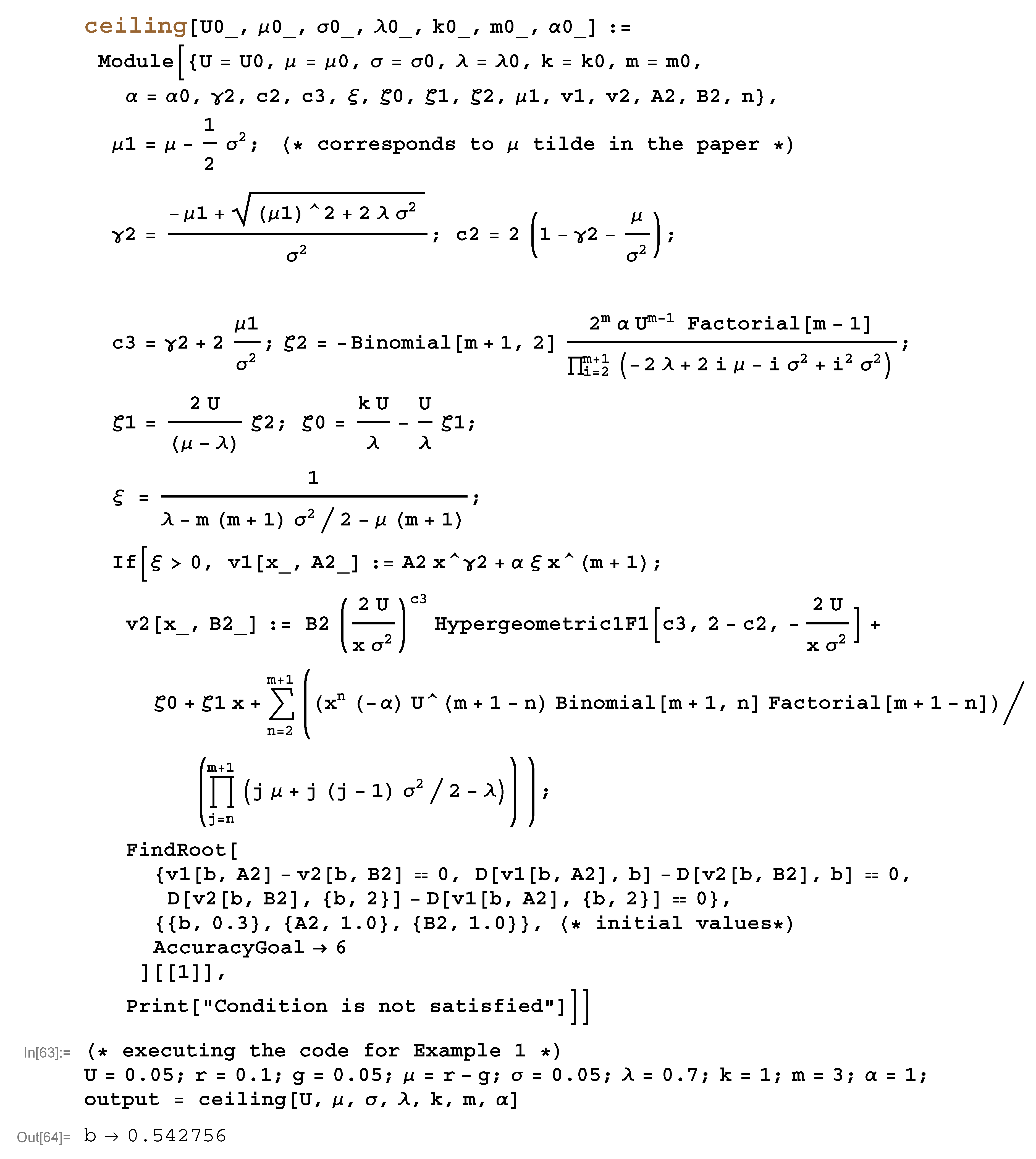
Appendix E. Mathematica Code

Here is the Mathematica 11.0 code for solving numerically Equations (36)–(38). We create the function ceiling whose output is the optimal debt ceiling b. As an illustration, on the bottom part of the code, we apply that function to the parameter values of Example 1.
Risks 06 00138 g0a1

References

  1. Aiyagari, S. Rao, and Ellen R. McGrattan. 1998. The optimum quantity of debt. Journal of Monetary Economics 42: 447–69. [Google Scholar] [CrossRef]
  2. Balassone, Fabrizio, and Daniele Franco. 2000. Assessing fiscal sustainability: A review of methods with a view to EMU. In Fiscal Sustainability. Edited by Banca d’Italia. Rome: Bank of Italy, pp. 21–60. [Google Scholar]
  3. Barro, Robert J. 1989. The Ricardian approach to budget deficits. Journal of Economic Perspectives 3: 37–54. [Google Scholar] [CrossRef]
  4. Barro, Robert J. 1999. Notes on optimal debt management. Journal of Applied Economics 2: 281–89. [Google Scholar]
  5. Bell, William Wallace. 2004. Special Functions for Scientists and Engineers. Mineola: Dover Publications Inc. [Google Scholar]
  6. Blanchard, Olivier J., Jean-Claude Chouraqui, Robert Hagemann, and Nicola Sartor. 1990. The sustainability of fiscal policy: New answers to an old question. OECD Economic Studies 15: 7–36. [Google Scholar]
  7. Blanchard, Olivier. 2017. Macroeconomics, 7th ed. Boston, USA: Pearson Ed. Inc. [Google Scholar]
  8. Bohn, Henning. 1995. The sustainability of budget deficits in a stochastic economy. Journal of Money, Credit, and Banking 27: 257–71. [Google Scholar] [CrossRef]
  9. Brandimarte, Paolo. 2002. Numerical Methods in Finance: A MATLAB-Based Introduction. Hoboken: John Wiley & Sons. [Google Scholar]
  10. Cadenillas, Abel, and Ricardo Huamán-Aguilar. 2016. Explicit formula for the optimal government debt ceiling. Annals of Operations Research 247: 415–49. [Google Scholar] [CrossRef]
  11. Cadenillas, Abel, and Fernando Zapatero. 1999. Optimal Central Bank intervention in the foreign exchange market. Journal of Economic Theory 87: 218–42. [Google Scholar] [CrossRef]
  12. Council of the European Communities. 1992. Treaty on European Union. Brussels and Luxembourg: ECSC-EEC-EAEC. [Google Scholar]
  13. Das, Udaibir S., Michael Papapioannou, Guilherme Pedras, Faisal Ahmed, and Jay Surti. 2010. Managing Public Debt and Its Financial Stability Implications. Working Paper 10/280. Washington, DC, USA: IMF. [Google Scholar]
  14. Domar, Evsey D. 1944. The “Burden of the Debt” and the National Income. The American Economic Review 34: 798–827. [Google Scholar]
  15. Dornbusch, Rudiger, and Mario Draghi, eds. 1990. Public Debt Management: Theory and History. Cambridge: Cambridge University Press. [Google Scholar]
  16. Eaton, Jonathan, and Mark Gersovitz. 1981. Debt with potential repudiation: Theoretical and empirical analysis. Review of Economic Studies 48: 289–309. [Google Scholar] [CrossRef]
  17. Ferrari, Giorgio. 2018. On the Optimal Management of Public Debt: A Singular Stochastic Control Problem. SIAM Journal on Control and Optimization 56: 2036–73. [Google Scholar] [CrossRef]
  18. Fleming, Wendell H., and Halil Mete Soner. 2006. Control Markov Processes and Viscosity Solutions, 2nd ed. New York: Springer. [Google Scholar]
  19. Gersbach, Hans. 2014. Government Debt-Threshold Contracts. Economic Enquiry 52: 444–58. [Google Scholar] [CrossRef]
  20. Ghosh, Atish, Jun I. Kim, Enrique Mendoza, Jonathan Ostry, and Mahvash Qureshi. 2013. Fiscal Fatigue, Fiscal Space and Debt Sustainability in Advanced Economies. The Economic Journal 123: 4–30. [Google Scholar] [CrossRef]
  21. Holmstrong, Bengt, and Jean Tirole. 1998. Private and public supply of liquidity. The Journal of Political Economy 106: 1–40. [Google Scholar] [CrossRef]
  22. Huamán-Aguilar, Ricardo, and Abel Cadenillas. 2015. Government Debt Control: Optimal Currency Portfolio and Payments. Operations Research 63: 1044–57. [Google Scholar] [CrossRef]
  23. IMF and World Bank. 2001. Guidelines for Public Debt Management. Discussion Paper. Washington: IMF and World Bank. [Google Scholar]
  24. IMF and World Bank. 2003. Guidelines for Public Debt Management. Amended Version. Discussion Paper. Washington: IMF and World Bank. [Google Scholar]
  25. IMF. 2002. Assessing Sustainability. Washington: IMF. [Google Scholar]
  26. Karlin, Samuel, and Howard Taylor. 1975. A First Course in Stochastic Processes, 2nd ed. New York: Academic Press. [Google Scholar]
  27. Karlin, Samuel, and Howard Taylor. 1981. A Second Course in Stochastic Processes. New York: Academic Press. [Google Scholar]
  28. Kristensson, Gerhard. 2010. Second Order Differential Equations, Special Functions and Their Classification. New York: Springer. [Google Scholar]
  29. Kydland, Finn E., and Edward C. Prescott. 1977. Rules rather than discretion: The inconsistency of optimal plans. Journal of Political Economy 85: 473–91. [Google Scholar] [CrossRef]
  30. Mas-Colell, Andreu, Michael Dennis Whinston, and Jerry R. Green. 1995. Microeconomic Theory. New York: Oxford University Press. [Google Scholar]
  31. Neck, Reinhard, and Jan-Egbert Sturm, eds. 2008. Sustainability of Public Debt. Cambridge: MIT Press. [Google Scholar]
  32. Ostry, Jonathan David, Atish R. Ghosh, Jun I. Kim, and Mahvash S. Qureshi. 2010. Fiscal Space. Staff Position Paper no SPN/10/11. Washington DC, USA: IMF. [Google Scholar]
  33. Pratt, John W. 1964. Risk aversion in the small and in the large. Econometrica 32: 122–36. [Google Scholar] [CrossRef]
  34. Romer, David. 2002. Advanced Macroeconomics, 2nd ed. New York: McGraw-Hill/Irwin. [Google Scholar]
  35. Ross, Sheldon M. 1996. Stochastic Processes, 2nd ed. New York: John Wiley & Sons, Inc. [Google Scholar]
  36. Shah, Anwar, ed. 2005. Fiscal Management. Washington: The World Bank. [Google Scholar]
  37. Taylor, John B. 1979. Estimation and control of a macroeconomic model with rational expectations. Econometrica 47: 1267–86. [Google Scholar] [CrossRef]
  38. Uctum, Merih, and Michael R. Wickens. 2000. Debt and Deficit Ceilings, and Sustainability of Fiscal Policies: An Intertemporal Analysis. Oxford Bulletin of Economics and Statistics 62: 197–222. [Google Scholar] [CrossRef]
  39. Wheeler, Graeme. 2004. Sound Practice in Government Debt Management. Washington, DC: The World Bank. [Google Scholar]
  40. Woo, Jaejoon, and Manmohan S. Kumar. 2015. Public Debt and Growth. Economica 82: 705–739. [Google Scholar] [CrossRef]
1
That 60 % was simply the median of the debt ratios of those European countries. Although it was not binding, it was considered as a reference value. For more details, please see Footnote 3 of this paper.
2
Optimal debt is the debt ratio that arises as a result of welfare analysis considering that debt, on the one hand, smooths consumption and, on the other hand, has negative effects in wealth distribution; see, for example, Aiyagari and McGrattan (1998) or Barro (1999). Credit ceiling is the level of debt above which the country is not allowed to borrow in the financial markets; see, for example, Eaton and Gersovitz (1981). Debt limit is the debt level at which a debt crises takes place; see, for instance, Ostry et al. (2010).
3
Article 104c of the Maastricht Treaty Council of the European Communities (1992) says the following: “2. The Commission shall monitor the development of the budgetary situation and of the stock of government debt in the Member States with a view to identifying gross errors. In particular, it shall examine compliance with budgetary discipline on the basis of the following two criteria: (a) whether the ratio of the planned or actual government deficit to gross domestic product exceeds a reference value, unless either the ratio has declined substantially and continuously and reached a level that comes close to the reference value;—or, alternatively, the excess over the reference value is only exceptional and temporary and the ratio remains close to the reference value; (b) whether the ratio of government debt to gross domestic product exceeds a reference value, unless the ratio is sufficiently diminishing and approaching the reference value at a satisfactory pace. The reference values are specified in the protocol on the excessive deficit procedure annexed to this Treaty”. In the Maastricht Treaty, the “ratio of the planned or actual government deficit to gross domestic product” is the debt ratio, and the “reference value” is the debt ceiling (which was selected as 60%). Thus, the Maastricht Treaty does not mention explicitly any bound for the government interventions. Similarly, the debate in the USA Senate about the selection of the debt ceiling does not mention any bound for the government interventions.
Figure 1. The value function V.
Risks 06 00138 g001
Figure 2. The value function (for the bounded-intervention model) versus the total cost of the non-intervention policy.
Risks 06 00138 g002
Table 1. Effects of U ¯ on the probability of reaching the debt ceiling c (*).
c Country A Country B
U ¯ = 0.010 0.600.015380.00000
U ¯ = 0.025 0.600.198760.00000
U ¯ = 0.050 0.600.995420.00215
U ¯ = 0.100 0.601.000000.89679
U ¯ = 0.150 0.601.000000.99998
(*) The other parameters used in these computations are those of Example 3.
Table 2. Effects of U ¯ on the probability of reaching the optimal debt ceiling b (*).
b Country A Country B
U ¯ = 0.010 0.609820.023560.00000
U ¯ = 0.025 0.625760.291270.00000
U ¯ = 0.050 0.643240.995980.00215
U ¯ = 0.100 0.654951.000000.89679
U ¯ = 0.150 0.658081.000000.99998
(*) The other parameters used in these computations are those of Example 3, and Equation (57).
Table 3. Effect of U ¯ on the optimal debt ceiling b (*).
U ¯ = 0.001 U ¯ = 0.01 U ¯ = 1 U ¯ = 5 U ¯ =
b0.3000240.3104260.3312130.3313250.331352
(*) The other parameters used in these computations are those of Example 4. The unbounded case U ¯ = is calculated using the explicit Formula (59).
Table 4. Effect of α , μ and σ on the optimal debt ceiling b (*).
α = 0.5 α = 1 α = 1.3
U ¯ = 0.01 0.6098200.3104260.241035
U ¯ = 2.00 0.6624250.3312830.254845
U ¯ = 0.6627040.3313520.254886
μ = 0.05 μ = 0.10 μ = 0.14
U ¯ = 0.01 0.3104260.2639900.253090
U ¯ = 2.00 0.3312830.3034080.282346
U ¯ = 0.3313520.3034660.282397
σ = 0.05 σ = 0.13 σ = 0.17
U ¯ = 0.01 0.3104260.3013630.295110
U ¯ = 2.00 0.3312830.3496970.359007
U ¯ = 0.3313520.3502200.359954
(*) The other parameters used in these computations are those of Example 4. The unbounded case U ¯ = is calculated using the explicit Formula (59).

