A User-Friendly Algorithm for Detecting the Influence of Background Risks on a Model

Abstract

Background, or systematic, risks are integral parts of many systems and models in insurance and finance. These risks can, for example, be economic in nature, or they can carry more technical connotations, such as errors or intrusions, which could be intentional or unintentional. A most natural question arises from the practical point of view: is the given system really affected by these risks? In this paper we offer an algorithm for answering this question, given input-output data and appropriately constructed statistics, which rely on the order statistics of inputs and the concomitants of outputs. Even though the idea is rooted in complex statistical and probabilistic considerations, the algorithm is easy to implement and use in practice, as illustrated using simulated data.

1. Introduction

Actuarial, financial, and economic literature is abundant with models and analyses of background, or systematic, risks that affect decision making (cf., e.g., Finkelshtain et al. 1999; Franke et al. 2006, 2011; Nachman 1982; Pratt 1998; Guo et al. 2018; Furman et al. 2018; and references therein). Various models have been proposed, including additive, multiplicative, and more intricate ones that couple underlying losses (or, generally speaking, inputs) with background risks. For recent far-reaching contributions to this area, we refer to Perote et al. (2015), Su (2016), Su and Furman (2017a, 2017b) Semenikhine et al. (2018), Guo et al. (2018), as well as to the extensive lists of references therein.

Systems and thus their models are prone to a myriad of intentional or unintentional disruptions, which could affect inputs and/or outputs. The literature on the topic is vast, and some of the recent contributions include those tackling deliberate intrusions (e.g., Cárdenas et al. 2011; Premathilaka et al. 2013), and false data injections (e.g., Liang et al. 2017). A number of sophisticated methods have been developed for tackling the problems (e.g., Huang et al. 2016; Onoda 2016; He et al. 2017; Potluri et al. 2017), to name a few.

Whether or not these risks affect the underlying input variables and thus decision making is a problem of immense interest. From the conceptual point of view, broadly speaking, two scenarios arise. First, if it is suspected that the outputs are affected, then testing whether or not this is indeed the case falls, in a sense, within the context of regression analysis, though additional statistical challenges arise (e.g., Perote and Perote-Peña 2004; Perote et al. 2015.; Chen et al. 2018; Gribkova and Zitikis 2018). The second scenario, which is the main topic of the present paper, deals with the case when it is the inputs that are possibly affected by risks.

Statistically speaking, given the input and output random variables X and Y, respectively, which in the risk-free scenario are connected by a “transfer” function h via the equation

$$Y=h(X),$$

(1)

we wish to have an algorithm that would tell us whether risk-free model (1) is true or the risk-contaminated one

$$Y=h(X+\delta ),$$

(2)

where $\delta$ is an exogenous risk, sometimes called input-reading error, that directly affects the input X and thus, indirectly, the output variable as well. We note that Chen et al. (2018) consider model (1) with deterministic inputs, like those to be defined in Equation (3) below. Gribkova and Zitikis (2018) explore risk-free model (1), which can be viewed as the “null hypothesis” in the context of the present paper. Hence, model (2) can be viewed as the “alternative hypothesis,” and the algorithm to be constructed and illustrated in this paper will distinguish between the two hypotheses.

The rest of the paper is organized as follows. In Section 2, we lay out the foundations for assessing the presence, or absence, of input-affecting risks. In Section 3, we describe the algorithm itself. It relies on two statistics whose roles, interrelationship, and asymptotic properties are presented in Section 4 and Section 5. Section 6 concludes the paper with a brief overview of main findings.

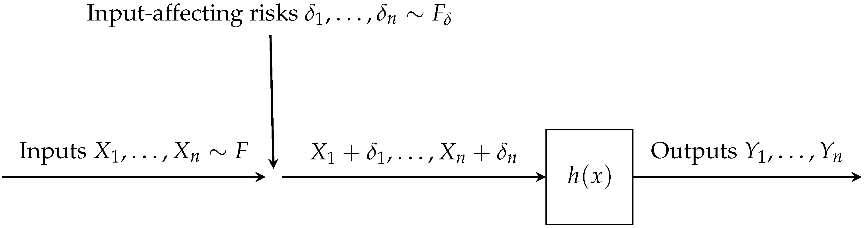
2. The Model

Systems are usually associated with finite-length transfer windows, say $[a,b]\subset \mathbf{R}$, and also with transfer functions $h:[a,b]\to \mathbf{R}$. Let $X_1,\cdots ,X_n$ be input random variables, which we assume to be pre-whitened (e.g., Box et al. 2015), that is, independent and identically distributed (iid). Denote their marginal cumulative distribution functions (cdf) by $F(x)$, whose support is the transfer window $[a,b]$. Hence, the input values are always in $[a,b]$. We assume that the cdf $F(x)$ is strictly increasing on the interval $[a,b]$, with $F(a)=0$ and $F(b)=1$. In fact, to simplify mathematics and still cover a wide variety of applications, we assume that the cdf is continuously differentiable and its probability density function (pdf) is bounded away from 0 on the transfer window $[a,b]$.

Denote the input-affecting risks by ${\delta }_1,\cdots ,{\delta }_n\sim F_{\delta }$, which act upon the inputs $X_1,\cdots ,X_n$ as visualized in Figure 1.

Figure 1. Are the input-affecting risks absent (i.e., degenerate at 0) or not?

We assume that the input-affecting risks are pre-whitened, that is, iid random variables, and we also assume that they are independent of the input variables $X_1,\cdots ,X_n$ and are affecting their values in the additive way. The inputs $X_i$ take values in the interval $[a,b]$, but the risks ${\delta }_i$, being exogenous variables, are not restricted to any domain and can therefore take any real values. Our goal in this paper is to offer a practical way for detecting whether or not the risks are absent, or present. Two following notes relate our research to the topics in statistical literature.

First, the problem that we tackle is different from that dealing with errors-in-variables, where observations already contain errors, whereas in our case, the inputs $X_i$ are uncontaminated but possibly become such while being transferred into the filter, also known as the transmission channel in the engineering literature. That is, in the errors-in-variables scenario, we would observe $X_i+{\delta }_i$, whereas in the present context we observe the original inputs $X_i$ and want to know whether or not they are affected by ${\delta }_i$.

Second, there is a connection between our research and classical regression, and we have already noted contributions by Perote and Perote-Peña (2004), Perote et al. (2015), where we also find extensive lists of related references. Namely, given the outputs $Y_i=h(X_i+{\delta }_i)$ and assuming for the sake of argument that the risks ${\delta }_i$ are small, the Taylor formula gives the approximation $Y_i\approx h(X_i)+h^{\prime }(X_i){\delta }_i$, which places the input-based scenario into the output-based scenario $Y_i=h(X_i)+{\epsilon }_i$, but the risks ${\epsilon }_i\approx h^{\prime }(X_i){\delta }_i$ depend on the inputs $X_i$ via the term $h^{\prime }(X_i)$. This dependence feature presents a major hurdle, which we circumvent in our following considerations and produce a user-friendly algorithm for detecting ${\delta }_i$’s when they are present.

Throughout the paper we assume that the transfer function $h(x)$ has a bounded and continuous first derivative, and we also assume that the derivative is not identically equal to 0, thus ruling out the trivial case of constant transfer functions. Actually, throughout the paper we also exclude the case $h(a)=h(b)$, which causes some technical complications but is hardly of practical relevance, as we shall explain in the next section. If, however, due to some considerations we would need to depart from these conditions, then there is room for relaxing the conditions, though naturally at the expense of more complex considerations.

3. The Algorithm

We first elaborate on the definition of outputs. Indeed, even though $X_i$’s are in the transfer window $[a,b]$, the affected inputs $X_i+{\delta }_i$ may or may not be in $[a,b]$, which is the domain of definition of the transfer function $h(x)$. Hence, the actual outputs are

$$\begin{array}{cc}\hfill Y_i& =h\left(\max \{a,\min \{X_i+{\delta }_i,b\}\}\right)\hfill \\ & =g(X_i+{\delta }_i),i=1,\cdots ,n,\hfill \end{array}$$

where

$$g(x)=h\left(\max \{a,\min \{x,b\}\}\right).$$

Since the cdf of X is continuous, we can uniquely order the random variables $X_1,\cdots ,X_n$. The resulting order statistics $X_{1:n}<\cdots <X_{n:n}$ give rise to the concomitants $Y_{1,n},\cdots ,Y_{n,n}$ (e.g., David and Nagaraja 2003). Based on them and using the notation $x_{+}=\max \{x,0\}$, we define the statistics

$$A_n:=\frac{1}{\sqrt{n}}\sum _{i=2}^n{\left(Y_{i,n}-Y_{i-1,n}\right)}_{+}$$

and

$$B_n:=\frac{1}{\sqrt{n}}\sum _{i=2}^n|Y_{i,n}-Y_{i-1,n}|,$$

and then, in turn, their ratio

$$I_n:=\frac{A_n}{B_n}.$$

The algorithm, to be introduced in a moment, for detecting input-affecting risks is based on asymptotics, when n gets large, of $I_n$ and $B_n$, which we call the pivot and its supporter, thus hinting at their main and supporting roles, respectively. Before formulating the algorithm, we make the natural assumption that the risks, when they exist, should not be so large that the performance of the system would be derailed to such an extent that it becomes unnecessary to run any algorithm. For the purpose of rigour, in the following definition we summarize the circumstances under which there is ambiguity as to the absence, or presence, of input reading risks, and thus employing the algorithm becomes warranted.

Definition 1.

The presence of input-affecting risk is suspected, and thus becomes a subject for testing, when it is believed that there is a set $T\subset [a,b]$ such that the event $X\in T$ has a (strictly) positive probability and, for all $x\in T$, the random variable $g(x+\delta )$ is non-degenerate, due to the random δ.

We note at the outset that Definition 1 is a user-friendly reformulation of technically-looking condition (10) to be presented in Section 5 below, where it plays a pivotal role in setting rigorous mathematical foundations for our algorithm. In this regard, we note that the condition is tightly tied to the indefinite growth of $B_n$ when the sample size n grows, as we shall see in Theorem 3 below. Hence, if the subject-matter knowledge is not sufficiently convincing for the decision maker to see whether or not the circumstances delineated by Definition 1 hold, then data-based checking of the asymptotic behaviour of $B_n$ for large n should clarify the situation.

Definition 1 implies that the system’s output $Y=g(X+\delta )$ varies not just because of X but also because of $\delta$, assuming of course that the latter is present, that is, is not degenerate at 0. This, for example, excludes situations (as unquestionably obvious) when $g(x+\delta )=g(a)$ for every x (i.e., when $-\delta >0$ is very large), or when $g(x+\delta )=g(b)$ for every x (i.e., when $\delta >0$ is very large). In either of these extreme cases, the decision maker would immediately see the system’s malfunction because of the outputs constantly lingering on, or near, the boundaries $g(a)$ and $g(b)$, and thus no special testing would be warranted.

We are now ready to formulate the algorithm for detecting the input-affecting risk when its presence is suspected.

Case 1:

The pivot $I_n$ is not approaching $1/2$.

(i)

If $I_n$ decisively tends to a limit other than $1/2$, then we advise the decision maker about the absence of the risk.

(ii)

If $I_n$ seems to tend to a limit other than $1/2$ but there is some doubt as to whether this is true, then we check if the supporter $B_n$ is asymptotically bounded, and if yes, then we advise the decision maker about the absence of the risk.

Case 2:

The pivot $I_n$ is approaching $1/2$.

(i)

If the supporter $B_n$ tends to infinity, then we advise the decision maker about the presence of the risk.

(ii)

If the supporter $B_n$ is asymptotically bounded, then $h(a)$ and $h(b)$ are likely to be insufficiently different to have already triggered Case 1 above, and we thus advise the decision maker about the absence of the risk.

In the next two sections, we present rigorous results upon which the above algorithm relies. We note in passing that irrespective of whether the algorithm detects risks or not, in either case we can still wish to double-check the findings. It can also be necessary to check the system’s vulnerability (e.g., Hug and Giampapa 2012; and references therein). In such cases, we can use artificially constructed inputs, such as

$$x_{i,n}=a+(b-a)\frac{i-1}{n-1},i=1,\cdots ,n.$$

(3)

We conclude this section with an example that shows how the algorithm works in practice. For this, let the transfer function be $h(x)=1-{(x-0.25)}^2$ for $x\in [0,1]$. Furthermore, upon recalling that the (unconditional) Lomax cdf is ${1-(1+x/\beta ))}^{-\alpha }$ for $x\ge 0$, with shape and scale parameters $\alpha >0$ and $\beta >0$, we assume that the input X follows the $\mathrm{Lomax}(\alpha ,\beta )$ distribution conditioned on the transfer interval $[0,1]$. Throughout the illustration, we set $\alpha =1.5$ and $\beta =1$.

Let $\delta$ follow the normal distributions with the mean 0 and standard deviation $\sigma$. In the risk-free case (i.e., $\sigma =0$), the asymptotics of $I_n$ and $B_n$ is depicted in panels (a) and (b) of Figure 2, and when $\sigma =0.1$, their asymptotics is depicted in panels (c) and (d). We also check the performance of the algorithm when the risk $\delta$ is discrete, specifically, when it is equal to $-2$ with probability $0.7$ and to 2 with probability $0.3$. The asymptotics of $I_n$ and $B_n$ is depicted in panels (e) and (f) of Figure 2.

Figure 2. $B_n$ for discrete $\pm 2$ risk.

We see from the left-hand panels that the pivot $I_n$ converges to the limit other than $1/2$ (i.e., to the value of $I_h$ to be defined by Equation (4) in the next section) only in the risk-free case. The increasing pattern of $B_n$ in panels (d) and (f) confirms the presence of input risk in both scenarios, which have initially been detected by the pivot $I_n$ (due to its convergence to $1/2$) in panels (c) and (e). Note that the convergence to $1/2$ in panel (e) is decisive, whereas the convergence in panel (c) may not be so well pronounced, and thus the increasing pattern of $B_n$ in panel (d) provides reassurance.

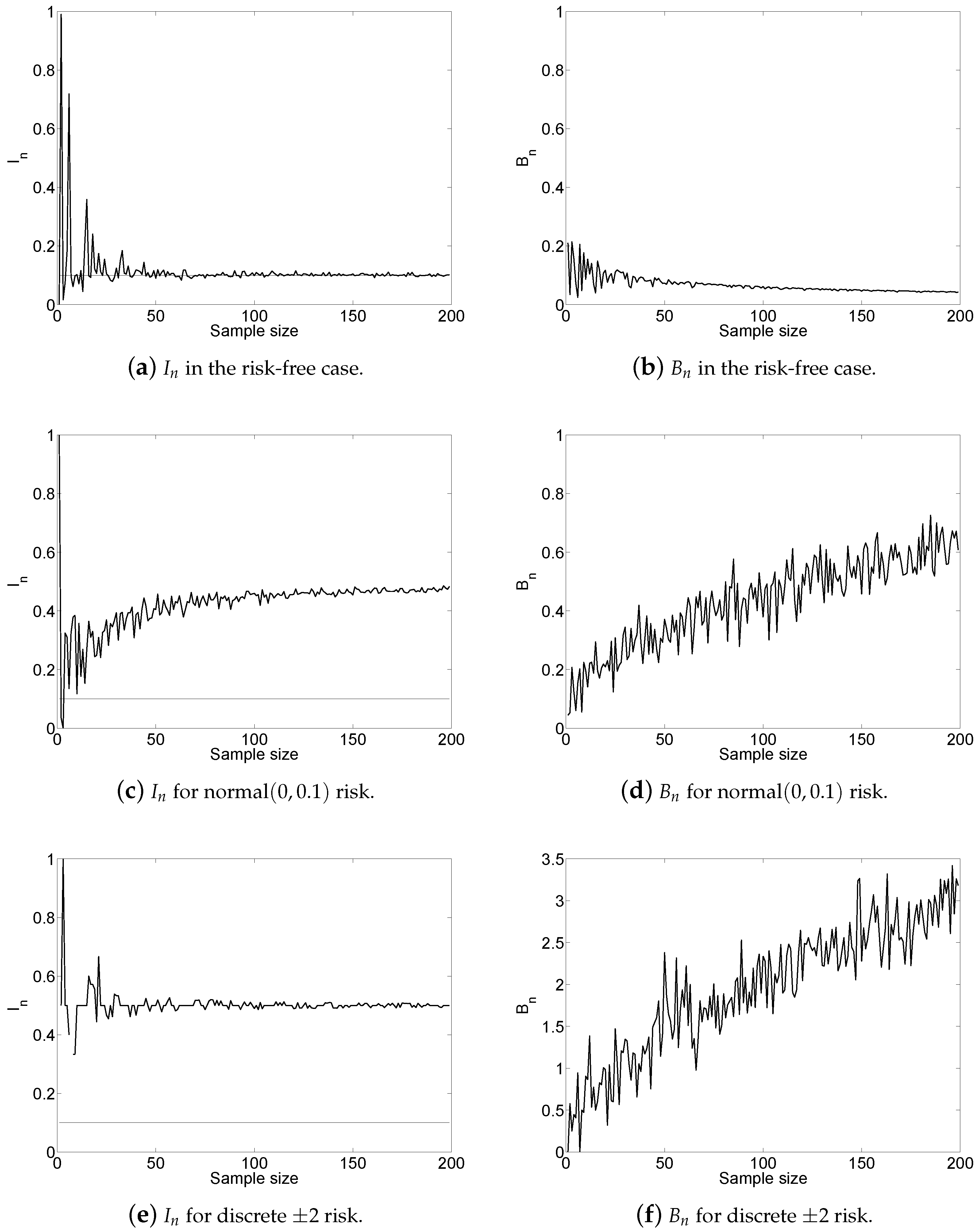
4. Asymptotics of the Pivot ${\mathit{I}}_{\mathit{n}}$

We begin with the case when the input-affecting risk is absent, and thus the system is functioning properly. This is the starting point of many works (e.g., Cárdenas et al. 2011, p. 360) dealing with intrusion detection (e.g., Debar et al. 1999; Premathilaka et al. 2013), false data injections (e.g., Liang et al. 2017), and other disruptions. Recall the notation $x_{+}=\max \{x,0\}$ for any $x\in \mathbf{R}$.

Theorem 1

(Gribkova and Zitikis, 2018). If δ is absent, then, when $n\to \infty$, the pivot $I_n$ converges to

$$I_h:=\frac{{\int }_a^b{(h^{\prime }(u))}_{+}\mathrm{d}u}{{\int }_a^b\left|h^{\prime }(u)\right|\mathrm{d}u}.$$

(4)

For another perspective on the meaning of $I_h$, we refer to Davydov and Zitikis (2017) where $I_h$ arises as the solution to an optimization problem. The importance of Theorem 1 in the present paper follows from the fact that when the cdf $F_{\delta }$ is non-degenerate, then (details in Section 5 below) the pivot $I_n$ converges to $1/2$ when $n\to \infty$. Of course, the limit $1/2$ can also manifest when $\delta$ is absent, that is, in the context of Theorem 1, but this can happen only when $h(a)=h(b)$. Indeed, as it is easy to check using the equations $|x|=x_{+}+x_{-}$ and $x=x_{+}-x_{-}$ with $x_{-}=\max \{-x,0\}$, we have $I_h=1/2$ if and only if $h(a)=h(b)$. The latter property is, however, an exception rather than the rule: it manifests in such cases when, for example, the system is down and thus $h(x)$ takes the same value irrespective of $x\in [a,b]$. Hence, unless explicitly noted otherwise, throughout the paper we assume

$$h(a)\ne h(b),$$

(5)

as we have already mentioned earlier.

We next discuss how to check whether or not the risk $\delta$ is degenerate. Naturally, in order to detect anomalies, the original state of the system has to be in reasonable working order (cf., e.g., Cárdenas et al. 2011, p. 360). Gribkova and Zitikis (2018) have put forward an argument in favour of the following definition.

Definition 2.

A system is in reasonable working order whenever in the absence of input-affecting risk (i.e., when $\delta =0$ almost surely), the sequence $B_n$ is asymptotically bounded in probability. In mathematical terms, we write this as $B_n=O_{\mathbf{P}}(1)$ when $n\to \infty$.

Given that in the absence of input-affecting risk we are exploring the asymptotic behaviour of the pivot $I_n$, which is the ratio of $A_n$ and $B_n$, both of which are asymptotically bounded in probability, the requirement $B_n=O_{\mathbf{P}}(1)$ is natural. This can be seen from the following argument involving the mean-value theorem:

$$\begin{array}{cc}\hfill \frac{1}{\sqrt{n}}\sum _{i=2}^n|h(X_{i:n})-h(X_{i-1:n})|& =\frac{1}{\sqrt{n}}\sum _{i=2}^n\left|h^{\prime }({\xi }_i)\left(X_{i:n}-X_{i-1:n}\right)\right|\hfill \\ & \le \frac{\parallel h^{\prime }\parallel (b-a)}{\sqrt{n}}\hfill \end{array}$$

(6)

for some ${\xi }_i$ between $X_{i-1:n}$ and $X_{i:n}$, where

$$\parallel h^{\prime }\parallel :=\underset{a\le x\le b}{\sup }\left|h^{\prime }(x)\right|<\infty .$$

As a side-note, the right-hand side of bound (6) implies that, if needed, the boundedness of the first derivative of the transfer function can be relaxed and the system can still remain in reasonable working order, as per Definition 2.

We next present an example that shows what happens with the system when the input-affecting risk is present, that is, when the cdf $F_{\delta }$ is non-degenerate. Before starting the example, we recall (David and Nagaraja 2003) that the concomitants $Y_{1,n},\cdots ,Y_{n,n}$ can be written as follows

$$Y_{i,n}=g\left(X_{i:n}+{\delta }_{[i]}\right),$$

where ${\delta }_{[i]}$ is the random variable among ${\delta }_1,\cdots ,{\delta }_n$ that corresponds to $X_{i:n}$. As noted by David and Nagaraja (2003, p. 145), the random variables ${\delta }_{[1]},\cdots ,{\delta }_{[n]}$ are iid and follow the cdf $F_{\delta }$ of the original risk $\delta$.

Example 1.

Let δ take value $c>0$ with probability $p\in (0,1)$ and $-c$ with probability $1-p$, and let $c\ge b-a$. The latter assumption implies that irrespective of the value of $X_{i:n}$, the value of $X_{i:n}+{\delta }_{[i]}$ is above b with probability p and below a with probability $1-p$. Hence, the concomitant $Y_{i,n}$ is equal to $h(b)$ with probability p and to $h(a)$ with probability $1-p$. Since each concomitant can take only two values, $|Y_{i,n}-Y_{i-1,n}|$ is equal to $|h(b)-h(a)|$ when ${\delta }_{[i]}\ne {\delta }_{[i-1]}$ and 0 otherwise. Consequently,

$$|Y_{i,n}-Y_{i-1,n}|=\frac{|h(b)-h(a)|}{2c}|{\delta }_{[i]}-{\delta }_{[i-1]}|,$$

which implies

$$\begin{array}{cc}\hfill B_n& =\frac{|h(b)-h(a)|}{2c}\left\{\frac{1}{\sqrt{n}}\sum _{i=2}^n\left(|{\delta }_{[i]}-{\delta }_{[i-1]}|-\mathbf{E}\left[|{\delta }_{[i]}-{\delta }_{[i-1]}|\right]\right)+\frac{n-1}{\sqrt{n}}\mathbf{E}\left[|{\delta }_{[i]}-{\delta }_{[i-1]}|\right]\right\}\hfill \\ & =\frac{|h(b)-h(a)|}{2c}\sqrt{n}\mathbf{E}\left[|{\delta }_{[i]}-{\delta }_{[i-1]}|\right]+O_{\mathbf{P}}(1).\hfill \end{array}$$

(7)

Since the variables ${\delta }_{[1]},\cdots ,{\delta }_{[n]}$ are iid and follow the same cdf $F_{\delta }$ as the original δ, the mean $\mathbf{E}[|{\delta }_{[i]}-{\delta }_{[i-1]}|]$ is equal to $4cp(1-p)$ and thus Equation (7) implies

$$B_n=2\sqrt{n}p(1-p)|h(b)-h(a)|+O_{\mathbf{P}}(1).$$

(8)

From this we conclude that if p is neither 0 nor 1, which we assume, and if $h(b)\ne h(a)$, which we also assume, then $B_n\stackrel{\mathbf{P}}{\to }\infty$ when $n\to \infty$. Analogous arguments lead to

$$A_n=\sqrt{n}p(1-p)|h(b)-h(a)|+O_{\mathbf{P}}(1).$$

(9)

Combining statements (8) and (9), we have $I_n=A_n/B_n\stackrel{\mathbf{P}}{\to }1/2$ when $n\to \infty$, which in turn implies that the system is affected by the risk. This concludes Example 1.

The above example has been constructed to show—in a somewhat dramatic way—what happens when the input-affecting risk pushes the input outside the transfer window, but the same conclusion can be reached under much weaker assumptions on $\delta$, as we shall show in the next section.

5. Growth of the Supporter ${\mathit{B}}_{\mathit{n}}$

The following general result plays a major role in the justification of the earlier presented algorithm.

Theorem 2.

Gribkova and Zitikis (2018) Let $(X_1,Y_1),\cdots ,(X_n,Y_n)$ be independent copies of a generic random pair $(X,Y)$, with X having continuous cdf and Y having finite second moment. If $B_n\stackrel{\mathbf{P}}{\to }\infty$, then $I_n\stackrel{\mathbf{P}}{\to }1/2$ when $n\to \infty$.

We know from statement (6) and the arguments around it that if $\delta$ is degenerate, then $B_n\stackrel{\mathbf{P}}{\to }\infty$ cannot be true. In the next theorem, we give a necessary and sufficient condition for $B_n\stackrel{\mathbf{P}}{\to }\infty$ to hold, which, according to Theorem 2, implies $I_n\stackrel{\mathbf{P}}{\to }1/2$.

Theorem 3.

The statement $B_n\stackrel{\mathbf{P}}{\to }\infty$ holds if and only if

$${\int }_0^1(2t-1)\left({\int }_0^1{F}_{g(x_s+\delta )}^{-1}(t)\mathrm{d}s\right)\mathrm{d}t>0,$$

(10)

where $x_s=F^{-1}(s)$ is the $sth$ percentile of X, and $F_{g(x_s+\delta )}^{-1}(t)$ denotes the quantile function of the random variable $g(x_s+\delta )$.

Condition (10) arises naturally, but its formulation is not user friendly. Remarkably, its meaning is very simple and has already been conveyed in Definition 1. Before proving Theorem 3, we next illuminate the meaning of condition (10) by revisiting Example 1 through the lens of the condition.

Example 2.

Let δ take value $c>0$ with probability $p\in (0,1)$ and $-c$ with probability $1-p$, and let $c\ge b-a$. Since for every $s\in (0,1)$ we have $x_s=F^{-1}(s)\in [a,b]$, the random variable $g(x_s+\delta )$ has the probability distribution

$$g(x_s+\delta )=\left\{\begin{array}{cc}h(a)\hfill & withprobability1-p,\hfill \\ h(b)\hfill & withprobabilityp.\hfill \end{array}\right.$$

To obtain its quantile function, we start with the case $h(a)\le h(b)$ and have the formula

$$F_{g(x_s+\delta )}^{-1}(t)=\left\{\begin{array}{cc}h(a)\hfill & when0<t\le 1-p,\hfill \\ h(b)\hfill & when1-p<t\le 1.\hfill \end{array}\right.$$

Consequently,

$$\begin{array}{cc}\hfill {\int }_0^1(2t-1)\left({\int }_0^1{F}_{g(x_s+\delta )}^{-1}(t)\mathrm{d}s\right)\mathrm{d}t& =h(a){\int }_0^{1-p}(2t-1)\mathrm{d}t+h(b){\int }_{1-p}^1(2t-1)\mathrm{d}t\hfill \\ & =p(1-p)\left(h(b)-h(a)\right).\hfill \end{array}$$

Analogous calculations when $h(a)\ge h(b)$ give the answer $p(1-p)(h(a)-h(b))$, thus establishing the equation

$${\int }_0^1(2t-1)\left({\int }_0^1{F}_{g(x_s+\delta )}^{-1}(t)\mathrm{d}s\right)\mathrm{d}t=p(1-p)|h(b)-h(a)|$$

irrespective of the values of $h(a)$ and $h(b)$. We can therefore conclude that as long as $h(b)\ne h(a)$ and p is neither 0 nor 1, condition (10) is satisfied. Thus, we have $B_n\stackrel{\mathbf{P}}{\to }\infty$ according to Theorem 3.

Proof of Theorem 3.

We first show that if condition (10) is satisfied, then $B_n\stackrel{\mathbf{P}}{\to }\infty$. We start with the bound

$$\begin{array}{cc}\hfill B_n& =\frac{1}{\sqrt{n}}\sum _{i=2}^n|g(X_{i:n}+{\delta }_{[i]})-g(X_{i-1:n}+{\delta }_{[i-1]})|\hfill \\ & \ge \frac{1}{\sqrt{n}}\sum _{i=2}^n|g(X_{i-1:n}+{\delta }_{[i]})-g(X_{i-1:n}+{\delta }_{[i-1]})|-\frac{1}{\sqrt{n}}\sum _{i=2}^n|g(X_{i:n}+{\delta }_{[i]})-g(X_{i-1:n}+{\delta }_{[i]})|.\hfill \end{array}$$

(11)

Since the transfer function $h(x)$ has a bounded derivative on the interval $[a,b]$, the function $g(x)$ is Lipschitz continuous on the entire real line, that is, $|g(x)-g(y)|\le \parallel h^{\prime }\parallel |x-y|$ for all $x,y\in \mathbf{R}$. Continuing with bound (11), we have

$$\begin{array}{cc}\hfill B_n& \ge \frac{1}{\sqrt{n}}\sum _{i=2}^n|g(X_{i-1:n}+{\delta }_{[i]})-g(X_{i-1:n}+{\delta }_{[i-1]})|-\frac{\parallel h^{\prime }\parallel (b-a)}{\sqrt{n}}\hfill \\ & =\frac{1}{\sqrt{n}}\sum _{i=2}^n|g(X_{i-1}+{\delta }_i)-g(X_{i-1}+{\delta }_{i-1})|-\frac{\parallel h^{\prime }\parallel (b-a)}{\sqrt{n}}\hfill \\ & =\frac{n-1}{\sqrt{n}}\mathbf{E}\left[|g(X+{\delta }_2)-g(X+{\delta }_1)|\right]-\frac{\parallel h^{\prime }\parallel (b-a)}{\sqrt{n}}+O_{\mathbf{P}}(1),\hfill \end{array}$$

(12)

because (i) the inputs $X_i$ and the risks ${\delta }_i$ are independent, (ii) the inputs $X_i$ have the same cdf F, and (iii) the risks ${\delta }_i$ have the same cdf $F_{\delta }$. Hence, if the expectation on the right-hand side of bound (12) does not vanish, then we must have $B_n\stackrel{\mathbf{P}}{\to }\infty$ when $n\to \infty$. The proof of the converse (i.e., if $B_n\stackrel{\mathbf{P}}{\to }\infty$, then condition (13) is satisfied) follows from the same arguments but now with “+” instead of “−” and the reversed inequalities in bounds (11) and (12).

We are left to show that the statement

$$\mathbf{E}\left[|g(X+{\delta }_2)-g(X+{\delta }_1)|\right]>0$$

(13)

holds if and only if condition (10) is satisfied. We do so with the help of the equation

$$\mathbf{E}\left[|g(X+{\delta }_2)-g(X+{\delta }_1)|\right]=2{\int }_0^1(2t-1)\left({\int }_{\mathbf{R}}{F}_{g(x+\delta )}^{-1}(t)\mathrm{d}F(x)\right)\mathrm{d}t,$$

(14)

which trivially follows from

$$\begin{array}{c}\hfill \mathbf{E}\left[|g(X+{\delta }_2)-g(X+{\delta }_1)|\right]=\mathbf{E}\left[\mathrm{GMD}(X)\right]\\ \hfill ={\int }_0^1\mathrm{GMD}(x_s)\mathrm{d}s,\end{array}$$

where $\mathrm{GMD}(x)$ is the Gini mean difference of the variable $g(x+\delta )$, defined by

$$\begin{array}{cc}\hfill \mathrm{GMD}(x)& :=\mathbf{E}\left[|g(x+{\delta }_2)-g(x+{\delta }_1)|\right]\hfill \\ & =2{\int }_0^1(2t-1)F_{g(x+\delta )}^{-1}(t)\mathrm{d}t.\hfill \end{array}$$

The right-most equation holds due to the well-known representation of the Gini mean difference as a Choquet integral (e.g., Giorgi 1993; Yitzhaki and Schechtman 2013; Furman et al. 2017; and references therein). We conclude with the note that the Gini mean difference is known to be (strictly) positive whenever the underlying random variable is non-degenerate, which in our case is $g(x+\delta )$. Hence, by assuming non-degeneracy of $g(x+\delta )$ for every $x\in T\subseteq [a,b]$ such that $\mathbf{P}[X\in T]>0$, we arrive at condition (13) and thus, in turn, at (10). The proof of Theorem 3 is finished. ☐

6. Concluding Notes

The need for an algorithm that distinguishes between the “null hypothesis” $Y=g(X)$ and the “alternative” $Y=g(X+\delta )$ for exogenous background risk $\delta$ arises in many problems of economics, insurance, and finance. In the present paper, we have developed a user-friendly algorithm for distinguishing between the aforementioned two hypotheses. The algorithm is based on the asymptotic behaviour of two statistics: the pivot $I_n$ and its supporter $B_n$, which are constructed using the order statistics of inputs and the corresponding concomitants of outputs. We have supplemented our theoretical considerations with illustrative examples, graphs, and discussions, thus facilitating the use of the algorithm in practice.

As we have noted in the Introduction, practical considerations give rise to alternatives which couple X and $\delta$ not just in the additive way but possibly in a more intricate way, which we generally formulate as $Y=g(X,\delta )$. In this regard we also note that X and $\delta$ might be dependent random variables, and even multivariate ones, thus giving rise to a highly non-trivial follow-up problem.

References

- Box, George Edward Pelham, Gwilym Meirion Jenkins, Gregory C. Reinsel, and Greta M. Ljung. 2015. Time Series Analysis: Forecasting and Control, 5th ed. New York: Wiley. [Google Scholar]
- Cárdenas, Alvaro A., Saurabh Amin, Zong-Syun Lin, Yu-Lun Huang, Chi-Yen Huang, and Shankar Sastry. 2011. Attacks against process control systems: Risk assessment, detection, and response. Paper presented at the 6th ACM Symposium on Information, Computer and Communications Security, Hong Kong, March 22–24; pp. 355–66. [Google Scholar]
- Chen, Lingzhi, Youri Davydov, Nadezhda Gribkova, and Ričardas Zitikis. 2018. Estimating the index of increase via balancing deterministic and random data. Mathematical Methods of Statistics 27: 83–102. [Google Scholar] [CrossRef]
- David, Herbert A., and Haikady N. Nagaraja. 2003. Order Statistics, 3rd ed. New York: Wiley. [Google Scholar]
- Davydov, Youri, and Ričardas Zitikis. 2017. Quantifying non-monotonicity of functions and the lack of positivity in signed measures. Modern Stochastics: Theory and Applications 4: 219–31. [Google Scholar] [CrossRef]
- Debar, Hervé, Marc Dacier, and Andreas Wespi. 1999. Towards a taxonomy of intrusion-detection systems. Computer Networks 31: 805–22. [Google Scholar] [CrossRef]
- Finkelshtain, Israel, Offer Kella, and Marco Scarsini. 1999. On risk aversion with two risks. Journal of Mathematical Economics 31: 239–50. [Google Scholar] [CrossRef]
- Franke, Günter, Harris Schlesinger, and Richard C. Stapleton. 2006. Multiplicative background risk. Management Science 52: 146–53. [Google Scholar] [CrossRef]
- Franke, Günter, Harris Schlesinger, and Richard C. Stapleton. 2011. Risk taking with additive and multiplicative background risks. Journal of Economic Theory 146: 1547–68. [Google Scholar] [CrossRef]
- Furman, Edward, Ruodu Wang, and Zitikis ardas. 2017. Gini-type measures of risk and variability: Gini shortfall, capital allocations, and heavy-tailed risks. Journal of Banking and Finance 83: 70–84. [Google Scholar] [CrossRef]
- Furman, Edward, Alexey Kuznetsov, and Ričardas Zitikis. 2018. Weighted risk capital allocations in the presence of systematic risk. Insurance: Mathematics and Economics 79: 75–81. [Google Scholar]
- Giorgi, Giovanni. 1993. A fresh look at the topical interest of the Gini concentration ratio. Metron 51: 83–98. [Google Scholar]
- Gribkova, Nadezhda, and Ričardas Zitikis. 2018. Assessing transfer functions in control systems. arXiv, arXiv:1805.10633. [Google Scholar]
- Guo, Xu, Andreas Wagener, Wing-Keung Wong, and Lixing Zhu. 2018. The two-moment decision model with additive risks. Risk Management 20: 77–94. [Google Scholar] [CrossRef]
- Guo, Xu, Raymond Honfu Chan, Wing-Keung Wong, and Lixing Zhu. 2018. Mean-variance, mean-VaR, and mean-CVaR models for portfolio selection with background risk. Risk Management. [Google Scholar] [CrossRef]
- He, Youbiao, Gihan J. Mendis, and Jin Wei. 2017. Real-rime detection of false data injection attacks in smart grid: A deep learning-based intelligent mechanism. IEEE Transactions on Smart Grid 8: 2505–16. [Google Scholar] [CrossRef]
- Huang, Yi, Jin Tang, Yu Cheng, Husheng Li, Kristy A. Campbell, and Zhu Han. 2016. Real-time detection of false data injection in smart grid networks: An adaptive CUSUM method and analysis. IEEE Systems Journal 10: 532–43. [Google Scholar] [CrossRef]
- Hug, Gabriela, and Joseph Andrew Giampapa. 2012. Vulnerability assessment of AC state estimation with respect to false data injection cyber-attacks. IEEE Transactions on Smart Grid 3: 1362–70. [Google Scholar] [CrossRef]
- Liang, Gaoqi, Junhua Zhao, Fengji Luo, Steven R. Weller, and Zhao Yang Dong. 2017. A review of false data injection attacks against modern power systems. IEEE Transactions on Smart Grid 8: 1630–38. [Google Scholar] [CrossRef]
- Nachman, David. 1982. Preservation of “more risk averse” under expectations. Journal of Economic Theory 28: 361–68. [Google Scholar] [CrossRef]
- Onoda, Takashi. 2016. Probabilistic models-based intrusion detection using sequence characteristics in control system communication. Neural Computing and Applications 27: 1119–27. [Google Scholar] [CrossRef]
- Perote, Javier, and Juan Perote-Peña. 2004. Strategy-proof estimators for simple regression. Mathematical Social Sciences 47: 153–76. [Google Scholar] [CrossRef]
- Perote, Javier, Juan Perote-Peña, and Marc Vorsatz. 2015. Strategic behavior in regressions: An experimental study. Theory and Decision 79: 517–46. [Google Scholar] [CrossRef]
- Potluri, Sasanka, Christian Diedrich, and Girish Kumar Reddy Sangala. 2017. Identifying false data injection attacks in industrial control systems using artificial neural networks. Paper presented at the 22nd IEEE International Conference on Emerging Technologies and Factory Automation, Limassol, Cyprus, December 21; pp. 1–8. [Google Scholar]
- Pratt, John W. 1998. Aversion to one risk in the presence of others. Journal of Risk and Uncertainty 1: 395–413. [Google Scholar] [CrossRef]
- Premathilaka, Nalaka Arjuna, Achala Chathuranga Aponso, and Naomi Krishnarajah. 2013. Review on state of art intrusion detection systems designed for the cloud computing paradigm. Paper presented at 47th International Carnahan Conference on Security Technology, Medellin, Colombia, October 8–11; pp. 1–6. [Google Scholar]
- Semenikhine, Vadim, Edward Furman, and Jianxi Su. 2018. On a multiplicative multivariate gamma distribution with applications in insurance. Risks 6: 79. [Google Scholar] [CrossRef]
- Su, Jianxi. 2016. Multiple Risk Factors Dependence Structures with Applications to Actuarial Risk Management. Ph.D. Dissertation, York University, Toronto, ON, Canada. [Google Scholar]
- Su, Jianxi, and Edward Furman. 2017a. A form of multivariate Pareto distribution with applications to financial risk measurement. ASTIN Bulletin 47: 331–57. [Google Scholar] [CrossRef]
- Su, Jianxi, and Edward Furman. 2017b. Multiple risk factor dependence structures: Distributional properties. Insurance: Mathematics and Economics 76: 56–68. [Google Scholar] [CrossRef]
- Yitzhaki, Shlomo, and Edna Schechtman. 2013. The Gini Methodology: A Primer on a Statistical Methodology. New York: Springer. [Google Scholar]
© 2018 by the authors. Licensee MDPI, Basel, Switzerland. This article is an open access article distributed under the terms and conditions of the Creative Commons Attribution (CC BY) license (http://creativecommons.org/licenses/by/4.0/).
Share and Cite
Gribkova, N.; Zitikis, R. A User-Friendly Algorithm for Detecting the Influence of Background Risks on a Model. Risks 2018, 6, 100. https://doi.org/10.3390/risks6030100
Gribkova N, Zitikis R. A User-Friendly Algorithm for Detecting the Influence of Background Risks on a Model. Risks. 2018; 6(3):100. https://doi.org/10.3390/risks6030100
Chicago/Turabian StyleGribkova, Nadezhda, and Ričardas Zitikis. 2018. "A User-Friendly Algorithm for Detecting the Influence of Background Risks on a Model" Risks 6, no. 3: 100. https://doi.org/10.3390/risks6030100
APA StyleGribkova, N., & Zitikis, R. (2018). A User-Friendly Algorithm for Detecting the Influence of Background Risks on a Model. Risks, 6(3), 100. https://doi.org/10.3390/risks6030100