The Cascade Bayesian Approach: Prior Transformation for a Controlled Integration of Internal Data, External Data and Scenarios

Abstract

According to the last proposals of the Basel Committee on Banking Supervision, banks or insurance companies under the advanced measurement approach (AMA) must use four different sources of information to assess their operational risk capital requirement. The fourth includes ’business environment and internal control factors’, i.e., qualitative criteria, whereas the three main quantitative sources available to banks for building the loss distribution are internal loss data, external loss data and scenario analysis. This paper proposes an innovative methodology to bring together these three different sources in the loss distribution approach (LDA) framework through a Bayesian strategy. The integration of the different elements is performed in two different steps to ensure an internal data-driven model is obtained. In the first step, scenarios are used to inform the prior distributions and external data inform the likelihood component of the posterior function. In the second step, the initial posterior function is used as the prior distribution and the internal loss data inform the likelihood component of the second posterior function. This latter posterior function enables the estimation of the parameters of the severity distribution that are selected to represent the operational risk event types.

1. Introduction

Basel II capital accord defines the capital charge as a risk measure obtained on an annual basis at a given confidence level on a loss distribution that integrates the following four sources of information: internal data, external data, scenario analysis, business environment and internal control factors (see Box 1).

Box 1. Mixing of outcomes from AMA sub-models. 

‘258. The Range of Practice Paper recognises that “there are numerous ways that the four data elements have been combined in AMA capital models and a bank should have a clear understanding of the influence of each of these elements in their capital model”. In some cases, it may not be possible to:

(a) Perform separate calculations for each data element; or

(b) Precisely evaluate the effect of gradually introducing the different elements.

259. While, in principle, this may be a useful mathematical approach, certain approaches to modelling may not be amenable to this style of decomposition. However, regardless of the modelling approach, a bank should have a clear understanding of how each of the four data elements influences the capital charge.

260. A bank should avoid arbitrary decisions if they combine the results from different sub-models within an AMA model. For example, in a model where internal and external loss data are modelled separately and then combined, the blending of the output of the two models should be based on a logical and sound statistical methodology. There is no reason to expect that arbitrarily weighted partial capital requirement estimates would represent a bank’s requisite capital requirements commensurate with its operational risk profile. Any approach using weighted capital charge estimates needs to be defensible and supported, for example by thorough sensitivity analysis that considers the impact of different weighting schemes.’ BCBS (2010)

Basel II and Solvency II require financial institutions to access the capital charge associated with operational risks BCBS (2001, 2010). There are three different approaches to measure operational risks, namely the basic, the standard and the advanced measurement approach (AMA), representing increasing levels of control and the difficulty of implementation. The AMA requires a better understanding of the exposure for implementing an internal model.

Basel II capital accord defines the capital charge as a risk measure obtained on an annual basis at a given confidence level on a loss distribution that integrates the following four sources of information: internal data, external data, scenario analysis, business environment and internal control factors. The regulatory capital is given by the 99.9 percentile (99.5 for Solvency II) of the loss distribution, whereas the economic capital is given by a higher percentile related to the rating of the financial institution, which is usually between 99.95% and 99.98%.

The purpose of using multiple sources of information is building an internal model based on the largest set of data possible to increase the robustness, stability and conservatism of the final capital evaluation. However, different sources of information have different characteristics, which, taken in isolation, can be misleading. Therefore, as clearly stated in the regulation (BCBS 2010, c.f. above), practitioners should obtain a clear understanding of the impact of each of these elements on the capital charge that is computed. Internal loss data represent the entity risk profile, external loss data characterise the industry risk profile and scenarios offer a forward-looking perspective and enable one to gauge the unexpected loss from an internal point of view (Guégan and Hassani 2014). Figure 1 illustrates this point by assuming that the internal loss data tends to represent the body of the severity distribution, the scenarios, the extreme tail, and the external data, the section in between1.

As presented in Cruz et al. (2014) and Hassani (2016), operational risk can be modelled considering various approaches depending on the situation, the economical environment, the bank activity, the risk profile of the financial institution, the appetite of the domestic regulator, the legal and the regulatory environment. Indeed, AMA banks are not all using the same methodological frameworks: some are using Bayesian networks (Cowell et al. 2007), some are relying on an extreme value theory (Peters and Shevchenko 2015), some are considering Bayesian inference (BI) strategies for parameter estimation and some are implementing traditional frequentist approaches (among others). We observed that the choice of the methodologies were driven by the way components were captured, for instance if the scenarios were captured on a monthly basis and modelled using a generalized extreme value (GEV) distribution (Guégan and Hassani 2014) or annually capturing only a few points in the tail (this approach led to the scenario assessment used in this paper), whether internal data have been collected over a threshold, if the categories underpinning quantification are combining different types of events (e.g., external fraud may combine credit card fraud, commercial paper fraud, cyber attacks, Ponzi schemes, etc.), how external data have been provided, if loss data are independent (Guégan and Hassani 2013b), or how the dependencies between risk types are being dealt with. This last point is out of the scope of this paper; however, this methodology is compatible with Guegan and Hassani (2013a).

Lately, Bayesian inference has been used for modelling operational risk incidents as described in Peters and Sisson (2006); Valdés et al. (2018); Mizgier and Wimmer (2018); and Leone and Porretta (2018). This paper expands on the frequency × severity framework (loss distribution approach), in which the loss distribution function (Frachot et al. 2001; Cruz 2004; Böcker and Klüppelberg 2010; Chernobai et al. 2007) G is a weighted sum of k-fold convoluted severity F distribution, where k represents the order of convolution. The weight is provided by the frequency distribution p. Mathematically, this function corresponds to the following:

$$G\left(x\right)=\sum _{k=1}^{\infty }p(k;\Lambda )F^{\otimes k}(x;\Theta ),x>0,$$

(1)

with

$$G\left(x\right)=0,x=0.$$

Here, ⊗ denotes the convolution operator. Denoting g the density of G, we have

$$g\left(x\right)=\sum _{k=1}^{\infty }p(k;\Lambda )f^{\otimes k}(x;\Theta ),x>0,$$

(2)

where $\Lambda$ and $\Theta$ are respectively representing the sets of parameters of the frequency and the severity distributions considered.

The parameter is estimated by the maximum likelihood of the internal loss data using a Poisson distribution to model the frequencies2. However, as collection thresholds are being set up, the frequency distribution parameter is adjusted using the parameterised severity distribution.

The focal point of this paper is to construct severity distributions by combining the three data sources presented above. As the level of granularity of the risk taxonomy increases, the quantity of data available per risk category tends to decrease. As a result, the traditional estimation methods, such as the maximum likelihood or the method of moments, tend to be less reliable. Consequently, we opted to bring together the three components within the Bayesian inference theoretical framework (Box and Tiao 1992; Shevchenko 2011). Despite the numerous hypotheses surrounding BI, it is known to be effective in situations in which there are only a few data points available. Using loss collection thresholds, the empirical frequencies are biased as some incidents are not captured. Therefore, the frequency distribution parameters depend on the shape of the severity distribution obtained once all the elements have been combined, for instance the scenarios, the external data and the internal data conditionally to the collection thresholds. Thus, the frequency distribution parameters are corrected to take into account the censored part of the severity distribution, and as such mechanically integrate some frequency information consistent with the shape of the severities. The fatter the tail, the lower the correction of the frequency distribution, and conversely. Consequently, a model driven by the tail would lead to frequency distribution being not consistent with the risk profile of the target entity. This issue has been dealt with in this paper and the pertaining results are presented in the fourth section.

In statistics, the Bayesian inference is a statistical method of inference in which Bayes’ theorem (Bayes 1763) is used to update the probability estimate of a proposition as additional information becomes available. The initial degree of confidence is called the prior and the updated degree of confidence, the posterior.

Consider a random vector of loss data $\mathit{X}=\left(X_1,\dots ,X_n\right),$ whose joint density for a given vector of parameters $\mathit{\varphi }=({\varphi }_1,\dots ,{\varphi }_K)$, is $h\left(\mathit{x}\right|\mathit{\varphi })$. In the Bayesian approach, both observations and parameters are considered to be random. Then, the joint density is as follows:

$$h(\mathit{x},\mathit{\varphi })=h\left(\mathit{x}\right|\mathit{\varphi }\left)\pi \right(\mathit{\varphi })=\pi (\mathit{\varphi }\left|\mathit{x}\right)h\left(\mathit{x}\right),$$

(3)

where $\pi \left(\mathit{\varphi }\right)$ is the probability density of the parameters, which is known as the prior density function. Typically, $\pi \left(\mathit{\varphi }\right)$ depends on a set of further parameters that are usually called ’hyper’ parameters3. $\pi \left(\mathit{\varphi }\right|\mathit{x})$ is the density of parameters in given data $\mathit{X}$, which is known as the posterior density, $h(\mathit{x},\mathit{\varphi })$ is the joint density of the observed data and parameters and $h\left(\mathit{x}\right|\mathit{\varphi })$ is the density of observations for given parameters. This is the same as a likelihood function (as such, and to draw a parallel with the frequentist approach, this component will be referred to as the likelihood component in what follows) if considered as a function of $\mathit{\varphi }$, i.e., $l_{\mathit{X}\left(\mathit{\varphi }\right)}=h\left(\mathit{x}\right|\mathit{\varphi })$. $h\left(\mathit{x}\right)$ is the marginal density of $\mathit{X}$ which can be written as $h\left(\mathit{x}\right)=\int h\left(\mathit{x}\right|\mathit{\varphi }\left)\pi \right(\mathit{\varphi }\left)d\right|\mathit{\varphi }.$

The Bayesian inference approach permits the reliable estimation of distributions’ parameters even if the quantity of data denoted as n is limited. In addition, as n becomes larger, the weight of the likelihood component increases, such that, if $n\to \infty$, the posterior distribution tends to the likelihood function and, consequently, the parameters obtained from both approaches converge. As a result, the data selected to inform the likelihood component may lead the model and, consequently, the capital charge. Therefore, our two-step approach presents an opportunity for operational risk managers and modellers to integrate all the aforementioned components in a way that they do not have to justify a capital charge increase due to an extreme loss that another entity would have suffered.

This paper employs two Bayesian inference techniques in a sequential manner to obtain the parameter of the statistical distribution that is used to characterise the severity. Scenarios are used to build the prior distributions of the parameters denoted $\pi \left(\mathit{\varphi }\right)$, which is refined using external data Y to inform the likelihood component. This results in an initial posterior function ($\pi \left(\mathit{\varphi }\right|Y)$), which is then used as a prior distribution, and the likelihood part is informed by the internal data. This leads to a second posterior distribution that allows the estimation of the parameters of the severity distribution used to build the loss distribution function in the loss distribution approach (LDA) approach. The first step of the methodology aims, in reality, to bring about the transformation of a first prior containing little information (but not yet non-informative) to a prior containing much more information, leading to the creation of a narrower set of acceptable parameters.

Universally suitable methodologies for operational risk capital modelling are rare if they can be designed at all (Hassani 2016). With that caveat in mind, our methodology can be useful in several ways. First, our Bayesian cascade approach can be a viable alternative when available internal data is not numerous, in which the risk profile has some similarities with the entities providing the external data and in which the scenarios are only characterised by a few points evaluated by expert judgement for a given set of likelihoods. Indeed, the priors are acting as penalisation functions during the estimation of the parameters and eventually as a weighting function while combining the elements. Here, we would like to reinforce the fact that the objective is to obtain a set of distributions driven by internal data and not distributions driven by losses collected by other banks and therefore not necessarily fully representative of the risk profile of the target entity.

Second, bank management as well as external stakeholders and regulators find transparency of a model highly desirable from a model risk and governance perspective. Our methodology advances this cause in a significant manner through a controlled integration of the three data elements that allows evaluating the marginal impact of each element type on the estimated risk capital. In addition, in the situation considered in this paper, the three elements did not have the same characteristics, indeed external data were only collected above a high threshold, scenarios were only representing by a few points in the right tail of the distributions underpinning quantifications and internal data were collected above different thresholds depending on the type of risks.

Third, when one or more data elements for some categories of events are not numerous, the resulting capital estimate can be exorbitantly high and unrealistic depending on how the data elements are combined. In such challenging contexts, our methodology seems relatively more robust in producing sensible capital estimates. As a matter of fact, the sensitivity analysis we performed at the time was providing an increase of 400% of the initial value-at-risk (VaR) on some categories.

Section 2 presents the Cascade strategy and the underlying assumption that allows the implementation of a data-driven model. Section 3 deals with the implementation in practice, using real data sets. Section 4 presents the results, and Section 5 provides the conclusion.

2. A Bayesian Inference in Two Steps for Severity Estimation

This section outlines the two-step approach to parametrise the severity distribution. The cascade implementation of the Bayesian inference approach is justified by the following property (Berger 1985). The Bayesian posterior distribution implies that the larger the quantity of data used, the larger the weight of the likelihood component. Consequently,

$$\pi (\varphi ;x_1,\dots ,x_k)\propto \pi \left(\varphi \right)\prod _{i=1}^k{f}_i\left(x_i\right|\varphi )\stackrel{k\to \infty }{\to }\prod _{i=1}^k{f}_i\left(x_i\right|\varphi ),$$

(4)

where f is the density characterising the severity distribution, $x_i$, a data point, and $\varphi$, the set of parameters to be estimated. As a result, the order of the Bayesian integration of the components is significant.

In other words, the information contained in the observed incidents may override the prior (Parent and Bernier 2007). Splitting the posterior function into two mathematical sets, in which the prior characterises ’observable’ values and the likelihood component, ’observed’ values. Consequently, in our case, three sources of information are available that qualify as ’observable’ (scenarios), ’observed’ outside the target entity (ELD) and ’observed’ inside the entity (ILD). If both ’observed’ components were considered to belong to the same source, then we would have two likelihood components that may be linearly combined as one. Consequently, if the number of data points is limited internally, then the external data would have a major impact on our parameters and would drive the risk measures. Furthermore, ELD only includes incidents that are observed outside the target entity. Therefore, they logically should be considered as ’observable’ internally.

As a consequence, this strategy has been based on the construction of two successive posterior distribution functions. The first uses the scenario values to inform the prior and the external loss data to inform the likelihood function. Using a Markov chain Monte Carlo algorithm (Gilks et al. 1996), the first posterior empirical distribution is obtained. This is used as a prior distribution in a second Bayesian approach for which the likelihood component is informed by internal loss data. Due to the Bayesian approach property presented above, in the worst case, the final posterior distribution is entirely driven by internal data. The method may be formalised as follows: f is the density function of the severity distribution, $y_i$ represent the internal data, $x_i$ the external data and $\varphi$ the set of parameters to be estimated.

• Prior ${\pi }_0$ by the scenarios and the likelihood component by external data as follows:

  $${\pi }_1(\varphi ;x_1,\dots ,x_k)\propto {\pi }_0\left(\varphi \right)\prod _{i=1}^k{f}_i\left(y_i\right|\varphi ).$$

  (5)
• The aforementioned posterior function ${\pi }_1$ is then sampled and used as prior, and the likelihood component is informed by internal data as follows:

  $${\pi }_2(\varphi ;x_1,\dots ,x_k)\propto {\pi }_1\left(\varphi \right)\prod _{i=1}^k{f}_i\left(x_i\right|\varphi ).$$

  (6)

As a result, the first posterior function becomes a prior, and only a prior, limiting the impact of the first two components on the parameters. Another way to describe the process is to present it as a prior transformation. Indeed, the initial parametric prior constructed on tail information, i.e., a non-informative prior or more likely a non-very informative prior, is transformed into a non-parametric informative prior as external data are integrated. The sampling step of the algorithm is crucial, as, otherwise, the entire interest of this method is lost as the external data and internal data would be given the same weight. The Bayesian way of reasoning considers probability as a numerical representation of the information available regarding the level of confidence given to an assumption. Applying a frequentist way of reasoning to the Bayesian inference and, especially, to this method would lead to the consideration that the previous algorithm could be integrated in one single step, disregarding the fundamental distinction between ’observable’ and ’observed’ values and that, by extension, the choice of the prior has no importance.

3. Carrying Out the Cascade Approach in Practice

This section presents how the methodology may be carried out in practice. First, we will introduce the data, second, we will detail the approach and the estimation and, finally, we will present the resulting capital charges.

3.1. The Data Sets

The results presented were obtained using OpBase, which is the external database developed by Aon Ltd (London, UK). It captures the losses corresponding to the operational risk claims and the losses in the public domain (PKM). The scenarios correspond to those that we obtained through a scenario workshop process. In this paper, the scenario analysis used was forward looking in the sense that none of the values considered were already captured in the internal loss data base and were different in terms of likelihood and magnitude to those captured in the external loss data base. Many different scenario approaches are compatible with our approach; therefore, this will not be discussed any further (Guégan and Hassani 2014) in this paper. The internal loss data were provided by a first-tier European bank. The statistical characteristics of the data and scenarios used are provided in

Table 1. The table presents the statistical moments of the internal loss data used in this paper, as well as other statistics such as the minimum value, the maximum value and the number of data point available. NB stands for number of data points used. Level 2 ’Other’ gathers ’Execution, Delivery and Process Management’ losses other than ’Financial Instruments’ and ’Payments’.

Level 1	Level 2	NB Used	Min	Median	Mean	Max	sd	Skewness	Kurtosis
Internal Fraud	Global	665	4137	28,165	261,475	46,779,130	1.9 × 106	21.4	407.1
External Fraud	Payments	1567	4091	12,358	36,133	1,925,000	9.2 × 104	11.7	185.2
Execution, Delivery & Process Management	Other	3602	4084	10,789	96,620	30,435,400	9.5× 105	24.8	653.8

,

Table 2. The table presents the statistical moments of the external loss data used in this paper, as well as other statistics such as the minimum value, the maximum value and the number of data available. NB stands for number of data points used. Level 2 ’Other’ gathers ’Execution, Delivery and Process Management’ losses other than ’Financial Instruments’ and ’Payments’.

Level 1	Level 2	NB Used	Min	Median	Mean	Max	sd	Skewness	Kurtosis
Internal Fraud	Global	2956	20,001	88,691	697,005	130,715,800	4.5 × 106	17.6	387.6
External Fraud	Payments	1085	20,006	36,464	326,127	106,772,200	4.3 × 106	20.8	461.2
Execution, Delivery & Process Management	Other	31,126	20,004	47,428	271,974	585,000,000	4.1 × 106	107.2	14,068.6

and

Table 3. The table presents the scenario values used in this paper: 1 in 10 and 1 in 40, respectively, denote the biggest loss that may occur in the next 10 and 40 years. Level 2 ’Other’ gathers ’Execution, Delivery and Process Management’ losses other than ’Financial Instruments’ and ’Payments’.

Level 1	Level 2	1 in 10	1 in 40
Internal Fraud	Global	6.0 × 106	5.2 × 107
External Fraud	Payments	1.5 × 106	2.5 × 107
Execution, Delivery & Process Management	Other	2.5 × 107	5.0 × 107

.

3.2. The Priors

This approach applies to any type of traditional statistical distribution. In this paper, internal fraud has been modelled using a lognormal distribution, external fraud/payment via by a Weibull distribution and execution, delivery and process management/other than payments is represented by a mixture model using a lognormal distribution in the body and a generalized Pareto distribution in the tail (Guégan et al. 2011).

Two criteria drive the selection of the prior distributions. They are either chosen so that their supports are consistent with the acceptable values for the parameters, e.g., the shape parameter of a generalized Pareto distribution cannot be greater than one. Otherwise, the infinite mean model obtained leads to unrealistic capital values. Therefore, a beta distribution defined on finite support has been selected. Alternatively, the priors are selected such that the joint prior is a conjugate distribution, i.e., the posterior distribution belongs to the same family as the prior distribution with a different set of parameters.

In the general case, the prior $\pi$ on the severity parameters can be written as follows:

$$\pi \left(\varphi \right)=\pi ({\varphi }_1,{\varphi }_2)=\pi \left({\varphi }_1\right|{\varphi }_2)\pi \left({\varphi }_2\right)=\pi \left({\varphi }_2\right|{\varphi }_1)\pi \left({\varphi }_1\right).$$

If the priors are independent, then the previous function becomes as follows:

$$\pi \left(\varphi \right)=\pi ({\varphi }_1,{\varphi }_2)=\pi \left({\varphi }_1\right)\pi \left({\varphi }_2\right).$$

Thereafter, priors are assumed to be independent.

For each distributions parameters, a set of prior distributions have been selected as follows (

Table 4. This table presents the following priors that were used to parametrise: 1—the Lognormal distribution, i.e., the Gaussian distribution for $\mu$ and the gamma distribution for $\sigma$; 2—the Weibull distribution, i.e., two gamma distributions for the shape and the scale; 3—the generalized Pareto distribution (GPD), i.e., a beta distribution for the shape and a gamma distribution for the scale. These are informed by the scenarios.

Label	Density	Parameters
Beta	$\frac{\Gamma (\alpha +\beta )}{\Gamma \left(\alpha \right)\Gamma \left(\beta \right)}{x}^{\alpha -1}{(1-x)}^{\beta -1}$	$\alpha =shape$, $\beta =scale$
Gamma	$\frac{1}{\Gamma \left(\alpha \right){\beta }^{\alpha }}{x}^{\alpha -1}{e}^{-\frac{x}{\beta }}$	$\alpha =shape$, $\beta =scale$
Gaussian	$\frac{1}{b\sqrt{2\pi }}{e}^{-\frac{{(x-a)}^2}{2b^2}}$	$a=location$, $b=standardDeviation$

lists the corresponding prior density functions):

• Lognormal—a Gaussian and a gamma distribution,
• Weibull—gamma distributions for both the scale and the shape,
• Generalized Pareto distribution—a beta distribution for the shape and a gamma distribution on the scale.

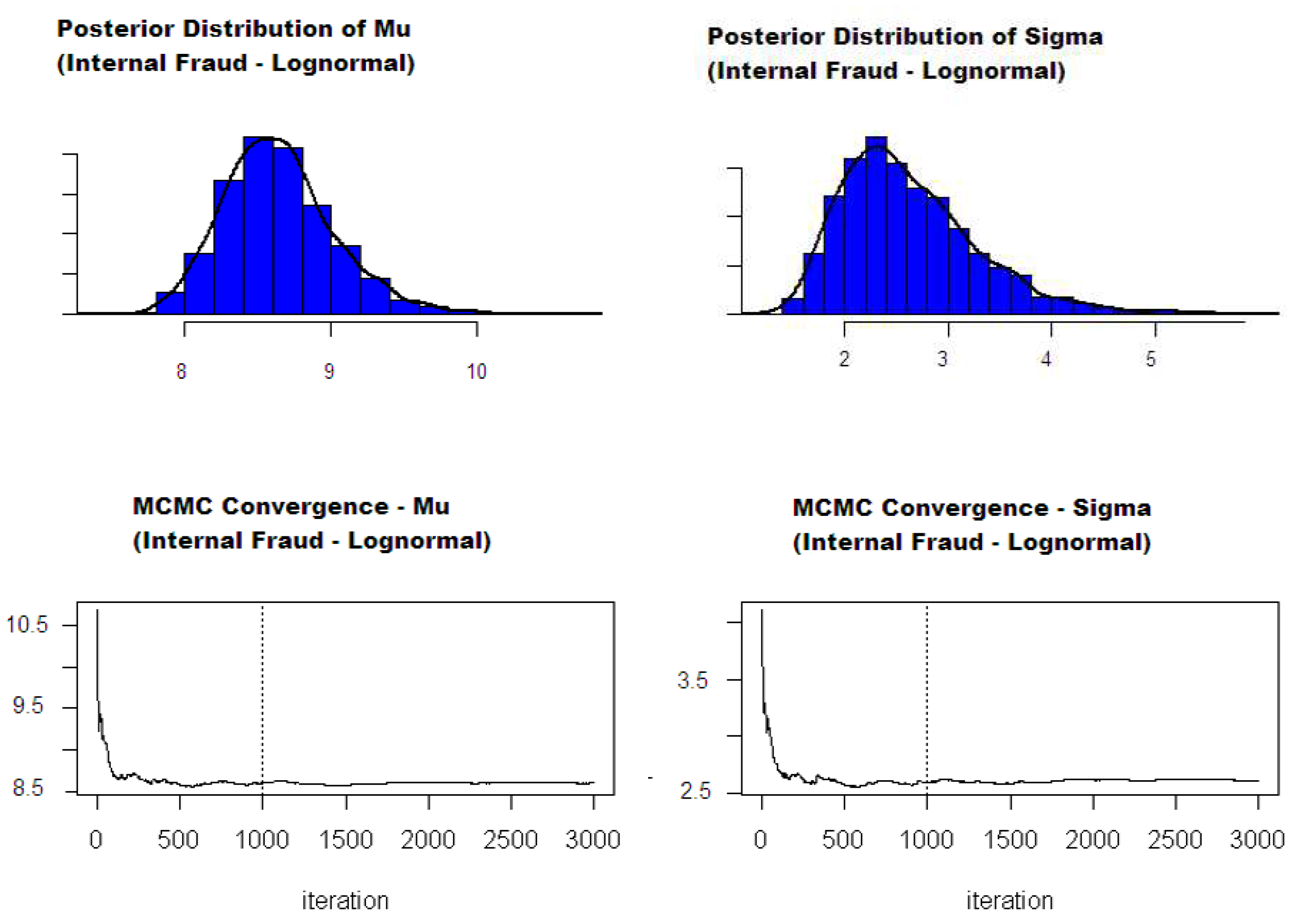
3.3. Estimation

To obtain the global severity parameters4 of the selected distributions, three different approaches may be carried out. These are listed below in the order of complexity.

• One can choose conjugate priors for the parameters in the first step of the Bayesian inference estimation. In this case, the (joint) distribution of the posterior parameters is directly known, and it is possible to sample directly from this distribution to recreate the marginal posterior distributions for each severity parameter. These may then be used to generate the posterior empirical densities required to compute a Bayesian point estimator of the parameters. The admissible estimators are the median, mean and mode of the posterior distribution. The mode (also called maximum a posteriori (MAP)) can be seen as the ’most probable estimator’ and ultimately coincides with the maximum likelihood estimator (Lehmann and Casella 1998). Despite having good asymptotic properties, finding the mode of an empirical distribution is not a trivial matter and often requires some additional techniques and hypotheses (e.g., smoothing). This paper, therefore, uses posterior means as point estimators. To the best of our knowledge, the only conjugate priors for continuous distributions were studied by Shevchenko (2011), for the Lognormal severity case. Conjugate approach requires some assumptions that may not be sustainable in practice, particularly for priors that are modelled with ’uncommon’ distributions (e.g., inverse-Chi-squared). This might lead to difficulties in the step known as ’elicitation’, i.e., calibrating the prior hyper-parameters from the chosen scenario values.
• Another solution is to release the conjugate prior assumption and use a Markov chain Monte Carlo approach in the first step to sample from the first posterior. One can then use a parametric or non-parametric method to compute the corresponding densities. This enables the posterior function to be evaluated (see Equation (6)). Maximising this function directly gives the MAP estimators of the severity parameters (see above). Even if this method is sufficient for computing values for the global parameters, it misses the purpose of the Bayesian inference, which is to provide distribution as a final result instead of a single value. In addition, it may also suffer from all the drawbacks that an optimisation algorithm may suffer (e.g., non-convex functions, sensitivity to starting values, etc.)
• The final alternative is to use a Markov chain Monte Carlo (MCMC) approach at each step of the aforementioned cascade Bayesian inference. This method is more challenging to implement but is the most powerful one, as it generates the entire distribution of the final severity parameters from which any credibility intervals and/or other statistics may be evaluated.

In this paper, the third alternative has been implemented using the Metropolis–Hastings algorithm. This allows sequential sampling from the two posterior distributions. This algorithm then enables us to build the distributions for the parameters contained in the $\varphi$ vector. However, these distributions are used as priors in the next step of the cascade and, as mentioned in the second point above, their densities are required from the sample obtained from the MCMC. Two solutions may be carried out—a parametric and a non-parametric one. The parametric solution requires fitting statistics to empirical distributions, which may introduce bias in the construction. To remain as close as possible to the empirical distributions that are generated and, therefore, to the data, a non-parametric approach based on a Kernel density estimation has been chosen. Using an Epanechnikov kernel and a cross-validation method to calibrate the bandwidth value, we can obtain the non-parametric density, representing the parameter’s distributions (Appendix A and Appendix B).

As a result, each of the different elements of the new posterior distribution has been built. The new prior densities in the second step result from the first posterior. The new likelihood function is informed by another data set, for instance, the internal loss data to guarantee an internal loss data-driven model.

Remark 1.

The innovation of this paper lies in the cascade Bayesian approach and its use to combine different sources of information. Consequently, little emphasis has been placed on our implementation of the MCMC with the Metropolis–Hastings algorithm, which is a known and widespread topic in literature. The interested reader could, for instance, refer to Gilks et al. (1996).

4. Results

The Cascade Bayesian approach enables the updating of the parameters of the distributions that are considered to model particular risk events.

Table 5. This table presents the standalone parameters estimated for each components. Internal fraud severities are modelled using a lognormal distribution, external fraud/payments using a Weibull and execution, delivery, and product management considering a mixture model combining a Lognormal distribution in the body and a generalized Pareto distribution in the tail. The first column presents the initial parameters estimated for the scenarios. ${\varphi }_1$ and ${\varphi }_2$ represent the severity parameters of the chosen distribution, i.e., (resp.) $\mu$ and $\sigma$ for the lognormal and shape and scale for the Weibull or GPD distribution. The second column shows the values obtained for the external data. The third column shows the parameters obtained for the internal data.

Label	Scenarios		External Data			Internal Data
	${\mathit{\varphi }}_1$	${\mathit{\varphi }}_2$	${\mathit{\varphi }}_1$	${\mathit{\varphi }}_2$	Size	${\mathit{\varphi }}_1$	${\mathit{\varphi }}_2$	Size
Internal Fraud	10.616031	2.024592	8.707405	2.693001	2956	9.347693	2.485755	665
(Global)—Lognormal
External Fraud	0.37642	4.6951 × 104	1.644924	5.4293 × 104	1085	0.292442	976.922586	1567
(Payments)—Weibull
Execution, Delivery,	0.4705893	1.5309 × 106	0.732526	1.1532 × 106	31126	0.82231	7.0388 × 105	3602
and Product Management
(Financial Instruments)—GPD

presents the parameters that are estimated, considering the different pieces of information used to build the loss distribution function (LDF), i.e., the parameters of the selected distributions. For instance, the lognormal, the Weibull and the generalized Pareto distribution are estimated on each of these pieces of information without considering the information introduced by the others. It results in a large variance in the parameters, which, once translated into financial values, may be inconsistent with the observations. For example, considering the lognormal distribution for internal fraud, the median is equal to 40,783.42, when considering only the scenarios, 6047.53, using the external data, and 11,472.33, considering the internal data. The parameter implied variance of the losses is also quite different across the different elements. The variation is similar for the Weibull distribution that models external fraud. It may be even worse in the case of the GPD, as the risk measures are extremely sensitive to the shape parameter.

Table 6. The table presents the evolution of the parameters obtained by carrying out the cascade Bayesian approach. Internal fraud severities are modelled using a Lognormal distribution, external fraud/payments using a Weibull and execution, delivery, and product management considering a mixture model combining a Lognormal distribution in the body and a generalized Pareto distribution in the tail. The first column presents the initial parameters estimated from the scenarios. ${\varphi }_1$ and ${\varphi }_2$ represent the severity parameters of the chosen distribution, i.e., (resp.) $\mu$ and $\sigma$ for the Lognormal and shape and scale for the Weibull or GPD distribution. The second column shows the values obtained after the first refinement, i.e., after the incorporation of the external data. The third column shows the final parameters following the second refinement, i.e., after the integration of the internal data. The figures in brackets represent a 95% Bayesian credible interval obtained from the final posterior distribution.

Label	Scenarios Severity from Priors		Intermediate Severity (Scenarios + External Data)		Final Severity (Scenarios + External Data + Internal Data)
	${\mathit{\varphi }}_1$	${\mathit{\varphi }}_2$	${\mathit{\varphi }}_1$	${\mathit{\varphi }}_2$	${\mathit{\varphi }}_1$	${\mathit{\varphi }}_2$
Internal Fraud (Global)—Lognormal	10.616031	2.024592	9.123964	2.539844	8.727855	2.684253
(95% Bayesian Credibility Interval)	-	-	-	-	[7.98176; 9.95824]	[1.23225; 4.42314]
External Fraud (Payments)—Weibull	0.3761	46942	0.38873	49,942	0.39910	46,622
(95% Bayesian Credibility Interval)	-	-	-	-	[0.23127; 0.50673]	[37,632; 58,981]
Execution, Delivery, and Product Management	0.4705893	1.5309 × 106	0.4452626	1.5109 × 106	0.6021	6.05 × 105
(Financial Instruments)—GPD
(95% Bayesian Credibility Interval)	-	-	-	-	[0.3313; 0.9089]	[4.52 × 105; 8.30 × 105]

shows the evolution of the parameters as they are updated with respect to the different pieces of information.

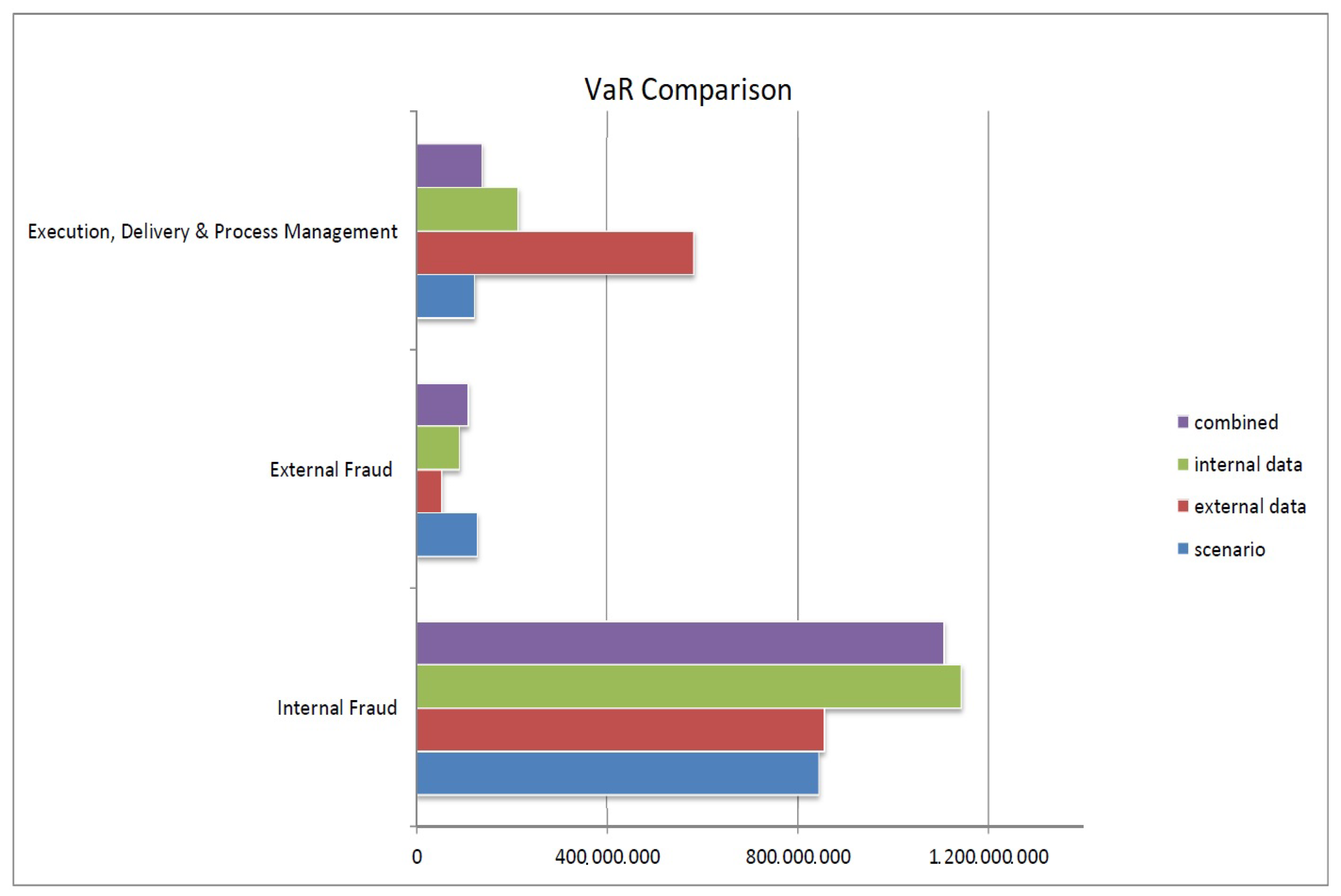
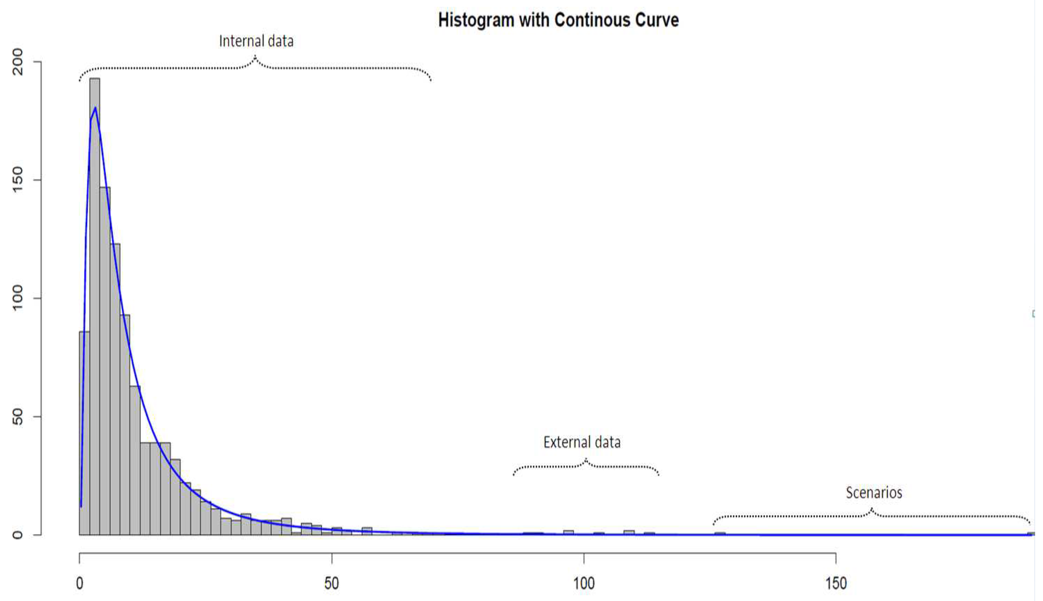
• Scenarios’ severity is derived from the calibration of the prior distributions with the scenario values. The theoretical means obtained from the calibrated priors provide scenario severity estimates.
• Intermediate severity refers to the estimation of the severity of the first obtained posterior, i.e., the mean of the posterior distribution obtained from scenario values updated with external loss data.
• Similarly, final severity represents the severity estimation of the second and last posterior distribution, which includes scenarios, external and internal loss data. A 95% Bayesian confidence interval (also known as a credible interval) derived from this final posterior distribution is also provided. It is worth noticing that this interval, which is formally defined as containing 95% of the distribution mass, is not unique and is chosen here as the narrowest possible interval. It is, therefore, not necessarily symmetric around the posterior mean estimator.

Implementation of the Cascade approach results in final parameters located within the range of values obtained from the different elements taken independently. As the dispersion of the information increases, the variance of the theoretical losses tends to increase, as does the theoretical kurtosis. For example, the evolution of the lognormal parameters is significant, as the introduction of data belonging to the body (Table 5, first line) tends to decrease the mean (the $\mu$ parameter is the mean of the log-transformed of the data). The parameters of the body part of the risk category for which a GPD is used to model the losses in the tail are provided in

Table 7. Body distribution (Lognormal) parameters for execution, delivery, and product management/financial instruments.

Event Type	$\mathit{\mu }$	$\mathit{\sigma }$
Execution, Delivery,	8.092849	1.882122
and Product Management
(Financial Instruments)—Lognormal body

. However, naturally, the dispersion increases, and, therefore, the variance tends to increase (the $\sigma$ parameter is a representation of the standard deviation of the log-transform of the data) (Table 6, first line). The impact of the severity on frequency is given in

Table 8. Frequency distribution parameters used in the capital charge calculations. GDP: generalized Pareto distribution.

Event Type	Initial$\mathit{\lambda }$	Corrected$\mathit{\lambda }$
Internal Fraud	133	261.5885
(Global)—Lognormal
External Fraud	313.4	485.0353
(Payments)—Weibull
Event Type	Initial$\mathit{\lambda }$body	Initial$\mathit{\lambda }$tail	Initial Global$\mathit{\lambda }$	Corrected Global$\mathit{\lambda }$
Execution, Delivery,	144.08	9.2	153.28	1882.327
and Product Management
(Financial Instruments)—GPD

. The conditional frequencies naturally increase with respect to the severity distributions.

It also results in conservative capital charges, considering the VaR (Appendix D) obtained from the different elements taken independently, as it tends to be a weighted average of the VaR obtained from each part. The weights are automatically evaluated during the cascade and directly related to the quantity and the quality of information integrated (

Table 9. This table presents the stand alone value-at-risk (VaR) for each of the three components, as well as the VaR and the expected shortfall (ES) computed by combining the three elements with cascade Bayesian integration for each of the three different event types. Internal fraud severities are modelled using a Lognormal distribution, external fraud/payments using a Weibull and execution, delivery, and product management considering a mixture model combining a lognormal distribution in the body and a generalized Pareto distribution in the tail. The parameters of the distributions used to compute these values are shown in Table 5 and Table 6.

Label	Scenarios	External Data	Internal Data	Combination
	VaR	VaR	VaR	VaR	ES
Internal Fraud	843,445,037	855,464,158	1,143,579,396	1,106,692,211	2,470,332,812
(Global)
External Fraud Payments	128,243,367	13,664,057	3,945,116	119,637,592	126,935,364
(Payments)
Execution, Delivery, and Product Management	122,544,708	583,519,888	137,456,938	213,982,300	281,157,384
(Financial Instruments)

).

Practically, implementing the solution presented in this paper, the following remarks should be carefully considered:

Remark 2.

The scenarios are defined by the bank. As mentioned previously, eventually all elements have to be combined, though internal data and scenarios are collected by the bank, external data are not. Both external data and scenarios are belonging to the domain of ’observable’ losses and therefore are belonging to the domain of what may happen (either in magnitude, in frequency or in type of incidents). Consequently, in the Bayesian inference philosophy, these should inform the prior functions. On the other hand, internal data are belonging to the domain of what had happened and therefore these should inform what we referred to as the ’likelihood component’.

Remark 3.

In our case, the scenarios are representing events located far in the right tail and have been collected given specific percentiles; therefore, if the internal data are not numerous enough, combining them directly in the posterior may lead to very large capital charges. On the contrary, if the internal data set is very large, the scenarios would have a very limited impact on the capital charge.

Remark 4.

In this paper, we started form the tail, i.e., the most conservative part of the distribution, using the few largest events to inform the prior. Then, external data are integrated as these are closer to the scenarios. The objective is to avoid a gap too large between scenarios and internal data. Indeed, we observed that a large gap between the element informing the prior and the elements informing the ’likelihood component’ may prevent the MCMC algorithm from converging.

Remark 5.

It is noteworthy to mention that some prior distributions have been chosen to constrain the range of parameter’s values. For instance, considering the generalised Pareto distribution, the use of the beta distribution to characterise the shape parameter is justified by the fact that this parameter would mechanically lie between 0 and 1 and therefore this approach would prevent infinite mean models.

As a final step, these results may be illustrated for the whole Bayesian cascade estimation in the simple lognormal case. Figure 2 shows the final posterior distribution obtained for $\mu$ and $\sigma$. This is used to derive the 95% Bayesian credible interval given in Table 6. We also show the results of the convergence of the posterior mean as a function of the number of MCMC iterations for ($\mu$ and $\sigma$). One can see that the values stabilise after 100 to 500 iterations in this example. In the general case, we chose to sample 3000 values and discard the first 1000 MCMC generated values (burn-in period) to ensure the stability of our estimates.

5. Conclusions

This paper presents an intuitive approach to building the loss distribution function using the Bayesian inference framework and combining the different regulatory components. This approach overcomes the problem related to the non-homogeneity of the data.

This approach enables the controlled integration of the different elements through the Bayesian inference. The prior functions have the same role as the penalisation functions on the parameters and, therefore, behave as constraints during the estimation procedure. This results in capital charges being driven by internal data (as shown in Figure 3), which are not dramatically influenced by external data or extreme scenarios.

Hence, with our approach, the capital requirement calculation is inherently related to the risk profile of the target financial institution and, therefore, provides the senior management with greater assurance of the validity of the results.

As presented in the previous section of this paper, best practices, i.e., practices approved by the regulator for AMA capital calculations, are highly heterogeneous, therefore it is necessary to reinforce the fact that there is no panacea, there are only methodologies or modelling strategies more appropriate than others in particular situation. As such, this methodology can be really interesting in an environment similar to the one presented in this paper.

The next step is to evaluate the financial institutions’ global operational risk capital requirement would involve the construction of the multivariate distribution function, linking the different loss distributions that characterise the various event types through a copula. In this case, the approach developed by Guegan and Hassani (2013a) may be of interest.

References

- Álvarez, Gene. 2001. Operational Risk Quantification Mathematical Solutions for Analyzing Loss Data. Available online: https://www.bis.org/bcbs/ca/galva.pdf (accessed on 26 April 2018).
- Bayes, Thomas. 1763. An Essay towards Solving a Problem in the Doctrine of Chances. By the Late Rev. Mr. Bayes, F. R. S. Communicated by Mr. Price, in a Letter to John Canton, A. M. F. R. S. Philosophical Transactions (1683–1775) 53: 370–418. [Google Scholar] [CrossRef]
- BCBS. 2001. Working Paper on the Regulatory Treatment of Operational Risk. Basel: Bank for International Settlements. [Google Scholar]
- BCBS. 2010. Basel III: A Global Regulatory Framework for More Resilient Banks and Banking Systems. Basel: Bank for International Settlements. [Google Scholar]
- Berger, James O. 1985. Statistical Decision Theory and Bayesian Analysis. New York: Springer. [Google Scholar]
- Böcker, Klaus, and Claudia Klüppelberg. 2010. Operational VaR: A Closed-Form Approximation. Risk 18: 90–93. [Google Scholar]
- Bowman, Adrian W. 1984. An alternative method of cross-validation for the smoothing of density estimates. Biometrika 71: 353–60. [Google Scholar] [CrossRef]
- Box, George E. P., and George C. Tiao. 1992. Bayesian Inference in Statistical Analysis. New York, Chichester and Brisbane: Wiley Classics Library, JohnWiley & Sons. [Google Scholar]
- Chernobai, Anna S., Svetlozar T. Rachev, and Frank J. Fabozzi. 2007. Operational Risk: A Guide to Basel II Capital Requirements, Models, and Analysis. New York: John Wiley & Sons. [Google Scholar]
- Cowell, Robert G., Richard J. Verrall, and Y. K. Yoon. 2007. Modeling operational risk with bayesian networks. Journal of Risk and Insurance 74: 795–827. [Google Scholar] [CrossRef]
- Cruz, Marcelo G. 2004. Operational Risk Modelling and Analysis. London: Risk Books. [Google Scholar]
- Cruz, Marcelo G., Gareth W. Peters, and Pavel V. Shevchenko. 2014. Fundamental Aspects of Operational Risk and Insurance Analytics: A Handbook of Operational Risk. Hoboken: John Wiley & Sons. [Google Scholar]
- Frachot, Antoine, Pierre Georges, and Thierry Roncalli. 2001. Loss Distribution Approach for Operational Risk. Working paper. Paris: GRO, Crédit Lyonnais. [Google Scholar]
- Gilks, Walter R., Sylvia Richardson, and David Spiegelhalter. 1996. Markov Chain Monte Carlo in Practice. London: Chapman & Hall/CRC. [Google Scholar]
- Guegan, Dominique, and Bertrand K. Hassani. 2013. Multivariate vars for operational risk capital computation: A vine structure approach. International Journal of Risk Assessment and Management 17: 148–70. [Google Scholar] [CrossRef]
- Guégan, Dominique, and Bertrand Hassani. 2013. Using a time series approach to correct serial correlation in operational risk capital calculation. The Journal of Operational Risk 8: 31. [Google Scholar] [CrossRef]
- Guégan, Dominique, and Bertrand Hassani. 2014. A mathematical resurgence of risk management: An extreme modeling of expert opinions. Frontiers in Finance & Economics 11: 25–45. [Google Scholar]
- Guégan, Dominique, Bertrand K. Hassani, and Cédric Naud. 2011. An efficient threshold choice for the computation of operational risk capital. The Journal of Operational Risk 6: 3–19. [Google Scholar] [CrossRef]
- Hassani, Bertrand, and Bertrand K. Hassani. 2016. Scenario Analysis in Risk Management. Cham: Springer. [Google Scholar]
- Lehmann, Erich L., and George Casella. 1998. Theory of Point Estimation, 2nd ed. Berlin: Springer. [Google Scholar]
- Leone, Paola, and Pasqualina Porretta. 2018. Operational risk management: Regulatory framework and operational impact. In Measuring and Managing Operational Risk. Cham: Palgrave Macmillan, pp. 25–93. [Google Scholar]
- Mizgier, Kamil J., and Maximilian Wimmer. 2018. Incorporating single and multiple losses in operational risk: A multi-period perspective. Journal of the Operational Research Society 69: 358–71. [Google Scholar] [CrossRef]
- Parent, Eric, and Jacques Bernier. 2007. Le Raisonnement Bayésien, Modelisation Et Inférence. Paris: Springer. [Google Scholar]
- Peters, Gareth William, and Scott Sisson. 2006. Bayesian inference, Monte Carlo sampling and operational risk. Journal of Operational Risk 1. [Google Scholar] [CrossRef]
- Peters, Gareth W., and Pavel V. Shevchenko. 2015. Advances in Heavy Tailed Risk Modeling: A Handbook of Operational Risk. Hoboken: John Wiley & Sons. [Google Scholar]
- Rudemo, Mats. 1982. Empirical choice of histograms and kernel density estimators. Scandinavian Journal of Statistics 9: 65–78. [Google Scholar]
- Shevchenko, Pavel V. 2011. Modelling Operational Risk Using Bayesian Inference. Berlin: Springer. [Google Scholar]
- Valdés, Rosa María Arnaldo, V. Fernando Gómez Comendador, Luis Perez Sanz, and Alvaro Rodriguez Sanz. 2018. Prediction of aircraft safety incidents using Bayesian inference and hierarchical structures. Safety Science 104: 216–30. [Google Scholar] [CrossRef]