The Italian Pension Gap: A Stochastic Optimal Control Approach

Abstract

We study the gap between the state pension provided by the Italian pension system pre-Dini reform and post-Dini reform. The goal is to fill the gap between the old and the new pension by joining a defined contribution pension scheme and adopting an optimal investment strategy that is target-based. We find that it is possible to cover, at least partially, this gap with the additional income of the pension scheme, especially in the presence of late retirement and in the presence of stagnant careers. Workers with dynamic careers and workers who retire early are those who are most penalised by the reform. Results are intuitive and in line with previous studies on the subject.

1. Introduction

During the last few decades, several countries across the world have faced the ageing population problem. It is well known that the ageing of the population threatens the sustainability of Pay-As-You-Go (PAYG) pension systems, which are essentially based on a sufficiently high ratio of workers to pensioners. To tackle this issue, many governments have introduced new reforms that lead to deep changes into the pension systems.

In particular, in Italy, the Dini reform (introduced in 1995) instituted a completely different pension system for new classes of workers. Before the reform, the public pension was provided through a defined benefit salary-related system. Namely, the pension provided was simply a service-based percentage of the last salary of the worker. After the reform, the public pension is provided through a contribution-based system, the so called notional defined contribution (NDC) system1, where the worker contributes by himself to build his pension.

This remarkable change generated two different classes of workers, the pre-reform workers and the post-reform workers, and led to a pension gap between their corresponding pension rates and replacement ratios. According to Borella and Coda Moscarola (2010), the common perception is that, while the pre-reform system provided an adequate level of pension, the post-reform system will not. To be more specific, Borella and Coda Moscarola (2010) measure the drop in adequacy of the new system, by projecting future replacement ratios (the replacement ratio is the ratio between the first rate of pension and the last salary) and comparing them with replacement ratios obtained with the old system. Unsurprisingly, they find that passing from the old to the new system the replacement ratio decreases. In particular, the median replacement ratio for private employees ranges between 64% and 67% before the reform, while it is about 54% after the reform; for self-employees it ranges between 67% and 72% before the reform, while it ranges between 38% and $41\%$ after the reform.

The aim of this paper is to illustrate a possible way to fill this pension gap investing optimally in a defined contribution (DC) pension fund during working life. In order to achieve this goal, a stochastic optimal control problem with suitable annual targets is solved. We consider two different salary growths to represent two different classes of workers: a linear salary growth (blue-collar workers) and an exponential salary growth (white-collar workers).

A numerical section illustrates the practical application of the model. Our results are in line with previous results on the comparison between the old pre-reform Italian pension and the new post-reform one, see Borella and Coda Moscarola (2006, 2010). We find that the gap between salary-related pension and contribution-based pension is larger for workers with dynamic careers than for workers with stagnant careers. This result is consistent with Bucciol et al. (2017), who find that in Italy the presence of the NDC pension system reduces inequality in disposable income. A slow salary increase associated to late retirement can produce a new pension that is almost equal to (or even exceeds) the old pension. Expectedly, the gap is easier to cover in the case of late retirement, and vice versa. Interestingly, the gap increases when the rate of growth of salary increases.

The reminder of the paper is as follows. In Section 2, we introduce the milestones of the Italian pension system and the consequences of the Dini reform. In Section 3, we build the model and the corresponding stochastic optimal control problem. In Section 4, we derive the closed-form solutions to the problem for the two different salary growths considered. In Section 5, we carry out some simulations in order to test the model and show the behaviour of the optimal investment strategy and the optimal fund growth in a base case scenario. In Section 6, we perform a sensitivity analysis of the pension distribution with respect to retirement age. In Section 7, we investigate the break-even points that render the “new” pension equal to the “old” pension. Section 8 concludes.

2. The Italian Pension Provision

The Italian pension system has been modified through a series of legislative measures taken by different governments during the 1990s. We only consider the Dini reform, which is sufficient to understand the following model.

The Dini reform (law 335, 1995) has changed the system for the calculation of the pension from a salary-based system to a contribution-related system. The workers shifted from one system to the other depending on the contributions paid at the end of 1995. Therefore, three different situations were created:

• The workers with at least eighteen years of contributions on 31 December 1995 remained under the salary-related system and therefore were not touched by the reform.
• The workers with less than eighteen years of contributions on 31 December 1995 were subject to a mixed method.
• The workers who were first employed after 31 December 1995 are subject to the contribution-based system.

In this paper, we compare the method of calculation for the public pension, before the Dini reform, with the “new” method of calculating public pension, after the reform.

The formula for the pension rate $P_o$ before the Dini reform was

$$P_o=0.02·T·S\left(T\right)$$

(1)

where $S\left(T\right)$ is the final salary, and T indicates the number of past working years. In the following, we shall call the pension rate in Equation (1) the “old pension.” The old pension is a percentage of the product of the last salary by the years of service, and the related net replacement ratio—which is the ratio between the first pension rate received after retirement and the last salary perceived before retirement—is given by

$${\mathsf{\Pi }}_o=\frac{P_o}{S\left(T\right)}=0.02·T.$$

(2)

In contrast, the new formula for the pension rate $P_n$ is described by

$$P_n=\beta ·c·\sum _{t=0}^{T-1}S\left(t\right){(1+w)}^{T-t}$$

(3)

where

• w is the mean real GDP (Gross Domestic Product) increase.
• T indicates the number of past working years (for instance $T=20,30,35,40$).
• c is the contribution percentage for the calculation of the pension rate (supposed to be constant during the whole working life and, for the employees, set by law to 33%).
• $\beta$ is the conversion coefficient between a lump sum and the annuity rate, and its choice should reflect actuarial fairness. If it does, then $\beta =1/{\ddot{a}}_x$, where ${\ddot{a}}_x$ is the single premium of a lifetime annuity issued to a policyholder aged x, i.e.,

  $${\ddot{a}}_x=\sum _{n=1}^{\omega -x}{}_n{p}_x·v^n$$

  (4)

  where $\omega$ is the extreme age, $v=1/(1+r)$ is the annual discount factor, and ${}_n{p}_x$ is the survival probability from age x to age $x+n$.

In the following, we shall call the pension rate of Equation (3) the “new pension.” Compared to the old pension, the new pension is given by a complicated formula and depends not only on all salaries but also on other parameters. Its related net replacement ratio is

$${\mathsf{\Pi }}_n=\frac{P_n}{S\left(T\right)}.$$

(5)

3. The Optimization Problem

The main idea of this paper is the following.

We assume that the worker was firstly employed after 31 December 1995 and will receive the new pension (Equation (3)) from the first pillar (i.e., the public pension), but he wants to integrate it with additional income from the second pillar (i.e., the private pension funds) to obtain a pension rate that is as close as possible to the one that he would have obtained with the old pension rule (1). Since the Dini reform, and apart from a few exceptions accessible only by self-employed (not considered in this paper), pension funds in Italy are defined contribution (DC) and not defined benefit (DB). This means that the contribution to be paid into the fund is fixed a priori in the scheme’s rules and the benefit obtained at retirement depends on the investment performance of the fund in the accumulation period.

We assume that at time 0 the worker joins a DC pension scheme and has control over the investment strategy to be adopted on the time horizon $[0,T]$, where T is the retirement time. The financial market consists of two assets, a riskless asset with price $B={\left\{B\left(t\right)\right\}}_{t\ge 0}$ and a risky asset with price $Z={\left\{Z\left(t\right)\right\}}_{t\ge 0}$, whose dynamics are described by

$$dB\left(t\right)=rB\left(t\right)dt$$

(6)

$$dZ\left(t\right)=\mu Z\left(t\right)dt+\sigma Z\left(t\right)dW\left(t\right)$$

(7)

where r is a constant rate of interest, and ${\left\{W\left(t\right)\right\}}_{t\ge 0}$ is a standard Brownian motion defined and adapted on a complete filtered probability space $(\mathsf{\Omega },\mathcal{F},{\left\{{\mathcal{F}}_t\right\}}_{t\ge 0},\mathbb{P})$. We assume that the contribution $c\left(t\right)$ paid into the fund at time t is a fixed proportion of the salary of the member

$$c\left(t\right)=kS\left(t\right),t\in [0,T]$$

(8)

where $k\in (0,1)$ and $S\left(t\right)$ is the salary of the member at time t. Finally, the proportion of portfolio invested into the risky asset at time $t\in [0,T]$ is $y\left(t\right)$. Hence, the dynamics of the wealth are described by the the following stochastic differential equation:

$$\left\{\begin{array}{c}dX\left(t\right)=\left\{\right[(\mu -r)y\left(t\right)+r\left]X\right(t)+c(t\left)\right\}dt+\sigma y\left(t\right)X\left(t\right)dW\left(t\right)\hfill \\ X\left(0\right)=x_0\hfill \end{array}\right.$$

(9)

where $x_0\ge 0$ is the initial wealth paid into the fund (it can also be a transfer value from another pension fund). Because the aim of the worker is to reach a pension rate that is as close as possible to that of the salary-related method, we assume that there exist annual targets ${\left\{F\left(t\right)\right\}}_{t=0,1,2,\cdots ,T}$ that he wants to achieve, and that his preferences are described by the loss suffered when the targets are not met. Thus, we introduce the following quadratic loss (or disutility) function

$$L(t,X\left(t\right))={(F\left(t\right)-X\left(t\right))}^2,t\in [0,T].$$

(10)

Remark 1.

The use of a quadratic loss is very common in the context of pension funds. Examples include Boulier et al. (1995, 1996), Cairns (2000), and Gerrard et al. (2004, 2006, 2012). Moreover, Vigna (2014) and Menoncin and Vigna (2017) analysed and discussed the link between “utility-based” and “target-based” approaches. From a theoretical point of view, the quadratic loss function penalizes any deviations above the target, and this can be considered a drawback to the model. However, the choice of trying to achieve a target and no more than this has the effect of a natural limitation on the overall risk of the portfolio: once the desired target is reached, there is no reason for further exposure to risk and the surplus therefore becomes undesirable. This is in accordance with the fact that the mean–variance approach to portfolio selection has been shown to be equivalent to the minimization of a quadratic loss function: see the seminal papers by Zhou and Li (2000), Li and Ng (2000), and, in the context of DC pension schemes, Vigna (2014). The idea that people act by following subjective targets is also accepted in the decision theory literature. For instance, Kahneman and Tversky (1979) support the use of targets in the cost function, and Bordley and LiCalzi (2000) support the target-based approach in decision-making under uncertainty.

We now need to define the targets. Recalling that the worker’s goal is to reach the old pension pre-Dini reform, we set as final target $F\left(T\right)$ the amount that the retiree aged x should pay to an insurance company in order to fill the gap between the previous pension rate and the current one, i.e.,

$$F\left(T\right)=(P_o-P_n){\ddot{a}}_x$$

(11)

where ${\ddot{a}}_x$ is the price of the annuity given by Equation (4) to a retiree aged x, $P_o$ is given by Equation (1), and $P_n$ is the continuous formulation of Equation (3), which means

$$P_n=\beta c{\int }_0^{T}S\left(t\right)e^{w(T-t)}dt.$$

(12)

The interim targets $F\left(t\right)$ for $t\in [0,T)$ are set to be the compounded value of the fund plus contributions using the interest rate $r^{\ast }$ that matches a continuity condition between interim targets and the final target, i.e.,

$$F\left(t\right)=x_0{e}^{r^{\ast }t}+{\int }_0^{t}c\left(s\right)e^{r^{\ast }(t-s)}ds$$

(13)

with $r^{\ast }$ such that2

$$\underset{t\to T^{-}}{lim}F\left(t\right)=F\left(T\right).$$

(14)

The worker’s goal is to minimize the conditional expected losses that can be experienced from the fund until retirement, i.e., the goal is to minimize the following expectation:

$${\mathbb{E}}_{0,x_0}\left[{\int }_0^T{e}^{-\rho s}L(s,X\left(s\right))ds+e^{-\rho T}L(T,X\left(T\right))\right]$$

(15)

where $\rho >0$ is the (subjective) intertemporal discount factor.

As usual in optimization problems in DC pension schemes, the contribution rate is not a control variable, and the only control variable for the worker is the share of portfolio $y\left(t\right)$ to be invested into the risky asset at time $t\in [0,T]$. To formulate the optimization problem, we define the performance criterion at time t with wealth x, i.e.,

$$J_{t,x}\left(y(·)\right)={\mathbb{E}}_{t,x}\left[{\int }_t^T{e}^{-\rho s}L(s,X\left(s\right))ds+e^{-\rho T}L(T,X\left(T\right))\right],$$

(16)

and the admissible strategies.

Definition 1.

An investment strategy $y(·)$ is said to be admissible if $y(·)\in L_{\mathcal{F}}^2(0,T;\mathbb{R})$.

The minimization problem, then, becomes

$$\mathrm{Minimize}{J}_{0,x_0}\left(y(·)\right)$$

(17)

over the set of admissible strategies.

4. Solution

In order to solve the optimization problem (17), the value function is defined as

$$V(t,x)=\underset{y(·)}{inf}{J}_{t,x}\left(y(·)\right),\forall (t,x)\in U=[0,T]\times (-\infty ,+\infty ).$$

(18)

Remark 2.

In this work, we neither set boundaries on the values that the fund $X(·)$ can assume, nor set boundaries on the share $y\left(t\right)$ to be invested in the risky asset. The existence of a minimum finite bound on $X\left(t\right)$ would be desirable, as well as proper boundaries on the investment strategy. The former would be intended to protect the retiree from outliving his asset and not being able to buy a minimum level of pension at time T, the latter to comply with the usual forbiddance of short-selling and borrowing. However, adding restrictions to the state variable and the control variable means adding boundary conditions to the problem, and this makes it extremely hard (and often impossible) to solve analytically. Among the few works that treat optimization problems with restrictions in DC pension schemes, see Di Giacinto et al. (2011, 2014).

We write the Hamilton-Jacobi-Bellman (HJB) equation:

$$\underset{y\in \mathbb{R}}{inf}[e^{-\rho t}L(t,x)+{\mathcal{L}}^{y}V(t,x)]=0,\forall (t,x)\in U$$

(19)

$$V(T,x)=e^{-\rho T}L(T,x),\forall x\in \mathbb{R}$$

(20)

where

$${\mathcal{L}}^{u}f(t,x)=\frac{\partial }{\partial t}f(t,x)+b(t,x,u)\frac{\partial }{\partial x}f(t,x)+\frac{1}{2}{\sigma }^2(t,x,u)\frac{{\partial }^2}{\partial x^2}f(t,x)$$

(21)

is the infinitesimal operator, and the functions $b(·)$ and $\sigma (·)$ are the drift and diffusion terms of the process $X={\left\{X\left(t\right)\right\}}_{t\ge 0}$, defined by Equation (9).

Substituting into Equation (19), we obtain $\forall (t,x)\in U$:

$$\underset{y\in \mathbb{R}}{inf}\left\{e^{-\rho t}{(F\left(t\right)-x)}^2+\frac{\partial V}{\partial t}+[x(y(\mu -r)+r)+c\left(t\right)]\frac{\partial V}{\partial x}+\frac{1}{2}{x}^2{y}^2{\sigma }^2\frac{{\partial }^{2}V}{\partial x^2}\right\}=0,$$

(22)

with the boundary condition

$$V(T,x)=e^{-\rho T}L(T,x).$$

(23)

For simpler notation, let us define

$$\psi (t,x,y)=e^{-\rho t}{(F\left(t\right)-x)}^2+\frac{\partial V}{\partial t}+[x(y(\mu -r)+r)+c\left(t\right)]\frac{\partial V}{\partial x}+\frac{1}{2}{x}^2{y}^2{\sigma }^2\frac{{\partial }^{2}V}{\partial x^2}.$$

(24)

Thus, Equation (22) becomes

$$\underset{y\in \mathbb{R}}{inf}\psi (t,x,y)=0\Rightarrow \psi (t,x,y^{\ast })=0.$$

(25)

The first and second order conditions are

$${\psi }_y(t,x,y^{\ast })=0$$

(26)

$${\psi }_{yy}(t,x,y^{\ast })>0.$$

(27)

Therefore, Equation (26) becomes

$$x(\mu -r)\frac{\partial V}{\partial x}+x^2{y}^{\ast }{\sigma }^2\frac{{\partial }^{2}V}{\partial x^2}=0,$$

(28)

so that

$$y^{\ast }=-\frac{\mu -r}{\sigma }\frac{1}{x\sigma }\frac{V_x}{V_{xx}}.$$

(29)

Moreover, the condition of Equation (27) is satisfied if and only if

$$x^2{\sigma }^2\frac{{\partial }^{2}V}{\partial x^2}>0\iff \frac{{\partial }^{2}V}{\partial x^2}>0.$$

(30)

We will show later that this condition is actually satisfied, so that the solution is a minimum.

By substituting Equation (29) into Equation (25), we obtain the non-linear partial differential equation

$$e^{-\rho t}{(F\left(t\right)-x)}^2+V_t+[rx+c\left(t\right)]V_x-\frac{1}{2}{\left(\frac{\mu -r}{\sigma }\right)}^2\frac{V_x^2}{V_{xx}}=0.$$

(31)

We guess a solution of the form

$$V(t,x)=e^{-\rho t}[\alpha \left(t\right)x^2+\beta \left(t\right)x+\gamma \left(t\right)].$$

(32)

From the boundary condition, expressed in Equation (23), we obtain

$$e^{-\rho T}{(F\left(T\right)-x)}^2=e^{-\rho T}[\alpha \left(T\right)x^2+\beta \left(T\right)x+\gamma \left(T\right)],\forall x\in (-\infty ,+\infty ),$$

(33)

so that

$$\alpha \left(T\right)=1,\beta \left(T\right)=-2F\left(T\right),\gamma \left(T\right)={\left[F\left(T\right)\right]}^2.$$

(34)

The partial derivatives of V are

$$V_t(t,x)=-\rho e^{-\rho t}[\alpha \left(t\right)x^2+\beta \left(t\right)x+\gamma \left(t\right)]+e^{-\rho t}[{\alpha }^{\prime }\left(t\right)x^2+{\beta }^{\prime }\left(t\right)x+{\gamma }^{\prime }\left(t\right)]$$

(35)

$$V_x(t,x)=e^{-\rho t}[2\alpha \left(t\right)x+\beta \left(t\right)],V_{xx}(t,x)=2e^{-\rho t}\alpha \left(t\right),$$

(36)

and substituting them into Equation (29), we derive the optimal investment strategy at time t with wealth x, i.e.,

$$y^{\ast }(t,x)=-\frac{\mu -r}{\sigma }\frac{1}{x\sigma }\left(x+\frac{\beta \left(t\right)}{2\alpha \left(t\right)}\right).$$

(37)

Substituting the partial derivatives of $V(·,·)$ into Equation (31), we have

$$\begin{array}{c}[1-\rho \alpha \left(t\right)+{\alpha }^{\prime }\left(t\right)+2r\alpha \left(t\right)-{\lambda }^2\alpha \left(t\right)]x^2+[-2F\left(t\right)-\rho \beta \left(t\right)+{\beta }^{\prime }\left(t\right)+r\beta \left(t\right)+\\ +2\alpha \left(t\right)c\left(t\right)-{\lambda }^2\beta \left(t\right)]x+\left[F{\left(t\right)}^2-\rho \gamma \left(t\right)+{\gamma }^{\prime }\left(t\right)+c\left(t\right)\beta \left(t\right)-{\lambda }^2\frac{\beta {\left(t\right)}^2}{4\alpha \left(t\right)}\right]=0\end{array}$$

(38)

where $\lambda =(\mu -r)/\sigma$ is the Sharpe ratio of the risky asset.

Since Equation (38) must hold $\forall (t,x)\in U$, we derive the following system of ordinary differential equations

$$\left\{\begin{array}{c}{\alpha }^{\prime }\left(t\right)=[\rho +{\lambda }^2-2r]\alpha \left(t\right)-1=a\alpha \left(t\right)-1\hfill \\ {\beta }^{\prime }\left(t\right)=[\rho +{\lambda }^2-r]\beta \left(t\right)+2F\left(t\right)-2c\left(t\right)\alpha \left(t\right)=\tilde{a}\beta \left(t\right)+2F\left(t\right)-2c\left(t\right)\alpha \left(t\right)\hfill \\ {\gamma }^{\prime }\left(t\right)=\rho \gamma \left(t\right)-F{\left(t\right)}^2-c\left(t\right)\beta \left(t\right)+{\lambda }^2\frac{\beta {\left(t\right)}^2}{4\alpha \left(t\right)}\hfill \end{array}\right.$$

(39)

where we have defined $a=\rho +{\lambda }^2-2r$, $\tilde{a}=a+r$, and with the boundary conditions expressed in Equation (34).

4.1 Solution to the Problem with Two Different Salary Evolutions

Two different salaries are compared. A linear salary,

$$S_l\left(t\right)=S_0(1+g_{l}t),t\in [0,T],$$

(40)

and an exponential salary,

$$S_e\left(t\right)=S_0{e}^{g_{e}t},t\in [0,T]$$

(41)

where $S_0$ is the initial salary, and $g_i$ ($i=l,e$) is the mean real salary increase.

The contribution in the two cases is

$$c_i\left(t\right)=k_i{S}_i\left(t\right),t\in [0,T],i=l,e.$$

(42)

Remark 3.

We have selected two simple models for salary growth for analytical tractability and the aim of providing closed-form solutions for the optimal investment strategy.3 While the exponential salary growth is standard in the actuarial literature on DC pension schemes (see e.g. Battocchio and Menoncin (2004), Boulier et al. (2001), Cairns et al. (2006), Deelstra et al. (2003), Menoncin and Vigna (2017)), a linear salary growth seems also suitable to describe the salary growth over age, see Figure 3 in Jessen et al. (2018) and Figures 1,2 in Borella and Coda Moscarola (2015) (those figures report a linear increase with age, with a downward trend prior to retirement). The two different salary growths may represent two different categories of workers, the exponential growth associated with white-collar workers with dynamic salary increases, the linear salary increase associated with blue-collar workers with smooth salary increases. The distinct $k^{\prime }s$ reflect the assumption that the savings capacity of white-collar workers is higher than the savings capacity of blue-collar workers. Finally, notice that in our model we have not introduced any factor that reflects heterogeneity of workers (e.g. gender, education level, etc). However, as illustrated in Bucciol et al. (2017), a more accurate analysis of heterogeneity may affect the salary levels of the workers.

Therefore, there are also two different families of targets.

For the linear salary case (for notational convenience, in the following, we will write g and k in the place of $g_l$ and $k_l$):

$$\begin{array}{cc}\hfill F_l\left(t\right)& =x_0{e}^{r^{\ast }t}+{\int }_0^{t}k{S}_0(1+gs)e^{r^{\ast }(t-s)}ds\hfill \\ & =\left[x_0+\frac{k{S}_0}{r^{\ast }}+\frac{kg{S}_0}{{\left(r^{\ast }\right)}^2}\right]e^{r^{\ast }t}-\frac{kg{S}_0}{r^{\ast }}t-\frac{k{S}_0}{r^{\ast }}\left[1+\frac{g}{r^{\ast }}\right]\hfill \end{array}$$

(43)

$$F_l\left(T\right)=({\mathsf{\Pi }}_o-{\mathsf{\Pi }}_n^l)S_l\left(T\right){\ddot{a}}_x$$

(44)

where ${\mathsf{\Pi }}_n^l$ is the net replacement ratio for the new public pension with linear salary.

For the exponential salary case (for notational convenience, in the following, we will write g and k in the place of $g_e$ and $k_e$):

$$F_e\left(t\right)=x_0{e}^{r^{\ast }t}+{\int }_0^{t}k{S}_0{e}^{gs}{e}^{r^{\ast }(t-s)}ds=\left[x_0-\frac{k{S}_0}{g-r^{\ast }}\right]e^{r^{\ast }t}+\frac{k{S}_0}{g-r^{\ast }}{e}^{gt}$$

(45)

$$F_e\left(T\right)=({\mathsf{\Pi }}_o-{\mathsf{\Pi }}_n^e)S_e\left(T\right){\ddot{a}}_x$$

(46)

where ${\mathsf{\Pi }}_n^e$ is the net replacement ratio for the new public pension with exponential salary.

Solving the system expressed in Equation (39) in both cases, we find the following solutions

$$\alpha \left(t\right)=\left(1-\frac{1}{a}\right)e^{-a(T-t)}+\frac{1}{a}$$

(47)

$$\begin{array}{cc}\hfill {\beta }_l\left(t\right)& =-2F_l\left(T\right)e^{-\tilde{a}(T-t)}+\frac{k_4}{r}\left(1+\frac{g}{r}\right)e^{(r-\tilde{a})(t-t)}+\frac{1}{\tilde{a}}\left(k_5+\frac{k_{1}g}{a\tilde{a}}+\frac{k_{2}g}{\tilde{a}}\right)+\hfill \\ & +\frac{k_{4}g}{r}t{e}^{(r-\tilde{a})(T-t)}+\frac{g}{\tilde{a}}\left(\frac{k_1}{a}+k_2\right)t+\frac{k_3}{r^{\ast }-\tilde{a}}\left[e^{r^{\ast }t}-e^{\tilde{a}t+(r^{\ast }-\tilde{a})T}\right]+\hfill \\ & -\left[\frac{k_4}{r}+\frac{k_5}{\tilde{a}}+\frac{k_{4}g}{r^2}+\frac{k_{1}g}{a{\left(\tilde{a}\right)}^2}+\frac{k_{2}g}{{\left(\tilde{a}\right)}^2}+\left(\frac{k_{4}g}{r}+\frac{k_{1}g}{a\tilde{a}}+\frac{k_{2}g}{\tilde{a}}\right)T\right]e^{-\tilde{a}(T-t)}\hfill \end{array}$$

(48)

$$\begin{array}{cc}\hfill {\beta }_e\left(t\right)=& -2F_e\left(T\right)e^{-\tilde{a}(T-t)}-\frac{k_4}{g-r}{e}^{(g+a)t-aT}-\frac{\widetilde{k_4}}{g-\tilde{a}}{e}^{gt}+\hfill \\ & +\left(\frac{k_4}{g-r}+\frac{\widetilde{k_4}}{g-\tilde{a}}\right)e^{\tilde{a}t+(g-\tilde{a})T}-\frac{\widetilde{k_3}}{r^{\ast }-\tilde{a}}\left[e^{\tilde{a}t+(r^{\ast }-\tilde{a})T}-e^{r^{\ast }t}\right]\hfill \end{array}$$

(49)

$$\begin{array}{cc}\hfill {\gamma }_i\left(t\right)=& +e^{-\rho (T-t)}{\int }_t^T\left[F_i{\left(s\right)}^2+c_i\left(s\right){\beta }_i\left(s\right)+{\lambda }^2\frac{{\beta }_i{\left(s\right)}^2}{4\alpha \left(s\right)}\right]e^{\rho (T-s)}ds+\hfill \\ & +F_i{\left(T\right)}^2{e}^{-\rho (T-t)}i=l,e\hfill \end{array}$$

(50)

where

$$\begin{array}{cc}\hfill \tilde{a}& =a+r,k_1=2k{S}_0,k_2=\frac{2k{S}_0}{r^{\ast }},k_3=2x_0+k_2+\frac{2kg{S}_0}{{\left(r^{\ast }\right)}^2},k_4=k_1-\frac{k_1}{a}\hfill \\ \hfill k_5& =\frac{k_1}{a}+k_2\left(1+\frac{g}{r^{\ast }}\right),\widetilde{k_2}=\frac{2k{S}_0}{g-r^{\ast }},\widetilde{k_3}=2x_0-\widetilde{k_2},\widetilde{k_4}=\frac{k_1}{a}-\widetilde{k_2}.\hfill \end{array}$$

(51)

Substituting these solutions into Equation (37), we obtain the following two optimal investments

$$y_l^{\ast }\left(t\right)\mathrm{and}{y}_e^{\ast }\left(t\right),t\in [0,T].$$

(52)

Finally, we observe that the condition expressed in Equation (30) is satisfied. Indeed,

$$V_{xx}=2e^{-\rho t}\alpha \left(t\right)=2e^{-\rho t}(e^{-a(T-t)}+a^{-1}(1-e^{-a(T-t)})).$$

(53)

If $a>0$, then $(e^{-a(T-t)}+a^{-1}(1-e^{-a(T-t)}))>0$, obviously.

If $a<0$, then $(e^{-a(T-t)}+a^{-1}(1-e^{-a(T-t)}))>0$, because $a^{-1}<0$ and $1-e^{-a(T-t)}<0$.

5. Simulations

We carried out several numerical simulations in order to investigate quantities of interest for pension fund members when the model is implemented. In particular, we investigated the extent to which the gap between the old pension and the new pension is filled. We first considered a base case and then performed sensitivity analysis.

5.1. Base Case: Assumptions

The assumptions for the base case are as follows:

• the initial fund $X\left(0\right)=1$;
• the public pension contribution $c=33\%$;
• the mean GDP growth rate $w=1.5\%$;
• the riskless interest rate $r=1.5\%$;
• the drift of the risky asset $\mu =6\%$;
• the diffusion of the risky asset $\sigma =12\%$;
• the intertemporal discount factor $\rho =3\%$;
• the annuity value is calculated with the Italian projected mortality table IP55 (for males born between 1948 and 1960); ${\ddot{a}}_{65}(1.5\%)=17.875$; therefore, the conversion factor from lump sum to annuity is as follows: $\beta =1/{\ddot{a}}_{65}(1.5\%)=0.0056$;
• the age when the member joins the scheme $x_0=30$;
• the time horizon $T=35$, meaning that the retirement age $x_T=65$;
• the initial salary $S\left(0\right)=1$.

We have considered two different salary growths, with different values for annual salary increase g and annual contribution rate k:

• exponential salary: $S_e(·)$ is as determined by Equation (41), where $g_e=6\%$ and salary contribution percentage $k_e=10\%$;
• linear salary: $S_l(·)$ is as determined by Equation (40), where $g_l=8\%$ and salary contribution percentage $k_l=4\%$.

In the simulations, we have discretized the Brownian motion with a discretization step equal to two weeks ($\Delta t=1/26$), and we have simulated its behaviour over time in 1000 different scenarios. At each time point, we have not applied the optimal unconstrained investment strategy $y^{\ast }\left(t\right)$, because short-selling and borrowing are likely to be forbidden. We have, instead, implemented the “sub-optimal” constrained investment strategies, which are constrained to stay between 0 and 1. In particular, the sub-optimal $y^{so}\left(t\right)$ is defined as

$$y^{so}\left(t\right)=\left\{\begin{array}{cc}0\hfill & \mathrm{for} y^{\ast }\left(t\right)<0\hfill \\ y^{\ast }\left(t\right)\hfill & \mathrm{for} y^{\ast }\left(t\right)\in [0,1]\hfill \\ 1\hfill & \mathrm{for} y^{\ast }\left(t\right)>0\hfill \end{array}\right.$$

(54)

where $y^{\ast }\left(t\right)$ is the optimal investment strategy.4

The adoption of constrained investment strategies, as a desirable consequence, prevents the fund from running under 0. Constrained suboptimal strategies of this type are not new in the literature and are good approximations of optimal investment strategies. They have been applied, e.g., by Gerrard et al. (2006) and Vigna (2014) in the context of DC pension schemes with a constant interest rate, and have been shown to be satisfactory: with respect to the unrestricted case, the effect on the final results turned out to be negligible, and the controls resulted to be more stable over time. In each scenario of market returns, the sub-optimal value $y^{so}\left(t\right)$, $t\in [0,T]$, has been calculated and then adopted for the fund growth.

5.2. Base Case: Results

Regarding the investment strategy adopted and the evolution of the fund over time in the base case, we present the following results:

• Table 1. Old and new pension, old and new replacement ratio, target growth rate and final salary with exponential and linear salary growth.

  	${\mathit{P}}_{\mathit{o}}$	${\mathit{P}}_{\mathit{n}}$	${\mathsf{\Pi }}_{\mathit{o}}$	${\mathsf{\Pi }}_{\mathit{n}}$	${\mathit{r}}^{\ast }$	$\mathit{S}\left(\mathit{T}\right)$
  ${\mathit{S}}_{\mathit{e}}$	5.716	2.657	0.7	0.325	0.078	8.166
  ${\mathit{S}}_{\mathit{l}}$	2.66	1.936	0.7	0.509	0.049	3.8

  reports, for both cases of exponential and linear growths, the old pension $P_o$, the new pension $P_n$, the old net replacement ratio ${\mathsf{\Pi }}_o$, the new replacement ratio ${\mathsf{\Pi }}_n$, the rate of growth of the targets $r^{\ast }$, and the last salary $S\left(T\right)$;
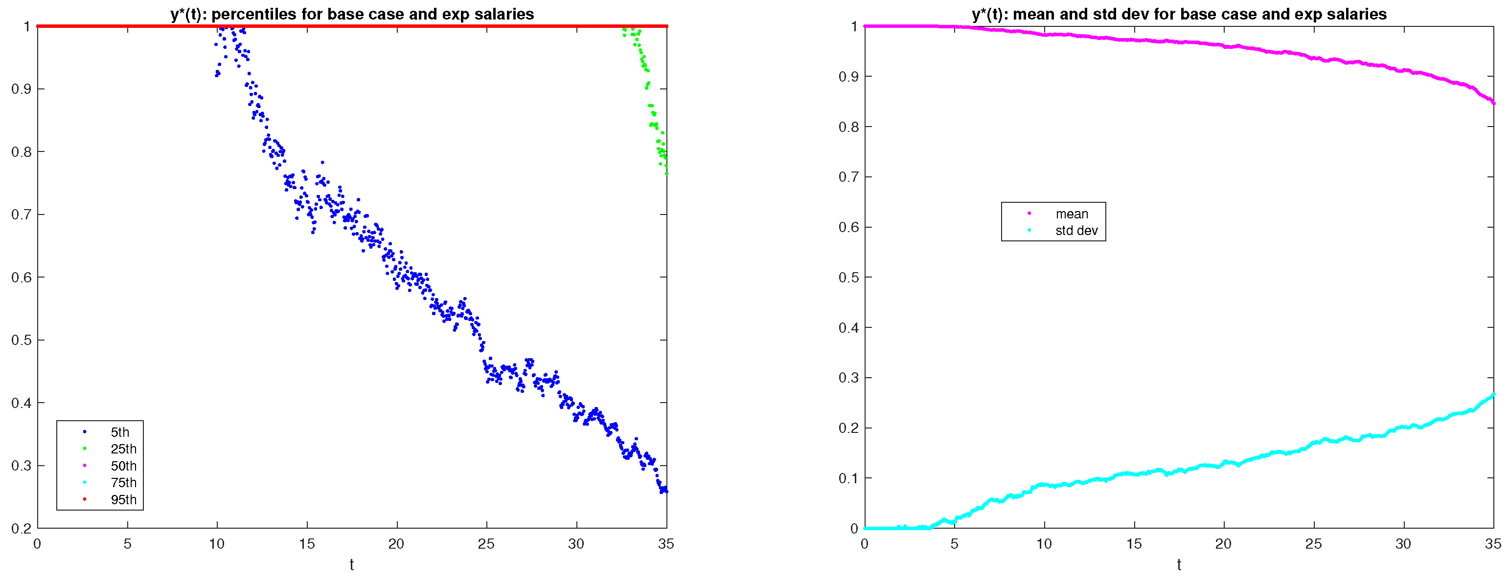
• the two graphs in Figure 1 report percentiles (graph on the left) as well as the mean and standard deviation (graph on the right) of the distribution, over the 1000 scenarios, of the investment strategy $y^{so}\left(t\right)$ for $t\in [0,T]$, for exponential salary growth;
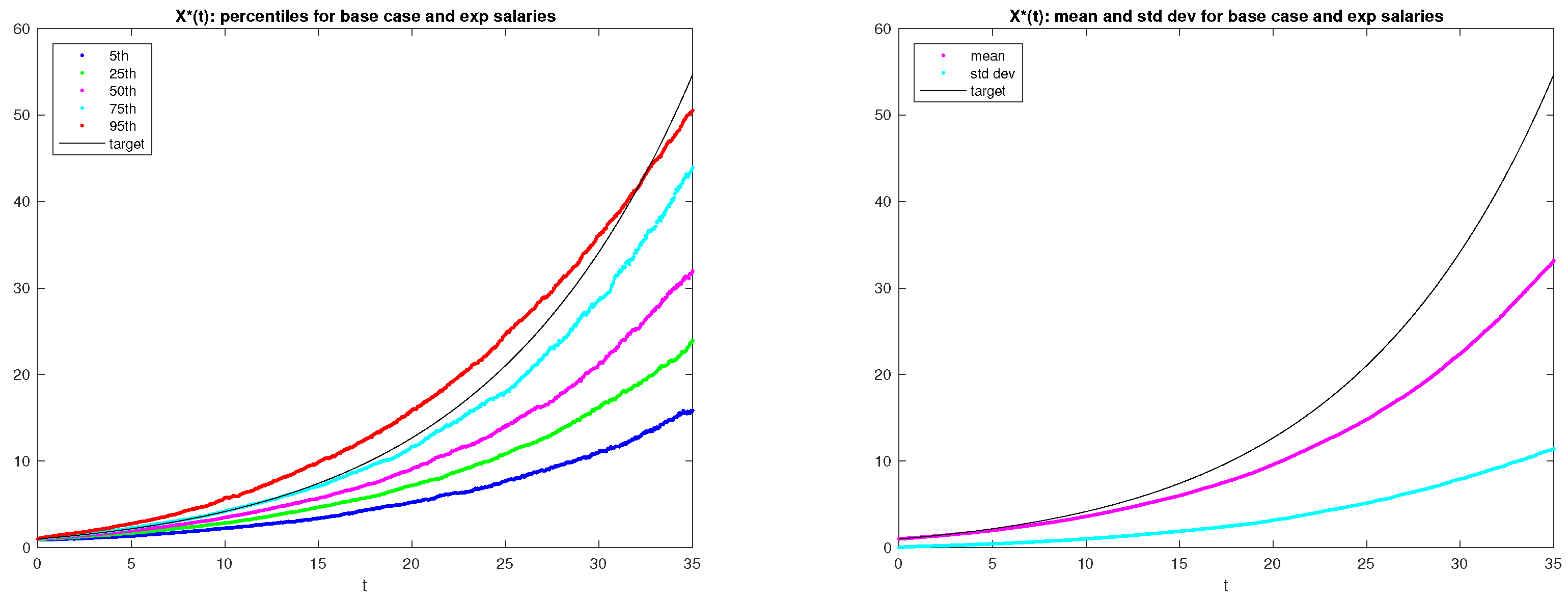
• the two graphs in Figure 2 report percentiles (graph on the left) as well as the mean and standard deviation (graph on the right) of the distribution, over the 1000 scenarios, of the fund $X^{so}\left(t\right)$ for $t\in [0,T]$, for exponential salary growth;
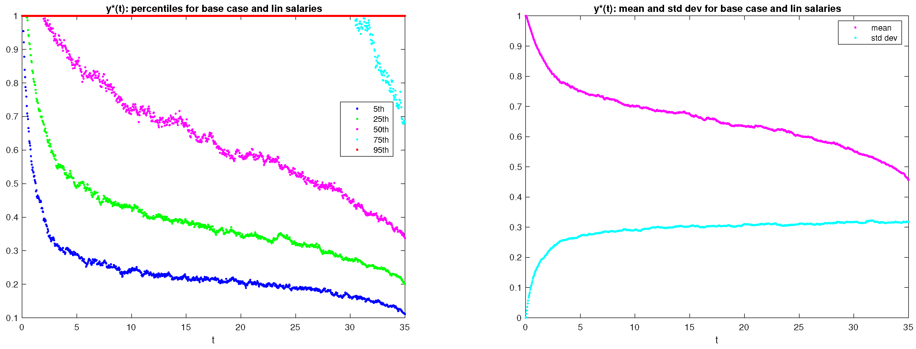
• the two graphs in Figure 3 report percentiles (graph on the left) as well as the mean and standard deviation (graph on the right) of the distribution, over the 1000 scenarios, of the investment strategy $y^{so}\left(t\right)$ for $t\in [0,T]$, for linear salary growth;
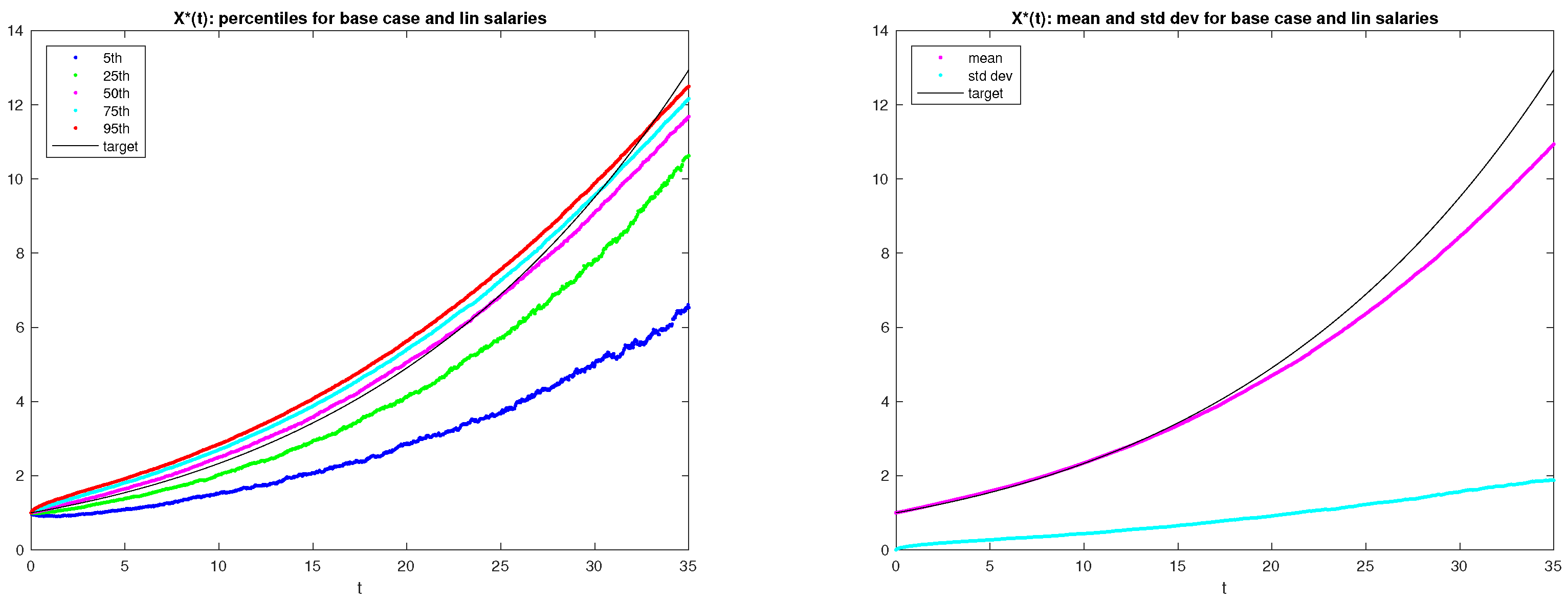
• the two graphs in Figure 4 report percentiles (graph on the left) as well as the mean and standard deviation (graph on the right) of the distribution, over the 1000 scenarios, of the fund $X^{so}\left(t\right)$ for $t\in [0,T]$, for linear salary growth.

We observe the following:

• As expected, with exponential salary growth, the final salary is significantly larger (more than double) than that with linear salary growth; therefore, though the old replacement ratio (that does not depend on the salary growth) is the same ($70\%$), the old pension is much larger with a dynamic career than with a stagnant one.
• The investment strategy for the exponential growth is remarkably riskier than that for the linear growth: for the exponential growth in almost $75\%$ of cases, the portfolio is entirely invested in the risky asset for all t, while for the linear growth all percentiles of $y^{so}\left(t\right)$ (apart from the 95th one) decrease gradually from 1 to 0 over time. The larger riskiness of the strategy for the exponential growth is due to the larger gap between the old and the new pension, see next point.
• With exponential salary growth the gap between the old and the new pension is larger than that with linear salary growth: the old replacement ratio is $70\%$ in both cases, but the new replacement ratio (that does depend on the salary growth) is $32\%$ for the exponential growth and $51\%$ for the linear growth; the larger gap to fill in for the exponential increase entails riskier strategies, and the smaller gap to fill in for the linear increase entails less risky strategies; these results seem to suggest that the new reform affects to a larger extent workers with a dynamic career than workers with a stagnant career.
• With both salary increases, on average the investment in the risky asset decreases over time and approaches 0 when retirement approaches; this result is in line with previous results on optimal investment strategies for DC pension schemes (see, e.g., Haberman and Vigna (2002)) and is consistent with the lifestyle strategy (see Cairns (2000)), which is an investment strategy largely adopted in DC pension funds in the UK.

Finally, because the aim of this work is to reduce the gap between old and new pensions, it is fundamental that the extent to which the gap is reduced be investigated. If the worker joins the pension fund for T years, then at retirement he will receive the new pension $P_n$, the PAYG part of the pension provided by the public pension system, plus the additional pension $P_{add}$, the funded pension provided by the pension fund. Therefore, his total pension will be $P_{tot}$, given by

$$P_{tot}=P_n+P_{add}$$

(55)

where

$$P_{add}=\frac{X^{so}\left(T\right)}{{\ddot{a}}_{65}(1.5\%)}.$$

(56)

In order to compare the old pension with the total pension,

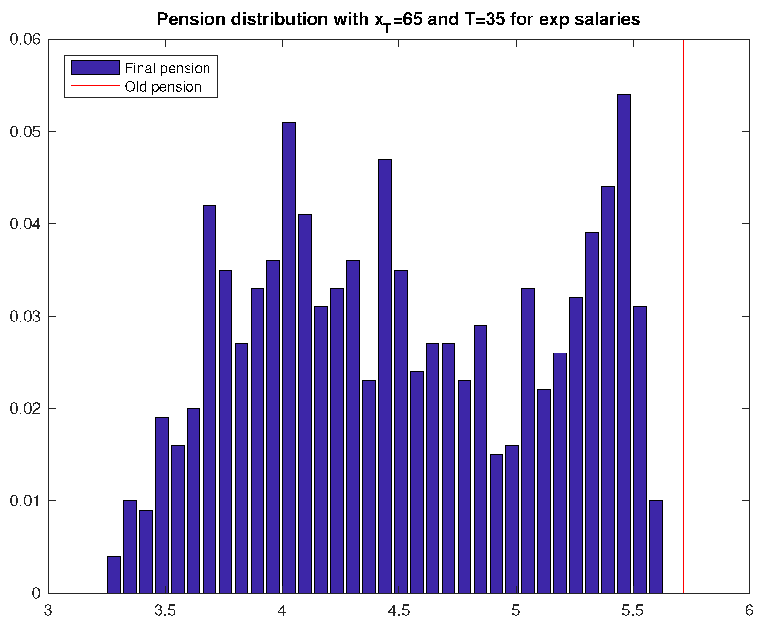
• Figure 5 reports, in the case of exponential salary growth, the distribution, over the 1000 scenarios, of the final pension $P_{tot}$ that the retiree will receive; the old pension $P_o$ is also indicated, as a benchmark.
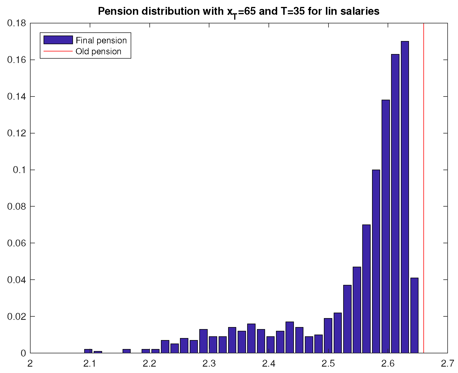
• Figure 6 reports, in the case of linear salary growth, the distribution, over the 1000 scenarios, of the final pension $P_{tot}$ that the retiree will receive; the old pension $P_o$ is also indicated, as a benchmark.

We notice the following:

• In the case of exponential salary growth, the final pension is distributed more uniformly between 3.3 and 5.6 (the old pension being 5.7), while for the linear salary growth, there is a large concentration of final pension on the immediate left of the target, between 2.5 and the target, 2.66.
• That observed above is due to the fact that it is easier to reach the target in the case of a linear increase than in the case of an exponential increase, because (as observed in Point 3 above) the gap between old and new pensions is larger with the exponential increase than with the linear increase.
• The fact that it is relatively easy to approach the target with the linear increase is consistent with the rate of increase of the annual targets $r^{\ast }=4.86\%$ (see Table 1). This rate lies between the return on the riskless asset ($1.5\%$) and the expected return on the risky asset ($6\%$); oppositely, with an exponential salary increase, the rate of increase of annual targets is $r^{\ast }=7.76\%$, which is larger than the expected return on the risky asset.

Remark 4.

We notice that the results of this section are sensitive to the assumptions, particularly to the demographic basis used. We could vary the stochastic date of death by considering different life tables. This would lead to different pension rates in the new system but not in the old one. Therefore, the gap between the old and the new pension would be reduced or enhanced depending on the life table used. In particular, by using an older life table to calculate the annuity price the gap would be reduced, and vice versa. As a consequence, a different gap would affect also the optimal investment strategies.

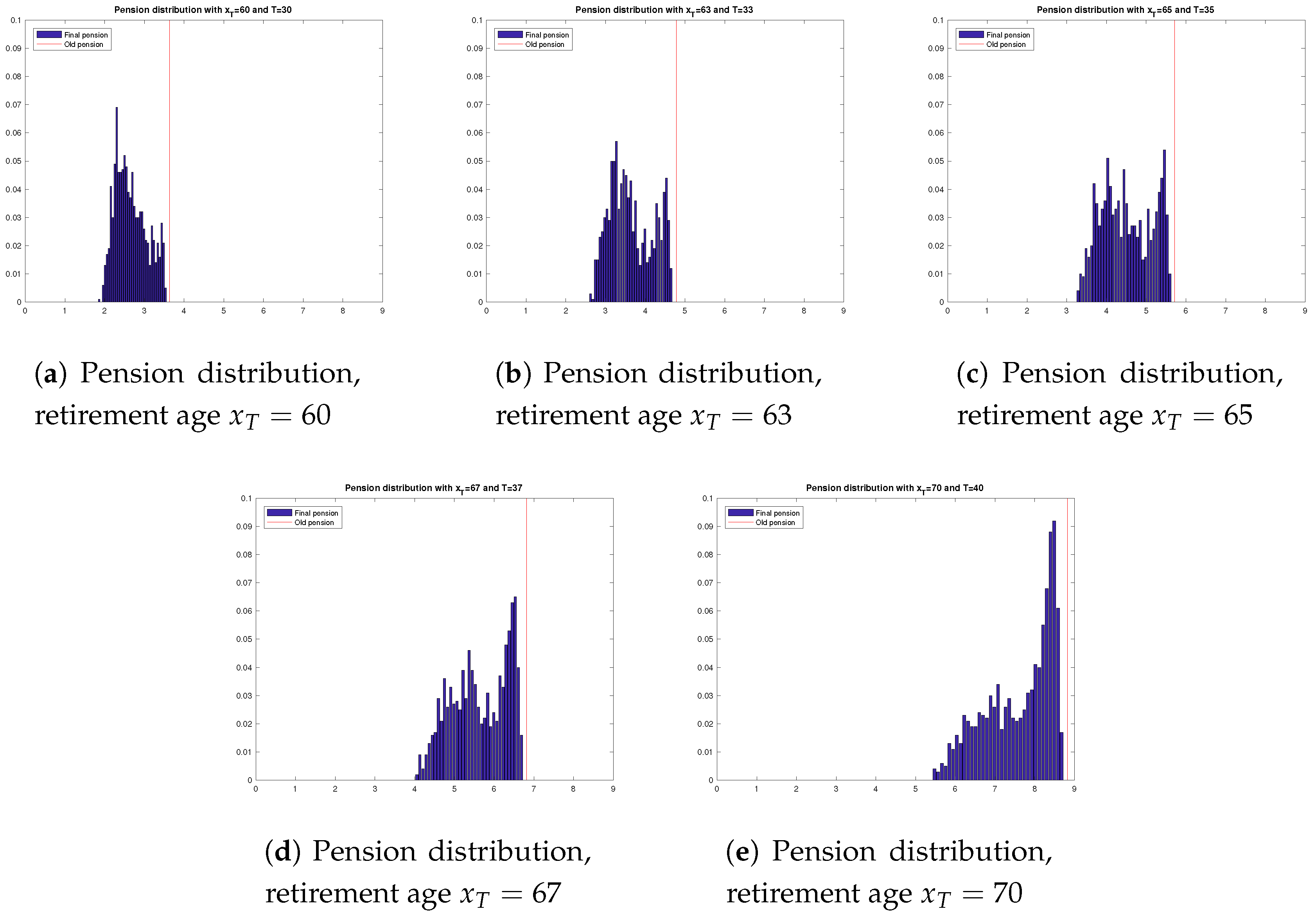
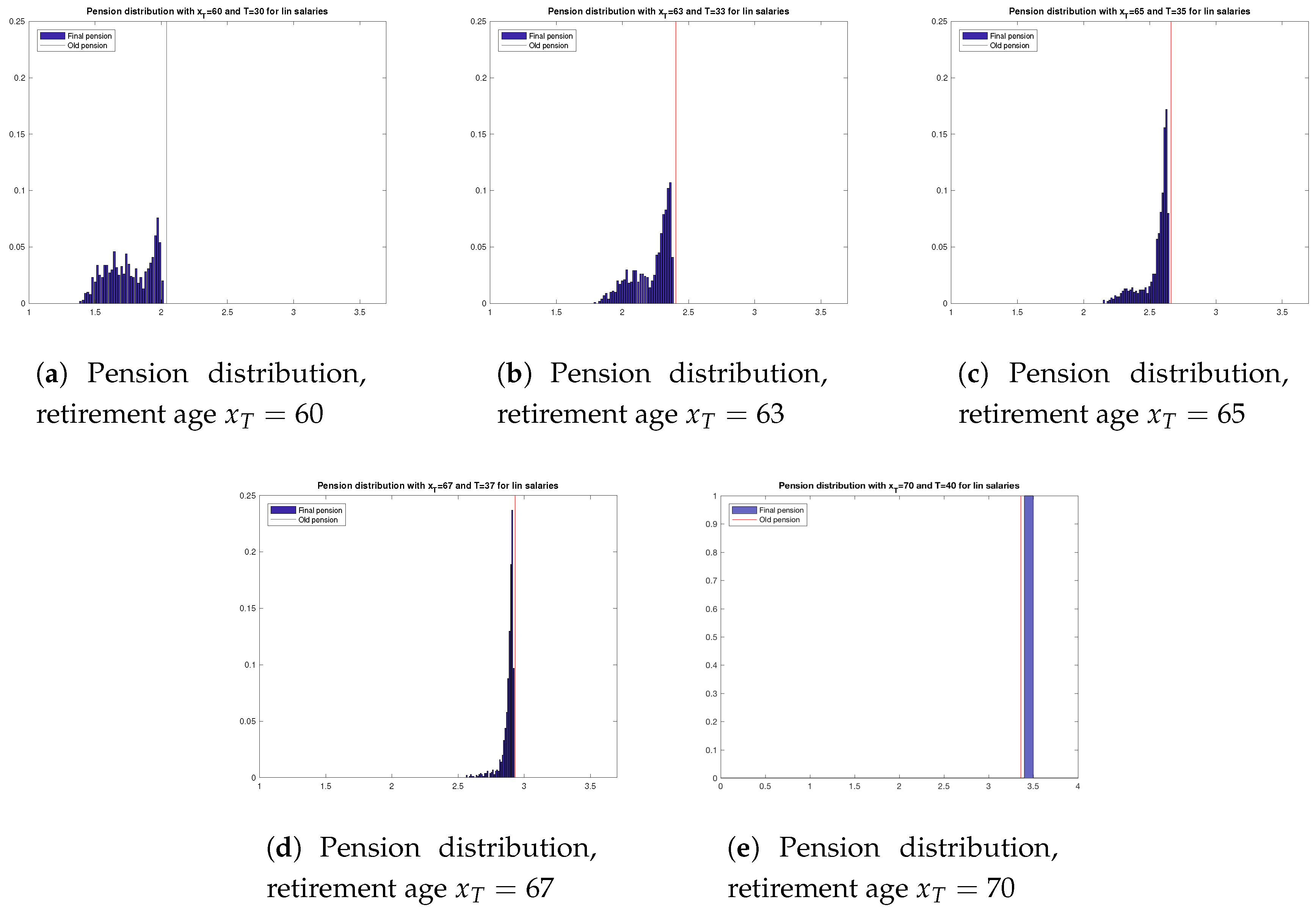
6. Changing the Retirement Age

In Section 5.2, we have set the retirement age equal to 65. It is clear that results strongly depend on retirement age. In this section, we consider different retirement ages, namely, 60, 63, 65, 67, and 70, and investigate how the distribution of the final pension $P_{tot}$ changes accordingly.

Table 2. Annuity value, conversion factor, old and new pension, old and new replacement ratio with exponential and linear salary growth for all retirement ages $X_T$ and working life duration T.

${\mathit{x}}_{\mathit{T}}$	T	${\ddot{\mathit{a}}}_{\mathit{x}}$	${\mathit{\beta }}_{\mathit{x}}$	${\mathit{P}}_{\mathit{o}}^{\mathit{e}}$	${\mathit{P}}_{\mathit{n}}^{\mathit{e}}$	${\mathsf{\Pi }}_{\mathit{o}}^{\mathit{e}}$	${\mathsf{\Pi }}_{\mathit{n}}^{\mathit{e}}$	${\mathit{P}}_{\mathit{o}}^{\mathit{l}}$	${\mathit{P}}_{\mathit{n}}^{\mathit{l}}$	${\mathsf{\Pi }}_{\mathit{o}}^{\mathit{l}}$	${\mathsf{\Pi }}_{\mathit{n}}^{\mathit{l}}$
60	30	20.95	0.048	3.63	1.57	0.6	0.26	2.04	1.26	0.6	0.37
63	33	19.11	0.052	4.78	2.15	0.66	0.3	2.4	1.63	0.66	0.45
65	35	17.88	0.056	5.72	2.66	0.7	0.33	2.66	1.94	0.7	0.51
67	37	16.64	0.06	6.81	3.29	0.74	0.36	2.93	2.3	0.74	0.58
70	40	14.81	0.068	8.82	4.56	0.8	0.41	3.36	2.98	0.8	0.71

reports, for each retirement age considered, $x_T=x$, the annuity value ${\ddot{a}}_x$, the conversion factor from lump sum into pension ${\beta }_x$, and, for both cases of exponential and linear growths, the old pension $P_o$, the new pension $P_n$, the old net replacement ratio ${\mathsf{\Pi }}_o$, and the new net replacement ratio ${\mathsf{\Pi }}_n$.

The graphs in Figure 7 report the pension distribution with the different retirement ages considered in the case of exponential salary growth, while the graphs in Figure 8 report those related to the linear salary increase.

We notice the following:

• The comparison between exponential and linear salary increases confirms what was already observed in Section 5.2 at all ages: the distribution of the final pension is more spread out in the area on the left of the old pension in the case of an exponential salary increase, while it is more peaked immediately on the left of the old pension in the case of the linear target, showing a greater chance of approaching the target in the case of a linear increase.
• With both salary increases, we observe that it is easier to reach the target with an older retirement age: a higher retirement age means a lower gap between the old and the total pension. This is intuitive and expected, and is due to different reasons: (i) because of actuarial fairness principles, as retirement age increases, the price of lifetime annuity decreases; (ii) a higher retirement age also means that the fund grows for a longer period of time, which means that a higher lump sum is converted into pension. These two factors imply that, as retirement age increases, final pension increases, ceteris paribus.
• In the extreme case of linear salary increase and retirement age equal to 70, the difference between the old and the new pension is so small that investing in the riskless asset for the entire working life (40 years) is sufficient to cover the gap, and the final pension $P_{tot}=3.464$ turns out to be higher than the old pension $P_o=3.36$ in $100\%$ of cases.

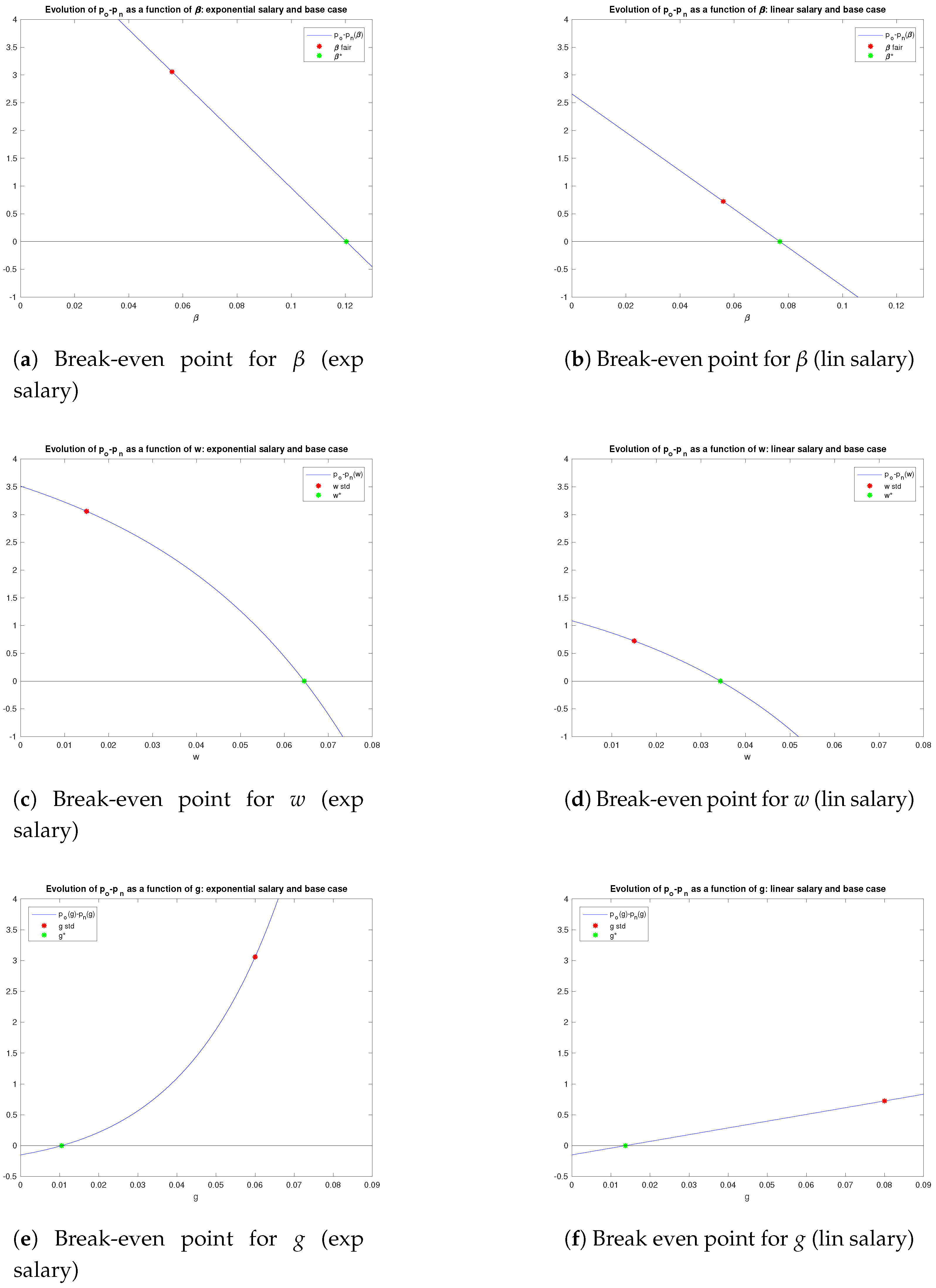
7. Break Even Points

In the previous sections, we have seen that, expectedly, with both salary growths the old pension is larger than the new pension. This result heavily depends on the choice of the parameters and may no longer hold if some parameters change. We have calculated what values of some key parameters would equate the old pension to the new pension, leaving the values of the remaining parameters equal to those of the base case. In particular, we have calculated the break-even points for the parameters w, $\beta$, and g. Figure 9 reports the six plots of the quantity $P_o-P_n$ (difference between the old and the new pension) as a function of $\beta$, g, and w, for exponential and linear salaries. In particular, Figure 9a,c,e report the exponential salary case, while Figure 9b,d,f report the linear salary case. The red point is the base case, and the green point on the $x-$axis is the break-even point that equates the old pension to the new pension.

We notice the following:

• The difference between the old and new pensions decreases with $\beta$, i.e., it increases with the price of the annuity $1/\beta$. This is obvious, because the old pension is not affected by the price of the annuity, while the new pension is affected by $\beta$ and increases with it; therefore, as $\beta$ increases, $P_n$ increases, and $P_o-P_n$ decreases. With exponential increase, the old and new pensions are equal when $\beta =0.12$, which corresponds to the price of the unitary annuity equal to approximately 8.33, against the base value of 17.785; with a linear increase, the old and new pensions are equal when approximately $\beta =0.078$, which corresponds to the price of the unitary annuity equal to 12.82, against the base value of 17.785.
• The difference between the old and new pensions decreases with w. This is again obvious, because the old pension is not affected by the mean GDP growth rate w, while the new pension is affected by w and increases with it; therefore, as w increases, the new pension increases, and the gap between the old and new pensions decreases. With an exponential increase, the old and the new pensions are equal with a mean GDP of approximately $w=6.5\%$. With a linear increase, the old and new pensions are equal with a mean GDP of approximately $w=3.5\%$.
• The difference between the old and new pensions increases with g. This result is interesting, because both the old and new pensions are positively correlated with salary growth g, but to different extents: the old pension is affected by it only via the final salary that is used to calculate the pension income, whereas the new pension is affected by it via the yearly contributions that are paid into the fund and that accumulate until retirement. Figure 9e,f suggest that the impact of g on the old pension is larger than that on the new pension, leading to a larger gap in the case where g increases.
• The break-even point for the salary increase rate is about $g_e=1\%$ for the exponential salary increase, about $g_l=1.5\%$ for a linear increase. This result indicates that, with a sufficiently small salary increase, the old and new pensions coincide. In the presence of salary increase rates that are smaller than the break-even point, the new pension is larger than the old one. This is consistent with what was mentioned in Point 3 in Section 5.2: the effect of the pension reform is more significant for workers with dynamic careers than for workers with stagnant careers.

8. Conclusions

In this paper, we have tackled the issue of the gap between an “old” pre-reform salary-related pension and a “new” post-reform contribution-based pension. We have investigated the extent to which the gap can be reduced by adding to the state pension another pension provided by a DC pension scheme. We have used stochastic optimal control and a target-based approach to find the optimal investment strategy suitable to cover the gap between salary-related and contribution-based pensions. The numerical simulations suggest that the gap between salary-related pensions and contribution-based pensions is larger for workers with dynamic careers than for workers with stagnant careers, which means that it is more difficult for the former to fill the gap than it is for the latter, even when a higher savings capacity is assumed. This is consistent with the results in Bucciol et al. (2017) who find that the presence of the NDC pension system reduces inequality in disposable income. Intuitively, the gap is easier to cover in the case of late retirement, and vice versa. This result is consistent with results in Borella and Coda Moscarola (2010). A slow salary increase associated with a late retirement age can produce a new pension that is almost equal to (or even exceeds) the old pension. Expectedly, the gap reduces when the mean GDP increases and when the price of the annuity decreases. Interestingly, the gap increases when the rate of increase in salary increases.

This paper leaves ample room for further research. For instance, all the parameters of the model could be calibrated to real data, the salaries can be modelled as stochastic processes, sensitivity analysis with respect to the demographic assumption could be performed, and heterogeneity of the agents could be introduced. The search for an optimal retirement age for the new pension system is also in the pipeline for future research.

References

1. Battocchio, Paolo, and Menoncin Francesco. 2004. Optimal pension management in a stochastic framework. Insurance: Mathematics and Economics 34: 79–95. [Google Scholar] [CrossRef]
2. Bordley, Robert, and Marco LiCalzi. 2000. Decision analysis using targets instead of utility functions. Decisions in Economics and Finance 23: 53–74. [Google Scholar] [CrossRef] [Green Version]
3. Borella, Margherita, and Flavia Coda Moscarola. 2006. Distributive properties of pension systems: A simulation of the italian transition from defined benefit to notional defined contribution. Giornale Degli Economisti e Annali di Economia 65: 95–126. [Google Scholar]
4. Borella, Margherita, and Flavia Coda Moscarola. 2010. Microsimulation of pension reforms: Behavioural versus nonbehavioural approach. Journal of Pension Economics and Finance 9: 583–607. [Google Scholar] [CrossRef]
5. Borella, Margherita, and Flavia Coda Moscarola. 2015. The 2011 pension reform in italy and its effects on current and future retirees. 151/15. Turin, TO, Italy: CeRP (Center for Research on Pensions and Welware Policies), pp. 1–54. [Google Scholar]
6. Börsch-Supan, Axel. 2005. From traditional db to notional dc systems: the pension reform process in sweden, italy, and germany. Journal of the European Economic Association 3: 458–465. [Google Scholar]
7. Boulier, Jean-Franç, Shao Juan Huang, and Grégory Taillard. 2001. Optimal management under stochastic interest rates: the case of a protected defined contribution pension fund. Insurance: Mathematics and Economics 28: 173–189. [Google Scholar] [CrossRef]
8. Boulier, Jean-Franç, Stéphane Michel, and Vanessa Wisnia. 1996. Optimizing investment and contribution policies of a defined benefit pension fund. Paper presented at the 6th AFIR Colloquium, Niirnberg, Germany, October 1–3; pp. 593–607. [Google Scholar]
9. Boulier, Jean-Franç, Etienne Trussant, and Daniele Florens. 1995. A dynamic model for pension funds management. Paper presented at the 5th AFIR International Colloquium, Brussels, Belgium; pp. 361–384. Available online: http://www.actuaries.org/AFIR/colloquia/Brussels/Boulier-Florens-Trussant.pdf (accessed on 30 March 2018).
10. Bucciol, Alessandro, Laura Cavalli, Igor Fedotenkov, Paolo Pertile, Veronica Polin, Nicole Sartor, and Alessandro Sommacal. 2017. A large scale olg model for the analysis of the redistributive effects of policy reforms. European Journal of Political Economy 48: 104–127. [Google Scholar] [CrossRef]
11. Cairns, Andrew. 2000. Some notes on the dynamics and optimal control of stochastic pension fund models in continuous time. ASTIN Bulletin 30: 19–55. [Google Scholar] [CrossRef]
12. Cairns, Andrew, David Blake, and Kevin Dowd. 2006. Stochastic lifestyling: Optimal dynamic asset allocation for defined-contribution pension plans. Journal of Economic Dynamic and Control 30: 843–877. [Google Scholar] [CrossRef]
13. Deelstra, Griselda, Martino Grasselli, and Pierre-François Koehl. 2003. Optimal investment strategies in the presence of a minimum guarantee. Insurance: Mathematics and Economics 33: 189–207. [Google Scholar] [CrossRef]
14. Di Giacinto, Marina, Salvatore Federico, and Fausto Gozzi. 2011. Pension funds with a minimum guarantee: A stochastic control approach. Finance and Stochastic 15: 297–342. [Google Scholar] [CrossRef]
15. Di Giacinto, Marina, Salvatore Federico, Fausto Gozzi, and Elena Vigna. 2014. Income drawdown option with minimum guarantee. European Journal of Operational Research 234: 610–24. [Google Scholar] [CrossRef]
16. Gerrard, Russell, Steven Haberman, and Elena Vigna. 2004. Optimal investment choices post retirement in a defined contribution pension scheme. Insurance: Mathematics and Economics 35: 321–42. [Google Scholar] [CrossRef]
17. Gerrard, Russell, Steven Haberman, and Elena Vigna. 2006. The management of de-cumulation risks in a defined contribution pension scheme. North American Actuarial Journal 10: 84–110. [Google Scholar] [CrossRef]
18. Gerrard, Russell, Bjarne Højgaard, and Elena Vigna. 2012. Choosing the optimal annuitization time post retirement. Quantitative Finance 12: 1143–59. [Google Scholar] [CrossRef]
19. Haberman, Steven, and Elena Vigna. 2002. Optimal investment strategies and risk measures in defined contribution pension schemes. Insurance: Mathematics and Economics 31: 35–69. [Google Scholar] [CrossRef]
20. Jessen, Robin, Davud Rostam-Afschar, and Sebastian Schmitz. 2018. How important is precautionary labour supply? Oxford Economic Papers, 1–24. [Google Scholar] [CrossRef]
21. Kahneman, Daniel, and Amos Tversky. 1979. Prospect theory: An analysis of decision under risk. Econometrica 47: 263–91. [Google Scholar] [CrossRef]
22. Li, Duan, and Wan-Lung Ng. 2000. Optimal dynamic portfolio selection: Multiperiod mean-variance formulation. Mathematical Finance 10: 387–406. [Google Scholar] [CrossRef]
23. Menoncin, Francesco, and Elena Vigna. 2017. Mean-variance target-based optimisation for defined contribution pension schemes in a stochastic framework. Insurance: Mathematics and Economics 76: 172–84. [Google Scholar] [CrossRef]
24. Vigna, Elena. 2014. On efficiency of mean-variance based portfolio selection in DC pension schemes. Quantitative Finance 14: 237–58. [Google Scholar] [CrossRef]
25. Zhou, Xun Yu, and Duan Li. 2000. Continuous-time mean-variance portfolio selection: A stochastic LQ framework. Applied Mathematics and Optimization 42: 19–33. [Google Scholar] [CrossRef]
1.
In a NDC pension system pension benefits are paid out from current contributions, as in a PAYG system, but the link between benefits and contributions is defined via a defined-contribution formula. For this reason, a NDC pension system is not funded, it is a PAYG system. For a critical review of the pension reform strategy that turns defined benefit (DB) public PAYG systems into NDC systems see Börsch-Supan (2005).
2.
We will approximate the value r with the Newton–Raphson algorithm.
3.
For a more accurate and realistic model for the salary growth in the Italian context, we refer to the micro-simulation model developed by Borella and Coda Moscarola (2006, 2010).
4.
In the following figures, we have denoted the “sub-optimal” constrained investment strategy by y ( · ) and the “sub-optimal” constrained fund growth by X ( · ) for the sake of simplicity.
Figure 1. Optimal investment strategy; exponential salary growth.
Risks 06 00048 g001
Figure 2. Fund growth; exponential salary growth.
Risks 06 00048 g002
Figure 3. Optimal investment strategy; linear salary growth.
Risks 06 00048 g003
Figure 4. Fund growth; linear salary growth.
Risks 06 00048 g004
Figure 5. Distribution of final pension; exponential salary growth.
Risks 06 00048 g005
Figure 6. Distribution of final pension; linear salary growth.
Risks 06 00048 g006
Figure 7. Pension distribution with different retirement ages and exponential growth.
Risks 06 00048 g007
Figure 8. Pension distribution with different retirement ages and linear growth.
Risks 06 00048 g008
Figure 9. Break-even points w.r.t. β , g and w for exponential and linear salary.
Risks 06 00048 g009