Article

An Optimal Investment Strategy for Insurers in Incomplete Markets

by
Mohamed Badaoui
1,
Begoña Fernández
2 and
Anatoliy Swishchuk
3,*
1
Escuela Superior de Ingeniería Mecánica y Eléctrica, Unidad Zacatenco, IPN. Gustavo A. Madero 07738, Mexico
2
Facultad de Ciencias, Universidad Nacional Autónoma de México (UNAM), Coyoacan 04510, Mexico
3
Department of Mathematics and Statistics, University of Calgary, Calgary, AB T2N 1N4, Canada
*
Author to whom correspondence should be addressed.
Risks 2018, 6(2), 31; https://doi.org/10.3390/risks6020031
Submission received: 23 February 2018 / Revised: 28 March 2018 / Accepted: 29 March 2018 / Published: 3 April 2018
(This article belongs to the Special Issue Recent Development in Actuarial Science and Related Fields)

Abstract

:
In this paper we consider the problem of an insurance company where the wealth of the insurer is described by a Cramér-Lundberg process. The insurer is allowed to invest in a risky asset with stochastic volatility subject to the influence of an economic factor and the remaining surplus in a bank account. The price of the risky asset and the economic factor are modeled by a system of correlated stochastic differential equations. In a finite horizon framework and assuming that the market is incomplete, we study the problem of maximizing the expected utility of terminal wealth. When the insurer’s preferences are exponential, an existence and uniqueness theorem is proven for the non-linear Hamilton-Jacobi-Bellman equation (HJB). The optimal strategy and the value function have been produced in closed form. In addition and in order to show the connection between the insurer’s decision and the correlation coefficient we present two numerical approaches: A Monte-Carlo method based on the stochastic representation of the solution of the insurer problem via Feynman-Kac’s formula, and a mixed Finite Difference Monte-Carlo one. Finally the results are presented in the case of Scott model.

1. Introduction

The problem of investment in a portfolio has attracted the attention of researchers and academics in different settings for decades. Borch (1962) is among the pioneering works that deals with a real life example of the reinsurance market under uncertainty, where participants are insurers that seek to trade risk by acquiring reinsurance contracts. Ferguson (1965) addressed the problem of the expected utility of wealth for the investor in the discrete case. Ferguson conjectured that maximizing exponential utility from terminal wealth is strictly related to minimizing the ruin probability, this conjecture was made under the assumption that the investor is allowed to borrow an unlimited amount of money and without risk-free interest rate. Merton (1969, 1971) in his foundational papers introduced the fundamental classical optimal investment-consumption model in which the interest rate r of the bank account, as well as the mean rate of return μ and volatility σ of the risky asset are constants and the investor seeks to maximize expected utility of terminal wealth. In this case closed form solutions have been obtained. It is worth mentioning that Merton’s work has been a great source of inspiration for many works that have been developed in recent decades. Browne (1995) inspired by Merton (1969, 1971) considered a risk process modeled by a Brownian motion with drift including the possibility of investment in a risky asset, which follows a geometric Brownian motion, but without a risk-free interest rate. Browne verified the conjecture announced by Ferguson and produced a relationship between minimizing the ruin probability and maximizing the exponential utility of terminal wealth, which is a clear connection between insurance and finance. Zariphopoulou (2001) studied the problem of maximizing the expected utility of terminal wealth, when the asset price is described by stochastic volatility models, closed form solutions were provided by proposing a methodology to derive reduced form solutions. Fleming and Hernández-Hernández (2005) considered an extension of the Merton’s problem by allowing a correlation factor between the asset price and an external economic factor. Under a HARA utility function, optimal investment strategy and optimal consumption strategy have been produced as well as the asymptotic limit of investment. Wang (2007), studied the expected utility of insurers by using stochastic control techniques, where explicit optimal strategies are obtained as a solution to a Hamilton-Jacobi-Bellman equation. In Guerra and Centeno (2008), we find the relationship between maximizing the adjustment coefficient and maximizing the expected utility of wealth for the exponential utility function. On the other hand, Yang and Zhang (2005), inspired by Merton as well, considered an optimal investment portfolio modeled by the Cramér-Lundberg process with the possibility of investment in an incomplete market, closed form solution of the optimal strategy maximizing the expected utility of wealth has been produced. In the same context of incomplete market, Henderson (2005) solved the optimal portfolio choice for an investor with exponential utility facing imperfectly hedgeable stochastic income. Badaoui and Fernández (2013) considered an optimization problem, when the insurer preferences are of exponential type for a portfolio that includes a bank account and a risky asset described by stochastic volatility model, which is correlated to an economic factor. A general verification theorem was proved as well as an existence and uniqueness theorem, which led to a closed form of the optimal strategy, when the correlation factor is equal to zero ( ρ = 0 ) . Recently Hata and Yasuda (2017) introduced an extension of (Badaoui and Fernández (2013), Fernández et al. (2008)) by considering a multidimensional linear Gaussian stochastic-factor model. They produce an explicit optimal strategy by solving the matrix Riccati equation.
The main purpose of this paper is to drop the correlation factor condition ( ρ = 0 ), i.e., extending the results obtained in Badaoui and Fernández (2013) to an incomplete market | ρ | < 1 . Following the approach presented in Badaoui and Fernández (2013), an optimal strategy and a value function are obtained in closed form. Since our problem is modeled by a parabolic Partial Differential Equation (PDE) then, by the Feynman-Kac’s formula we obtain a stochastic representation of the solution that allows the use of the Monte-Carlo method, and then the solution of the PDE can be computed only at a small number of points, which is not possible by the Finite Difference method due to stability issues. In order to get some economic explanation on how insurers make their decision in an incomplete market, several numerical simulations are performed by considering the impact of the correlation coefficient on the insurer’s decision. Finally, we propose a mixed Finite Difference Monte-Carlo method, which leads to the same results of simulation obtained by the Monte carlo method. The mixed Finite Difference Monte-Carlo method improves the simulation results obtained in Badaoui and Fernández (2013) and is aimed at avoiding artificial conditions, which may entitle some error in the simulation’s results.
This paper is organized as follows: In Section 2 we define the model of our research and recall some results already proved in Badaoui and Fernández (2013). Section 3 contains the Main Theorem about the existence and uniqueness of the solution of the optimization problem. Section 4 describes the Monte-Carlo method and the mixed Finite Difference Monte-Carlo method. The last section is devoted to presenting some simulation results and providing economic explanation based on the behavior of the value function and the optimal strategy and how the correlation coefficient impacts the insurer’s decision.

2. The Stochastic Volatility Model

This section is devoted to formulating the problem of our research, which consists of a model of an insurance company allowed to invest in a risky asset and a bank account in the presence of stochastic volatility. Let ( Ω , F , P ) be a complete probability space, which carries the following independent stochastic processes:
  • A Poisson process { N t } t 0 with intensity λ > 0 and jump times { T i } i 1 ;
  • A sequence { Y i } i 1 of i.i.d. positive random variables with common distribution G;
  • The Cramér-Lundberg process X t = x + c t i = 1 N t Y i , where x 0 is the initial reserve of the insurance company and c is the constant premium rate;
  • W 1 t and W 2 t are independent standard Brownian motions;
  • The filtration F t is defined by
    F t = σ W 1 s , W 2 s , Y i 1 i N s , 0 s t , i 1
    with the usual conditions Karatzas and Shreve (1988).
In previous articles (Fernández et al. 2008; Yang and Zhang 2005), the asset price was modeled by a geometric Brownian motion given by
d S t = S t ( μ d t + σ d W t ) .
Empirical observations of financial markets show that some indicators of market volatility behave in a highly erratic manner, which makes it unrealistic to assume μ , σ and r constants over long periods of time. This fact has motivated several authors to study the so-called stochastic volatility models (see among others Fouque et al. (2000); Scott (1997); Zariphopoulou (2001)). If the parameters in (1) are stochastic, then motivated by (see, Castañeda and Hernández-Hernández (2005); Fleming and Hernández-Hernández (2005)), the asset price satisfies the following stochastic differential equation:
d S t = S t ( μ ( Z t ) d t + σ ( Z t ) d W 1 t ) with S 0 = 1 ,
where μ ( · ) and σ ( · ) are the return rate and volatility functions, respectively. Z t is an external factor modeled as a diffusion process solving
d Z t = g ( Z t ) d t + β ( ρ d W 1 t + ε d W 2 t ) with Z 0 = z R ,
where ρ 1 , ε = 1 ρ 2 and β 0 . The parameter ρ is the correlation coefficient between W 1 t and W ˜ = ρ W 1 t + ε W 2 t . For ρ < 1 the market is incomplete in the sense that the external factor Z t cannot be traded. The external factor can be written in integral form as
Z t = z + 0 t g ( Z s ) d s + β 0 t d W ˜ s .
Our model also contains a bank account given by the equation
d S t 0 = S t 0 r ( Z t ) d t ,
where r ( · ) is the interest rate function. The process Z t is an external factor that has an impact on both the dynamics of the risky asset prices and the interest paid by the bank account. In Castañeda and Hernández-Hernández (2005) and Fleming and Hernández-Hernández (2005) considered Z t as one of the macroeconomic variables that can be observed by the investor and for instance, can be modeled by the mean reverting Ornstein-Uhlenbeck (O-U) process:
d Z t = γ ( κ Z t ) d t + β d W ˜ t with Z 0 = z ,
where γ and κ are constants and the risky asset price can be given by the Scott model (Cont and Tankov 2003; Fouque et al. 2000):
d S t = S t ( μ 0 d t + e Z t d W 1 t ) with S 0 = 1 .
Here, we assume that μ 0 is constant.
More details about stochastic volatility models can be found in Fouque et al. (2000).
Definition 1.
We say that K = ( K t ) t 0 is an admissible strategy if it is an F t -progressively measurable process such that:
P [ K t C K , 0 t T ] = 1 ,
where C K is a constant, which may depend on the strategy K. We denote the set of admissible strategies as K .
Then if X t is the insurer’s wealth, and he invests an amount K t K in the risky asset and the remaining reserve X t K t in the bank account, then the wealth process X t K : = X ( t , x , z , K ) evolves as follows:
d X t K = c d t + X t K K t S t 0 d S t 0 + K t S t d S t d i = 1 N t Y i ,
which can be represented in the following integral form
X t K = x + 0 t c + ( μ ( Z s ) r ( Z s ) ) K s + r ( Z s ) X s d s + 0 t K s σ ( Z s ) d W 1 s i = 1 N t Y i ,
If at time s < T the wealth of the company is x and the external factor is z, then the wealth process satisfies:
X t s , x , z , K = x + s t c + ( μ ( Z v ) r ( Z v ) ) K v + r ( Z v ) X v d v + s t σ ( Z v ) K v d W 1 v i = N s + 1 N t Y i Z s = z ,
with the convention that i = 1 0 = 0 , and that, when s = 0 we write X t K .
Remark 1.
The case X t K t < 0 means that the insurance company is allowed to borrow from the bank account at the interest rate r ( · ) and reinvest the amount borrowed in the risky asset. In a financial language this means that the insurance is taking a short position in the bank account and a long position in the stock market, which is evident under our approach if we suppose that μ > r and ρ = 0 . The case K t < 0 means that the insurance company is shorting the stock and taking a long position in the bank account which is compatible with our approach if we suppose r > μ and ρ = 0 .
A utility function u : R R is defined as a twice continuously differentiable function, with the property that u ( · ) is strictly increasing and strictly concave. Now we consider the optimization problem that consists in maximizing the expected utility of wealth at time T, i.e., we are interested in the following value function:
V ( s , x , z ) = sup K K E u ( X T s , x , z , K ) .
We say that an admissible strategy K * is optimal if
V ( s , x , z ) = E u ( X T s , x , z , K * ) .
Assumption 1.
The functions μ ( · ) , σ ( · ) and g ( · ) are such that there exists a strong solution for Equations (2) and (4). The general conditions under which the solutions to Equations (2) and (4) exist in the strong sense come from the theory of stochastic differential equations (Øksendal 2003). The function r ( · ) is continuous, positive, and
r ( z ) < μ ( z ) , f o r a l l z R .
The following result establishes a verification theorem, which relates the value function V ( t , x , z ) with the HJB Equation (11).
Theorem 1.
(The Verification Theorem, Badaoui and Fernández (2013)) Assume Assumptions 1 and that there exists a classical solution f ( t , x , z ) C 1 , 2 , 2 ( [ 0 , T ] × R × R ) to the HJB equation:
λ 0 f ( t , x y , z ) f ( t , x , z ) d G ( y ) + sup K R L K f ( t , x , z ) = 0 ,
with terminal condition f ( T , x , z ) = u ( x ) and
L K f ( t , x , z ) = f t + 1 2 σ 2 ( z ) K 2 f x x + 1 2 β 2 f z z + ρ β K σ ( z ) f x z + ( c + ( μ ( z ) r ( z ) ) K + r ( z ) x ) f x + g ( z ) f z ,
such that for each K K
0 T 0 E | f ( s , X s K y , Z s ) f ( s , X s K , Z s ) | 2 d G ( y ) d s < ,
0 T E | K s f x ( s , X s K , Z s ) | 2 d s < ,
0 T E | K s f z ( s , X s K , Z s ) | 2 d s < .
Then for each s [ 0 , t ] , ( x , z ) R 2
f ( s , x , z ) V ( s , x , z ) .
If in addition there exists a bounded measurable function K * ( t , x , z ) such that:
K * ( t , x , z ) a r g m a x K R 1 2 σ 2 ( z ) K 2 f x x + ρ β K σ ( z ) f x z + ( μ ( z ) r ( z ) ) K f x .
Then K t * = K * ( t , X t , Z t ) defines an optimal strategy and
f ( s , x , z ) = V ( s , x , z ) = E [ u ( X T s , x , z , K * ) ] .
Proof. 
For details about the proof we refer to Badaoui and Fernández (2013). ☐
Now we state the Existence and Uniqueness Theorem used later to prove the main Theorem 3 for the incomplete market, which will be given in terms of the following Cauchy problem whose solution has been already proved for the case ρ = 0 in Badaoui and Fernández (2013).
First we need the following Assumptions:
Assumption 2.
We assume that r ( z ) = r constant. Moreover,
g ( z ) ρ β ( μ ( z ) r ) σ ( z )
is bounded and uniformly Lipschitz, and
( μ ( z ) r ) 2 σ 2 ( z )
is bounded with a bounded first derivative.
Theorem 2.
(Existence and Uniqueness Theorem, Badaoui and Fernández (2013)). In addition to Assumptions 1 and 2 we assume:
0 exp 8 α y e r T d G ( y ) <
and
0 y exp α y e r T d G ( y ) < .
Define
θ t = 0 exp α y e r ( T t ) 1 d G ( y ) .
Then for all δ 0 the Cauchy problem
φ t + 1 2 β 2 φ z z + g ( z ) ρ β ( μ ( z ) r ) σ ( z ) φ z 1 δ 1 2 ( μ ( z ) r ) 2 σ 2 ( z ) + c α e r ( T t ) λ θ t φ = 0 φ ( T , z ) = 1
has a unique solution, which satisfies the following conditions:
| φ ( z , t ) | C 1 ( 1 + | z | )
and
| φ z ( z , t ) | C 2 ( 1 + | z | ) ,
where C 1 and C 2 are constants.
Proof. 
For details about the proof we refer to Badaoui and Fernández (2013). ☐
Remark 2.
From the existence and uniqueness Theorem we know that the solution of the PDE (19) admits a stochastic representation given by the Feynman-Kac formula (see, Friedman (1975)):
φ ( z , t ) = E exp 1 δ t T ( μ ( Z ˜ s ) r ) 2 2 σ 2 ( Z ˜ s ) + c α e r ( T s ) λ θ s d s | Z ˜ t = z ,
where Z ˜ u satisfies the following stochastic differential equation:
Z ˜ u = z + t u g ( Z ˜ s ) ρ β ( μ ( Z ˜ s ) r ) σ ( Z ˜ s ) d s + β t u d W ˜ s , t u T
where W ˜ t is a standard Brownian motion and for all ( z , t ) R 2 , φ ( z , t ) > 0 .

3. Existence of a Solution for the Exponential Utility Function

In this section we consider both cases ρ < 1 , which means that the market faced by the insurer is incomplete and | ρ | = 1 for complete market. We will prove the existence and uniqueness of the solution of (11), when the insurer’s preferences are exponential, i.e., the utility function is given by:
u ( x ) = e α x , α > 0 .
The next theorem relates the value function with the HJB given by (11), when the market is incomplete, i.e., | ρ | < 1 .
Theorem 3.
(The Main Theorem) In addition to conditions under which Theorem 2 is satisfied we assume | ρ | < 1 and that there exists C > 0 such that
P μ ( Z t ) r α σ ( Z t ) + ρ β ( 1 ρ 2 ) α φ z ( t , Z t ) φ ( t , Z t ) < C , 0 t T = 1 .
Now let φ be the solution of the Cauchy problem (19). Then the value function defined by (10) has the following form:
V ( t , x , z ) = φ ( t , z ) 1 1 ρ 2 exp α x e r ( T t ) ,
and
K * ( t , z ) = μ ( z ) r α σ 2 ( z ) e r ( T t ) + ρ β ( 1 ρ 2 ) α σ ( z ) φ z ( t , z ) φ ( t , z ) e r ( T t )
is an optimal strategy. When r = ρ = 0 , we have:
V ( t , x , z ) = φ ( z , t ) exp α x ,
and
K * ( t , z ) = μ ( z ) α σ 2 ( z ) .
Proof. 
Following the same approach described in Castañeda and Hernández-Hernández (2005); Zariphopoulou (2001) we assume first that for some δ > 0 the solution of the HJB Equation (11) has the form
f ( t , x , z ) = φ ( z , t ) δ exp { α x e r ( T t ) } ,
where for all ( z , t ) R 2 , the function φ ( z , t ) > 0 , and satisfies the condition (24). In what follows we will use the expressions of the partial derivatives of f (we drop out the dependence on ( t , x , z ) to simplify the notation):
f t = δ φ t φ δ 1 α x r φ δ e r ( T t ) exp α x e r ( T t ) ,
f x = α φ δ e r ( T t ) exp α x e r ( T t ) ,
f x x = α 2 φ δ e 2 r ( T t ) exp α x e r ( T t ) ,
f z = δ φ z φ δ 1 exp α x e r ( T t ) ,
f z z = δ φ z z φ δ 1 + δ ( δ 1 ) φ z 2 φ δ 2 exp α x e r ( T t ) ,
f x z = α δ φ z φ δ 1 e r ( T t ) exp α x e r ( T t ) .
Observe first that from (12) we have
sup K R L K f ( t , x , z ) = sup K R σ 2 ( z ) 2 K 2 f x x + ρ β σ ( z ) K f x z + ( μ ( z ) r ) K f x + f t + 1 2 β 2 f z z + ( c + x r ) f x + g ( z ) f z = S + f t + 1 2 β 2 f z z + ( c + x r ) f x + g ( z ) f z .
Using (29), (30), and (33) we obtain
S = sup K R σ 2 ( z ) 2 K 2 f x x + ρ β σ ( z ) K f x z + ( μ ( z ) r ) K f x = e r ( T t ) exp α x e r ( T t ) φ δ 1 × sup K R σ 2 2 α 2 φ e r ( T t ) K 2 + ρ β α δ σ ( z ) φ z K + ( μ ( z ) r ) α φ K .
Since we have assumed that the function φ is strictly positive, the supremum in the last expression is attained, and the optimal strategy given by
K * ( t , z ) = μ ( z ) r α σ 2 ( z ) e r ( T t ) + δ ρ β α σ ( z ) φ z φ e r ( T t ) ,
is an admissible one from condition (24). Substituting (36) in (35) we obtain
S = exp { α x e r ( T t ) } φ δ 1 ( μ ( z ) r ) 2 2 σ 2 φ + ( μ ( z ) r ) ρ β δ σ φ z + ρ 2 β 2 δ 2 φ z 2 2 φ .
Substituting (37) and the partial derivatives in (34) and (11) we obtain:
0 = δ exp { α x e r ( T t ) } φ δ 1 × φ t + 1 2 β 2 φ z z + g ( z ) ρ β ( μ ( z ) r ) σ ( z ) φ z + 1 2 β 2 ( ρ 2 δ + δ 1 ) φ z 2 φ 1 δ 1 2 ( μ ( z ) r ) 2 σ 2 ( z ) + c α e r ( T t ) λ θ t φ .
Since δ and φ are strictly positive we obtain the following non linear partial differential equation:
0 = φ t + 1 2 β 2 φ z z + g ( z ) ρ β ( μ ( z ) r ) σ ( z ) φ z + 1 2 β 2 ( ρ 2 δ + δ 1 ) φ z 2 φ 1 δ 1 2 ( μ ( z ) r ) 2 σ 2 ( z ) + c α e r ( T t ) λ θ t φ .
We choose δ in such a way that
ρ 2 δ + δ 1 = 0 ,
that is
δ = 1 1 ρ 2 .
Then Equation (39) becomes the Cauchy problem stated in Theorem 2. Finally, from Remark 2 we obtain that the solution is positive, and the proof is completed. ☐
Remark 3.
We observe that the expression given by (26) consists of two terms. The first term represents the Merton strategy Merton (1969) in the absence of the external factor and the second term appears also in Merton (1971) and was interpreted as an intertemporal hedging demand. Henderson (2005) considered an investor facing an imperfectly hedgeable stochastic income and the optimal strategy obtained is similar to the one given by (26) but in a different setting, and finally the optimal strategy depends only on time regardless of the level of wealth.
The assumptions in the theorems are sufficient conditions for the existence and uniqueness of the solution of the PDE involved in this work. Since in general the coefficients of stochastic volatility models are unbounded functions, then usually a truncated strategy is suggested. For any function l C 1 ( R ) , its truncated version will be defined as follows:
l v ( z ) = l ( z ) if a z a , l ( a ) ( 1 + s i n ( z a ) ) if a z a + π 2 , 2 l ( a ) if z a + π 2 , l ( a ) ( 1 s i n ( z + a ) ) if a π 2 z a , 2 l ( a ) if z a π 2 .
We observe that l v is bounded, Lipschitz and that it has a bounded derivative. By this procedure of truncation we get a class of functions that satisfy the sufficient assumptions required to assure the existence and uniqueness of the solution.
Since in the theorems there are various assumptions on functions μ , σ , φ , f . It would be important to give one explicit example of the functions that satisfy all the assumptions of the theorems.
Example 1.
Liang et al. (2011) considered a risky asset with constant volatility and the drift is a linear function of the external factor, it turns out that the model proposed by Liang et al. (2011) is a particular case of our stochastic volatility model. Then, following the same approach by Liang et al. (2011) for which:
μ ( z ) = a z , σ ( z ) = σ a n d g ( z ) = b z ,
where a , σ a n d b are constants, the PDE given by (19) becomes as follows:
φ t + 1 2 β 2 φ z z + b z ρ β ( a z r ) σ φ z 1 δ 1 2 ( a z r ) 2 σ 2 + c α e r ( T t ) λ θ t φ = 0 , φ ( T , z ) = 1 .
Following the same approach by Liang et al. (2011), we seek solutions of the form:
φ ( z , t ) = e J ( t ) z 2 + P ( t ) z + Q ( t ) .
We observe that:
φ t ( z , t ) = ( J ( t ) z 2 + P ( t ) z + Q ( t ) ) φ ( z , t ) ,
φ z ( z , t ) = ( 2 J ( t ) z + P ( t ) ) φ ( z , t ) ,
φ z z ( z , t ) = 2 J ( t ) + ( 2 J ( t ) z + P ( t ) ) 2 φ ( z , t ) .
Substituting the last expression in (40), we get the following nonlinear differential equation:
J ( t ) + 2 β 2 J 2 ( t ) + 2 b a ρ β σ J ( t ) 1 2 a 2 σ 2 δ z 2 + P ( t ) + 2 β 2 J ( t ) a ρ β σ + b P ( t ) + 2 ρ β r σ J ( t ) + a r σ δ z + Q ( t ) + 1 2 β 2 2 J ( t ) + P 2 ( t ) + ρ β r σ P ( t ) 1 δ r 2 2 σ 2 + c α e r ( T t ) λ θ t = 0 ,
and J ( t ) , P ( t ) and Q ( t ) are respectively the solutions of the following ordinary differential equations:
J ( t ) + 2 β 2 J 2 ( t ) + 2 b a ρ β σ J ( t ) 1 2 a 2 σ 2 δ = 0 J ( T ) = 0 ,
P ( t ) + 2 β 2 J ( t ) a ρ β σ + b P ( t ) + 2 ρ β r σ J ( t ) + a r σ δ = 0 P ( T ) = 0 ,
Q ( t ) + 1 2 β 2 2 J ( t ) + P 2 ( t ) + ρ β r σ P ( t ) 1 δ r 2 2 σ 2 + c α e r ( T t ) λ θ t = 0 Q ( T ) = 0 .
Let
τ = 2 β 2 , ϑ = 2 b a ρ β σ , ϵ = 1 2 a 2 σ 2 δ .
By using general methods of ordinary differential equation and assuming that ϑ 2 4 τ ϵ > 0 and since Equation (41) is a Riccati equation; we find the following solutions:
J ( t ) = C ¯ + e t ϑ 2 4 τ ϵ 1 C ¯ e t ϑ 2 4 τ ϵ + τ ϑ 2 4 τ ϵ e t ϑ 2 4 τ ϵ e T ϑ 2 4 τ ϵ ,
where
C ¯ = ϑ ϑ 2 4 τ ϵ 2 τ .
From (44), the solution of (42) is given by:
P ( t ) = e t T 2 β 2 J ( s ) a ρ β σ + b d s t T 2 ρ β r σ J ( s ) + a r σ δ e s T 2 β 2 J ( u ) a ρ β σ + b d u d s .
From (44) and (45) the solution of the equation (43) has the following form:
Q ( t ) = t T 1 2 β 2 2 J ( s ) + P 2 ( s ) + ρ β r σ P ( s ) 1 δ r 2 2 σ 2 + c α e r ( T s ) λ θ s d s .
The optimal strategy (26) becomes explicit as
K * ( t , z ) = a z r α σ 2 e r ( T t ) + ρ β ( 1 ρ 2 ) α σ 2 z J ( t ) + P ( t ) e r ( T t ) ,
where J ( t ) and P ( t ) are given respectively by (44) and (45).
Finally, the solution of the HJB Equation (11) has the following form:
f ( t , x , z ) = e δ J ( t ) z 2 + P ( t ) z + Q ( t ) exp { α x e r ( T t ) } .
When the volatility depends on the external factor as in the case of Scott’s model, where σ ( z ) = e z , it is more difficult to adopt the approach above. Therefore, a numerical approach is implemented to solve the PDE (19).
For a complete market, the correlation between the asset price and the external factor is perfect in the sense that ρ = 1 , then it is obvious that the approach above cannot be adopted to solve the problem of the complete market. In this case we have the following Theorem.
Theorem 4.
Under the same conditions of Theorem 2, assume | ρ | = 1 and let φ ρ be the solution of the following parabolic partial differential equation
φ t ρ + 1 2 β 2 φ z z ρ + g ( z ) ρ β ( μ ( z ) r ) σ ( z ) φ z ρ ( 1 2 ( μ ( z ) r ) 2 σ 2 ( z ) + c α e r ( T t ) λ θ t ) = 0 φ ρ ( T , z ) = 0 .
In addition, assume there exists C > 0 such that
P μ ( Z t ) r α σ ( Z t ) + ρ β α φ z ρ ( t , Z t ) < C , 0 t T = 1 .
Then the value function defined by (10) has the following form:
V ρ ( t , x , z ) = e φ ρ exp α x e r ( T t )
and
K ρ * ( t , z ) = μ ( z ) r α σ 2 ( z ) e r ( T t ) + ρ β α σ ( z ) φ z ρ e r ( T t ) .
Proof. 
In this case we also have that f x x < 0 and the optimal strategy is attained. Substituting the partial derivatives in (11) we obtain directly (without the non linear term) the result. ☐
Remark 4.
The conditions (24) and (47) depend essentially on the external factor Z t , and the coefficients μ and σ. A way to obtain these conditions is to stop the process Z t at a given constant.

Bounds for K ρ * ( 0 , z ) and V ρ ( 0 , x , z )

The purpose of this subsection is to find some bounds for We observe the optimal strategy K ρ * ( 0 , z ) and the utility function V ρ ( t , x , z ) for both cases ρ = 1 and ρ = 1 . Indeed, the solution of the PDE (46) has the following stochastic representation:
φ ρ ( z , t ) = E t T ( μ ( Z ˜ s ρ ) r ) 2 2 σ 2 ( Z ˜ s ρ ) + c α e r ( T s ) λ θ s d s | Z ˜ t ρ = z
where
Z ˜ u ρ = z + t u g ( Z ˜ s ρ ) ρ β ( μ ( Z ˜ s ρ ) r ) σ ( Z ˜ s ρ ) d s + β t u d W ˜ s .
Then
φ ρ ( z , 0 ) = E 0 T ( μ ( Z ˜ s ρ ) r ) 2 2 σ 2 ( Z ˜ s ρ ) + c α e r ( T s ) λ θ s d s | Z ˜ 0 ρ = z 0 T c α e r ( T s ) + λ θ s d s λ T M Y ( α e r T ) 1 ,
where M Y is the moment generating function of Y.
The optimal strategy is given by:
K ρ * ( t , z ) = μ ( z ) r α σ 2 ( z ) e r ( T t ) + ρ β α σ ( z ) φ z ρ e r ( T t ) .
For ρ = 1 , K 1 * ( 0 , z ) is bounded from above as follows:
K 1 * ( 0 , z ) μ ( z ) r α σ 2 ( z ) e r T + λ T ( M Y ( α e r T ) 1 ) β α σ ( z ) e r T .
For ρ = 1 , K 1 * ( 0 , z ) is bounded from below as follows:
K 1 * ( 0 , z ) μ ( z ) r α σ 2 ( z ) e r T λ T ( M Y ( α e r T ) 1 ) β α σ ( z ) e r T .
The value function V ( t , x , z ) is given by:
V ρ ( t , x , z ) = e φ ρ exp α x e r ( T t )
and for | ρ | = 1 we have the following lower bound:
V ρ ( 0 , x , z ) e λ T M Y ( α e r T ) 1 e α x e r T .

4. Numerical Methods

4.1. The Monte Carlo Method

In this subsection we describe the Monte Carlo method for solving the parabolic PDE given by (19). From the existence and uniqueness Theorem we know that the solution of the PDE (19) admits a stochastic representation (see, Friedman (1975)) by:
φ ( z , t ) = E exp 1 δ t T ( μ ( Z ˜ s ) r ) 2 2 σ 2 ( Z ˜ s ) + c α e r ( T s ) λ θ s d s | Z ˜ t = z
where Z ˜ u is given by the following stochastic differential equation:
Z ˜ u = z + t u g ( Z ˜ s ) ρ β ( μ ( Z ˜ s ) r ) σ ( Z ˜ s ) d s + β t u d W ˜ s ,
and W ˜ t , t 0 is a standard Brownian motion. For simplicity we adopt the following notations:
ζ ( t , z ) = 1 δ ( μ ( Z ˜ s ) r ) 2 2 σ 2 ( Z ˜ s ) + c α e r ( T t ) λ θ t ,
h ( z ) : = g ( z ) ρ β ( μ ( z ) r ) σ ( z ) .
To describe the Monte Carlo method for the problem given by Equations (49) and (50) we use the same approach presented in (Asmussen and Glynn 2007; Talay 1996).
Step1: We generate M independent standard Brownian Motion W ˜ t j , for j = 1 M .
Step2: Let D = [ t , T ] , then a uniform grid on D is given by:
t i = t + ( i 1 ) k , i = 1 N , k = ( T t ) / N 1 .
By a Forward Euler scheme (see, Kloeden and Platen (1992)), and for each Brownian motion j = 1 M , Equation (50)
Z ˜ u j = z + t u g ( Z ˜ s ) ρ β ( μ ( Z ˜ s ) r ) σ ( Z ˜ s ) d s + β t u d W ˜ s j ,
is discretized on D as follows:
Z ˜ i j = Z ˜ i 1 j + h ( Z ˜ i 1 j ) k + β ( W ˜ i j W ˜ i 1 j )
where:
t ( i ) : = t i , Z ˜ i j : = Z ˜ t ( i ) j and W ˜ i j : = W ˜ t ( i ) j .
Step3: To estimate the path integral in (49), we use the Trapezoidal rule (see, Calfisch and Moskowitz (1995)). Then the path integral is approximated as follows:
t T ζ ( s , Z ˜ s ) d s = k 2 ζ ( t , z ) + 2 i = 2 N 1 ζ ( t i , Z ˜ i ) + ζ ( T , Z ˜ N ) + o ( k 2 ) .
For j = 1 M , let:
Γ j = t T ζ ( s , Z ˜ s j ) d s = k 2 ζ ( t , z ) + 2 i = 2 N 1 ζ ( t i , Z ˜ i j ) + ζ ( T , Z ˜ N j ) .
Step4: We use the sample path given in (52) to estimate the conditional expectation given by the Feynman-Kac formula (49) as follows:
φ M ( z , t ) : = 1 M i = 1 M e Γ i .
Step5: The strong law of large numbers implies that:
φ M ( z , t ) M φ ( z , t )

4.2. The Mixed Finite Difference-Monte Carlo Method

Since the numerical computations can only be performed on finite domains, the first step is to reduce the Cauchy problem (19) to a bounded domain, i.e., R is replaced by [ a , a ] , and instead of artificial conditions, which were imposed on a and a (see, Badaoui and Fernández (2013)) the boundary conditions will be simulated by the Monte Carlo method as shown by (53). The Cauchy problem to solve is the following:
φ t + 1 2 β 2 φ z z + h ( z ) φ z + ξ ( t , z ) φ = 0 φ ( z , T ) = 1 , z ( a , a ) , φ ( z , t ) = φ M ( t , z ) , ( z , t ) { a , a } × [ 0 , T ] .
For existence and uniqueness results for the Cauchy problem (54) we refer to Friedman (1975).
Now we discretize (54) in the domain D : = [ a , a ] × [ 0 , T ] . A uniform grid on D is given by:
z i = a + ( i 1 ) h , i = 1 N , h = 2 a / N 1 , t j = ( j 1 ) k , j = 1 M , k = T / M 1 .
The space and time derivatives are discretized using finite differences as follows:
φ t ( z i , t j ) φ ( z i , t j ) φ ( z i , t j k ) k , φ z ( z i , t j ) φ ( z i + h , t j ) φ ( z i h , t j ) 2 h , φ z z ( z i , t j ) φ ( z i + h , t j ) 2 φ ( z i , t j ) + φ ( z i h , t j ) h 2 .
Since our Cauchy problem is given with a terminal condition, we follow the same procedure described in Cont and Tankov (2003), but backward in time. We denote by φ i j : = φ ( z i , t j ) the solution on the discretized domain. Then by substituting the derivatives by the expressions given above, (54) becomes:
φ i j φ i j 1 k + 1 2 β 2 φ i + 1 j 2 φ i j + φ i 1 j h 2 + h ( z i ) φ i + 1 j φ i 1 j 2 h + ξ ( t i , z i ) φ i j = 0 ,
and
φ i j 1 k + 1 k β 2 h 2 + ξ ( t i , z i ) φ i j + β 2 2 h 2 + 1 2 h h ( z i ) φ i + 1 j + β 2 2 h 2 1 2 h h ( z i ) φ i 1 j = 0 .
Then for j = 2 M and i = 2 N 1 , φ i j satisfies the following explicit scheme:
φ i j 1 = 1 k β 2 h 2 + k ξ ( t i , z i ) ξ i j + k β 2 2 h 2 + k 2 h h ( z i ) ξ i + 1 j + k β 2 2 h 2 k 2 h h ( z i ) ξ i 1 j .
The final condition is given by:
φ i M = 1 , f o r a l l i = 1 N .
Now the boundary conditions will be given by (53) as follows:
φ 1 j = φ M ( z ( 1 ) , t ( j ) ) f o r a l l j = 1 M 1 , φ N + 1 j = φ M ( z ( N + 1 ) , t ( j ) ) f o r a l l j = 1 M 1 .
Our algorithm given by the explicit scheme, final condition and the boundary conditions is backward in time, forward in space, and hence, by the explicit scheme, the numerical solution can be computed.

4.3. Stability of the Explicit Numerical Scheme

First we assume that the claims are exponentially distributed with parameter ν , then for T < 1 r log ( ν / α ) we get:
θ t = α e r ( T t ) ν α e r ( T t ) .
To ensure that our explicit scheme is numerically stable we need to determine a relationship between the space step and the time step. This relationship ensures that the error does not blow up, when ( z , t ) ( 0 , 0 ) .
Assumption 3.
Under the assumption that | ρ | < 1 , let
M 4 = M 1 + c α λ α e r T ν α e r T ,
M 5 = M 2 + c α e r T λ α ν α ,
and
δ * = 1 ρ 2 .
We define M 1 , M 2 and M 3 as follows:
M 1 = min z [ a , a ] 1 2 ( μ ( z ) r ) 2 σ 2 ( z ) ,
M 2 = max z [ a , a ] 1 2 ( μ ( z ) r ) 2 σ 2 ( z ) ,
M 3 = max z [ a , a ] g ( z ) ρ β ( μ ( z ) r ) σ ( z ) 2 .
Proposition 1.
If
T < 1 r log ν α M 1 + c α λ + M 1 + c α ,
Then a sufficient condition for the stability of the explicit scheme is given as follows:
k 2 < min 2 δ * M 4 h 2 ( δ * M 4 h ) 2 + M 3 2 2 , h 4 ( δ * M 5 ) 2 h 4 + ( M 3 2 + 4 δ * M 5 β 2 ) h 2 + 4 β 4 .
Remark 5.
A simplified representation of the stability condition given in (56) can be written as:
k 2 < C h 4
where
C = max 2 δ * M 4 M 3 2 , 1 4 β 2 .
The approach to get the mathematical conditions under which the explicit scheme is Consistent, Stable and Well-posed is well described in Badaoui and Fernández (2013).

5. Numerical Experiments

5.1. Optimal Investment Strategy and Utility Function

Our purpose in this section is to get some economic interpretation about the impact of the external factor on the insurer decisions. To perform this task we consider the Scott model with some specific parameters described as follows:
The external Factor:
d Z t = γ ( κ Z t ) d t + β d W ˜ t , Z 0 = z
where γ and κ are constants.
The risky asset price is given by:
d S t = S t ( μ 0 d t + e Z t d W 1 t ) with S 0 = 1 ,
and μ 0 is constant.
The values assigned to the parameters involved in this simulation are explicitly given in the following Table 1:
The results of the simulation by using both Monte-Carlo and mixed Finite Difference Monte-Carlo methods are presented in the following figures.
When β = 0.3 the optimal strategy shows a behavior opposite to what was previously obtained:
Remark 6.
The following conclusions are obtained for the particular set of parameters (see, Table 1) used during the simulations.
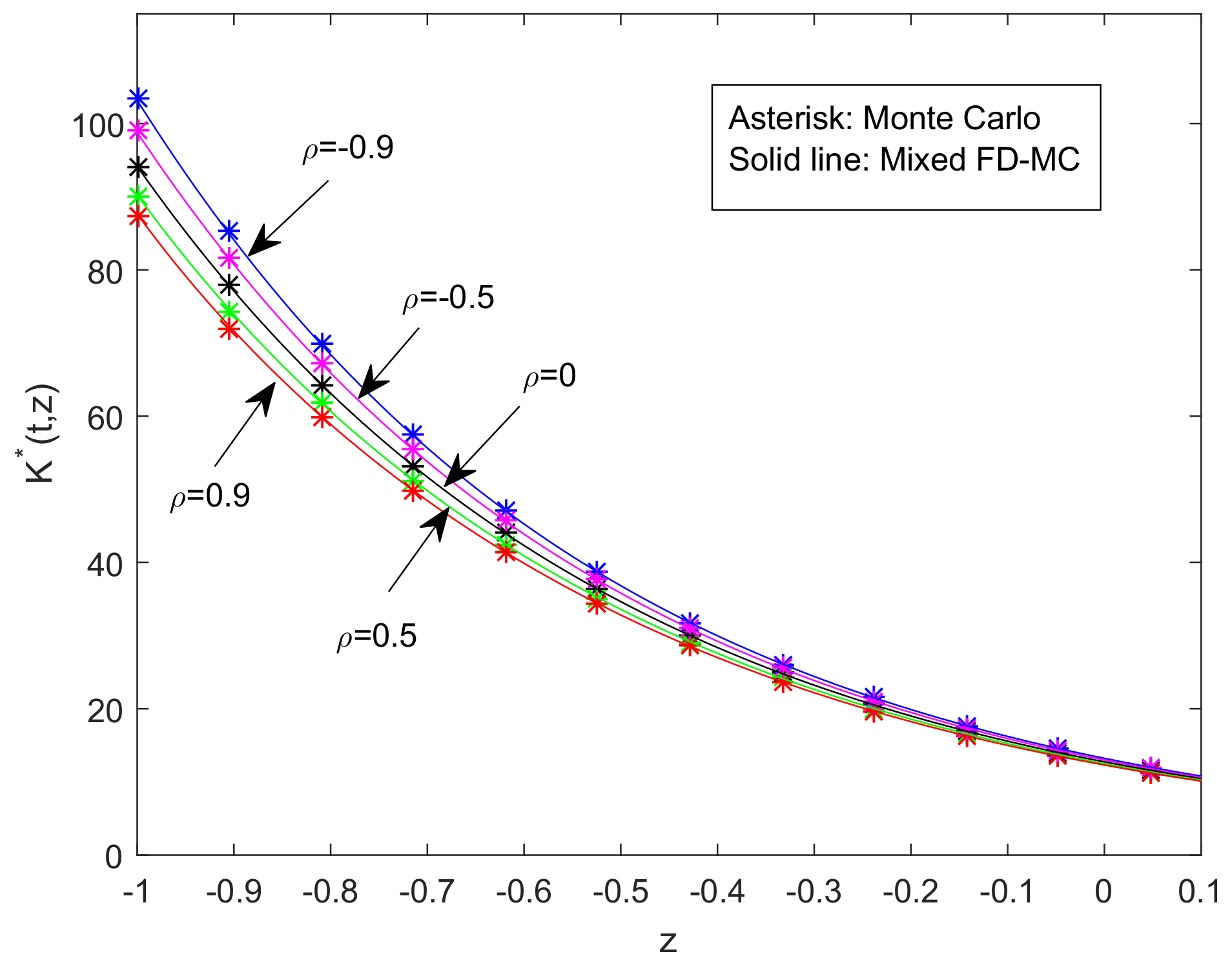
  • From Figure 1, Figure 2, Figure 3 and Figure 4 we observe that the optimal strategy is decreasing with increasing external factor, and as a consequence the insurers invest less in the risky asset regardless the sign of the correlation coefficient.
  • The optimal strategy as a function of the correlation coefficient ρ increases for β > 0 and decreases for β < 0 . When the correlation factor is nonnegative, then the external factor and the risky asset are positively correlated i.e, both are moving in the same direction, which is favorable in a financial environment Schlesinger and Doherty (1985), because the insurer is facing only one source of risk (an increase in the external factor implies an increase in the price of the risky asset) and insurers increase their investment to get more profit. When the correlation coefficient is negative the two risks faced by the insurers are evolving in opposite directions Schlesinger and Doherty (1985), which leads to high risk (an increase in the external factor implies losses in the risky asset), then insurers have to invest less as ρ becomes negatively large, this fact was observed in Zou and Cadenillas (2014) under a deterministic volatility model, when the preferences of the investor are Logarithmic or Exponential.
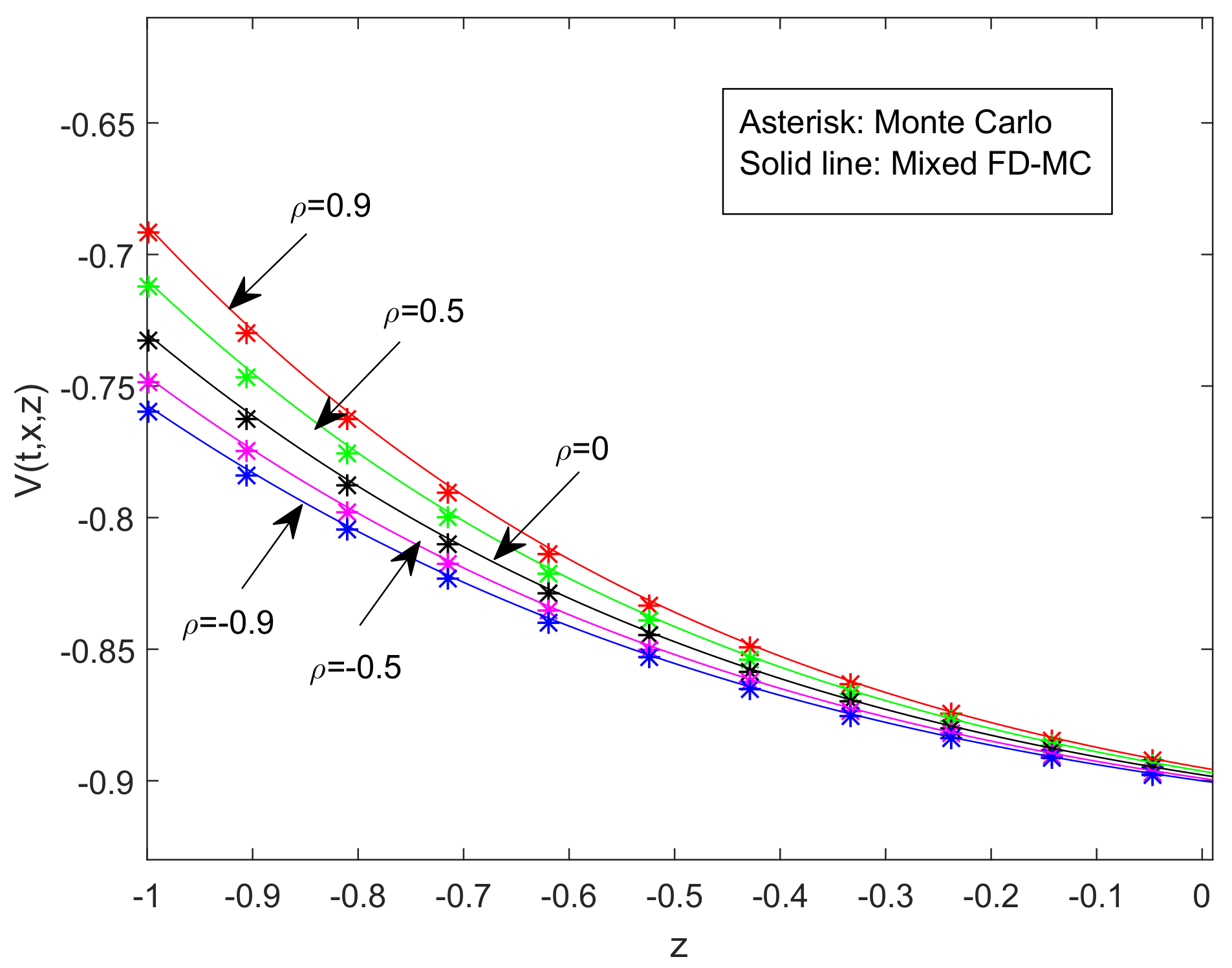
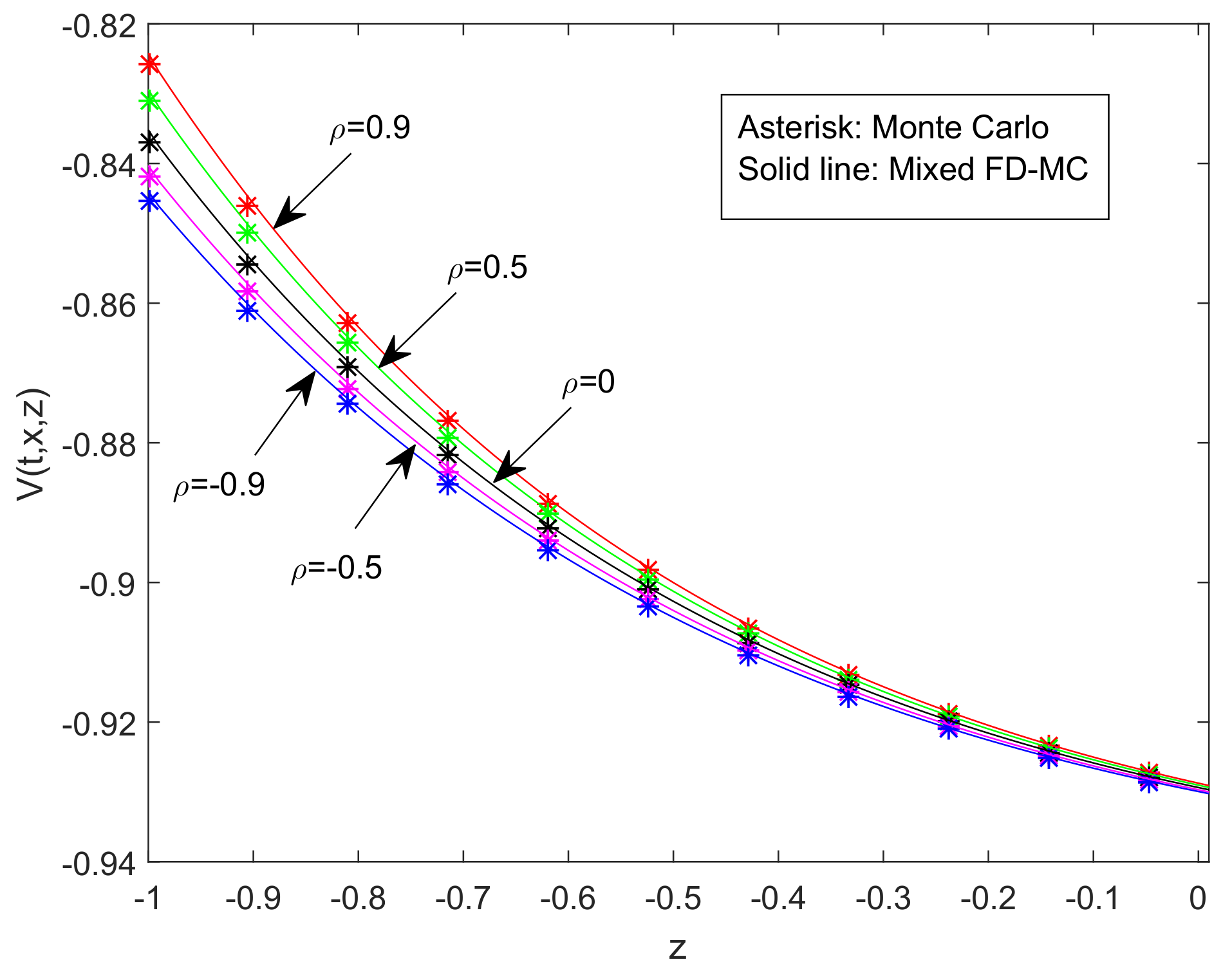
  • The Figure 5 and Figure 6 that show the impact of the external factor on the utility function admit the same economic explanation as those of the optimal strategy.
Remark 7.
Following the same definitions and issues addressed in Schlesinger and Doherty (1985), a real-world example of external factors that determine market incompleteness in the sense considered in this paper and to evaluate whether these factors are negatively or positively correlated with the risky asset, the simplest example is to consider the external factor as any event that can affect the oil price, and a risky asset may be modeled by holding shares in a power generation company (electricity). In this case an increase in the oil price is accompanied by an increase in the price of electricity, then, under the Schlesinger and Doherty (1985) approach, this situation implies a positive correlation coefficient and therefore more benefit for shareholders. However, if instead of the power generation industry, we consider the automobile industry, then the correlation coefficient is negative, which means losses for holders of shares in the automobile industry.
Since analytical results can be derived, the sensitivities to changes in other parameters (initial surplus, premium rate, risk aversion, average claim size, jump intensity of the Poisson process) will be studied in the following way. Let
ω ( z , t ) = E exp 1 δ t T ( μ ( Z ˜ s ) r ) 2 2 σ 2 ( Z ˜ s ) d s | Z ˜ t = z ,
where δ = 1 1 ρ 2 . Then the optimal strategy and the value function given by (26) and (25) can be written as:
K * ( t , z ) = μ ( z ) r α σ 2 ( z ) e r ( T t ) + ρ β ( 1 ρ 2 ) α σ ( z ) ω z ( t , z ) ω ( t , z ) e r ( T t ) ,
V ( t , x , z ) = ω ( t , z ) 1 1 ρ 2 exp t T c α e r ( T s ) λ θ s d s exp α x e r ( T t ) ,
  • Initial Surplus
    • K * ( t , z ) does not depend on x.
    • V ( t , x , z ) x = α e r ( T t ) V ( t , x , z ) > 0 , then V ( t , x , z ) is increasing as a function of x.
  • Premium Rate
    • K * ( t , z ) does not depend on c.
    • V ( t , x , z ) c = t T α e r ( T s ) d s V ( t , x , z ) > 0 , then V ( t , x , z ) increases with the premium rate.
  • Risk Aversion
    • K * ( t , z ) α = 1 α K * ( t , z ) may be negative or positive depending on the parameters of the model.
    • V ( t , x , z ) α = ( t T c e r ( T s ) λ e r ( T s ) E Y exp α Y e r ( T s ) d s + x e r ( T t ) ) V ( t , x , z ) .
      Then the behavior of V (t,x,z) as a function of α depends on the sign of:
      t T c e r ( T s ) λ e r ( T s ) E Y exp α Y e r ( T s ) d s + x e r ( T t )
  • Average Claim size
    • If η = E [ Y ] is the average claim size in the Cramér-Lundberg model, then K * ( t , z ) does not depend on η .
    • V ( t , x , z ) η = λ t T θ s η d s V ( t , x , z ) which depends on the probability distribution of Y. For instance, if the claims are exponentially distributed with parameter ν we know from (55) that:
      θ t = α e r ( T t ) ν α e r ( T t ) = α η e r ( T t ) 1 α η e r ( T t )
      and
      V ( t , x , z ) η = λ α t T e r ( T s ) 1 α η e r ( T s ) d s V ( t , x , z ) < 0 ,
      then V ( t , x , z ) decreases as a function of η .
  • Jump Intensity
    • K * ( t , z ) does not depend on λ .
    • V ( t , x , z ) λ = t T θ s d s V ( t , x , z ) < 0 , then V ( t , x , z ) is deceasing as a function of λ .

5.2. Ruin Probability

Following the approach described in Hata and Yasuda (2017), let X t be the wealth process without investment (The Cramér-Lundberg model) and X t K * the wealth process when the insurer decides to follow the optimal strategy K * . The ruin probability under K * is defined as follows:
Ψ ( x , z ) = P inf 0 t T X t K * 0
and the ruin probability without investment as
Φ ( x ) = P inf 0 t T X t 0 .
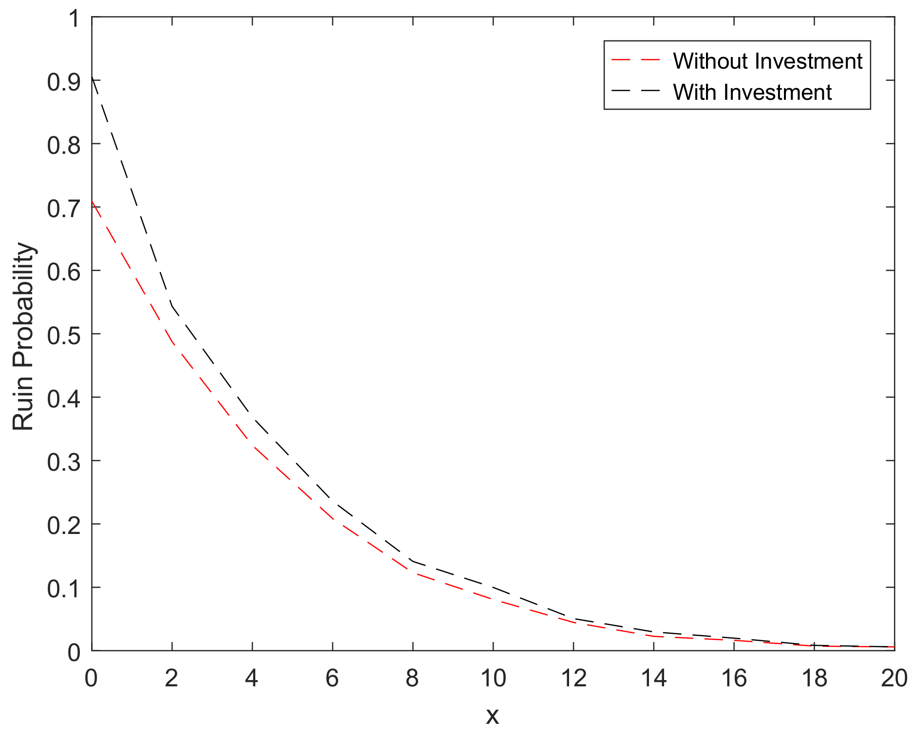
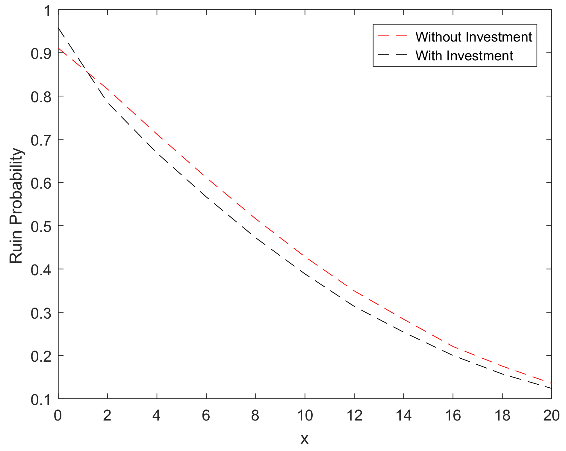
To find the ruin probability we generate N = 5 × 10 4 sample paths for both the wealth process without investment and with investment. The ruin probability is given by the average of the number of paths that fall below zero in each case until maturity time T.
Due to the high computational effort required, we present some simulations under the optimal strategy maximizing the expected utility K * ( t , z ) (which is not necessary the optimal strategy minimizing the ruin probability) for the case ρ = 0 with the following set of parameters given in Table 2:
From the figures of the ruin probability, we observe the following:
Remark 8.
From Figure 7 we observe that the ruin probability decreases for large initial surplus. For a short time horizon, Figure 8 shows that the ruin probability is higher in the presence of investment, but for large time horizon the ruin probability is smaller than in the case without investment.

6. Discussion

  • The approach used in this work is more general because it includes both the study of Complete and Incomplete markets. In the case of ρ 2 1 , the presence of the second Brownian motion cannot be eliminated, which means that the external factor cannot be traded through the risky asset.
  • One consequence of our approach is to recover and improve the behavior of both expected utility and optimal strategy obtained in Badaoui and Fernández (2013), since there is no need to impose artificial boundary conditions, which in this work are approximated via the Monte Carlo method.
  • When the insurer’s preferences are of exponential type, the optimal strategy depends only on time and the external factor regardless of the level of wealth.
  • The Monte Carlo method is a good alternative for the finite difference method, when stochastic representation of the solution is available.

Acknowledgments

The first author would like to thank the support granted by the Project SIP-IPN: 20172231, Conacyt-Mexico and the University of Calgary.

Author Contributions

The authors contributed equally to this work.

Conflicts of Interest

The authors declare no conflict of interest.

References

  1. Asmussen, Søren, and Peter W. Glynn. 2007. Stochastic Simulation, Algorithms and Analysis. New York: Springer. [Google Scholar]
  2. Badaoui, Mohamed, and Begoña Fernández. 2013. An optimal investment strategy with maximal risk aversion and its ruin probability in the presence of stochastic volatility on investments. Insurance: Mathematics and Economics 53: 1–13. [Google Scholar] [CrossRef]
  3. Borch, Karl. 1962. Equilibrium in a reinsuarnce market. Econometrica 30: 424–44. [Google Scholar] [CrossRef]
  4. Browne, Sid. 1995. Optimal investment policies for a firm with a random risk process: Exponential utility and minimizing the ruin probability of ruin. Mathematics of Operations research 20: 937–58. [Google Scholar] [CrossRef]
  5. Calfisch, Russel E., and Bradley Moskowitz. 1995. Modified Monte Carlo methods using quasi-random sequences. In Lecture Notes in Statistics. New York: Springer, vol. 106, pp. 1–16. [Google Scholar]
  6. Castañeda, Netzahualcóyotl, and Daniel Hernández-Hernández. 2005. Optimal consumption-investment problems in incomplete markets with stochastic coefficients. SIAM Journal on Control and Optimization 44: 1322–44. [Google Scholar] [CrossRef]
  7. Cont, Rama, and Peter Tankov. 2003. Financial Modelling with Jump Processes. Orange: Chapman & Hall. [Google Scholar]
  8. Ferguson, Thomas S. 1965. Betting systems which minimize the probability of ruin. Journal of the Society for Industrial and Applied Mathematics 13: 795–818. [Google Scholar] [CrossRef]
  9. Fernández, Begoña, Daniel Hernández-Hernández, Ana Meda, and Patricia Saavedra. 2008. An optimal investment strategy with maximal risk aversion and its ruin probability. Mathematical Methods of Operations Research 68: 159–79. [Google Scholar]
  10. Fleming, Wendell H., and Daniel Hernández-Hernández. 2005. The tradeoff between consumption and investment in incomplete financial markets. Applied Mathematics and Optimization 52: 219–35. [Google Scholar] [CrossRef]
  11. Fouque, Jean-Pierre, George Papanicolaou, and K. Ronnie Sircar. 2000. Derivatives in Financial Markets with Stochastic Volatility. Cambridge: Cambridge Univerrsity Press. [Google Scholar]
  12. Friedman, Avner. 1975. Stochastic Differential Equations and Applications. New York: Academic Press. [Google Scholar]
  13. Guerra, Manuel, and Maria de Lourdes Centeno. 2008. Optimal reinsurance policy: The adjustment coefficient and the expected utility criteria. Insurance: Mathematics and Economics 42: 529–39. [Google Scholar] [CrossRef]
  14. Hata, Hiroaki, and Kazuhiro Yasuda. 2017. Expected exponential utility maximization of insurers with a linear Gaussian stochastic factor model. Scandinavian Actuarial Journal, 1–22. [Google Scholar] [CrossRef]
  15. Henderson, Vicky. 2005. Explicit solutions to an optimal portfolio choice problem with stochastic income. Journal of Economic Dynamics & Control 29: 1237–66. [Google Scholar]
  16. Karatzas, Ioannis, and Steven Shreve. 1988. Brownian Motion and Stochastic Calculus. New York: Springer. [Google Scholar]
  17. Kloeden, Peter E., and Eckhard Platen. 1992. Numerical Solution of Stochastic Differential Equations. Berlin: Springer. [Google Scholar]
  18. Liang, Zhibin, Kam Chuen Yuen, and Junyi Guo. 2011. Optimal proportional reinsurance and investment in a stock market with Ornstein-Uhlenbeck process. Insurance: Mathematics and Economics 49: 207–15. [Google Scholar] [CrossRef]
  19. Merton, Robert C. 1969. Lifetime portfolio selection under uncertainty: The continuous time case. The Review of Economics and Statistics 51: 247–57. [Google Scholar] [CrossRef]
  20. Merton, Robert C. 1971. Optimum consumption and portfolio rules in a continuous time model. Journal of Economic Theory 3: 373–413. [Google Scholar] [CrossRef]
  21. Øksendal, Bernt. 2003. Stochastic Differential Equations: An Introduction with Application. Berlin: Springer. [Google Scholar]
  22. Schlesinger, Harris, and Neil A. Doherty. 1985. Incomplete markets for insurance: An overview. The Journal of Risk and Insurance 52: 402–23. [Google Scholar] [CrossRef]
  23. Scott, Louis O. 1997. Pricing stock options in a jump-diffusion model with stochastic volatility and interest rates: Applications of Fourier inversion methods. Mathematical Finance 7: 413–26. [Google Scholar] [CrossRef]
  24. Talay, Denis. 1996. Probabilistic numerical methods for partial differential equations. Elements of Analysis. In Lecture Notes in Mathematics. Berlin: Springer, pp. 148–196. [Google Scholar]
  25. Wang, Nan. 2007. Optimal investment for an insurer with exponential utility preference. Insurance: Mathematics and Economics 40: 77–84. [Google Scholar] [CrossRef]
  26. Yang, Hailiang, and Lihong Zhang. 2005. Optimal investment for insurer with jump-diffusion risk process. Insurance: Mathematics and Economics 37: 615–34. [Google Scholar] [CrossRef]
  27. Zariphopoulou, Thaleia. 2001. A solution approach to valuation with unhedgeable risks. Finance Stochast 5: 61–82. [Google Scholar] [CrossRef]
  28. Zou, Bin, and Abel Cadenillas. 2014. Optimal investment and risk control policies for an insurer: Expected utility maximization. Insurance: Mathematics and Economics 58: 57–67. [Google Scholar] [CrossRef]
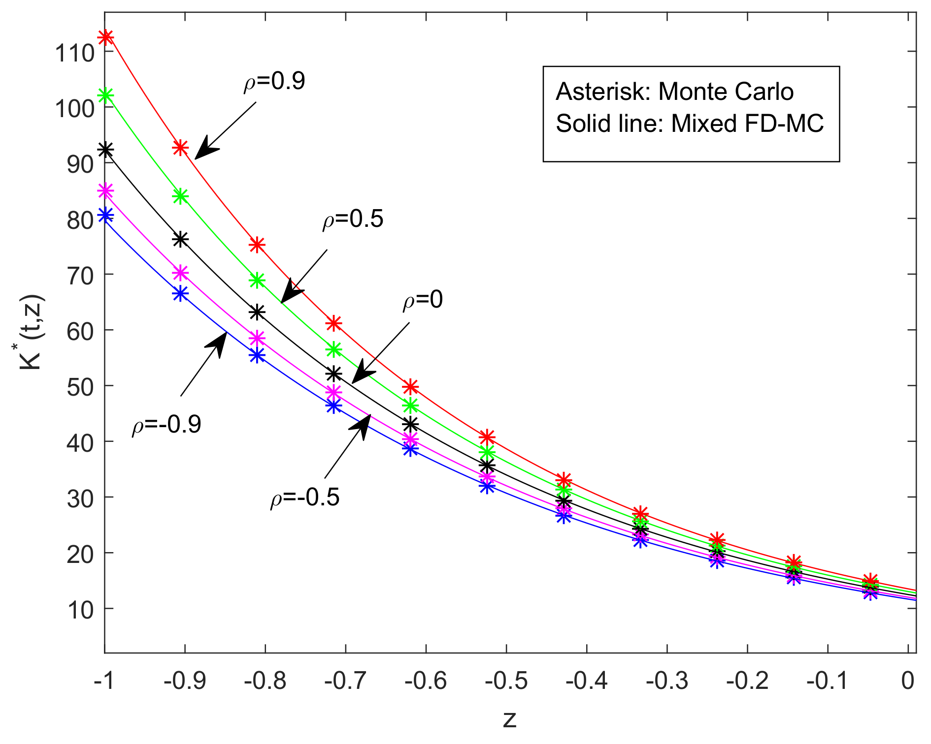
Figure 1. The optimal strategy K * ( t , z ) at t = 0 for different values of ρ .
Risks 06 00031 g001
Figure 2. The optimal strategy K * ( t , z ) at t = 0.5 for different values of ρ .
Risks 06 00031 g002
Figure 3. The optimal strategy K * ( t , z ) at t = 0 for different values of ρ .
Risks 06 00031 g003
Figure 4. The optimal strategy K * ( t , z ) at t = 0.5 for different values of ρ .
Risks 06 00031 g004
Figure 5. The utility function V ( t , x , z ) for t = 0 , x = 0 and different values of ρ .
Risks 06 00031 g005
Figure 6. The utility function V ( t , x , z ) for t = 0.5 , x = 1 and different values of ρ .
Risks 06 00031 g006
Figure 7. The ruin probability when T = 1 and α = 0.1 .
Risks 06 00031 g007
Figure 8. The ruin probability when T = 5 and α = 0.1 .
Risks 06 00031 g008
Table 1. The Parameter values used to simulate K * ( t , z ) and V ( t , x , z ) .
c λ T μ 0 σ r α β γ κ ν a
5310.3 e z 0.040.020.30.1021
Table 2. The Parameter values used to simulate Ψ ( x , z ) and Φ ( x , z ) .
c λ μ 0 σ r β γ κ η z
530.3 e z 00.30.1020