Article

An Individual Claims History Simulation Machine

by
Andrea Gabrielli
* and
Mario V. Wüthrich
RiskLab, Department of Mathematics, ETH Zürich, Rämistrasse 101, 8092 Zürich, Switzerland
*
Author to whom correspondence should be addressed.
Risks 2018, 6(2), 29; https://doi.org/10.3390/risks6020029
Submission received: 5 March 2018 / Revised: 26 March 2018 / Accepted: 27 March 2018 / Published: 30 March 2018

Abstract

:
The aim of this project is to develop a stochastic simulation machine that generates individual claims histories of non-life insurance claims. This simulation machine is based on neural networks to incorporate individual claims feature information. We provide a fully calibrated stochastic scenario generator that is based on real non-life insurance data. This stochastic simulation machine allows everyone to simulate their own synthetic insurance portfolio of individual claims histories and back-test thier preferred claims reserving method.

1. Introduction

The aim of this project is to develop a stochastic simulation machine that generates individual claims histories of non-life insurance claims. These individual claims histories should depend on individual claims feature information such as the line of business concerned, the claims code involved or the age of the injured. This feature information should influence the reporting delay of the individual claim, the claim amount paid, its individual cash flow pattern as well as its settlement delay. The resulting (simulated) individual claims histories should be as ‘realistic’ as possible so that they may reflect a real insurance claims portfolio. These simulated claims then allow us to back-test classical aggregate claims reserving methods—such as the chain-ladder method—as well as to develop new claims reserving methods which are based on individual claims histories. The latter has become increasingly popular in actuarial science, see Antonio and Plat (2014), Hiabu et al. (2016), Jessen et al. (2011), Martínez-Miranda et al. (2015), Pigeon et al. (2013), Taylor et al. (2008), Verrall and Wüthrich (2016) and Wüthrich (2018a) for recent developments. A main shortcoming in this field of research is that there is no publicly available individual claims history data. Therefore, there is no possibility to back-test the proposed individual claims reserving methods. For this reason, we believe that this project is very beneficial to the actuarial community because it provides a common ground and publicly available (synthetic) data for research in the field of individual claims reserving.
This paper is divided into four sections. In this first section we describe the general idea of the simulation machine as well as the chosen data used for model calibration. In Section 2 we describe the design of our individual claims history simulation machine using neural networks. Section 3 focuses on the calibration of these neural networks. In Section 4 we carry out a use test by comparing the real data to the synthetically generated data in a chain-ladder claims reserving analysis. Appendix A presents descriptive statistics of the real data. Since the real insurance portfolio is confidential, we also design an algorithm to generate synthetic insurance portfolios of a similar structure as the real one, see Appendix B. Finally, in Appendix C we provide sensitivity plots of selected neural networks.

1.1. Description of the Simulation Machine

The simulation machine is programmed in the language R. The corresponding .zip-folder can be downloaded from the website:
https://people.math.ethz.ch/~wmario/simulation.html
This .zip-folder contains all parameters, a file readme.pdf which describes the use of our R-functions, as well as the two R-files Functions.V1 and Simulation.Machine.V1. The first R-file Functions.V1 contains the two R-functions Feature.Generation and Simulation.Machine. The former is used to generate synthetic insurance portfolios (this is described in more detail in Appendix B) and the latter to simulate the corresponding individual claims histories (this is described in the main body of this manuscript). The R-file Simulation.Machine.V1 demonstrates the use of these two R-functions, also providing a short chain-ladder claims reserving analysis.

1.2. Procedure of Developing the Simulation Machine

In recent years, neural networks have become increasingly popular in all fields of machine learning. They have proved to be very powerful tools in classification and regression problems. Their drawbacks are that they are rather difficult to calibrate and, once calibrated, they act almost like black boxes between inputs and outputs. Of course, this is a major disadvantage in interpretation and getting deeper insight. However, the missing interpretation is not necessarily a disadvantage in our project because it implies—in back-testing other methods—that the true data generating mechanism cannot easily be guessed.
To construct our individual claims history simulation machine, we design a neural network architecture. This architecture is calibrated to real insurance data consisting of n = 9,977,298 individual claims that have occurred between 1994 and 2005. For each of these individual claims, we have full information of 12 years of claims development as well as the relevant feature information. Together with a portfolio generating algorithm (see Appendix B), one can then use the calibrated simulation machine to simulate as many individual claims development histories as desired.

1.3. The Chosen Data

The chosen data has been preprocessed correcting for wrong entries—for instance, an accident date that is bigger than the reporting date, etc. Moreover, we have dropped claims with missing feature components—for instance, if the age of the injured was missing. However, this was a negligible number of claims that we had to drop, and this does not distort the general calibration. The final (cleaned) data set consists of n = 9,977,298 individual claims histories. The following feature information is available for each individual claim:
  • the claims number ClNr, which serves as a distinct claims identifier;
  • the line of business LoB, which is categorical with labels in { 1 , , 4 } ;
  • the claims code cc, which is categorical with labels in { 1 , , 53 } and denotes the labor sector of the injured;
  • the accident year AY, which is in { 1994 , , 2005 } ;
  • the accident quarter AQ, which is in { 1 , , 4 } ;
  • the age of the injured age (in 5 years age buckets), which is in { 15 , 20 , , 70 } ;
  • the injured part inj_part, which is categorical with labels in { 10 , , 99 } and denotes the part of the body injured;
  • the reporting year RY, which is in { 1994 , , 2016 } .
Not all values in { 10 , , 99 } are needed for the labeling of the categorical classes of the feature component inj_part. In fact, only 46 different values are attained, but for simplicity, we have decided to keep the original labeling received from the insurance company. 46 different labels may still seem to be a lot and a preliminary classification could allow to reduce this number, here we refrain from doing so because each label has sufficient volume.
For all claims i = 1 , , n , we are given the individual claims cash flow ( C i ( j ) ) 0 j 11 , where C i ( j ) is the payment for claim i in calendar year AY i + j —and where AY i denotes the accident year of claim i. Note that we only consider yearly payments, i.e., multiple payments and recovery payments within calendar year AY i + j are aggregated into a single, annual payment C i ( j ) . This single, annual payment can either be positive or negative, depending on having either more claim payments or more recovery payments in that year. The sum over all yearly payments j C i ( j ) of a given claim i has to be non-negative because recoveries cannot exceed payments (this is always the case in the considered data). Remark that our simulation machine will allow for recoveries.
Finally, for claims i = 1 , , n , we are given the claim status process ( I i ( j ) ) 0 j 11 determining whether claim i is open or closed at the end of each accounting year. More precisely, if I i ( j ) = 1 , claim i is open at the end of accounting year AY i + j , and if I i ( j ) = 0 , claim i is closed at the end of that accounting year. Our simulation machine also allows for re-opening of claims, which is quite common in our real data. More description of the data is given in Appendix A.

2. Design of the Simulation Machine Using Neural Networks

In this section we describe the architecture of our individual claims history simulation machine. It consists of eight modeling steps: (1) reporting delay T simulation; (2) payment indicator Z simulation; (3) number of payments K simulation; (4) total claim size Y simulation; (5) number of recovery payments K simulation; (6) recovery size Y simulation; (7) cash flow ( C i ( j ) ) 0 j 11 simulation and (8) claim status ( I i ( j ) ) 0 j 11 simulation. Each of these eight modeling steps is based on one or several feed-forward neural networks. We introduce the precise setup of such a neural network in Section 2.1 for the simulation of the reporting delay T. Before, we present a global overview of the architecture of our simulation machine. Afterwards, in Section 2.1Section 2.8, each single step is described in detail.
To start with, we define the initial feature space X 1 consisting of the original six feature components as
X 1 = { ( LoB , cc , AY , AQ , age , inj_part ) } .
Observe that we drop the claims number ClNr because it does not have explanatory power. Apart from these six feature values, the only other model-dependent input parameters of our simulation machine are the standard deviations for the total individual claim sizes and the total individual recoveries, see Section 2.4 and Section 2.6 below. During the simulation procedure, not all of the subsequent steps (1)–(8) may be necessary—e.g., if we do not have any payments, then there is no need to simulate the claim size or the cash flow pattern. We briefly describe the eight modeling steps (1)–(8).
(1) In the first step, we use the initial feature space X 1 to model the reporting delay T indicating the annualized difference between the reporting year and the accident year.
(2) For the second step, we extend the initial feature space X 1 by including the additional information of the reporting delay T, i.e., we set
X 2 = { ( LoB , cc , AY , AQ , age , inj_part , T ) } .
We use X 2 to model the payment indicator Z determining whether we have a payment or not.
(3) For the third step, we set X 3 = X 2 and model the number of (yearly) payments K.
(4) In the fourth step, we extend the feature space X 3 by including the additional information of the number of payments K, i.e., we set
X 4 = { ( LoB , cc , AY , AQ , age , inj_part , T , K ) } ,
which is used to model the total individual claim size Y.
(5) In the fifth step, we model the number of recovery payments K . We therefore work on the extended feature space
X 5 = LoB , cc , AY , AQ , age , inj_part , T , K , Y .
(6) In the sixth step, we model the total individual recovery Y . To this end, we set X 6 = X 5 . We understand the total individual claim size Y to be net of recovery Y . Thus, the total payment from the insurance company to the insured is Y + Y , paid in K K yearly payments. The total recovery from the insured to the insurance company is Y , paid in K yearly payments.
(7) In the seventh step, the task is to generate the cash flows ( C i ( j ) ) 0 j 11 . Therefore, we have to split the total gross claim amount Y + Y into K K positive payments and the total recovery Y into K negative payments and distribute these K payments among the 12 development years. For this modeling step, we use different feature spaces X 7 a , , X 7 g , all being a subset of
X 7 = LoB , cc , AY , AQ , age , inj_part , T , K , Y , K , Y ,
see Section 2.7 below for more details.
(8) In the last step, we model the claim status process ( I i ( j ) ) 0 j 11 , where we use the feature space
X 8 = LoB , AQ , T , C ( j ) 0 j 11 .
Each of these eight modeling steps (1)–(8) consists of one or even multiple feature-response problems, for which we design neural networks. In the end, the full individual claims history simulation machine consists of 35 neural networks. We are going to describe this neural network architecture in more detail next. We remark that some of these networks are rather similar. Therefore, we present the first neural network in full detail, and for the remaining neural networks we focus on the differences to the previous ones.

2.1. Reporting Delay Modeling

To model the reporting delay, we work with the initial feature space X 1 given in (1). Let n 1 = n = 9,977,298 be the number of individual claims in our data. We consider the (annualized) reporting delays T i , for i = 1 , , n 1 , given by
T i = RY i AY i T = { 0 , , 11 } ,
where AY i is the accident year and RY i the reporting year of claim i. For confidentiality reasons, we have only received data on a yearly time scale (with the additional information of the accident quarter AQ). A more accurate modeling would use a finer time scale.
The three feature components LoB, cc and inj_part are categorical. For neural network modeling, we need to transform these categorical feature components to continuous ones. This could be done by dummy coding, but we prefer the following version because it leads to less parameters. We replace, for instance, the claims code cc by the sample mean of the reporting delay restricted to the corresponding feature label, i.e., for claims code cc = a , we set
a a = a ( a ) = i = 1 n 1 T i 𝟙 { cc i = a } i = 1 n 1 𝟙 { cc i = a } R ,
where cc 1 , , cc n 1 are the observed claims codes. By slight abuse of notation, we obtain a d = 6 dimensional feature space X 1 where we may assume that all feature components of X 1 are continuous. Such feature pre-processing as in (6) will be necessary throughout this section for the components LoB, cc and inj_part: we just replace T i in (6) by the respective response variable. Note that from now on this will be done without any further reference.
The above procedure equips us with the data
D 1 = x 1 , T 1 ) , , ( x n 1 , T n 1 ,
with x 1 , , x n 1 X 1 being the observed features and T 1 , , T n 1 T the observed responses. For an insurance claim with feature x X 1 , the corresponding reporting delay T ( x ) is modeled by a categorical distribution
P T ( x ) = t = π t ( x ) , for t T .
This requires that we model probability functions of the form
π t : X 1 [ 0 , 1 ] , x π t ( x ) ,
satisfying normalization t T π t ( x ) = 1 , for all x X 1 . We design a neural network for the modeling of these probability functions and we estimate the corresponding network parameters from the observations D 1 .
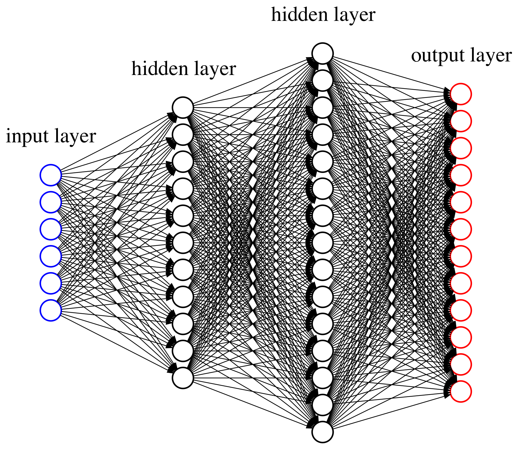
We choose a classical feed-forward neural network with multiple layers. Each layer consists of several neurons, and weights connect all neurons of a given layer to all neurons of the next layer. Moreover, we use a non-linear activation function to pass the signals from one layer to the next. The first layer—consisting of the components x 1 , , x d of a feature x = ( x 1 , , x d ) X 1 —is called input layer (blue circles in Figure 1). In our case, we have d = 6 neurons in this input layer. The last layer is called output layer (red circles in Figure 1) and it contains the categorical probabilities π 0 ( x ) , , π 11 ( x ) . In between these two layers, we choose two hidden layers having q 1 and q 2 hidden neurons, respectively (black circles in Figure 1 with q 1 = 11 and q 2 = 15 ).
More formally, we choose the q 1 hidden neurons z 1 ( 1 ) , , z q 1 ( 1 ) in the first hidden layer as follows
z j ( 1 ) = z j ( 1 ) ( x ) = ϕ w j , 0 ( 1 ) + l = 1 d w j , l ( 1 ) x l , for all j = 1 , , q 1 ,
for given weights ( w j , l ( m ) ) j , l , m and for the hyperbolic tangent activation function
ϕ ( x ) = tanh ( x ) .
This is a centered version of the sigmoid activation function, with range ( 1 , 1 ) . Moreover, we have ϕ = 1 ϕ 2 , which is a useful property in the gradient descent method described in Section 3, below.
The activation is then propagated in an analogous fashion to the q 2 hidden neurons z 1 ( 2 ) , , z q 2 ( 2 ) in the second hidden layer, that is, we set
z j ( 2 ) = z j ( 2 ) ( x ) = ϕ w j , 0 ( 2 ) + l = 1 q 1 w j , l ( 2 ) z l ( 1 ) ( x ) , for all j = 1 , , q 2 .
For the 12 neurons π 0 ( x ) , , π 11 ( x ) in the output layer, we use the multinomial logistic regression assumption
π t ( x ) = exp μ t ( x ) s T exp μ s ( x ) , for all t T ,
with regression functions x μ t ( x ) for all t T given by
μ t ( x ) = β 0 ( t ) + j = 1 q 2 β j ( t ) z j ( 2 ) ( x ) ,
for given weights ( β j ( t ) ) j , t . We define the network parameter α of all involved parameters by
α = w 1 , 0 ( 1 ) , , w q 2 , q 1 ( 2 ) , β 0 ( 0 ) , , β q 2 ( 11 ) R q 1 ( d + 1 ) + q 2 ( q 1 + 1 ) + 12 ( q 2 + 1 ) .
The classification model for the tuples ( x , T ( x ) ) x X 1 is now fully defined and there remains the calibration of the network parameter α and the choice of the hyperparameters q 1 and q 2 . Assume for the moment that q 1 and q 2 are given. In order to fit α to our data D 1 , we aim to minimize a given loss function α L ( α ) . Therefore, we assume that ( x 1 , T 1 ) , , ( x n 1 , T n 1 ) are drawn independently from the joint distribution of ( x , T ( x ) ) . The corresponding deviance statistics loss function of the categorical distribution of our data D 1 is then given by
L ( α ) = L D 1 ( α ) = 2 log i = 1 n 1 t T 𝟙 { T i = t } π t ( x i ) = 2 i = 1 n 1 t T 𝟙 { T i = t } log π t ( x i ) .
The optimal network parameter α is found by minimizing this deviance statistics loss function. We come back to this problem in Section 3.2.1, below. Since for different hyperparameters q 1 and q 2 we get different network structures, every pair ( q 1 , q 2 ) corresponds to a separate model. The choice of appropriate hyperparameters q 1 and q 2 is discussed in Section 3.3, below.
After the calibration of q 1 , q 2 and α to our data D 1 , we can simulate the reporting delay T ( x ) of a claim with given feature x X 1 by using the resulting categorical distribution given by (7). This simulated value will then allow us to go to the next modeling step (2), see (2).
We close this first part with the following remark: Our choice to work with two hidden layers may seem arbitrary since we could also have chosen more hidden layers or just one of them. From a theoretical point of view, one hidden layer would be sufficient to approximate a vast collection of regression functions to any desired degree of accuracy, provided that we have sufficiently many hidden neurons in that layer, see Cybenko (1989) and Hornik et al. (1989). However, these models with large-scale numbers of hidden neurons are known to be difficult to calibrate, and it is often more efficient to use fewer neurons but more hidden layers to get an appropriate complexity in the regression function.

2.2. Payment Indicator Modeling

In our real data, we observe that roughly 29% of all claims can be settled without any payment. For this reason, we model the claim sizes by compound distributions. First, we model a payment indicator Z that determines whether we have a payment or not. Then, conditionally on having a payment, we determine the exact number of payments K. Finally, we model the total individual claim size Y for claims with at least one payment.
In order to model the payment indicator, we work with the d = 7 dimensional feature space X 2 introduced in (2). Let n 2 = n 1 and x 1 , , x n 2 X 2 be the observed features, where this time the reporting delay T is also included. For all i = 1 , , n 2 , we define the number of payments K i and the payments indicator Z i by
K i = j = 0 11 𝟙 C i ( j ) 0 and Z i = 𝟙 { K i > 0 } .
This provides us with the data
D 2 = x 1 , Z 1 ) , , ( x n 2 , Z n 2 .
For a claim with feature x = ( x 1 , , x d ) X 2 , the corresponding payment indicator Z ( x ) is a Bernoulli random variable with
P Z ( x ) = 1 = π ( x ) ,
for a given (but unknown) probability function
π : X 2 [ 0 , 1 ] , x π ( x ) .
Note that this Bernoulli model is a special case of the categorical model of Section 2.1. Therefore, it can be calibrated completely analogously, as described above. However, we emphasize that instead of working with two probability functions π 0 and π 1 for the two categories { 0 , 1 } , we set π ( · ) = π 1 ( · ) , which implies 1 π ( · ) = 1 π 1 ( · ) = π 0 ( · ) . Moreover, the multinomial probabilities (7) simplify to the binomial case
π ( x ) = exp { μ 1 ( x ) } exp { μ 0 ( x ) } + exp { μ 1 ( x ) } = 1 1 + exp { ( μ 1 ( x ) μ 0 ( x ) ) } = 1 1 + exp { μ ( x ) } ,
with regression function
μ : X 2 R , x μ ( x ) = β 0 + j = 1 q 2 β j z j ( 2 ) ( x )
for a neural network with two hidden layers and network parameter α given by
α = w 1 , 0 ( 1 ) , , w q 2 , q 1 ( 2 ) , β 0 , , β q 2 R q 1 ( d + 1 ) + q 2 ( q 1 + 1 ) + ( q 2 + 1 ) .
Finally, the corresponding deviance statistics loss function to be minimized is given by
L ( α ) = L D 2 ( α ) = 2 i = 1 n 2 Z i log π ( x i ) + 1 Z i log ( 1 π ( x i ) ) .
From this calibrated model, we simulate the payment indicator Z ( x ) , which then allows us to go to the next modeling step. If this indicator is equal to one, we move to step (3), see Section 2.3; if this indicator is equal to zero, we directly go to step (8), see Section 2.8.

2.3. Number of Payments Modeling

We use the d = 7 dimensional feature space X 3 = X 2 to model the number of payments, conditioned on the event that the payment indicator Z is equal to one. We define n 3 n 2 to be the number of claims with payment indicator equal to one and order the claims appropriately in i such that Z i = 1 for all i = 1 , , n 3 . Then, we define the number of payments K i as in (9), for all i = 1 , , n 3 . This gives us the data
D 3 = x 1 , K 1 ) , , ( x n 3 , K n 3 .
For a claim with feature x X 3 and payment indicator Z = 1 , we could now proceed as in Section 2.1 in order to model the number of payments K ( x ) . However, the claims with K i = 1 are so dominant in the data that a good calibration of the categorical model (7) becomes difficult. For this reason, we choose a different approach: in a first step, we model the events { K ( x ) = 1 } and { K ( x ) > 1 } , conditioned on { Z = 1 } , and, in a second step, we consider the conditional distribution of K ( x ) , given K ( x ) > 1 . In particular, in the first step we have a Bernoulli classification problem that is modeled completely analogously to Section 2.2, only replacing the data D 2 by
D 3 a = x 1 , 𝟙 { K 1 = 1 } , , x n 3 , 𝟙 K n 3 = 1 .
The case K ( x ) > 1 is then modeled analogously to the categorical case of Section 2.1, with 11 categories and data D 3 b D 3 only considering the claims with more than one payment.
The simulation of the number of payments K ( x ) for a claim with feature x X 3 , reporting delay T and payment indicator Z = 1 needs more care than the corresponding task in Section 2.1: here we have the restriction T + K ( x ) 12 . If T = 11 , then we automatically need to have K ( x ) = 1 . For T < 11 and if the first neural network leads to 𝟙 { K ( x ) = 1 } = 0 , then the categorical conditional distribution for K ( x ) , given K ( x ) > 1 , can only take the values k { 2 , , 12 T } . For this reason, instead of using the original conditional probabilities π 2 ( x ) , , π 12 ( x ) resulting from the second neural network, we use in that case the modified conditional probabilities π k ( x ) , for k { 2 , , 12 T } , given by
π k ( x ) = π k ( x ) l = 2 12 T π l ( x ) .

2.4. Total Individual Claim Size Modeling

For the modeling of the total individual claim size, we add the number of payments K to the previous feature space and work with X 4 given in (3). Let n 4 = n 3 and consider the same ordering of the claims as in Section 2.3. Then, we define the total individual claim size Y i of claim i as
Y i = j = 0 11 C i ( j ) > 0 ,
for all i = 1 , , n 4 . In particular, the total individual claim size Y i is always to be understood net of recoveries. This leads us to the data
D 4 = x 1 , Y 1 ) , , ( x n 4 , Y n 4 .
For a claim with feature x X 4 and payment indicator Z = 1 , we model the total individual claim size Y ( x ) with a log-normal distribution. We therefore choose a regression function
μ : X 4 R
of type (10) for a neural network with two hidden layers. This regression function is used to model the mean parameter of the total individual claim sizes, i.e., we make the model assumption
Y ( x ) Z = 1 LN μ ( x ) , σ + 2 ,
for given variance parameter σ + 2 > 0 . This choice implies
E log Y ( x ) Z = 1 = μ ( x ) and Var log Y ( x ) Z = 1 = σ + 2 .
The density of log Y ( x ) Z = 1 then motivates the choice of the square loss function (deviance statistics loss function)
L ( α ) = L D 4 ( α ) = i = 1 n 4 log Y i μ ( x i ) 2 ,
with network parameter α . The optimal model for the total individual claim size is then found by minimizing the loss function (14), which does not depend on σ + 2 .
This calibrated model together with the input parameter σ + > 0 can be used to simulate the total individual claim size Y ( x ) from (13). Note that the expected claim amount is increasing in σ + 2 , as we have
E Y ( x ) Z = 1 = exp μ ( x ) + σ + 2 2 .

2.5. Number of Recovery Payments Modeling

For the modeling of the number of recovery payments, we use the d = 9 dimensional feature space X 5 introduced in (4). Furthermore, we only consider claims i with K i > 1 , because recoveries may only happen if we have at least one positive payment. We define n 5 n 4 to be the number of claims with more than one payment and order the claims appropriately in i such that K i > 1 for all i = 1 , , n 5 . Then, we define the number of recovery payments K i of claim i as
K i = min j = 0 11 𝟙 C i ( j ) < 0 , 2 ,
for all i = 1 , , n 5 . In particular, for all observed claims i with more than two recovery payments, we set K i = 2 . This reduces combinatorial complexity in simulations (without much loss of accuracy) and provides us with the data
D 5 = x 1 , K 1 ) , , ( x n 5 , K n 5 .
For a claim with feature x X 5 and K > 1 payments, the corresponding number of recovery payments K ( x ) , conditioned on the event { K > 1 } , is a categorical random variable taking values in { 0 , 1 , 2 } , i.e., we are in the same setup as in Section 2.1—with only three categorical classes. Thus, the calibration is done analogously.
This model then allows us to simulate the number of recovery payments K ( x ) . Note that also this simulation step needs additional care: if K = 2 , then we can have at most one recovery payment. Thus, we have to apply a similar modification as given in (12) in this case.

2.6. Total Individual Recovery Size Modeling

The modeling of the total individual recovery size is based on the feature space X 6 = X 5 , given in (4), and we restrict to claims with K i > 0 . The number of these claims is denoted by n 6 n 5 . Appropriate ordering provides us with the total individual recovery Y i of claim i as
Y i = j = 0 11 C i ( j ) 𝟙 C i ( j ) < 0 ,
for all i = 1 , , n 6 . This gives us the data
D 6 = x 1 , Y 1 ) , , ( x n 6 , Y n 6 .
The remaining part is completely analogous to Section 2.4, we only need to replace the standard deviation parameter σ + by a given σ > 0 .

2.7. Cash Flow Pattern Modeling

The modeling of the cash flow pattern is more involved, and we need to distinguish different cases. This distinction is done according to the total number of payments K = 1 , , 12 , the number of positive payments K + = K K = 1 , , 12 as well as the number of recovery payments K = 0 , 1 , 2 .

2.7.1. Cash Flow for Single Payments K = 1

The simplest case is the one of having exactly one payment K = K + = 1 . In this case, we consider the payment delay after the reporting date. We define n 7 a n 3 to be the number of claims with exactly one payment and order the claims appropriately in i such that K i = 1 for all i = 1 , , n 7 a . Then, we define the payment delay S i of claim i as
S i = j = 0 11 j 𝟙 C i ( j ) > 0 T i 0 ,
for all i = 1 , , n 7 a . In other words, we simply subtract the reporting year from the year in which the unique payment occurs. This provides us with the data
D 7 a = x 1 , S 1 ) , , ( x n 7 a , S n 7 a ,
with x 1 , , x n 7 a X 7 a being the observed features, where we use
X 7 a = LoB , cc , AY , AQ , age , inj_part , T , Y
as d = 8 dimensional feature space. For a claim with feature x X 7 a and K = 1 payment, the corresponding payment delay S ( x ) is a categorical random variable assuming values in { 0 , , 11 } . Similarly as for the number of payments, the claims with S i = 0 are rather dominant. Therefore, we apply the same two-step modeling approach as in Section 2.3.
This calibrated model then allows us to simulate the payment delay S ( x ) . For given reporting delay T, we have the restriction T + S ( x ) 11 , which is treated in the same way as in (12). Finally, the cash flow is given by ( C ( j ) ( x ) ) 0 j 11 with
C ( j ) ( x ) = Y , if j = T + S ( x ) , 0 , else .

2.7.2. Cash Flow for Two Payments K = 2

Now we consider claims with exactly two payments. Here we distinguish further between the two cases: (1) both payments are positive, and (2) one payment is positive and the other one negative.
(a) Two Positive Payments
We first consider the case where both payments are positive, i.e., K = K + = 2 and K = 0 . In this case, we have to model the time points of the two payments as well as the split of the total individual claim size to the two payments. For both models, we use the d = 8 dimensional feature space X 7 b = X 7 a , see (16). We define n 7 b n 3 to be the number of claims with exactly two positive payments and no recovery and order them appropriately in i such that K i = 2 and K i = 0 for all i = 1 , , n 7 b . The time points R i ( 1 ) and R i ( 2 ) of the two payments are given by
R i ( 1 ) = min 0 j 11 | C i ( j ) 0 and R i ( 2 ) = max 0 j 11 | C i ( j ) 0 ,
for all i = 1 , , n 7 b . Then, we modify the two-dimensional vector ( R i ( 1 ) , R i ( 2 ) ) to a one-dimensional categorical variable R i by setting
R i = R i ( 2 ) , if R i ( 1 ) = 0 , R i ( 2 ) R i ( 1 ) + k = 12 R i ( 1 ) 11 k , else ,
for all i = 1 , , n 7 b . This leads us to the data
D 7 b = x 1 , R 1 ) , , ( x n 7 b , R n 7 b .
Note that R i is categorical with 12 2 = 66 possible values. That is, we are in the same setup as in Section 2.1—with 66 different classes. Once again, the calibration is done in an analogous fashion as above.
Next, we model the split of the total individual claim size for claims with K = K + = 2 . Let n 7 c = n 7 b , X 7 c = X 7 a , see (16), and define the proportion P i of the total individual claim size Y i that is paid in the first payment by
P i = C i R i ( 1 ) Y i ,
for all i 1 , , n 7 c . This gives us the data
D 7 c = x 1 , P 1 ) , , ( x n 7 c , P n 7 c .
For a claim with feature x X 7 c and K = K + = 2 , the corresponding proportion of its total individual claim size Y that is paid in the first payment is for simplicity modeled by a deterministic function P ( x ) . Note that one could easily randomize P ( x ) using a Dirichlet distribution. However, at this modeling stage, the resulting differences would be of smaller magnitude. Hence, we directly fit the proportion function
P : X 7 c [ 0 , 1 ] , x P ( x ) .
Similarly to the calibration in Section 2.2, we assume a regression function μ : X 7 c R of type (10) for a neural network with two hidden layers. Then, for the output layer, we use
P ( x ) = 1 1 + exp μ ( x )
and as loss function the cross entropy function, see also (11),
L ( α ) = L D 7 c ( α ) = 2 i = 1 n 7 c P i log P ( x i ) + ( 1 P i ) log ( 1 P ( x i ) ) ,
where α is the network parameter containing all the weights of the neural network.
From this model, we can then simulate the cash flow for a claim with K = K + = 2 . First, we simulate R ( x ) . If R ( x ) { 1 , , 11 } , we have R ( 1 ) ( x ) = 0 and R ( 2 ) ( x ) = R ( x ) . If R ( x ) > 11 , we have
R ( 1 ) ( x ) = max 1 k 10 | R ( x ) > u = 12 k 11 u and R ( 2 ) ( x ) = R ( x ) + R ( 1 ) ( x ) k = 12 R ( 1 ) ( x ) 11 k .
The cash flow is given by ( C ( j ) ( x ) ) 0 j 11 with
C ( j ) ( x ) = P ( x ) Y , if j = R ( 1 ) ( x ) , ( 1 P ( x ) ) Y , if j = R ( 2 ) ( x ) , 0 , else .
(b) One Positive Payment, One Recovery Payment
Now we focus on the case where we have K + = 1 positive and K = 1 negative payment. Here we only have to model the time points of the two payments, since we know the total individual claim size as well as the total individual recovery and we assume that the positive payment precedes the recovery payment. The modeling of the time points of the two payments is done as above, except that this time we use the d = 9 dimensional feature space
X 7 d = LoB , cc , AY , AQ , age , inj_part , T , Y , Y ,
where we include the information of the total individual recovery Y . Moreover, we define n 7 d n 3 to be the number of claims with exactly one positive payment and one recovery payment and order the claims appropriately in i such that K i = 2 and K i = 1 for all i = 1 , , n 7 d . This provides us with the data
D 7 d = x 1 , R 1 ) , , ( x n 7 d , R n 7 d ,
with R i defined as in (17). The rest is done as above. We obtain the cash flow ( C ( j ) ( x ) ) 0 j 11 with
C ( j ) ( x ) = Y + Y , if j = R ( 1 ) ( x ) , Y , if j = R ( 2 ) ( x ) , 0 , else .
Remark that we again have combinatorial complexity of 12 2 = 66 for the time points of the two payments. Since data is sparse, for this calibration we restrict to the 35 most frequent distribution patterns. More details on this restriction are provided in the next section.

2.7.3. Cash Flow for More than Two Payments K = 3 , , 12

On the one hand, the models for the cash flows in the case of more than two payments depend on the exact number of payments K. On the other hand, they also depend on the respective numbers of positive payments K + and negative payments K . If we have zero or one recovery payment ( K = 0 , 1 ), then we need to model (a) the time points where the K payments occur and (b) the proportions of the total gross claim amount Y + Y paid in the K + positive payments. If K = 0 , then there are no recovery payments and, thus, Y = 0 . If K = 1 , the recovery payment is always set at the end. In the case of K = 2 recovery payments, in addition to (a) and (b), we use another neural network to model (c) the proportions of the total individual recovery Y paid in the two recovery payments. The time point of the first recovery payment is for simplicity assumed to be uniformly distributed on the set of time points of the 2nd up to the ( K 1 ) -st payment. The second recovery payment is always set at the end. The time point of the first payment is excluded for recovery in our model since we first require a positive payment before a recovery is possible. The three neural networks considered in this modeling part are outlined below in (a)–(c). Afterwards, we can model the cash flow for claims with K = 3 , , 12 payments, see item (d) below.
(a) Distribution of the K Payments
If we have K = 12 payments, then the distribution of these payments to the 12 development years is trivial, as we have a payment in every development year. Since the model is pretty much the same in all other cases K { 3 , , 11 } , we present here the case K = 6 as illustration.
For the modeling of the distribution of the payments to the development years, we slightly simplify our feature space by dropping the categorical feature components cc and inj _ part . Moreover, we simplify the feature LoB with its four categorical classes: since the lines of business one and four as well as the lines of business two and three behave very similarly w.r.t. the cash flow patterns, we merge these lines of business in order to get more volume (and less complexity). We denote this simplified lines of business by LoB . Thus, we work with the d = 8 dimensional feature space
X 7 e = LoB , AY , AQ , age , T , Y , K , Y .
Let n 7 e n 3 be the number of claims with exactly six payments and order the claims appropriately in i such that K i = 6 for all i = 1 , , n 7 e . The time points R i ( 1 ) , , R i ( 6 ) of the six payments are given by
R i ( 1 ) = min 0 j 11 | C i ( j ) 0 and R i ( k ) = min R i ( k 1 ) < j 11 | C i ( j ) 0 ,
for all k = 2 , , 6 and i = 1 , , n 7 e . Then, we use the following binary representation
R i = k = 1 6 2 R i ( k ) + 1 ,
for all i = 1 , , n 7 e , for the time points of the six payments. This leads us to the data
D 7 e = x 1 , R 1 ) , , ( x n 7 e , R n 7 e ,
where x 1 , , x n 7 e X 7 e and R 1 , , R n 7 e A for some set A N . Since there are 12 6 = 924 possibilities to distribute the K = 6 payments to the 12 development years, we have | A | = 924 distribution patterns. To reduce complexity (in view of sparse data), we only allow for the most frequently observed distributions of the payments to the development years. For K = 6 , we work with 21 different patterns, which cover 70 % of all claims with K = 6 . We denote the set containing these 21 patterns by A ˜ . See Table 1 for an overview, for each K = 3 , , 10 , of the number of possible different patterns, the number of allowed different patterns and the percentage of all claims covered with this choice of allowed distribution patterns.
Note that for K = 11 , we allow for all the 12 possible distribution patterns. Going back to the case K = 6 , we denote by n ˜ 7 e n 7 e the number of claims with exactly K = 6 payments and with a distribution of these six payments to the 12 development years contained in the set A ˜ . Then, we modify the data D 7 e accordingly to D ˜ 7 e by only considering the relevant observations in A ˜ . This provides us with a classification problem similar to the one in Section 2.1—with | A ˜ | = 21 classes.
(b) Proportions of the K + = K K Positive Payments
If the number of positive payments K + is equal to one, then the amount paid in this unique positive payment is given by the total gross claim amount Y + Y . That is, we do not need to model the proportions of the positive payments. Since the model is basically the same in all other cases K + { 2 , , 12 } , we present here the case K + = 6 as illustration.
As in the previous part, we use the d = 8 dimensional feature space X 7 f = X 7 e . Let n 7 f n 3 be the number of claims with exactly six positive payments and order the claims appropriately in i such that K i + = K i K i = 6 for all i = 1 , , n 7 f . We define
R i + ( 1 ) = min 0 j 11 | C i ( j ) > 0 and R i + ( k ) = min R i + ( k 1 ) < j 11 | C i ( j ) > 0 ,
for all k = 2 , , 6 and i = 1 , , n 7 f , to be the time points of the six positive payments. Then, we can define
P i ( k ) = C i R i + ( k ) Y i + Y i
to be the proportion of the total gross claim amount Y i + Y i that is paid in the k-th positive, annual payment, for all k = 1 , , 6 and i = 1 , , n 7 f . This equips us with the data
D 7 f = x 1 , P 1 ( 1 ) , , P 1 ( 6 ) , , x n 7 f , P n 7 f ( 1 ) , , P n 7 f ( 6 ) .
For a claim with feature x X 7 f and K + = K K = 6 positive payments, the corresponding proportions P ( 1 ) ( x ) , , P ( 6 ) ( x ) of the total gross claim amount Y + Y that are paid in the six positive payments are for simplicity assumed to be deterministic. Note that we could randomize these proportions by simulating from a Dirichlet distribution, but—as in Section 2.7.2—we refrain from doing so. Hence, we consider the proportion functions
P ( k ) : X 7 f [ 0 , 1 ] , x P ( k ) ( x ) ,
for all k = 1 , , 6 , with normalization k = 1 6 P ( k ) ( x ) = 1 , for all x X 7 f . We use the same model assumptions as in (7) by setting for k = 1 , , 6
P ( k ) ( x ) = exp μ k ( x ) l = 1 6 exp μ l ( x ) ,
for appropriate regression functions μ k : X 7 f R resulting as output layer from a neural network with two hidden layers. As in (19), we consider the cross entropy loss function
L ( α ) = L D 7 f ( α ) = 2 i = 1 n 7 f k = 1 6 P i ( k ) log P ( k ) ( x i ) ,
where α is the corresponding network parameter. This model is calibrated as described in Section 2.1. Remark that if K + = 2 , the model (20) simplifies to the binomial case, see (18).
(c) Proportions of the Recovery Payments if K = 2
In the case of K = 2 recovery payments, we need to model the proportion of the total individual recovery Y that is paid in the first recovery payment. For this, we work with the d = 10 dimensional feature space
X 7 g = LoB , cc , AY , AQ , age , inj_part , T , K , Y , Y .
We denote by n 7 g n 6 the number of claims with exactly two recovery payments and order the claims appropriately in i such that K i = 2 for all i = 1 , , n 7 g . Recall that we set K i = 2 for all claims i with two or more recovery payments, see (15). Moreover, we add all the amounts of the recovery payments done after the second recovery payment to the second one. Let
R i = min 0 j 11 | C i ( j ) < 0
denote the time point of the first recovery payment, for all i { 1 , , n 7 g } . Then, the proportion P i of the total individual recovery Y i that is paid in the first recovery payment is given by
P i = C i ( R i ) Y i ,
for all i = 1 , , n 7 g . This provides us with the data
D 7 g = x 1 , P 1 ) , , ( x n 7 g , P n 7 g .
The remaining modeling part is then done completely analogously to the second part of the two positive payments case (a) in Section 2.7.2.
(d) Cash Flow Modeling
Finally, using the three neural network models outlined above, we can simulate the cash flow for a claim with more than two payments and with feature x X 7 , see (5). We illustrate the case K = 6 . Note that we only allow for cash flow patterns in A ˜ that are compatible with the reporting delay T. We start by describing the case T = 0 . In this case, there is no difficulty and we directly simulate the cash flow pattern R ( x ) A ˜ . This provides us six payments in the time points
R ( 6 ) ( x ) = max 0 j 11 | 2 j + 1 R ( x ) and R ( k ) ( x ) = max 0 j < R ( k + 1 ) ( x ) | 2 j + 1 R ( x ) l = k + 1 6 2 R ( l ) ( x ) + 1 , for k = 1 , , 5 .
For reporting delay T = 1 , the set A ˜ of potential cash flow patterns becomes smaller because some of them have to be dropped to remain compatible with T = 1 . For this reason, we simulate with probability 1 2 a pattern from A ˜ , and with probability 1 2 the six time points R ( 1 ) ( x ) , , R ( 6 ) ( x ) are drawn in a uniform manner from the remaining possible time points in { T = 1 , , 11 } . For T > 1 , the potential subset of patterns in A ˜ becomes (almost) empty. For this reason, we simply simulate uniformly from the compatible configurations in { T , , 11 } .
Having the six time points for the payments, we distinguish the three different cases K { 0 , 1 , 2 } :
Case K = 0 : we calculate the proportions P ( 1 ) ( x ) , , P ( 6 ) ( x ) according to point (b) above and we receive the cash flow ( C ( j ) ( x ) ) 0 j 11 with
C ( j ) ( x ) = P ( l ) ( x ) Y , if j = R ( l ) ( x ) for some 1 l 6 , 0 , else .
Case K = 1 : we have five positive payments with proportions P ( 1 ) ( x ) , , P ( 5 ) ( x ) modeled according to point (b) above. This provides the cash flow ( C ( j ) ( x ) ) 0 j 11 with
C ( j ) ( x ) = P ( l ) ( x ) Y + Y , if j = R ( l ) ( x ) for some 1 l 5 , Y , if j = R ( 6 ) ( x ) , 0 , else .
Case K = 2 : we have four positive payments with proportions P ( 1 ) ( x ) , , P ( 4 ) ( x ) according to point (b) above and two negative payments with proportions P ( x ) and 1 P ( x ) according to point (c) above. The time point of the first recovery R ( x ) is simulated uniformly from the set of time points { R ( 2 ) ( x ) , , R ( 5 ) ( x ) } . Note that the time point R ( 1 ) ( x ) is reserved for the first positive payment and the time point R ( 6 ) ( x ) for the second recovery payment. We write R ˜ ( 1 ) ( x ) , , R ˜ ( 4 ) ( x ) for the time points of the four positive payments. Summarizing, we get the cash flow ( C ( j ) ( x ) ) 0 j 11 with
C ( j ) ( x ) = P ( l ) ( x ) Y + Y , if j = R ˜ ( l ) ( x ) for some 1 l 4 , P ( x ) Y , if j = R ( x ) , ( 1 P ( x ) ) Y , if j = R ( 6 ) ( x ) , 0 , else .
Of course, if K = 3 and K = 2 , we do not need to simulate the proportions of the positive payments, as there is only one positive payment, which occurs in the beginning. Similarly, if K = 12 , we do not need to simulate the time points of the payments, since there is a payment in every development year.
2.8. Claim Status Modeling

Finally, we design the model for the claim status process which indicates whether a claim is open or closed at the end of each accounting year. This process modeling will also allow for re-opening. Similarly to the payments, we do not model the status of a claim or its changes within an accounting year, but only focus on its status at the end of each accounting year. The modeling procedure of the claim status uses two neural networks, which are described below.
We remark that the closing date information was of lower quality in our data set compared to all other information. For instance, some of the dates have been modified retrospectively which, of course, destroys the time series aspect. For this reason, we have decided to model this process in a more crude form, however, still capturing predictive power.

2.8.1. Re-Opening Indicator

We start by modeling the occurrence of a re-opening, i.e., whether a claim gets re-opened after having been closed at an earlier date. We use the d = 15 dimensional feature space
X 8 a = LoB , AQ , T , C ˜ ( j ) 0 j 11 ,
where we do not consider the exact payment amounts, but the simplified version
C ˜ ( j ) = 1 2 , if C ( j ) = 0 , 0 , if C ( j ) 0 and C ( j ) 1 , 000 , 1 2 , if C ( j ) > 1 , 000 ,
for all j = 0 , , 11 . Let n 8 a n denote the number of claims i for which we have the full information ( I i ( j ) ) T i j 11 . For the ease of data processing, we set I i ( j ) = 1 for all development years before claims reporting T i . Then, we can define the re-opening indicator V i as
V i = 1 , if j = 1 11 𝟙 I i ( j ) I i ( j 1 ) = 1 1 , 0 , else ,
for all i = 1 , , n 8 a . In particular, if V i = 1 , then claim i has at least one re-opening, and if V i = 0 , then claim i has not been re-opened. This leads us to the data
D 8 a = { ( x 1 , V 1 ) , , ( x n 8 a , V n 8 a ) } ,
where x 1 , , x n 8 a X 8 a . For a given feature x X 8 a , the corresponding re-opening indicator V ( x ) is a Bernoulli random variable. Thus, model calibration is done analogously to Section 2.2 with, however, a neural network with only one hidden layer.

2.8.2. Closing Delay Indicator for Claims without a Re-Opening

For claims without a re-opening, we model the closing delay indicator determining whether the closing occurs in the same year as the last payment or if the closing occurs later. In case of no payments ( Z i = 0 ), we replace the year of the last payment by the reporting year. We use the same d = 15 dimensional feature space as for the re-opening indicator and set X 8 b = X 8 a , see (21). Let n 8 b n 8 a be the number of claims without a re-opening and order them appropriately in i such that V i = 0 for all i = 1 , , n 8 b . Then, we define the closing delay indicator W i as
W i = 1 , if Z i = 1 and max 0 j 11 | I i ( j ) = 1 max 0 j 11 | C i ( j ) 0 , 1 , if Z i = 0 and max 0 j 11 | I i ( j ) = 1 T i , 0 , else ,
for all i = 1 , , n 8 b . Hence, we have W i = 1 if the closing occurs in a later year compared to the year of the last payment (or in a later year compared to the claims reporting year in case there is no payment) and W i = 0 otherwise. This leads us to the data
D 8 b = { ( x 1 , W 1 ) , , ( x n 8 b , W n 8 b ) } .
For a claim with feature x X 8 b , the corresponding closing delay indicator W ( x ) is again a Bernoulli random variable. Therefore, model calibration is done analogously to Section 2.2. Similarly as for the re-opening indicator, we use a neural network with only one hidden layer.

2.8.3. Simulation of the Claim Status

Based on the feature space X 8 a , we first simulate the re-opening indicator V ( x ) leading to the two cases (i) and (ii) described below. Note that before a claim is reported—for ease of data processing—we simply set its status to open (this has no further relevance).
(i) Case V ( x ) = 0 (without re-opening): for the given feature x X 8 a , we calculate the closing delay probability π ( x ) = P [ W ( x ) = 1 ] using the neural network of Section 2.8.2. The closing delay B ( x ) is then sampled from a categorical distribution on { 0 , , 12 } with probabilities
P [ B ( x ) = 0 ] = 1 π ( x ) , P [ B ( x ) = 1 ] = 9 10 π ( x ) , P [ B ( x ) = k ] = 1 10 1 11 π ( x ) , for k = 2 , , 12 .
The resulting closing delay B ( x ) { 0 , , 12 } is added to the year of the last payment (or to the reporting year if there is no payment). If this sum exceeds the value 11, the claim is still open at the end of the last modeled development year. This provides the claim status process ( I ( j ) ( x ) ) 0 j 11 with
I ( j ) ( x ) = 1 , if Z = 1 and j < B ( x ) + max 0 j 11 | C ( j ) 0 , 1 , if Z = 0 and j < B ( x ) + T , 0 , else .
(ii) Case V ( x ) = 1 (with re-opening): if we have at least one payment for the considered claim, then the first settlement time B 1 ( x ) is simulated from a uniform distribution on the set
T , , max 0 j 11 | C ( j ) 0 .
The second settlement time B 2 ( x ) is simulated from a uniform distribution on the set
max 0 j 11 | C ( j ) 0 + 2 , , 13 .
In particular, the first settlement arrives between the reporting year and the year of the last payment. Then, the claim gets re-opened in the year following the first settlement. The second settlement, if there is one, arrives between two years after the year of the last payment and the last modeled development year. In case the second settlement arrives after the last modeled development year, we simply cannot observe it and the claim is still open at the end of the last modeled development year. In case the first settlement happens in the last modeled development year, we do not even observe the re-opening.
If the claim does not have any payment, we set B 1 ( x ) = T for the first settlement time. In particular, the claim gets closed for the first time in the same year as it is reported. The second settlement time B 2 ( x ) is simulated from a uniform distribution on the set T + 2 , , 13 .
This leads to the claim status process ( I ( j ) ( x ) ) 0 j 11 with
I ( j ) ( x ) = 1 , if j < B 1 ( x ) or B 1 ( x ) < j < B 2 ( x ) , 0 , if j = B 1 ( x ) or j B 2 ( x ) .

3. Model Calibration Using Momentum-Based Gradient Descent

In Section 2 we have introduced several neural networks that need to be calibrated to the data. This calibration involves the choice of the numbers of hidden neurons q 1 and q 2 as well as the choice of the corresponding network parameter α . We first focus on the network parameter α for given q 1 and q 2 .

3.1. Gradient Descent Methods

State-of-the-art for finding the optimal network parameter α w.r.t. a given differentiable loss function α L ( α ) is the gradient descent method (GDM). The GDM locally improves the loss in an iterative way. Consider the Taylor approximation of L around α , then
L ( α ˜ ) = L ( α ) + ( α L ( α ) ) α ˜ α + o α ˜ α ,
as α ˜ α 0 . The locally optimal move points into the direction of the negative gradient α L ( α ) . If we choose a learning rate ϱ > 0 into that direction, we obtain a local loss decrease
L α ϱ α L ( α ) L ( α ) ϱ α L ( α ) 2 ,
for ϱ small. Iterative application of these locally optimal moves—with tempered learning rates—will converge ideally to the (local) minimum of the loss function. Note that (a) it is possible to end up in saddle points; (b) different starting points of this algorithm should be explored to see whether we converge to different (local) minima resp. saddle points and (c) the speed of convergence should be fine-tuned. An improved version of the GDM is the so-called momentum-based GDM introduced in Rumelhart et al. (1986). Consider a velocity vector v with the same dimensions as α and initialize v = 0 , corresponding to zero velocity in the beginning. Then, in every iteration step of the GDM, we are building up velocity to achieve a faster convergence. In formulas, this provides
v μ v ϱ α L ( α ) , α α + v ,
where μ [ 0 , 1 ] is the momentum coefficient controlling how fast velocity is built up. By choosing μ = 0 , we get the original GDM without a velocity vector, see (23). Fine-tuning 0 < μ 1 may lead to faster convergence. We refer to the relevant literature for more on this topic.

3.2. Gradients of the Loss Functions Involved

In Section 2 we have met three different model types of neural networks:
  • categorical case with more than two categorical classes;
  • Bernoulli case with exactly two categorical classes;
  • log-normal case.
In order to apply the momentum-based GDMs, we need to calculate the gradients of the corresponding loss functions of these three model types. As illustrations, we choose the reporting delay T for the categorical case, the payment indicator Z for the Bernoulli case and the total individual claim size Y for the log-normal case.

3.2.1. Categorical Case (with More than Two Categorical Classes)

The loss function α L ( α ) for the modeling of the reporting delay T is given in (8). The gradient α L ( α ) can be calculated as
α L ( α ) = 2 i = 1 n 1 t T 𝟙 { T i = t } α log π t ( x i ) = 2 i = 1 n 1 t T 𝟙 { T i = t } 1 π t ( x i ) α π t ( x i ) .
We have for the last gradients
α π t ( x i ) = α exp μ t ( x i ) s T exp μ s ( x i ) = π t ( x i ) α μ t ( x i ) s T π s ( x i ) α μ s ( x i ) ,
for all t T and i = 1 , , n 1 . Collecting all terms, we conclude
α L ( α ) = 2 i = 1 n 1 t T 𝟙 { T i = t } α μ t ( x i ) s T π s ( x i ) α μ s ( x i ) = 2 i = 1 n 1 t T 𝟙 { T i = t } π t ( x i ) α μ t ( x i ) .
There remains to calculate the gradients α μ t ( x i ) , for all t T and i = 1 , , n 1 . This is done using the back-propagation algorithm, which in today’s form goes back to Werbos (1982).

3.2.2. Bernoulli Case (Two Categorical Classes)

We calculate the gradient α L ( α ) for the modeling of the payment indicator Z with corresponding loss function L ( α ) given in (11). We get as in the categorical case above
α L ( α ) = 2 i = 1 n 2 Z i π ( x i ) 1 Z i 1 π ( x i ) α π ( x i ) ,
with gradient
α π ( x i ) = exp μ ( x i ) 1 + exp μ ( x i ) 2 α μ ( x i ) = π ( x i ) 1 π ( x i ) α μ ( x i ) ,
for all i = 1 , , n 2 . Collecting all terms, we obtain
α L ( α ) = 2 i = 1 n 2 Z i π ( x i ) α μ ( x i ) .
We again apply back-propagation to calculate the gradient α μ ( x i ) , for all i = 1 , , n 2 .

3.2.3. Log-Normal Case

Finally, the loss function L ( α ) for the modeling of the total individual claim size Y is given in (14). Hence, for the gradient α L ( α ) , we have
α L ( α ) = i = 1 n 4 α log Y i μ ( x i ) 2 = 2 i = 1 n 4 log Y i μ ( x i ) α μ ( x i ) ,
where the last gradient α μ ( x i ) , for all i = 1 , , n 4 , is again calculated using back-propagation.

3.3. Choice of the Numbers of Hidden Neurons

For each modeling step of our simulation machine, we still need to determine the optimal neural network in terms of the numbers q 1 and q 2 of hidden neurons. These hyperparameters are determined by splitting the original data set into a training set and a validation set, where for each calibration we choose at random 90% of the data for the training set. The training set is then used to fit the models for the different choices of hyperparameters q 1 and q 2 by minimizing the corresponding (training) in-sample losses of the functions α L ( α ) . This is done as described in the previous sections—for given q 1 and q 2 . The hyperparameter choices q 1 and q 2 —and model choices, respectively—are then done by choosing the model with the smallest (validation) out-of-sample loss on the validation set.

4. Chain-Ladder Analysis

In this section we use the calibrated stochastic simulation machine to perform a small claims reserving analysis. We generate data from the simulation machine and compare it to the real data. For both data sets, we analyze the resulting claims reporting patterns and the corresponding claims cash flow patterns. For claims reportings, we separate the individual claims i = 1 , , n by accident year AY { 1994 , , 2005 } and reporting delays T { 0 , , 11 } . For claims cash flows, we separate the individual claims i = 1 , , n again by accident year AY { 1994 , , 2005 } and aggregate the corresponding payments over the development delays j = 0 , , 11 . The reported claims and the claims payments that are available by the end of accounting year 2005 then provide the so-called upper claims reserving triangles. These triangles of reported claims of real and simulated data are shown in Table 2 and Table 3, the triangles of cumulative claims payments of real and simulated data are given in Table 4 and Table 5. At a first glance, these triangles show that the simulated data looks very similar to the real data, with a slightly bigger similarity for claims reportings than for claims cash flows.
These data sets can be used to perform a chain-ladder (CL) claims reserving analysis. We therefore use Mack’s chain-ladder model, for details we refer to Mack (1993). We calculate the chain-ladder reserves for both the real and the simulated data, and we also calculate Mack’s square-rooted conditional mean square error of prediction msep .
We start the analysis on the claims reportings. Using the chain-ladder method, we predict the number of incurred but not yet reported (IBNYR) claims. These are the predicted numbers of late reported claims in the lower triangles in Table 2 and Table 3. The resulting predictions are provided in the 2nd and 5th columns of Table 6. We observe a high similarity between the results on the real and the simulated data. In particular, for all the individual accident years, the chain-ladder predicted numbers of IBNYR claims of the real data and the simulated data are very close to each other. Aggregating over all accident years, the chain-ladder predicted number of the total IBNYR claims is only 0.2% higher for the simulated data compared to the real data. This similarity largely carries over to the prediction uncertainty analysis illustrated by the columns msep in Table 6. Indeed, comparing the real and the simulated data, we see that msep is of similar magnitude for most accident years. Only for the accident years 2003 and 2004 it seems notably higher for the real data. From this, we conclude that, at least from a chain-ladder reserving point of view, our stochastic simulation machine provides very reasonable claims reporting patterns.
Finally, Table 7 shows the results of the chain-ladder analysis for claims payments. Columns 2 and 5 of that table provide the chain-ladder reserves. These are the payment predictions for the cash flows paid after accounting year 2005 and complete the lower triangles in Table 4 and Table 5. Also here we see high similarities between the real data and the simulated data analysis: the corresponding total chain-ladder reserves as well as the corresponding reserves for most of the individual accident years are rather close to each other. In particular, the total chain-ladder reserves are only 1 . 2 % higher for the simulated data. We only observe slightly shorter cash flow patterns in the simulated data, which partially carries over to the prediction uncertainties illustrated by the columns msep in Table 7.

5. Conclusions

We have developed a stochastic simulation machine that generates individual claims histories of non-life insurance claims. This simulation machine is based on neural networks which have been calibrated to real non-life insurance data. The inputs of the simulation machine are a portfolio of non-life insurance claims—for which we want to simulate the corresponding individual claims histories—and the two variance parameters σ + 2 (for the total individual claim size, see (13)) and σ 2 (for the total individual recovery, see Section 2.6). Together with a portfolio generating algorithm, see Appendix B, one can use this simulation machine to simulate as many individual claims histories as desired. In a chain-ladder analysis we have seen that the simulation machine leads to reasonable results, at least from a chain-ladder reserving point of view. Therefore, our simulation machine may serve as a stochastic scenario generator for individual claims histories, which provides a common ground for research in this area, we also refer to the study in Wüthrich (2018b).

Acknowledgments

Our greatest thanks go to Suva, Peter Blum and Olivier Steiger for providing data, their insights and for their immense support.

Author Contributions

Both authors contributed equally to this work.

Conflicts of Interest

The authors declare no conflict of interest.

Appendix A. Descriptive Statistics of the Chosen Data Set

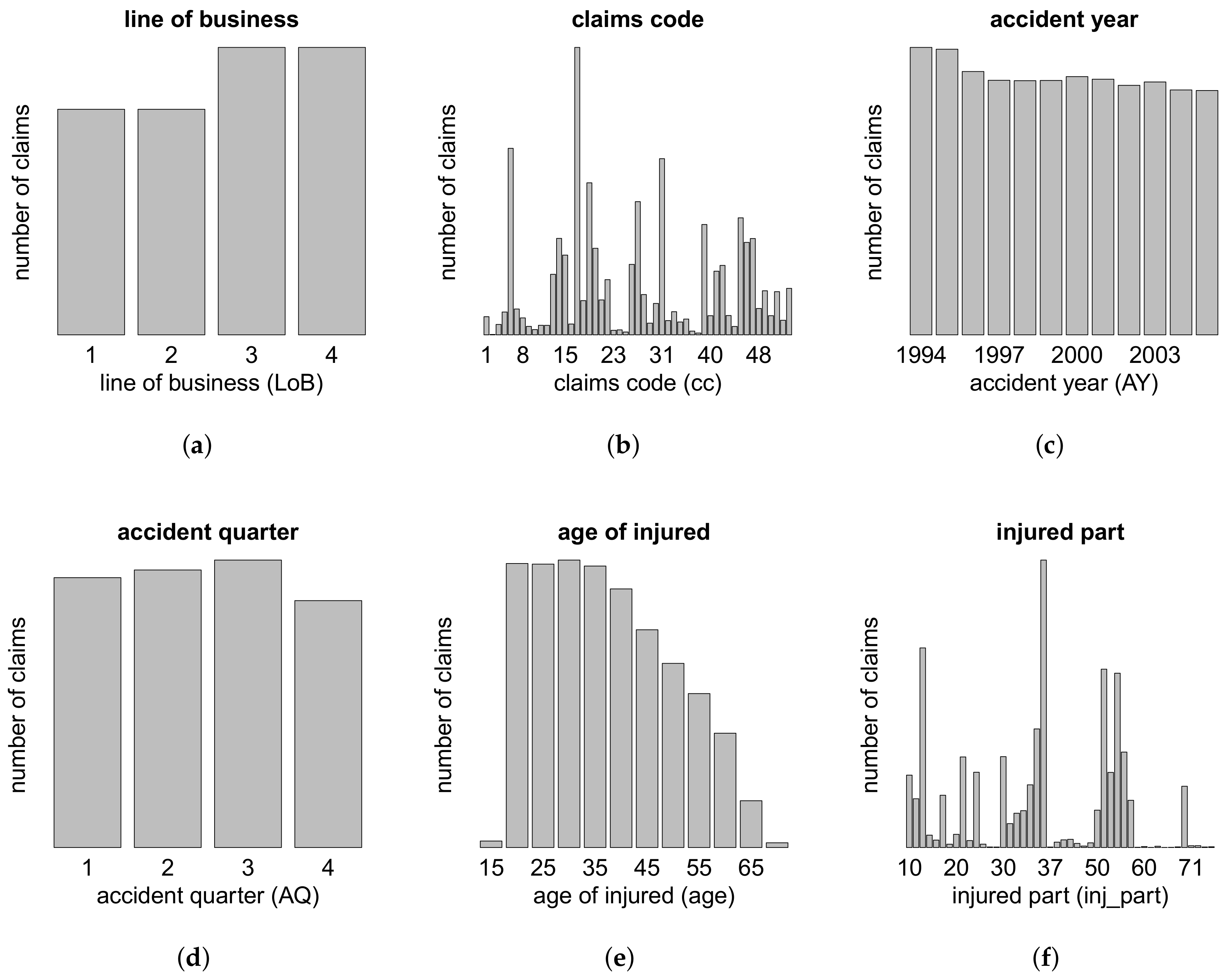
In this appendi we provide descriptive statistics of the data used to calibrate the individual claims history simulation machine. For confidentiality reasons, we can only show aggregate statistics of the claims portfolio, see Figure A1, Figure A2, Figure A3 and Figure A4 below.
Figure A1. Portfolio distributions w.r.t. the features (a) LoB; (b) cc; (c) AY; (d) AQ; (e) age and (f) inj_part.
Risks 06 00029 g0a1
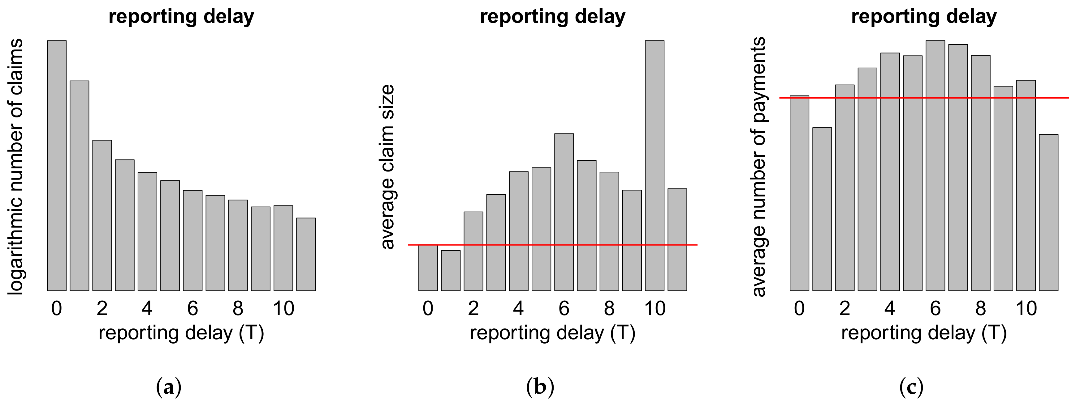
Figure A2. (a) Logarithmic number of claims; (b) average claim size and (c) average number of payments w.r.t. the reporting delay T; the red lines show the averages.
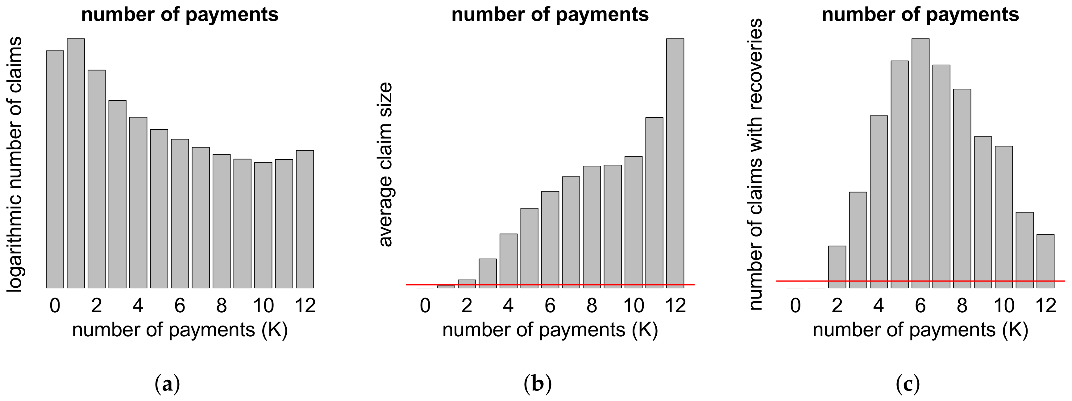
Risks 06 00029 g0a2
Figure A3. (a) Logarithmic number of claims; (b) average claim size and (c) number of claims with recoveries w.r.t. the number of payments K; the red lines show the averages.
Risks 06 00029 g0a3
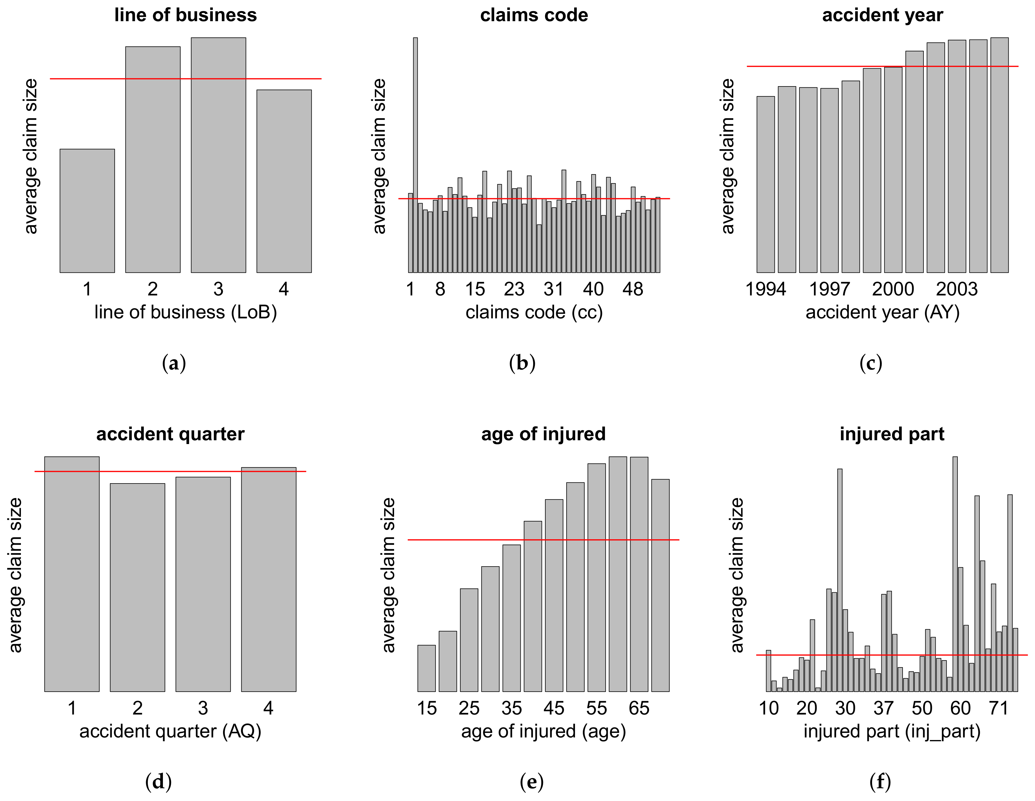
Figure A4. Average claim size w.r.t. the features (a) LoB; (b) cc; (c) AY; (d) AQ; (e) age and (f) inj_part; the red lines show the averages.
Risks 06 00029 g0a4

Appendix B. Procedure of Generating a Synthetic Portfolio

In order to use the stochastic simulation machine derived above, we require a portfolio of features x 1 , , x n X 1 , see (1). Therefore, we need an additional scenario generator that simulates reasonable synthetic portfolios. In this appendix we describe the design of our portfolio scenario generator which provides portfolios similar in structure to the original portfolio.
Our algorithm of synthetic portfolio generation uses the following input parameters:
  • V = totally expected number of claims;
  • ( p l ) 1 l 4 = categorical distribution for the allocation of the claims to the four lines of business;
  • ( r l ) 1 l 4 = growth parameters for the numbers of claims in the 12 accident years for each of the four lines of business.
In a first step, we use these parameters to simulate the total number of claims and allocate them to the lines of business LoB and the accident years AY. We start by simulating ( V l ) 1 l 4 according to
( V l ) 1 l 4 Multinomial V , ( p l ) 1 l 4 .
To determine the distribution of the claims among the 12 accident years within each line of business l = 1 , , 4 , we simulate ( X j ( l ) ) 1 l 4 , 2 j 12 from a normal distribution according to
X j ( l ) i . i . d . N ( r l , r l 2 ) .
Then, we define the weights W 1 ( l ) = 1 and
W j ( l ) = W j 1 ( l ) exp X j ( l ) ,
for all l = 1 , , 4 and j = 2 , , 12 . Finally, we set
V l , j = V l W j ( l ) j = 1 12 W j ( l ) ,
for all l = 1 , , 4 and j = 1 , , 12 , to be the expected number of claims in line of business l with accident year j. Conditionally given V = ( V 1 , 1 , V 1 , 2 , , V 4 , 12 ) , we simulate the number of claims N l , j in line of business l with accident year j from a Poisson distribution according to
N l , j | V ind . Poi ( V l , j ) ,
for all l = 1 , , 4 and j = 1 , , 12 . Note that we have E [ j = 1 12 N l , j ] = V p l , which justifies the above modeling choices.
After having simulated the number of claims N l , j for each line of business l and accident year j, we need to establish these claims with the remaining feature components cc, AQ, age and inj_part. This is achieved by choosing a multivariate distribution having a Gaussian copula and appropriate marginal densities. These densities and the covariance parameters of the Gaussian copula have been estimated from the real data. For the explicit parametrization, we refer to the R-function Feature.Generation in our simulation package.

Appendix C. Sensitivities of Selected Neural Networks

In this final appendix we consider 11 selected neural networks of our simulation machine and present the impact on the response variable of the respective most influential features. For each neural network considered, we use the corresponding calibration data set, fix a feature component—e.g., the accident quarter AQ—and vary its value over its entire domain—e.g., { 1 , , 4 } for the accident quarter AQ—to analyze the sensitivities in this feature component.
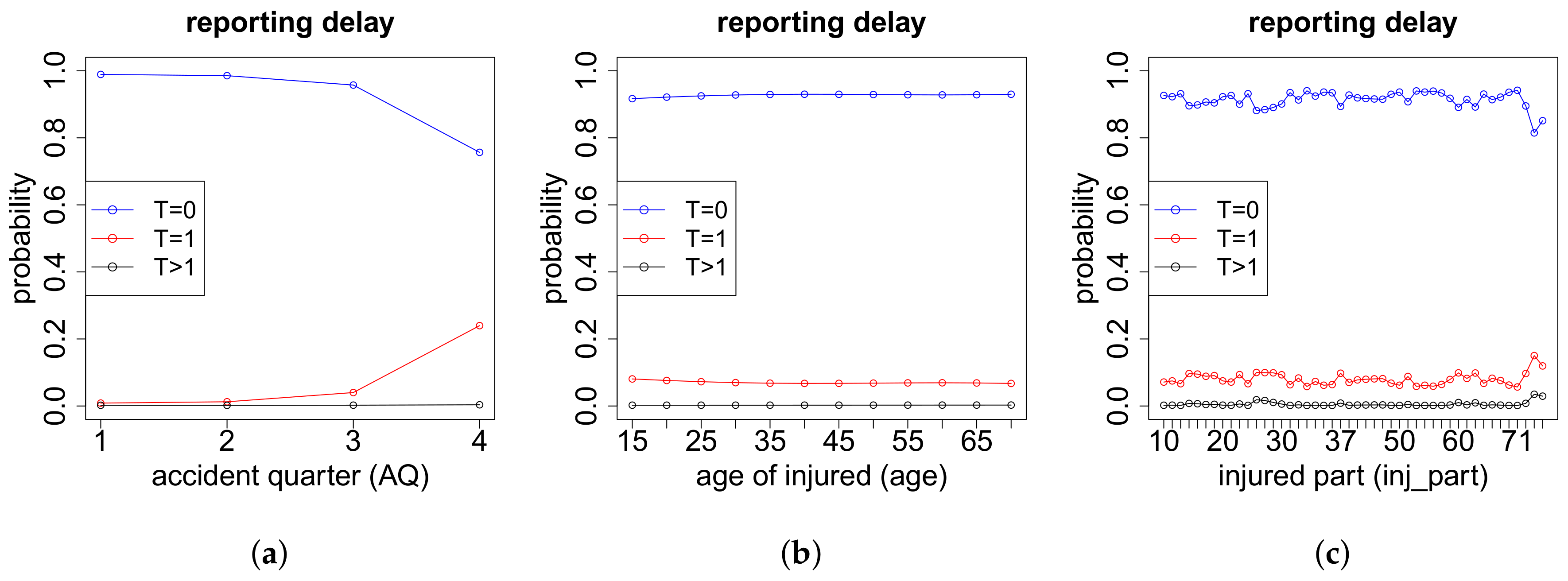
In Figure A5 we analyze the reporting delay T as a function of the features AQ, age and inj_part. Not surprisingly, the accident quarter has the biggest influence, because a claim occurring in December is likely to be reported only in the next accounting year.
Figure A5. Reporting delay T w.r.t. the features (a) AQ; (b) age and (c) inj_part.
Risks 06 00029 g0a5
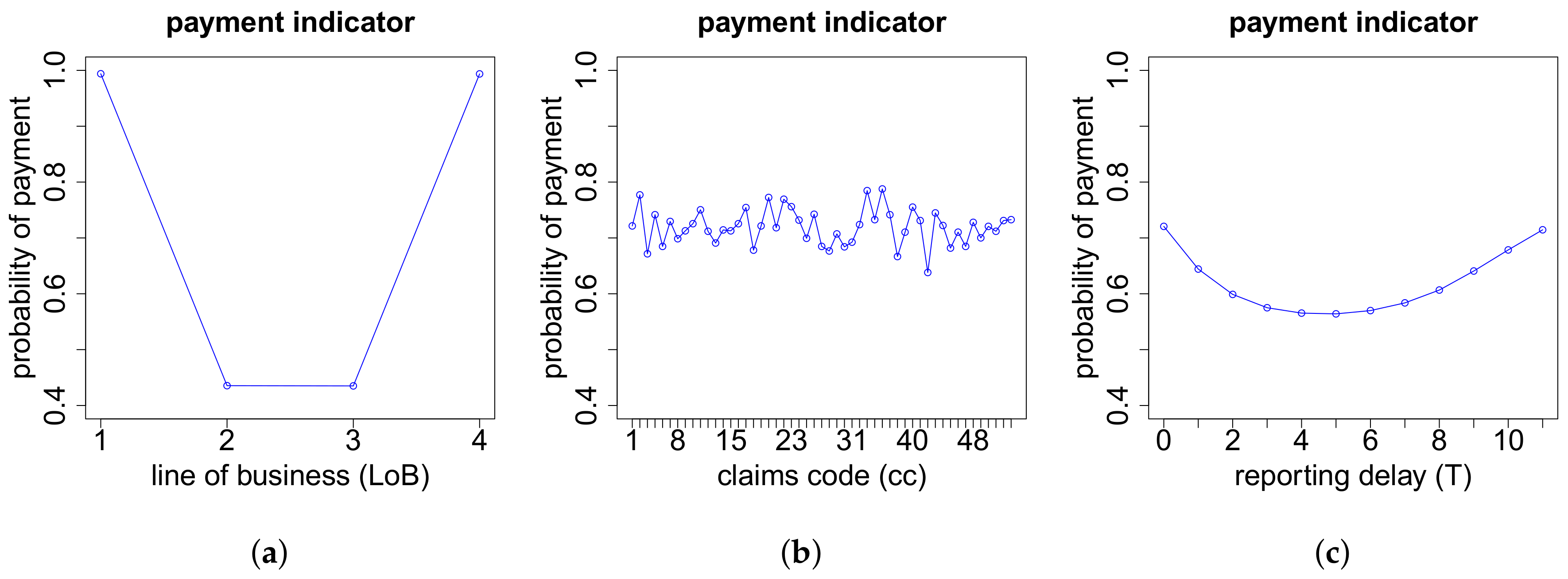
Figure A6 tells us that claims in lines of business one and four almost always have a payment. In contrast, we expect only roughly half of the claims in lines of business two and three to have a payment. Furthermore, the claims code cc causes some variation in the probability of having a payment, and claims with either a small or a large reporting delay T have a higher probability of having a payment than claims with a medium reporting delay.
Figure A6. Payment indicator Z w.r.t. the features (a) LoB; (b) cc and (c) reporting delay T.
Risks 06 00029 g0a6
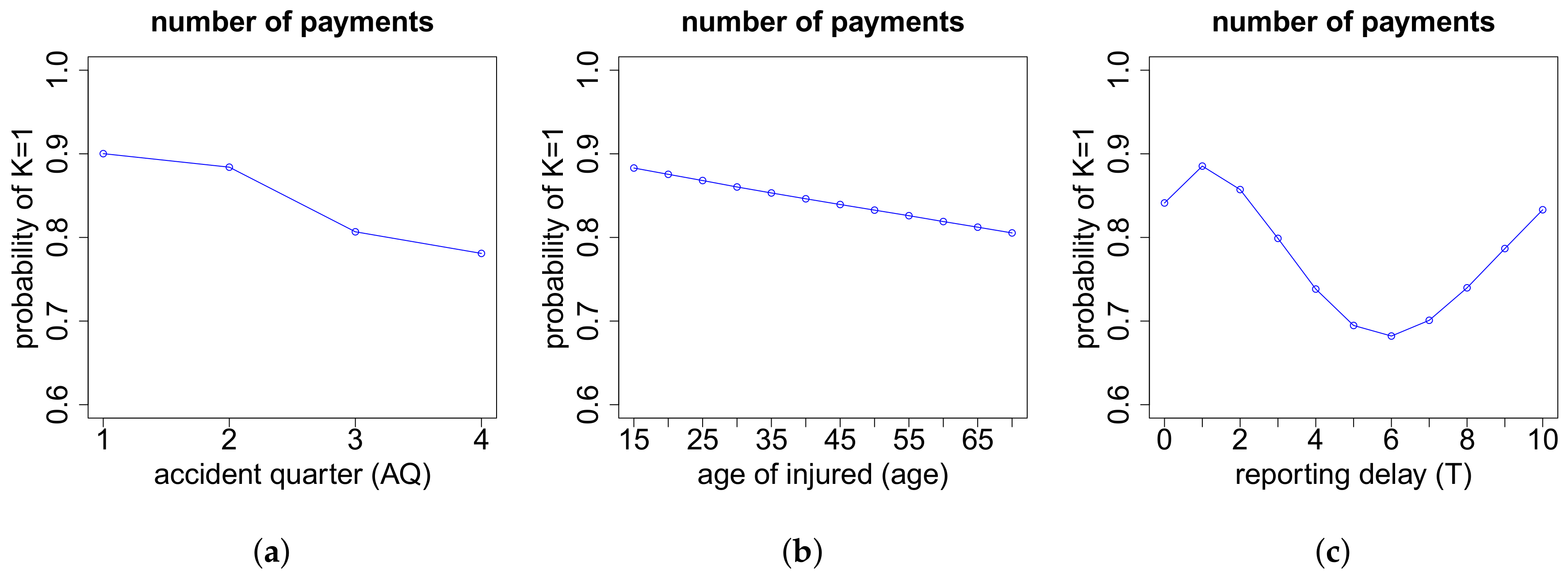
Recall that in determining the number of payments K, we use two neural networks, where in the first one we model whether we have K = 1 or K > 1 payments. According to Figure A7, claims that occur later in a year tend to have a higher probability of having more than one payment. The same holds true with increasing age of the injured. In passing from reporting delay T = 0 to T = 1 , the probability of having only one payment increases. But then we observe a sinus curve shape in that probability as a function of T.
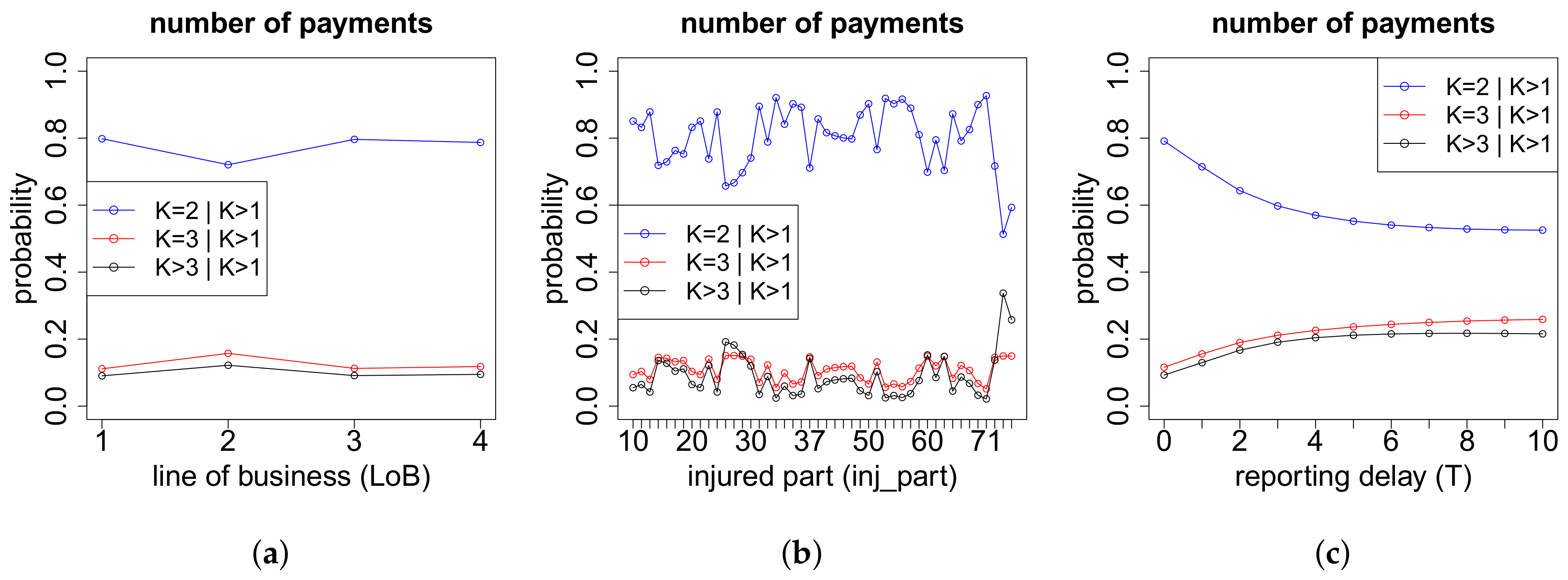
The second neural network used to determine the number of payments K models the distribution of K, conditioned on K > 1 . As we see in Figure A8, claims in line of business two tend to have more payments than claims in other lines of business, and both inj_part and reporting delay T heavily influence the number of payments.
Figure A7. Indicator whether we have K = 1 or K > 1 payments w.r.t. the features (a) AQ; (b) age and (c) reporting delay T.
Risks 06 00029 g0a7
Figure A8. Conditional distribution of the number of payments K, given K > 1 , w.r.t. the features (a) LoB; (b) inj_part and (c) reporting delay T.
Risks 06 00029 g0a8
In Figure A9 we present sensitivities for the expected total individual claim size Y on the log scale. The main drivers here are the line of business LoB and the number of payments K.
Figure A9. Total individual claim size Y (on log scale) w.r.t. the features (a) LoB; (b) reporting delay T and (c) number of payments K.
Risks 06 00029 g0a9
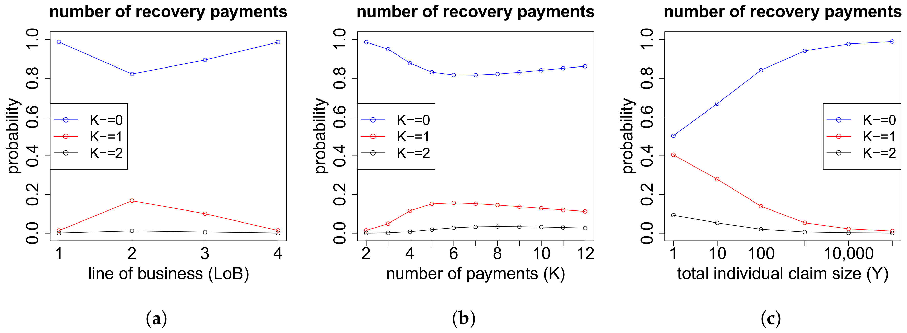
Figure A10 tells us that claims in lines of business one and four almost never have a recovery. Moreover, the probability of having at least one recovery payment first increases with the number of payments K but then slightly decreases again. Finally, up to 50 % of the claims with a small total individual claim size Y (of less than 10 CHF) have a recovery. This also comprises claims whose recovery is almost equal to the total gross claim amount, leading to a small net claim size. In general, the higher the total individual claim size, the less likely are recovery payments.
Figure A10. Number of recovery payments K w.r.t. the features (a) LoB; (b) number of payments K and (c) total individual claim size Y.
Risks 06 00029 g0a10
According to Figure A11, the total individual recovery Y is substantially higher for claims in lines of business two and three, compared to claims in lines of business one and four. Furthermore, if we have a recovery, then the higher the number of payments K and the total individual claim size Y, the higher also the recovery, where the increase w.r.t. the number of payments is decisively more pronounced.
Figure A11. Total individual recovery Y w.r.t. the features (a) LoB; (b) number of payments K and (c) total individual claim size Y.
Risks 06 00029 g0a11
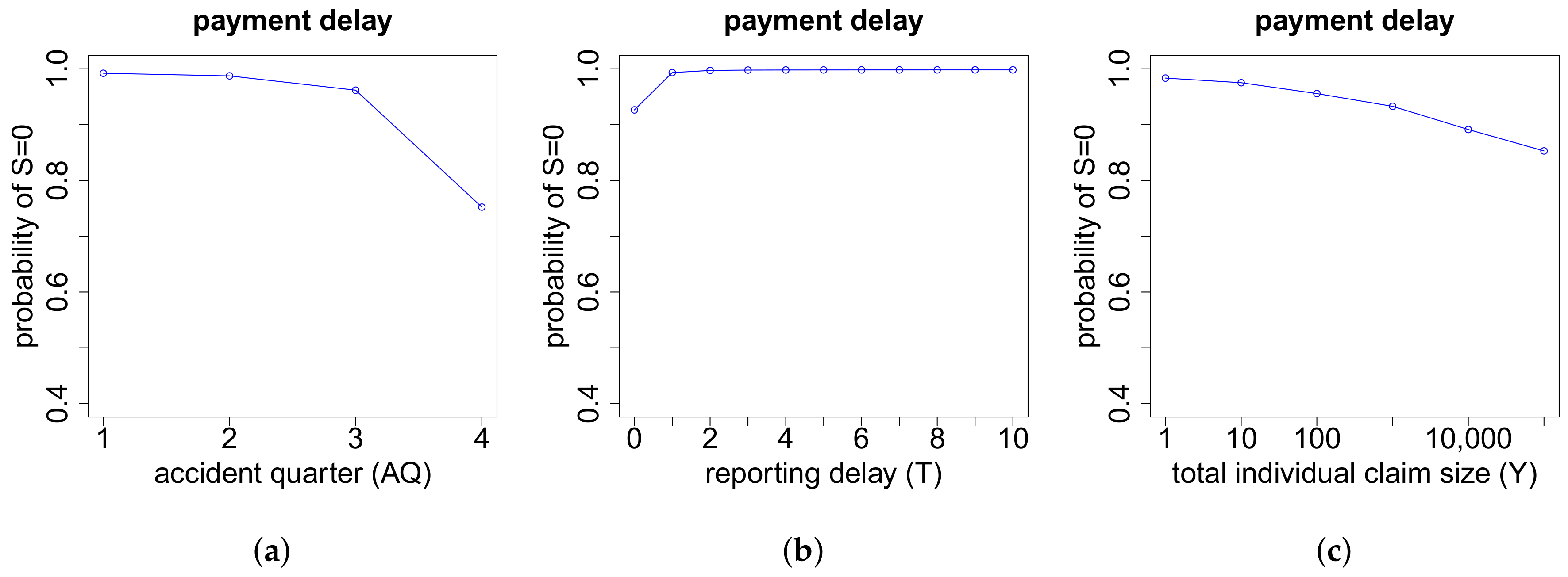
In determining the payment delay S for claims with exactly one payment, we use two neural networks. In the first one, we model whether S = 0 or S > 0 , and in the second one, we consider the conditional distribution of S, given S > 0 . Here we only present sensitivities for the first neural network. We observe, see Figure A12, that the probability of a payment delay equal to zero decreases with increasing accident quarter AQ and increasing total individual claim size Y. In particular, claims that occur in the last quarter of a year have a considerably higher probability of having a payment delay. This might be explained by claims for which the short time lag between the accident date and the end of the year only suffices for claims reporting but not for claims payments, leading to a payment delay. Finally, claims with a reporting delay T > 0 almost never have an additional payment delay.
Figure A12. Indicator whether we have payment delay S = 0 or S > 0 in the case of K = 1 payment w.r.t. the features (a) AQ; (b) reporting delay T and (c) total individual claim size Y.
Risks 06 00029 g0a12
As a representative of the neural networks that calculate the proportions with which the total gross claim amount Y + Y is distributed among the K + positive payments, we choose the one for K + = 6 . According to Figure A13, we see some monotonicity, but apart from that these proportions do not vary considerably. For claims which occur early during a year or have a high reporting delay T or a comparably small total individual claim size Y, the biggest proportion of the total gross claim amount is paid in the first (positive) payment.
Figure A13. Proportions P ( 1 ) , , P ( 6 ) of the total gross claim amount Y + Y paid in the K + = 6 positive payments w.r.t. the features (a) AQ; (b) reporting delay T and (c) total individual claim size Y.
Risks 06 00029 g0a13
According to Figure A14, in the case of K = 2 recovery payments, the proportion P of the total individual recovery Y that is paid in the first recovery payment varies substantially for the different values of the features cc and inj_part. We also observe that the higher the total individual recovery, the higher the proportion paid in the first recovery.
Figure A14. Proportion P of the total individual recovery Y paid in the first recovery payment in the case of K = 2 recovery payments w.r.t. the features (a) cc; (b) inj_part and (c) total individual recovery Y .
Risks 06 00029 g0a14
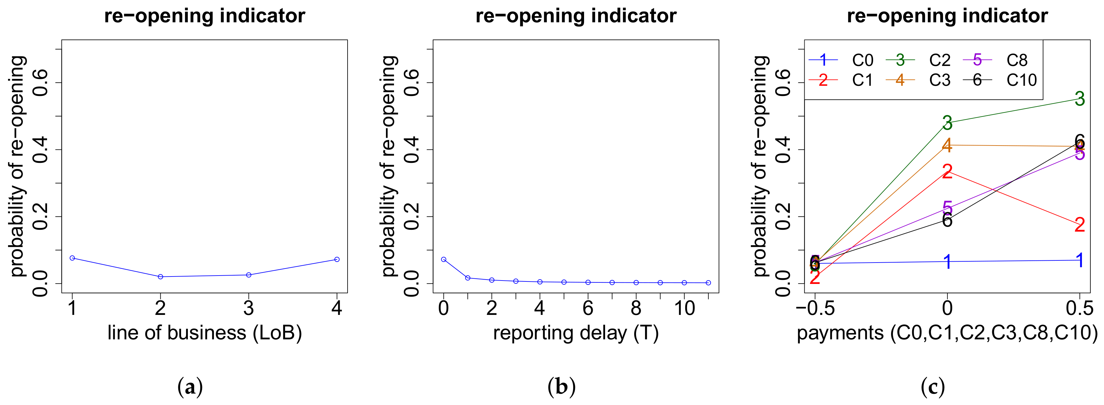
In Figure A15 we see that claims in lines of business one and four have a higher re-opening probability than claims in lines of business two and three. Moreover, the higher the reporting delay T of a claim, the lower the rate of reopening. Finally, the probability of re-opening heavily depends on the cash flow. In order to not overload the plot, we only show sensitivities w.r.t. the payments C ( 0 ) , C ( 1 ) , C ( 2 ) , C ( 3 ) , C ( 8 ) , C ( 10 ) . Recall that for this neural network, the yearly payments are coded with the values 1 2 , 0 and 1 2 , see (22). Summarizing, one can say that if we have a payment after the first development year, then the probability of re-opening is quite high.
Figure A15. Re-opening indicator V w.r.t. the features (a) LoB; (b) reporting delay T and (c) yearly payments C ( 0 ) , C ( 1 ) , C ( 2 ) , C ( 3 ) , C ( 8 ) , C ( 10 ) .
Risks 06 00029 g0a15

References

  1. Antonio, Katrien, and Richard Plat. 2014. Micro-Level Stochastic Loss Reserving for General Insurance. Scandinavian Actuarial Journal 7: 649–69. [Google Scholar] [CrossRef]
  2. Cybenko, George. 1989. Approximation by Superpositions of a Sigmoidal Function. Mathematics of Control, Signals, and Systems (MCSS) 2: 303–14. [Google Scholar] [CrossRef]
  3. Hiabu Munir, Carolin Margraff, Maria D. Martínez-Miranda, and Jens P. Nielsen. 2016. The Link between Classical Reserving and Granular Reserving through Double Chain-Ladder and its Extensions. British Actuarial Journal 21: 97–116. [Google Scholar] [CrossRef]
  4. Hornik, Kurt, Maxwell Stinchcombe, and Halbert White. 1989. Multilayer Feedforward Networks are Universal Approximators. Neural Networks 2: 359–66. [Google Scholar] [CrossRef]
  5. Jessen, Anders H., Thomas Mikosch, and Gennady Samorodnitsky. 2011. Prediction of Outstanding Payments in a Poisson Cluster Model. Scandinavian Actuarial Journal 3: 214–37. [Google Scholar] [CrossRef]
  6. Mack, Thomas. 1993. Distribution-Free Calculation of the Standard Error of Chain Ladder Reserve Estimates. ASTIN Bulletin 23: 213–25. [Google Scholar] [CrossRef]
  7. Martínez-Miranda, Maria D., Jens P. Nielsen, Richard J. Verrall, and Mario V. Wüthrich. 2015. The Link between Classical Reserving and Granular Reserving through Double Chain-Ladder and its Extensions. Scandinavian Actuarial Journal 5: 383–405. [Google Scholar]
  8. Pigeon, Mathieu, Katrien Antonio, and Michel Denuit. 2013. Individual Loss Reserving with the Multivariate Skew Normal Framework. ASTIN Bulletin 43: 399–428. [Google Scholar] [CrossRef]
  9. Rumelhart, David E., Geoffrey E. Hinton, and Ronald J. Williams. 1986. Learning Representations by Back- Propagating Errors. Nature 323: 533–36. [Google Scholar] [CrossRef]
  10. Taylor, Greg, Gráinne McGuire, and James Sullivan. 2008. Individual Claim Loss Reserving Conditioned by Case Estimates. Annals of Actuarial Science 3: 215–56. [Google Scholar] [CrossRef]
  11. Verrall, Richard J., and Mario V. Wüthrich. 2016. Understanding Reporting Delay in General Insurance. Risks 4: 25. [Google Scholar] [CrossRef]
  12. Werbos, Paul J. 1982. Applications of Advances in Nonlinear Sensitivity Analysis. In System Modeling and Optimization. Paper Presented at the 10th IFIP Conference, New York City, NY, USA, 31 August–4 September 1981. Edited by Rudolf F. Drenick and Frank Kozin. Berlin and Heidelberg: Springer, pp. 762–70. [Google Scholar]
  13. Wüthrich, Mario V. 2018. Machine Learning in Individual Claims Reserving. To appear in Scandinavian Actuarial Journal 25: 1–16. [Google Scholar]
  14. Wüthrich, Mario V. 2018. Neural Networks Applied to Chain-Ladder Reserving. SSRN Manuscript. [Google Scholar] [CrossRef]
Figure 1. Deep neural network with two hidden layers: the first column (blue circles) illustrates the d = 6 dimensional feature vector x (input layer), the second column gives the first hidden layer with q 1 = 11 neurons, the third column gives the second hidden layer with q 2 = 15 neurons and the fourth column gives the output layer (red circle) with 12 neurons.
Risks 06 00029 g001
Table 1. Number of possible and allowed distribution patterns for K = 3 , , 10 payments.
Number of Payments K345678910
number of possible patterns | A | 22049579292479249522066
number of allowed patterns | A ˜ | 1518172117202624
percentage of claims covered 91 % 83 % 73 % 70 % 62 % 61 % 64 % 76 %
Table 2. Triangle of reported claims of the real data.
AccidentReporting Delay T
Year AY01234567891011
1994861,89959,0561540460230154845650283212
1995850,29764,73315685622161249462443432
1996781,87561,465174241425215376623822
1997756,14759,2691466496210147544840
1998753,55260,24916605302481369844
1999754,99259,690162546820810068
2000766,68461,120127432013688
2001758,44361,449102428690
2002745,12555,246876200
2003757,84353,272956
2004733,78551,742
2005730,978
Table 3. Triangle of reported claims of the simulated data.
AccidentReporting Delay T
Year AY01234567891011
1994860,33760,14318375532561551017057353621
1995851,87762,92417764992631648058522936
1996783,00660,511155747718212287495339
1997756,01559,5561434399169129774242
1998752,45461,91314223801641006537
1999753,63561,552127936215311649
2000768,18059,636121533815071
2001759,50160,1311124304132
2002744,47855,5771012270
2003757,63553,352937
2004732,88452,586
2005731,357
Table 4. Triangle of cumulative claims payments (in 10,000 CHF) of the real data.
AccidentDevelopment Delay j
Year AY01234567891011
199478,433120,396130,167134,749137,143138,798139,994141,052142,106142,913143,652144,247
199579,372124,532135,488140,338143,145144,859146,408147,624148,735149,686150,578
199671,398113,335123,336128,052130,779132,692134,175135,359136,381137,311
199768,600107,716117,556122,331125,304127,477129,037130,171131,216
199868,055109,906120,706126,443129,727131,998133,745135,176
199971,989114,344127,311134,174138,075140,614142,530
200072,225118,418131,615138,216142,024144,450
200174,891126,244141,008147,923151,917
200278,167129,105143,731150,560
200382,668134,010148,161
200480,630130,390
200582,015
Table 5. Triangle of cumulative claims payments (in 10,000 CHF) of the simulated data.
AccidentDevelopment Delay j
Year AY01234567891011
199480,491117,807129,673135,331138,591140,745142,268143,394144,344145,090145,694146,076
199579,170116,943129,313135,330138,785141,079142,743144,045145,115146,002146,760
199671,675107,228119,578125,407128,771131,009132,566133,718134,657135,472
199768,857104,291116,406122,177125,495127,662129,194130,388131,270
199867,418103,415116,194122,262125,673127,877129,452130,588
199969,308107,587121,381127,930131,534133,924135,502
200073,359113,266127,878134,804138,806141,431
200173,338115,626131,197138,481142,591
200274,887117,602133,850141,539
200381,921127,461144,444
200481,394128,864
200586,837
Table 6. Chain-ladder predicted numbers of incurred but not yet reported (IBNYR) claims and Mack’s msep for the real and the simulated data.
AccidentCL Predicted msep in %CL Predicted msep in %
Year AYIBNYR Claims IBNYR Claims
Real DataSimulated Data
19940 0
19951200.0%2100.0%
19964000.4%5200.4%
19976558.4%8278.6%
199810576.2%12996.6%
1999156106.1%178147.7%
2000235198.0%255218.3%
2001357329.0%370359.4%
20025366512.2%535539.9%
200394413514.3%9259510.2%
2004220133015.0%217026512.2%
200557,73435426.1%57,78934105.9%
total62,38535655.7%62,50634255.5%
Table 7. Chain-ladder reserves for claims payments (in 10,000 CHF) and Mack’s msep for the real and the simulated data.
AccidentCL Reserves msep in %CL Reserves msep in %
Year AY
Real DataSimulated Data
19940 0
199562411718.8%38510928.2%
1996133714610.9%99116116.2%
199721121688.0%172317910.4%
199832241775.5%26361877.1%
199946862595.5%39432095.3%
200064763946.1%58262303.9%
200192755996.5%88462903.4%
200213,0498896.8%12,4894213.4%
200319,97314217.1%20,8178374.0%
200432,53223947.4%36,64720505.6%
200582,70650396.1%84,17549685.9%
total175,99462753.6%178,07657323.2%