Bayesian Joint Estimation of the Hurst Parameter and Volatility with Applications to Fractional Option Pricing

Abstract

Fractional Brownian motion has been widely used in financial modeling to capture long-range dependence and persistent behavior in asset dynamics. In the fractional Black–Scholes framework, accurate estimation of the Hurst parameter is essential because estimation uncertainty can directly affect option pricing. In this paper, we propose a Bayesian framework for joint inference on the Hurst parameter and volatility in fractional stochastic differential equation models. Unlike approaches based solely on point estimation, the proposed framework propagates posterior uncertainty directly into option pricing distributions under the fractional Black–Scholes model. Simulation studies are conducted across multiple values of the Hurst parameter and sample sizes to evaluate estimation accuracy, posterior coverage, and pricing uncertainty. The results demonstrate stable posterior inference and coherent uncertainty quantification for both model parameters and option prices. The methodology is further illustrated using WTI crude oil and natural gas data under different market regimes. The empirical analysis indicates that differences in market behavior are driven primarily by changes in volatility rather than strong long-range dependence, while posterior option price distributions exhibit substantial variation in pricing uncertainty across regimes. These findings highlight the importance of incorporating joint parameter uncertainty into fractional financial models and demonstrate the practical value of Bayesian methods for option pricing.

1. Introduction

The pricing of financial derivatives remains a central topic in mathematical finance, with the Black–Scholes model representing a fundamental breakthrough in the field (Black and Scholes 1973; Merton 1973). By modeling asset prices through geometric Brownian motion under a no-arbitrage framework, the model provides a closed-form solution for European option pricing and has become a cornerstone of modern financial theory. Despite its widespread use, empirical studies have shown that financial time series often exhibit features that are inconsistent with the model assumptions, including long-range dependence, volatility clustering, and heavy-tailed return distributions.

Fractional Brownian motion directly addresses these shortcomings by introducing memory into the stochastic dynamics of asset prices. Fractional Brownian motion (fBm) was formally introduced by Mandelbrot and Van Ness (1968), who defined it as a generalization of standard Brownian motion with stationary, correlated increments. Its relevance to financial time series—particularly the presence of long-range dependence—was subsequently argued by Mandelbrot (1971). Fractional Brownian motion incorporates a Hurst parameter that characterizes long-range ependence in stochastic processes. In this framework, the Hurst parameter $H\in (0,1)$ governs the degree of dependence in the process, while $\sigma >0$ denotes the volatility. In particular, when the Hurst parameter exceeds one-half, the process exhibits persistence, reflecting the tendency of financial returns to display long memory. This has led to the development of fractional Black–Scholes models, which extend the classical framework by incorporating memory effects and providing a more flexible representation of asset dynamics (Biagini et al. 2008). More recent developments in financial modeling have also emphasized rough volatility and fractional dynamics as realistic representations of market behavior, particularly at high frequencies (Bennedsen et al. 2022; Gatheral et al. 2018). Several studies have proposed explicit formulations of such models based on fractional Brownian motion, illustrating how the Hurst parameter influences option pricing and volatility dynamics (Comte and Renault 1998; Hu and Øksendal 2003; Njomen and Djeutcha 2019). Early studies also investigated option pricing in markets driven by fractional Brownian motion and demonstrated the potential impact of long-range dependence on derivative valuation (Necula 2002). Notwithstanding these advances, the problem of jointly estimating the Hurst parameter H and the volatility $\sigma$ within a unified statistical framework has received comparatively less attention in the context of uncertainty quantification for fractional option pricing. Despite these advances, reliable inference remains challenging because the Hurst parameter and volatility must be estimated simultaneously while accounting for their joint uncertainty. Although fractional models provide a more realistic description of asset dynamics, many existing approaches rely primarily on point estimates or separate marginal intervals, which may fail to capture the dependence between these parameters. Consequently, estimation uncertainty may be underrepresented, potentially affecting option valuation, hedging strategies, risk management, and portfolio allocation. As a result, estimation error can be misrepresented, potentially leading to inaccurate assessments in financial applications. From a practical perspective, these challenges are especially important in decision-making, where even small inaccuracies can lead to meaningful differences in option values and affect hedging strategies, risk management, and portfolio allocation. Accurate estimation of the Hurst parameter has been a central challenge in the application of fractional models to financial data. The statistical theory of long-range dependence has been extensively developed in both Gaussian and non-Gaussian settings, with applications across telecommunications, hydrology, economics, and finance (Beran 1994; Doukhan et al. 2003; Embrechts and Maejima 2002; Samorodnitsky and Taqqu 1994). These developments have established the Hurst parameter as a key measure of persistence and dependence in stochastic processes.

A wide range of methods has been proposed for estimating long-range dependence, each with different trade-offs between bias, efficiency, and computational complexity. Early work by Beran (1994) provided a systematic treatment of statistical methods for long-memory processes, while subsequent studies highlighted the sensitivity of classical estimators to short-range dependence and finite-sample effects (Taqqu et al. 1995). Semi-parametric approaches, such as log-periodogram regression and local Whittle estimation, have been widely used because of their attractive asymptotic properties, although they often require relatively large sample sizes to achieve reliable performance (Hurvich et al. 1998; Robinson 1995). Alternative approaches include wavelet-based estimators, which exploit the scale invariance of fractional processes and have been shown to improve estimation accuracy in certain settings (Abry and Veitch 1998; Bardet et al. 2000). More recently, bias-corrected estimation procedures have also been proposed to improve finite-sample performance in fractional option-pricing applications (Pramanik et al. 2024; Sagor et al. 2025). A broader overview of commonly used Hurst exponent estimation procedures and their practical characteristics is provided by Zhang et al. (2024).

Despite these advances, reliable inference remains challenging because the Hurst parameter and volatility must be estimated simultaneously while accounting for their joint uncertainty. Although fractional models provide a more realistic description of asset dynamics, many existing approaches rely primarily on point estimates or separate marginal intervals, which may fail to capture the dependence between these parameters. Consequently, estimation uncertainty may be underrepresented, potentially affecting option valuation, hedging strategies, risk management, and portfolio allocation.

Bayesian approaches have been developed as a flexible framework for inference in long-memory and fractional stochastic processes (Beskos et al. 2015; Chaim and Laurini 2024; Chen et al. 2017; Dlask et al. 2017; Makarava and Holschneider 2012; Tsionas 2021; Weron 2002). For example, Makarava and Holschneider (2012) proposed Bayesian estimation of the Hurst parameter for fractional Brownian motion, Beskos et al. (2015) developed Bayesian inference for stochastic differential equations driven by fractional Brownian motion, Dlask et al. (2017) investigated Bayesian estimation of the Hurst exponent through posterior summaries, Jacquier et al. (1994) introduced a seminal Bayesian framework for stochastic volatility models, Tsionas (2021) studied Bayesian models with static and dynamic Hurst parameters under stochastic volatility, and Chaim and Laurini (2024) developed Bayesian inference for long-memory stochastic volatility models. Despite these advances, relatively less attention has been devoted to characterizing the joint posterior dependence between the Hurst parameter and volatility, evaluating multivariate highest-density regions (HDRs), and propagating the resulting joint posterior uncertainty into fractional option pricing. These gaps motivate the unified Bayesian framework proposed in this paper, which explicitly links joint parameter inference with uncertainty quantification for fractional option pricing.

At the same time, maximum likelihood and the method of moments estimators are known to exhibit systematic bias when applied to fractional stochastic differential equation models, particularly for values of the Hurst parameter away from 0.5. This issue has been documented in both parametric and moment-based settings (Pramanik et al. 2024; Sagor et al. 2025), where it is shown that both maximum likelihood and method of moments estimators require bias correction for reliable practical use.

These limitations motivate Bayesian inference, which provides a coherent framework for combining prior information with observed data to obtain posterior distributions over the model parameters (Murphy 2012). A key advantage of this framework is its ability to capture posterior dependence between parameters rather than treating them independently. In this context, joint highest-density regions (HDRs) offer a principled method for summarizing uncertainty in a multidimensional setting, providing a more accurate representation than separate marginal intervals.

Motivated by these considerations, this paper develops a Bayesian framework for simultaneous inference on the Hurst parameter and volatility within a fractional Gaussian noise framework. Using a simulation-based approach, we construct empirical joint highest-density regions for $(H,\sigma )$ and evaluate their repeated-sampling performance. The results reveal strong posterior dependence between parameters and highlight the limitations of marginal interval-based inference.

To assess the practical implications of parameter uncertainty, posterior samples are propagated through the fractional Black–Scholes pricing formula to obtain distributions of option prices. This approach allows for the construction of credible intervals that reflect joint parameter uncertainty, providing a more informative basis for decision-making compared to traditional point estimates.

The principal contribution of this paper is therefore not the development of a new estimation algorithm, but rather a unified Bayesian inference framework that explicitly links parameter estimation, joint uncertainty quantification, and fractional option pricing. Specifically, the proposed framework (i) jointly estimates the Hurst parameter and volatility, (ii) characterizes their posterior dependence through joint highest-density regions (HDRs), (iii) evaluates the repeated-sampling performance of these regions through simulation, and (iv) propagates the resulting joint posterior distribution through the fractional Black–Scholes pricing model to quantify option-pricing uncertainty. Unlike approaches based solely on point estimates or on separate marginal credible intervals, the proposed framework preserves parameter dependence, providing a more comprehensive probabilistic assessment of uncertainty in fractional option pricing.

The remainder of the paper is organized as follows. Section 2 presents the fractional Black–Scholes framework and the Bayesian methodology used to jointly estimate H and $\sigma$, including prior specification, posterior computation, and the construction of joint highest-density regions. Section 3 reports a simulation study evaluating the performance of the proposed estimators, with emphasis on coverage, posterior dependence, and estimation accuracy. Section 4 provides an empirical application in which posterior parameter draws are propagated through the fractional Black–Scholes pricing formula to quantify option pricing uncertainty. Section 5 concludes the paper and discusses limitations and directions for future research.

2. Methodology

This section describes the simulation framework used to study Bayesian estimation of the Hurst parameter H and the scale parameter $\sigma$ under fractional Gaussian noise (fGn). We construct joint highest-density regions (HDRs) for $(H,\sigma )$ and assess repeated-sampling coverage with respect to the true pair $(H_c,{\sigma }_0)$.

2.1. Data-Generating Mechanism

Let $d={(d_1,\dots ,d_n)}^{\top }$ denote an observed fGn sample of length n. For a fixed Hurst parameter $H\in (1/2,1)$, the lag-k autocovariance of unit-variance fGn is

$${\rho }_H\left(k\right)={\displaystyle \frac{1}{2}}\left({|k+1|}^{2H}-{2\left|k\right|}^{2H}+{|k-1|}^{2H}\right),k=0,1,2,\dots .$$

(1)

Since ${\rho }_H\left(0\right)=1$, ${\rho }_H\left(k\right)$ also equals the lag-k autocorrelation, as derived from fractional Brownian motion (Beran 1994; Mandelbrot and Van Ness 1968).

Using (1), the $n\times n$ Toeplitz correlation matrix $R\left(H\right)$ is defined by

$$R\left(H\right)=\left(\begin{array}{cccc}{\rho }_H\left(0\right)& {\rho }_H\left(1\right)& \cdots & {\rho }_H(n-1)\\ {\rho }_H\left(1\right)& {\rho }_H\left(0\right)& \cdots & {\rho }_H(n-2)\\ ⋮& ⋮& \ddots & ⋮\\ {\rho }_H(n-1)& {\rho }_H(n-2)& \cdots & {\rho }_H\left(0\right)\end{array}\right).$$

(2)

This Toeplitz structure is standard in long-memory Gaussian processes (Beran 1994) and provides the basis for data generation in our simulation study. For fixed true values $({\mu }_0,{\sigma }_0,H_c)$, the simulated sample is generated from the corresponding Gaussian model using this covariance structure.

$$d\sim N\left({\mu }_0{\mathbf{1}}_n,{\sigma }_0^{2}R\left(H_c\right)\right),$$

(3)

where ${\mathbf{1}}_n$ denotes the n-vector of ones.

To simulate exactly from (3), we compute the Cholesky factorization

$$R\left(H_c\right)=U^{\top }U,$$

(4)

generate $z\sim N(0,I_n)$, and set

$$d={\mu }_0{\mathbf{1}}_n+{\sigma }_0{U}^{\top }z.$$

(5)

This yields an exact Gaussian sample with mean ${\mu }_0{\mathbf{1}}_n$ and covariance ${\sigma }_0^{2}R\left(H_c\right)$. Cholesky factorization provides a numerically stable and computationally efficient approach for simulating Gaussian vectors with positive-definite covariance matrices (Golub and Van Loan 2013). The Gaussian fractional Gaussian noise (fGn) likelihood adopted in this paper is motivated by the assumed fractional Black–Scholes model. Specifically, under the fractional Black–Scholes dynamics, the logarithm of the asset price is driven by fractional Brownian motion, whose discrete-time increments form a fractional Gaussian noise process. Consequently, the covariance structure of the observed log returns is determined by the Hurst parameter H and scaled by the volatility parameter $\sigma$, leading naturally to the Gaussian fGn likelihood used for inference. The posterior distribution of $(H,\sigma )$ obtained from this likelihood therefore represents inference on the same parameters that govern the assumed fractional Black–Scholes dynamics and is subsequently propagated through the pricing formula under the assumption that the observed log returns are adequately represented by the corresponding fGn model.

2.2. Bayesian Model Specification

Conditional on $(\mu ,\sigma ,H)$, the data are modeled as

$$d\mid \mu ,\sigma ,H\sim N\left(\mu {\mathbf{1}}_n,{\sigma }^{2}R\left(H\right)\right),$$

(6)

with $H\in (H_L,H_U)$, where in our implementation $H_L=0.5$ and $H_U=1$.

The prior distributions are chosen as

$$\begin{array}{cc}\hfill \mu & \sim N({\mu }_0^{*},{\tau }_{\mu }^2),\hfill \end{array}$$

(7)

$$\begin{array}{cc}\hfill \sigma & \sim \mathrm{Lognormal}(m_{\sigma },s_{\sigma }^2),\hfill \end{array}$$

(8)

$$\begin{array}{cc}\hfill H& \sim \mathrm{Uniform}(H_L,H_U),\hfill \end{array}$$

(9)

where ${\mu }_0^{*}$, ${\tau }_{\mu }^2$, $m_{\sigma }$, and $s_{\sigma }^2$ are fixed hyperparameters. The Normal prior for $\mu$ is weakly informative and reflects prior uncertainty about the mean return while allowing the data to dominate the posterior inference for the sample sizes considered (Gelman et al. 2013; Murphy 2012).

The Lognormal prior for $\sigma$ is adopted because volatility is strictly positive and the Lognormal distribution naturally satisfies this constraint while providing a flexible, weakly informative prior over a broad range of plausible values. Weakly informative priors for scale parameters are commonly recommended to regularize estimation without overly influencing posterior inference (Gelman 2006; Gelman et al. 2013). Although other positive priors, such as the Half-Normal, Half-Cauchy, and Inverse-Gamma distributions, are widely used in Bayesian analysis, the Lognormal prior provides a simple and interpretable specification of volatility in the present framework. The impact of alternative prior choices is investigated through a prior sensitivity analysis in the empirical application presented in Section 4.

The Uniform prior on $H\in (0.5,1)$ reflects the absence of strong prior information while restricting inference to the admissible parameter space of the fractional Brownian motion model, where $H>0.5$ corresponds to persistent dependence. This prior assigns equal probability to all admissible values and therefore does not favor any particular degree of long-range dependence (Beran 1994; Mandelbrot and Van Ness 1968).

Hence, the posterior density is

$$\pi (\mu ,\sigma ,H\mid d)\propto L(d\mid \mu ,\sigma ,H)\pi \left(\mu \right)\pi \left(\sigma \right)\pi \left(H\right),$$

(10)

where $L(d\mid \mu ,\sigma ,H)$ is the multivariate normal likelihood induced by (6).

2.3. Posterior Computation

Under (6), the log-likelihood is

$$\begin{array}{cc}logL(d\mid \mu ,\sigma ,H)=-{\displaystyle \frac{1}{2}}[\hfill & nlog\left(2\pi \right)+nlog\left({\sigma }^2\right)+log\left|R\left(H\right)\right|\hfill \\ \hfill & +{\displaystyle \frac{1}{{\sigma }^2}}{(d-\mu {\mathbf{1}}_n)}^{\top }R{\left(H\right)}^{-1}(d-\mu {\mathbf{1}}_n)],\hfill \end{array}$$

(11)

which follows from the multivariate Gaussian likelihood (Beran 1994). To evaluate the log-likelihood efficiently, we use the Cholesky factorization

$$R\left(H\right)=C{\left(H\right)}^{\top }C\left(H\right),$$

(12)

so that

$$log\left|R\left(H\right)\right|=2{\displaystyle \sum _{i=1}^n}log{C}_{ii}\left(H\right),$$

(13)

and the quadratic form is evaluated through triangular solves rather than direct matrix inversion, which improves numerical stability and computational efficiency.

The dominant computational cost in evaluating the log-likelihood arises from the Cholesky factorization of the covariance matrix $R\left(H\right)$, which requires $\mathcal{O}\left(n^3\right)$ operations. Once the factorization is obtained, the log-determinant and quadratic form are computed using forward and backward triangular substitutions with computational cost $\mathcal{O}\left(n^2\right)$, thereby avoiding explicit matrix inversion. To further improve numerical stability, a small positive diagonal regularization term is added to $R\left(H\right)$ prior to the Cholesky factorization. This regularization mitigates numerical ill-conditioning, while the Cholesky factorization and triangular solves provide a stable and efficient means of evaluating the Gaussian log-likelihood without forming the inverse covariance matrix (Golub and Van Loan 2013; Higham 2002).

Combining (11) with the priors (7)–(), the log-posterior is

$$log\pi (\mu ,\sigma ,H\mid d)=logL(d\mid \mu ,\sigma ,H)+log\pi \left(\mu \right)+log\pi \left(\sigma \right)+log\pi \left(H\right)+\mathrm{constant}.$$

(14)

2.4. Bayesian Implementation

To facilitate efficient MCMC sampling and avoid boundary issues, we work with transformed parameters (Chopin and Papaspiliopoulos 2020). For the volatility parameter $\sigma >0$, we define $\eta =log\sigma$. For the Hurst parameter $H\in (H_L,H_U)$, we apply a logit transformation

$$z_H=log\left({\displaystyle \frac{H-H_L}{H_U-H_L-(H-H_L)}}\right),$$

(15)

which maps H to the real line. The corresponding Jacobian adjustments are included in the posterior target density.

Posterior inference is carried out using a Metropolis-within-Gibbs scheme with random-walk proposals (Chopin and Papaspiliopoulos 2020). To improve sampling efficiency, we incorporate a joint block update for $(H,\sigma )$, motivated by their strong posterior dependence. The proposal covariance is estimated from a preliminary pilot run and used to construct a bivariate Gaussian random-walk proposal aligned with the posterior geometry. This substantially improves mixing in regions of high posterior curvature.

All computations were performed using R version 4.5.1 (R Foundation for Statistical Computing, Vienna, Austria). Trace plots, effective sample sizes, autocorrelation functions, and Geweke diagnostic statistics were obtained using the coda package version 0.19.4.1 in R.

To assess convergence and sampling efficiency, standard MCMC diagnostic tools were employed (Kass et al. 1998). Trace plots were visually inspected to verify adequate mixing and the absence of systematic trends. Effective sample sizes (ESS), autocorrelation functions (ACF), Geweke diagnostic statistics (Geweke 1992), and acceptance rates for both the individual and block Metropolis updates were also examined. The trace plots showed stable mixing without noticeable trends; the Geweke statistics were within the commonly accepted convergence range; and the effective sample sizes indicated adequate sampling efficiency. Representative diagnostic plots and summary statistics are presented in the empirical application section.

2.5. Joint Highest-Density Region Coverage

Following the posterior sampling step, we evaluate the transformed posterior log-density at each draw as

$$h^{\left(m\right)}=log\tilde{\pi }({\mu }^{\left(m\right)},{\eta }^{\left(m\right)},z_H^{\left(m\right)}\mid d),$$

(16)

which is used to construct the joint highest-density regions.

The transformed posterior log-density is evaluated at each retained posterior draw $m=1,\dots ,M$, producing a set of posterior heights ${\left\{h^{\left(m\right)}\right\}}_{m=1}^M$. These values are ranked from largest to smallest. For a target probability level $\alpha \in \{0.90,0.95\}$, we retain the top $\alpha M$ posterior draws following the highest-density region (HDR) construction of (Hyndman 1996). The retained subset defines an empirical joint HDR for $(H,\sigma )$:

$${\mathcal{R}}_{\alpha }=\left\{(H^{\left(m\right)},{\sigma }^{\left(m\right)}):log\tilde{\pi }({\mu }^{\left(m\right)},{\eta }^{\left(m\right)},z_H^{\left(m\right)}\mid d)\ge c_{\alpha }\right\},$$

(17)

where $c_{\alpha }$ is the empirical cutoff corresponding to the top $\alpha$ fraction of posterior heights. This construction is preferable to separate marginal credible intervals for H and $\sigma$ because it preserves the joint posterior dependence between the parameters. Marginal credible intervals summarize uncertainty for each parameter separately and may therefore include parameter combinations that have low joint posterior probability. In contrast, the HDR identifies the smallest region containing a specified posterior probability while accounting for the full dependence structure, making it particularly appropriate when the posterior distribution exhibits strong correlation or non-elliptical geometry (Hyndman 1996).

To evaluate repeated-sampling performance, we repeat the above procedure over B simulated datasets. For each replication, we check whether the true parameter pair $(H_c,{\sigma }_0)$ lies inside the estimated joint HDR:

$$I_b=\mathbf{1}\left\{(H_c,{\sigma }_0)\in {\mathcal{R}}_{\alpha }^{\left(b\right)}\right\},b=1,\dots ,B.$$

(18)

The empirical coverage is then

$${\widehat{\mathrm{Cov}}}_{\alpha }={\displaystyle \frac{1}{B}}{\displaystyle \sum _{b=1}^B}{I}_b.$$

(19)

As the number of retained posterior samples increases, the empirical HDR constructed from the MCMC output provides an increasingly accurate approximation to the theoretical posterior HDR under standard ergodicity conditions for Markov chain Monte Carlo sampling (Robert and Casella 2004). Consequently, the empirical coverage estimates become increasingly stable as the Monte Carlo sample size grows.

In addition, we summarize posterior medians, biases, and posterior correlations between H and $\sigma$.

2.6. Posterior Option Pricing

To connect parameter uncertainty with option pricing, each retained posterior draw $(H^{\left(m\right)},{\sigma }^{\left(m\right)})$ is mapped through the fractional Black–Scholes pricing framework (Biagini et al. 2008; Hu and Øksendal 2003; Njomen and Djeutcha 2019). The pricing equation is used here as a sensitivity-based mechanism for propagating posterior uncertainty in $(H,\sigma )$ into option values. Let

$${\lambda }_H=2H{T}^{2H-1}.$$

(20)

The quantities

$$\begin{array}{cc}\hfill d_1& ={\displaystyle \frac{log(S_0/K)+\left(r+\frac{{\lambda }_H}{2}{\sigma }^2\right)T}{\sigma \sqrt{{\lambda }_{H}T}}},\hfill \end{array}$$

(21)

$$\begin{array}{cc}\hfill d_2& ={\displaystyle \frac{log(S_0/K)+\left(r-\frac{{\lambda }_H}{2}{\sigma }^2\right)T}{\sigma \sqrt{{\lambda }_{H}T}}},\hfill \end{array}$$

(22)

and the call price is

$$C(H,\sigma )=S_0\Phi \left(d_1\right)-K{e}^{-rT}\Phi \left(d_2\right),$$

(23)

where $\Phi (·)$ denotes the standard normal distribution function.

Applying (23) to every retained posterior draw produces a posterior sample of option prices,

$$C^{\left(m\right)}=C(H^{\left(m\right)},{\sigma }^{\left(m\right)}),m=1,\dots ,M,$$

(24)

which induces a posterior distribution for the option price through the fractional Black–Scholes pricing function.

Posterior summaries of the option price are obtained directly from these samples, thereby propagating parameter uncertainty into uncertainty in option valuation. In particular, the posterior expectation and posterior variance are estimated by

$$\widehat{E}[C\mid d]={\displaystyle \frac{1}{M}}{\displaystyle \sum _{m=1}^M}{C}^{\left(m\right)},$$

(25)

and

$$\widehat{\mathrm{Var}}(C\mid d)={\displaystyle \frac{1}{M-1}}{\displaystyle \sum _{m=1}^M}{\left(C^{\left(m\right)}-\widehat{E}[C\mid d]\right)}^2,$$

(26)

respectively. Posterior medians, posterior standard deviations, posterior variances, and credible intervals are also computed to summarize the uncertainty associated with option prices.

3. Simulation Study

This section evaluates the repeated-sampling performance of the proposed Bayesian procedure under fractional Gaussian noise. For each replication, we (i) generate an exact Gaussian fGn sample from the true covariance structure, (ii) estimate $(\mu ,\sigma ,H)$ via Bayesian MCMC under the multivariate normal model, (iii) construct an empirical joint HDR by ranking posterior draws according to posterior height, (iv) record whether the true pair $(H_c,{\sigma }_0)$ falls inside the estimated HDR, and (v) propagate posterior draws through the fractional Black–Scholes formula to obtain a posterior distribution for the call price.

Posterior inference was based on 3000 MCMC iterations following an initial pilot run of 1000 iterations. The first 500 iterations of the main chain were discarded as burn-in, leaving 2500 posterior draws for inference. For each design point, 100 simulated datasets were generated. Computation times are based on a MacBook Air with an Apple M4 processor and 24 GB of RAM. Approximate runtimes for the full simulation grid under the sequential implementation were 6.6 min for $n=50$, 16.9 min for $n=100$, and 4.5 h for $n=300$, demonstrating the substantial increase in computational cost as sample size grows. The largest setting, $n=500$, required approximately 72 h under the sequential implementation. To improve computational efficiency, a parallelized version of the simulation procedure was also implemented, reducing the runtime for $n=500$ to approximately four hours while producing qualitatively consistent results.

Once posterior samples have been obtained, propagating the retained posterior draws through the fractional Black–Scholes pricing equation to obtain the posterior distribution of option prices requires approximately 0.02 s on the same computing platform. Consequently, the computational cost of the proposed methodology is dominated by Bayesian parameter estimation rather than by the option-pricing calculations.

Across all simulation settings, estimation accuracy improved as the sample size increased, leading to narrower posterior regions and reduced bias. Estimation also became more challenging as the Hurst parameter approached one because stronger long-range dependence reduces the effective information contained in finite samples, resulting in greater posterior uncertainty.

From a practical perspective, however, the improvements beyond $n=100$ are relatively modest for the range of Hurst parameters most commonly encountered in financial applications. Since many empirical studies report values of H close to 0.5, the posterior summaries and option-price distributions obtained with $n=100$ are already reasonably stable while requiring typically less computation than larger sample sizes. Larger sample sizes become increasingly beneficial when stronger persistence ($H\gtrsim 0.75$) is anticipated, where the additional information provided by larger samples yields more noticeable improvements in estimation precision. Similar computational trade-offs have been noted in recent studies of Bayesian Hurst exponent estimation for long-memory models (Mangalam et al. 2025).

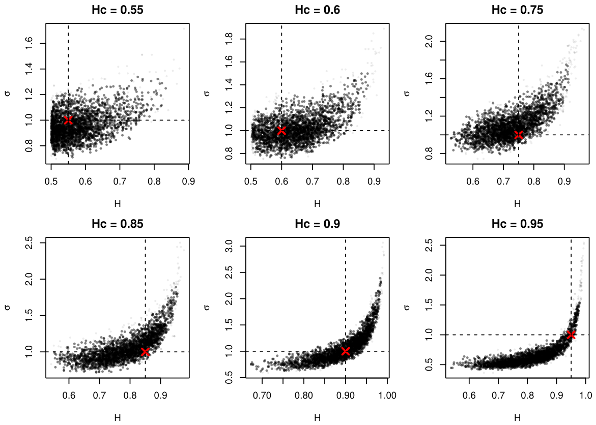
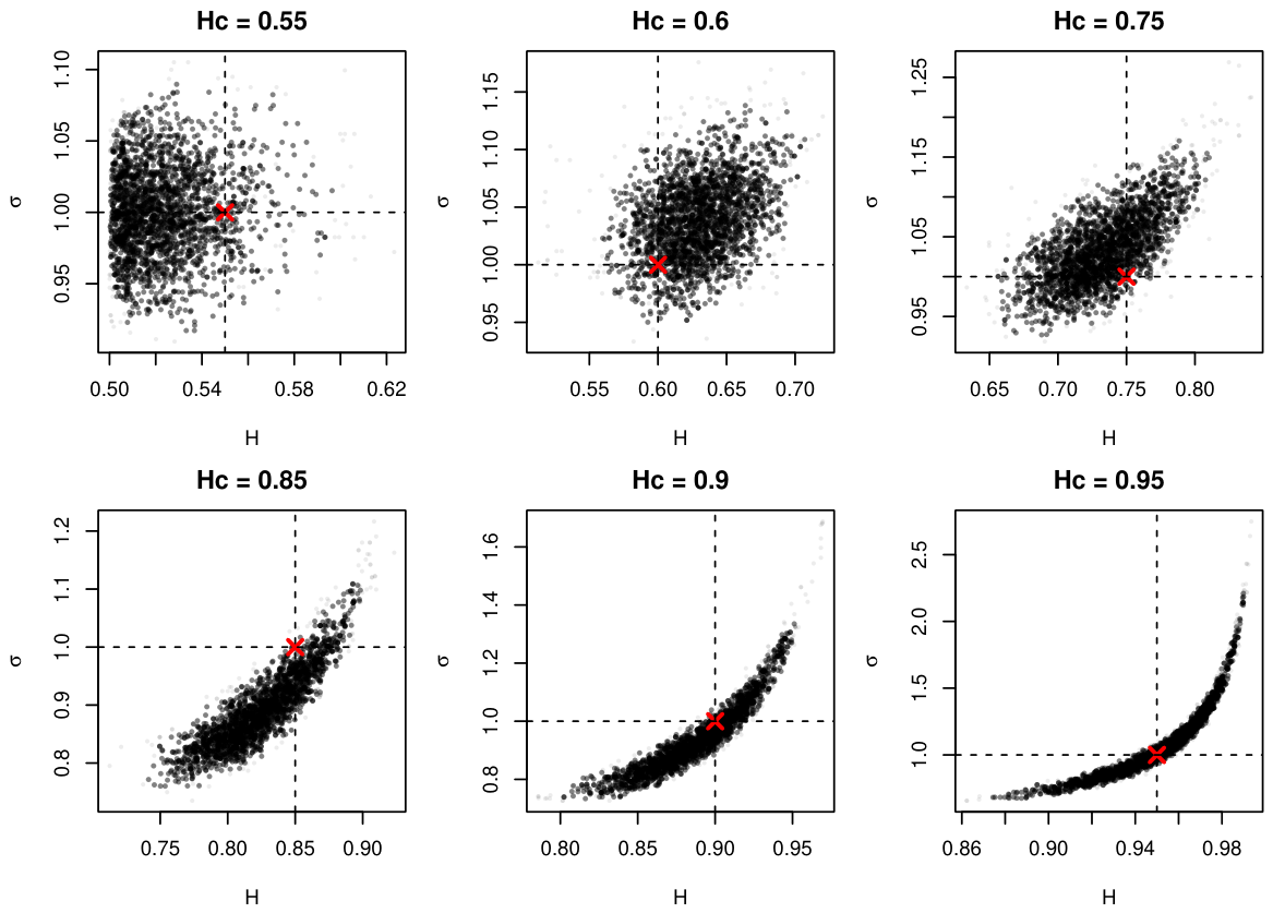
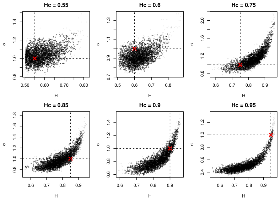
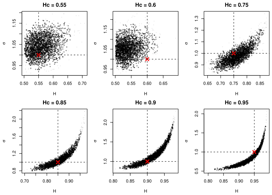
Figure 1 and Figure 2 illustrate the joint posterior draws and corresponding 95% HDR clouds for the smallest and largest sample sizes considered. These figures demonstrate the substantial posterior dependence between H and $\sigma$ and show the improvement in posterior concentration as sample size increases. Corresponding results for the intermediate sample sizes $n=100$ and $n=300$ are provided in Appendix A. 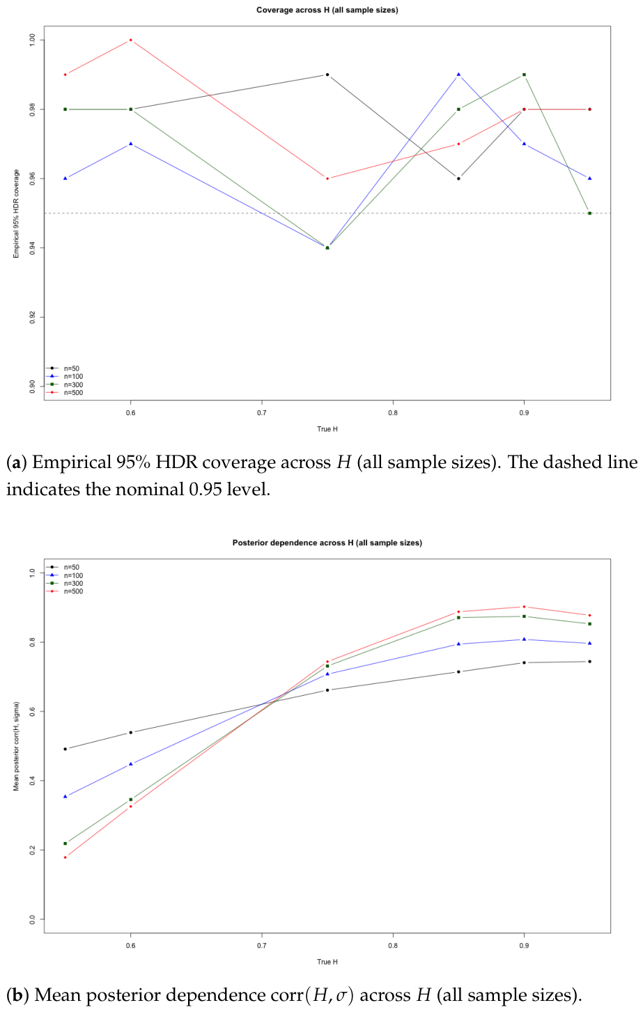Figure 3a,b summarize empirical coverage and posterior dependence across sample sizes on a common scale. Coverage remains close to the nominal 0.95 level across most settings, while $\mathrm{corr}(H,\sigma )$ generally increases with $H_c$, indicating that separate marginal intervals may fail to capture important joint posterior structure.

To quantify the Monte Carlo uncertainty associated with the empirical coverage estimates, Monte Carlo standard errors (MCSEs) were computed as

$$\mathrm{MCSE}\left(\widehat{p}\right)=\sqrt{{\displaystyle \frac{\widehat{p}(1-\widehat{p})}{B}}},$$

where $\widehat{p}$ denotes the estimated coverage probability and $B=100$ is the number of Monte Carlo replications. The MCSE values, reported in

Table 1. Simulation performance based on $B=100$ replications. The data were generated with $\mu =0$ and ${\sigma }_0=1$. Coverage is the proportion of replications in which the true pair $(H_c,{\sigma }_0)$ lies within the estimated 95% joint HDR. The Monte Carlo standard error is $\mathrm{MCSE}={\{\widehat{p}(1-\widehat{p})/B\}}^{1/2}$. The quantities ${\mathrm{Bias}}_H$ and ${\mathrm{Bias}}_{\sigma }$ denote the average posterior-median biases, and ${\overline{\rho }}_{H,\sigma }$ denotes the mean posterior correlation.

n	${\mathit{H}}_{\mathit{c}}$	Coverage	MCSE	Bias (H)	Bias ($\mathit{\sigma }$)	Mean Corr $(\mathit{H},\mathit{\sigma })$
50	0.55	0.98	0.0140	0.0617	0.0213	0.4914
50	0.60	0.98	0.0140	0.0379	0.0495	0.5392
50	0.75	0.99	0.0099	−0.0204	0.0103	0.6613
50	0.85	0.96	0.0196	−0.0541	−0.0550	0.7143
50	0.90	0.98	0.0140	−0.0542	−0.0970	0.7407
50	0.95	0.98	0.0140	−0.0641	−0.2362	0.7440
100	0.55	0.94	0.0237	0.0250	0.0226	0.3538
100	0.60	0.98	0.0140	0.0152	0.0265	0.4477
100	0.75	0.96	0.0196	0.0007	0.0274	0.7076
100	0.85	0.98	0.0140	−0.0182	−0.0043	0.7941
100	0.90	0.98	0.0140	−0.0199	−0.0314	0.8077
100	0.95	0.99	0.0099	−0.0341	−0.1552	0.7962
300	0.55	0.98	0.0140	0.0081	−0.0004	0.2188
300	0.60	0.98	0.0140	0.0057	0.0113	0.3457
300	0.75	0.94	0.0237	−0.0040	0.0072	0.7310
300	0.85	0.98	0.0140	0.0006	0.0148	0.8708
300	0.90	0.99	0.0099	−0.0106	−0.0102	0.8743
300	0.95	0.95	0.0218	−0.0215	−0.1101	0.8526
500	0.55	0.97	0.0171	0.0010	0.0036	0.1787
500	0.60	0.93	0.0255	0.0050	0.0065	0.3258
500	0.75	0.96	0.0196	0.0017	0.0092	0.7437
500	0.85	0.97	0.0171	−0.0054	−0.0052	0.8876
500	0.90	0.98	0.0140	−0.0065	−0.0024	0.9022
500	0.95	0.98	0.0140	−0.0148	−0.0809	0.8774

, ranged from approximately 0.01 to 0.03 across all simulation settings, indicating that the empirical coverage estimates are reasonably precise despite using only 100 Monte Carlo replications.

It is well known that fractional Brownian motion models may violate the semimartingale structure underlying classical arbitrage-free pricing theory (Biagini et al. 2008; Cheridito 2003; Rogers 1997). Consequently, the fractional Black–Scholes framework is used here primarily as a sensitivity-based tool for studying how posterior uncertainty in $(H,\sigma )$ propagates into option values, rather than as a complete market equilibrium model under all fractional specifications. Nevertheless, recent developments in rough volatility modeling further support the usefulness of fractional dynamics as flexible representations of financial dependence structures (Bennedsen et al. 2022; Gatheral et al. 2018).

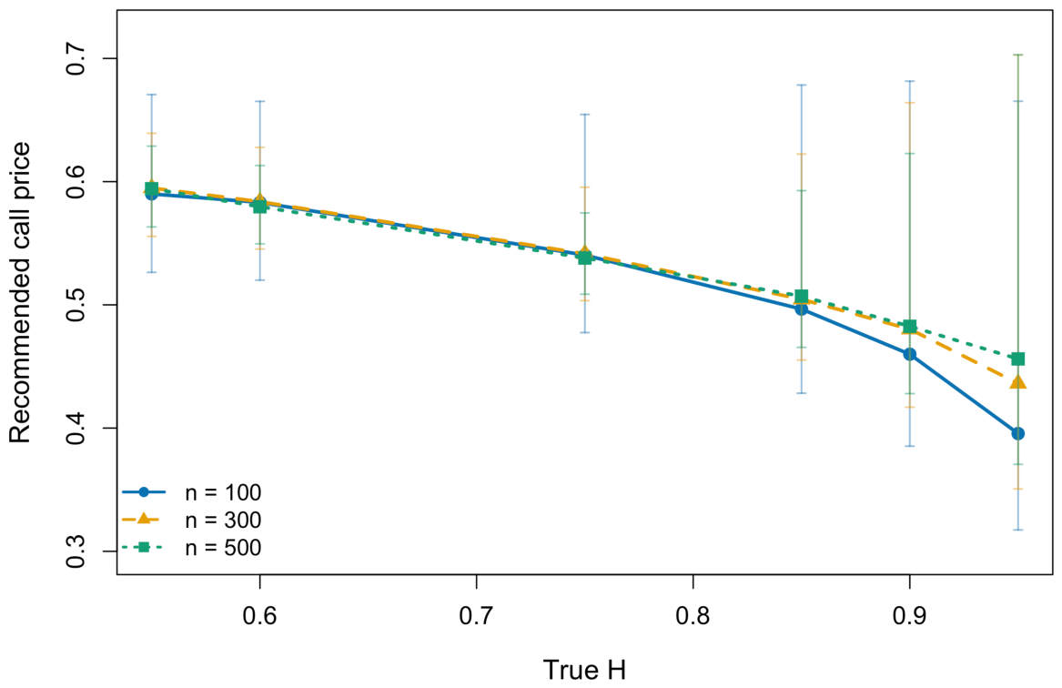
To quantify the implications for option valuation, Figure 4 reports posterior medians and 95% credible intervals for the call price obtained by mapping posterior draws $(H,\sigma )$ through the fractional Black–Scholes pricing equation. The results show a clear decline in the posterior median call price as $H_c$ increases, with the decrease becoming especially pronounced when $H_c$ approaches one. This behavior indicates that, under the chosen option-pricing parameters, stronger persistence is associated with lower posterior median call prices under the chosen option-pricing specification. More importantly, the proposed Bayesian framework quantifies the full posterior uncertainty associated with these prices, allowing uncertainty in both the Hurst parameter and volatility to be propagated directly into option valuation rather than relying solely on point estimates.

The option-pricing results exhibit the same qualitative pattern. Increasing the sample size reduces posterior uncertainty in option prices, leading to narrower credible intervals. The improvement is most pronounced when the true Hurst parameter is large because stronger long-range dependence reduces the effective information contained in the observed data, thereby increasing uncertainty in the estimated model parameters.

From a practical perspective, however, for the range of Hurst parameters typically reported in financial return series, where H is often close to 0.5, the posterior summaries obtained with $n=100$ are already reasonably stable and provide competitive pricing performance at substantially lower computational cost. Larger sample sizes become particularly beneficial when stronger persistence ($H\gtrsim 0.75$) is anticipated, where the additional information yields more noticeable reductions in posterior uncertainty and narrower credible intervals for option prices.

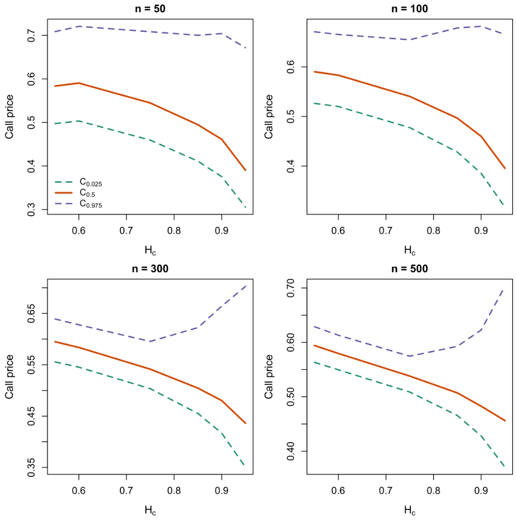
Figure 5 displays the posterior lower, median, and upper quantile curves of the option price as functions of the true Hurst parameter $H_c$ for each sample size. The lower and upper curves form a 95% credible interval. The shrinkage of the gap between $C_{0.025}$ and $C_{0.975}$ as n increases illustrates posterior concentration in the joint parameter space. The median call price decreases with $H_c$ under the chosen option parameters, while uncertainty is substantially larger for small samples and tightens as n increases. These quantile curves also facilitate decision-oriented summaries, such as one-sided credible bounds, which may be preferable when overpricing and underpricing have asymmetric consequences. Numerical values for the posterior call-price quantiles are provided in

Table 2. Posterior call-price quantiles obtained by propagating posterior draws of $(H,\sigma )$ through the fractional Black–Scholes pricing function. The interval $[C_{0.025},C_{0.975}]$ is the central 95% posterior credible interval, while $[C_{0.05},C_{0.95}]$ is the central 90% posterior interval.

n	${\mathit{H}}_{\mathit{c}}$	${\mathit{C}}_{0.025}$	${\mathit{C}}_{0.05}$	${\mathit{C}}_{0.50}$	${\mathit{C}}_{0.95}$	${\mathit{C}}_{0.975}$
50	0.55	0.4974	0.5097	0.5836	0.6840	0.7085
50	0.60	0.5033	0.5153	0.5904	0.6947	0.7206
50	0.75	0.4593	0.4710	0.5447	0.6685	0.7083
50	0.85	0.4110	0.4215	0.4948	0.6471	0.7001
50	0.90	0.3755	0.3857	0.4613	0.6427	0.7040
50	0.95	0.3054	0.3143	0.3901	0.6005	0.6716
100	0.55	0.5243	0.5356	0.5955	0.6561	0.6706
100	0.60	0.5167	0.5293	0.5863	0.6502	0.6652
100	0.75	0.4413	0.4545	0.5456	0.6590	0.6775
100	0.85	0.4092	0.4211	0.5044	0.6503	0.6696
100	0.90	0.3838	0.3956	0.4762	0.6419	0.6664
100	0.95	0.3056	0.3167	0.4141	0.5901	0.6168
300	0.55	0.5534	0.5616	0.5898	0.6318	0.6392
300	0.60	0.5456	0.5511	0.5832	0.6204	0.6278
300	0.75	0.4921	0.5007	0.5380	0.5929	0.6012
300	0.85	0.4496	0.4566	0.5053	0.5814	0.5908
300	0.90	0.4187	0.4259	0.4810	0.5802	0.5904
300	0.95	0.3382	0.3461	0.4283	0.5654	0.5866
500	0.55	0.5644	0.5680	0.5941	0.6229	0.6288
500	0.60	0.5510	0.5541	0.5812	0.6074	0.6131
500	0.75	0.4956	0.5024	0.5371	0.5886	0.5948
500	0.85	0.4427	0.4487	0.4989	0.5719	0.5800
500	0.90	0.4256	0.4302	0.4829	0.5693	0.5773
500	0.95	0.3526	0.3602	0.4379	0.5863	0.6064

.

Comparison with Classical Estimators

To further evaluate the proposed Bayesian estimator, we compared its performance with two widely used alternatives: the exact Gaussian profile maximum likelihood estimator (MLE) and the semiparametric local Whittle estimator. The comparison was conducted using the same fractional Gaussian noise datasets employed in the Bayesian simulation study so that all estimators were evaluated under identical simulation settings. Results are reported for sample sizes $n\in \{100,300\}$ and true Hurst parameters $H_c\in \{0.55,0.75,0.90\}$.

Table 3. Comparison of the proposed Bayesian estimator with the exact Gaussian profile maximum likelihood estimator (MLE) and the semiparametric local Whittle estimator. Results are based on $B=100$ Monte Carlo replications. Mean Estimate denotes the average estimated Hurst parameter, RMSE is the root mean squared error, SD is the empirical standard deviation of the estimates, and Out-of-range is the proportion of estimates outside the admissible parameter space $(0.5,1)$.

n	${\mathit{H}}_{\mathit{c}}$	Method	Mean Estimate	Bias	RMSE	SD	Out-of-Range
100	0.55	Bayesian	0.5802	0.0302	0.0495	0.0394	0.00
100	0.55	Exact MLE	0.5374	−0.0126	0.0460	0.0444	0.00
100	0.55	Local Whittle	0.5496	−0.0004	0.1305	0.1312	0.39
100	0.75	Bayesian	0.7521	0.0021	0.0653	0.0656	0.00
100	0.75	Exact MLE	0.7259	−0.0241	0.0762	0.0727	0.00
100	0.75	Local Whittle	0.7651	0.0151	0.1354	0.1352	0.03
100	0.90	Bayesian	0.8774	−0.0226	0.0516	0.0467	0.00
100	0.90	Exact MLE	0.8601	−0.0399	0.0744	0.0631	0.00
100	0.90	Local Whittle	0.9203	0.0203	0.0845	0.0824	0.00
300	0.55	Bayesian	0.5618	0.0118	0.0316	0.0294	0.00
300	0.55	Exact MLE	0.5456	−0.0044	0.0343	0.0342	0.00
300	0.55	Local Whittle	0.5561	0.0061	0.0816	0.0818	0.23
300	0.75	Bayesian	0.7583	0.0083	0.0395	0.0388	0.00
300	0.75	Exact MLE	0.7470	−0.0030	0.0392	0.0393	0.00
300	0.75	Local Whittle	0.7635	0.0135	0.0807	0.0800	0.00
300	0.90	Bayesian	0.8913	−0.0087	0.0289	0.0277	0.00
300	0.90	Exact MLE	0.8818	−0.0182	0.0372	0.0326	0.00
300	0.90	Local Whittle	0.9072	0.0072	0.0734	0.0734	0.00

summarizes the estimation performance in terms of the mean estimate, empirical bias, root mean squared error (RMSE), empirical standard deviation, and the proportion of inadmissible estimates.

Overall, the Bayesian estimator and the exact Gaussian MLE exhibited comparable estimation accuracy across the simulated settings. The Bayesian estimator achieved the smallest RMSE in four of the six simulation settings, primarily for moderate and strong persistence ($H_c=0.75$ and $0.90$), whereas the exact Gaussian MLE achieved a slightly smaller RMSE for the weakest persistence case $(n=100, H_c=0.55)$.

Although the local Whittle estimator produced relatively small average bias in several settings, it exhibited substantially larger sampling variability, leading to noticeably larger RMSE values. Moreover, the local Whittle estimator occasionally produced estimates outside the admissible parameter space $(0.5,1)$, with out-of-range rates reaching 39% for $(n=100, H_c=0.55)$ and 23% for $(n=300, H_c=0.55)$. In contrast, both the Bayesian estimator and the exact Gaussian MLE consistently produced admissible estimates across all simulation settings.

While the exact Gaussian MLE is computationally faster because it produces point estimates through direct likelihood optimization, the proposed Bayesian methodology provides full posterior inference for the Hurst parameter and volatility simultaneously. This enables posterior uncertainty to be propagated directly into option pricing, yielding posterior credible intervals for derivative prices in addition to point estimates. Consequently, the proposed framework combines competitive estimation accuracy with full posterior uncertainty quantification for fractional option pricing.

As an additional robustness assessment, we performed a larger Monte Carlo experiment with sample size $n=500$ and $B=200$ replications. The conclusions remained unchanged. In an additional Monte Carlo study with $n=500$ and $H_c\in \{0.55,0.75,0.90\}$, the proposed Bayesian estimator exhibited negligible bias (absolute bias below 0.006) and RMSE values below 0.032. It also achieved slightly smaller bias and RMSE than the exact Gaussian MLE for the additional simulation settings considered, while providing full posterior uncertainty quantification. In contrast, the local Whittle estimator continued to display substantially larger sampling variability and produced inadmissible estimates outside the parameter space $(0.5,1)$ in approximately 21.5% of the replications when $H=0.55$. These additional experiments further support the robustness and numerical stability of the proposed Bayesian framework.

4. Empirical Application

This section illustrates the practical performance of the proposed Bayesian framework using real financial data from energy markets. We consider daily log returns of WTI crude oil and natural gas futures, which represent two economically important commodity markets with distinct volatility characteristics and substantial relevance for derivative-pricing applications.

WTI crude oil is examined over two market regimes. The period 2020–2022 represents a high-volatility environment, whereas 2023–2025 reflects comparatively more stable market conditions. Natural gas is included as an additional example of a persistently volatile energy market. This design allows the proposed methodology to be evaluated across contrasting volatility environments while holding the general modeling framework fixed.

For each dataset, the Hurst parameter and volatility are estimated jointly using the Bayesian methodology developed in Section 2. The resulting posterior draws are then propagated through the fractional Black–Scholes pricing function to obtain a posterior distribution of option prices. In addition to posterior medians and credible intervals, we report posterior expectations and variances of the induced option-price distributions to characterize both expected values and pricing uncertainty.

The empirical contribution is not merely to confirm the expected observation that higher volatility is associated with greater pricing uncertainty. Rather, the proposed framework provides a probabilistic sensitivity analysis that quantifies how uncertainty in both model parameters, together with their posterior dependence, propagates into option valuation. This joint treatment helps distinguish volatility-driven pricing effects from those associated with long-range dependence and provides information that is not available from separate point estimates alone.

The empirical section also examines the robustness and reliability of the posterior analysis through prior sensitivity checks and standard MCMC convergence diagnostics. Additional analyses based on alternative sampling frequencies are used to assess whether the estimated persistence depends on the temporal resolution of the return series.

4.1. WTI Crude Oil: Regime Comparison

We begin with WTI crude oil, which exhibits distinct market regimes. The period 2020–2022 corresponds to elevated market volatility, whereas 2023–2025 reflects comparatively more stable conditions. These two periods provide a natural setting for investigating how different volatility regimes influence the joint posterior distribution of the Hurst parameter and volatility and the resulting posterior distribution of option prices.

Table 4. Summary statistics for the WTI crude oil return series used in the empirical analysis.

Asset	Ticker	Period	n	Mean Return	Annualized Volatility
WTI Crude Oil	CL=F	2020–2022	522	0.00185	0.698
WTI Crude Oil	CL=F	2023–2025	752	$-0.00038$	0.315

shows that the earlier period exhibits substantially higher annualized volatility, whereas the average daily returns remain close to zero in both regimes. This suggests that the principal distinction between the two periods is the level of market variability rather than systematic differences in expected returns.

For pricing, we consider a European call option with $S_0=100$, $K=98$, $T=90/365$, and $r=0.05$. These contract specifications are held fixed throughout the empirical analysis so that differences in the posterior option-price distributions are attributable solely to changes in the estimated model parameters rather than changes in the option contract itself. The selected contract specifications correspond to a representative near-the-money option with a short time to maturity and serve as a common benchmark for comparing pricing uncertainty across the different empirical datasets and market regimes.

Table 5. Posterior summaries and option pricing results for WTI crude oil across two market periods. Mean and SD denote the posterior expectation and posterior standard deviation of the option price obtained from the joint posterior distribution of the Hurst parameter and volatility under the fractional Black–Scholes model. L95 and U95 denote the lower and upper limits of the 95% posterior credible interval, respectively. Width denotes the length of the 95% posterior credible interval.

Period	H (95% CI)	$\mathit{\sigma }$	BSM	Mean	SD	Median	L95	U95	Width
2020–2022	0.529 (0.501, 0.585)	0.698	15.15	15.01	0.43	14.99	14.20	15.88	1.69
2023–2025	0.514 (0.500, 0.552)	0.315	7.86	7.83	0.16	7.83	7.53	8.13	0.61

reports posterior summaries for the Hurst parameter, volatility, and the induced option-price distribution. Across both periods, the posterior estimates of the Hurst parameter remain close to 0.5, indicating only weak evidence of long-range dependence in daily returns, whereas the posterior volatility differs substantially between the two market regimes.

The posterior mean and posterior median option prices are nearly identical, suggesting little evidence of posterior skewness. In contrast, the posterior standard deviation increases from 0.16 during the lower-volatility period to 0.43 during the high-volatility period, quantifying the substantial increase in option-pricing uncertainty associated with elevated market volatility.

Although greater pricing uncertainty during the high-volatility period is expected, the principal contribution of the proposed Bayesian framework is not simply to confirm this relationship. Rather, it quantifies how uncertainty in both model parameters propagates through the fractional Black–Scholes model into the posterior distribution of option prices. Consequently, the posterior expectation, posterior standard deviation, and credible intervals provide a probabilistic sensitivity analysis of option valuation rather than a single deterministic price.

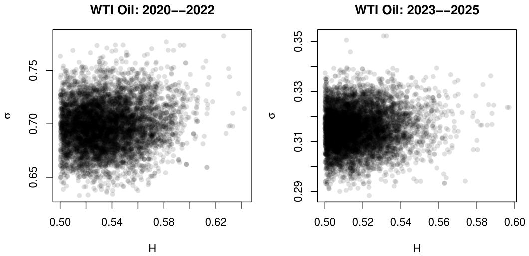
Figure 6 further illustrates that the posterior distribution of the Hurst parameter remains relatively stable across periods, whereas volatility exhibits substantial variation between market regimes. The posterior clouds also reveal noticeable dependence between H and $\sigma$, emphasizing the importance of joint uncertainty quantification in the Bayesian framework. The positive posterior dependence observed between the Hurst parameter and volatility further demonstrates that these parameters should not be assessed independently when quantifying option-pricing uncertainty. This dependence further motivates the use of joint highest-density regions rather than separate marginal credible intervals. The joint posterior distribution also illustrates that uncertainty in option prices cannot be attributed solely to either parameter in isolation but instead arises from their joint posterior behavior.

The fractional Black–Scholes formula is used here as a sensitivity-based pricing framework to study how posterior uncertainty in $(H,\sigma )$ propagates into option values, rather than as a claim of complete market arbitrage-free dynamics under all fractional specifications. Although the fractional Black–Scholes framework does not explicitly incorporate commodity-specific features such as mean reversion or stochastic convenience yields, the objective here is not to develop a complete structural model for commodity markets. Instead, the framework is used to investigate how uncertainty in the two model parameters propagates into option prices under the assumed fractional pricing model. Consequently, the empirical results should be interpreted as conditional on this modeling framework. Future research could extend the proposed Bayesian framework by embedding fractional dynamics within commodity pricing models that explicitly account for mean reversion and stochastic convenience yields, thereby allowing uncertainty quantification under more realistic commodity-market dynamics.

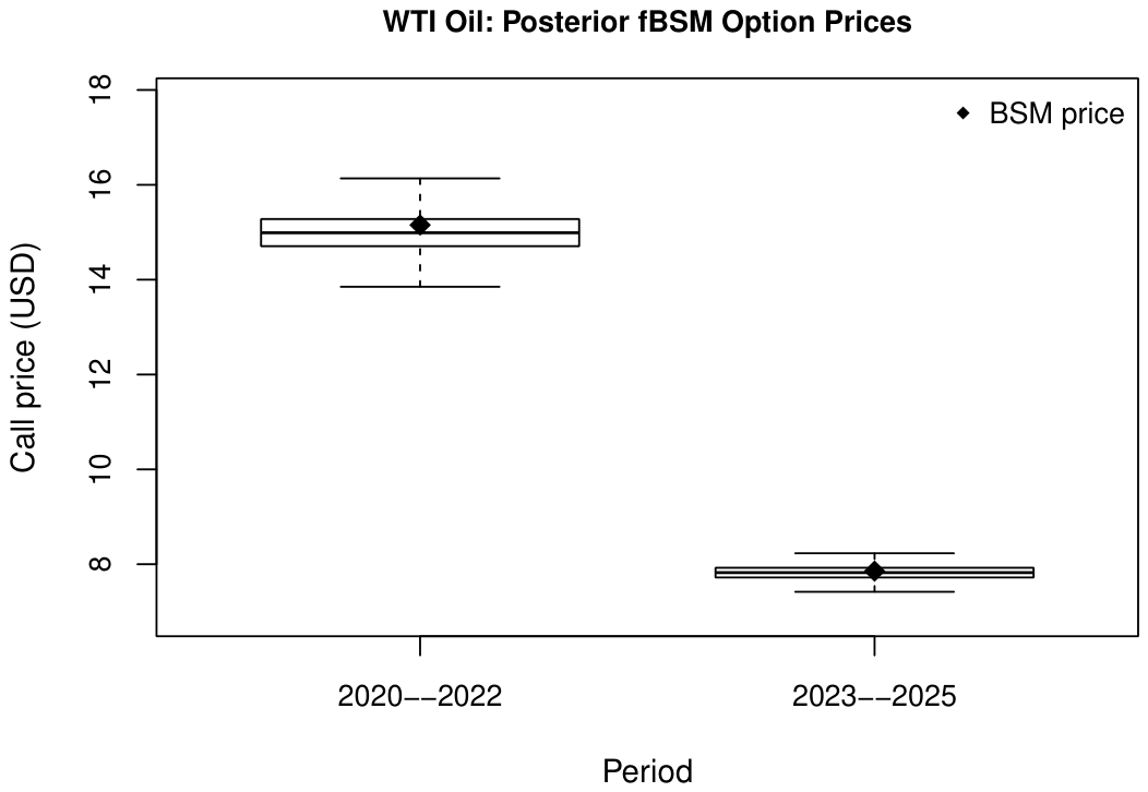
Figure 7 shows that the high-volatility period produces a substantially wider posterior distribution of option prices, reflecting increased pricing uncertainty. In contrast, the more stable 2023–2025 regime yields a considerably tighter distribution. Although the posterior median prices remain reasonably close to the corresponding classical Black–Scholes prices, the range of plausible option values differs substantially across market regimes.

Overall, the analysis indicates that posterior uncertainty in option prices is driven primarily by volatility in the daily WTI crude oil data, whereas the estimated Hurst parameter remains close to the classical Brownian motion value. More importantly, the proposed Bayesian methodology provides a direct probabilistic characterization of how uncertainty in both model parameters propagates into the posterior distribution of option prices, yielding substantially richer information for uncertainty assessment and risk analysis than is available from point estimates alone.

4.2. Natural Gas: High-Volatility Market

We next consider natural gas as an example of a persistently high-volatility commodity market. Unlike the regime comparison for WTI crude oil, the natural gas data represent a single market environment characterized by sustained volatility. This provides an opportunity to evaluate the proposed Bayesian framework when parameter uncertainty is consistently elevated and to examine whether option-pricing uncertainty is driven primarily by volatility or by long-range dependence.

Table 6. Summary statistics for the natural gas return series used in the empirical analysis.

Asset	Ticker	Period	n	Mean Return	Annualized Volatility
Natural Gas Futures	NG=F	2022–2024	250	$-0.00255$	0.787

shows that the return series is characterized by high annualized volatility, while the average daily return remains close to zero. These characteristics are consistent with the well-known variability of natural gas markets and motivate an investigation of how parameter uncertainty affects option pricing.

For pricing, we consider the same European call option with $S_0=100$, $K=98$, $T=90/365$, and $r=0.05$. Holding these contract specifications fixed allows differences in the posterior option-price distributions to be attributed solely to changes in the estimated model parameters. This provides a common benchmark for comparing pricing uncertainty across the empirical applications.

Table 7. Posterior summaries and option pricing results for natural gas. Mean and SD denote the posterior expectation and posterior standard deviation of the option price obtained from the joint posterior distribution of the Hurst parameter and volatility under the fractional Black–Scholes model. L95 and U95 denote the lower and upper limits of the 95% posterior credible interval, respectively. Width denotes the length of the 95% posterior credible interval.

Period	H (95% CI)	$\mathit{\sigma }$	BSM	Mean	SD	Median	L95	U95	Width
2022–2023	0.515 (0.500, 0.568)	0.787	16.91	16.90	0.69	16.87	15.58	18.30	2.72

reports posterior summaries for the Hurst parameter, volatility, and the induced option-price distribution. The posterior estimate of the Hurst parameter remains close to 0.5, indicating only weak evidence of long-range dependence in the daily returns. In contrast, the posterior volatility is substantially larger than that observed for the lower-volatility WTI regime.

The posterior mean and posterior median option prices are nearly identical, suggesting little evidence of substantial posterior skewness. The posterior standard deviation of the option price is 0.69, which is considerably larger than that observed for either WTI regime. This indicates substantially greater uncertainty in option valuation under the highly volatile natural gas market.

These results suggest that volatility is the dominant contributor to option-pricing uncertainty for the natural gas data. Rather than indicating a strong effect of long-range dependence on option valuation, the Bayesian analysis shows that the Hurst parameter contributes relatively little additional uncertainty once its posterior distribution is jointly considered with the volatility parameter. Consequently, the posterior expectation, posterior standard deviation, and credible intervals provide a probabilistic sensitivity analysis of the relative contributions of these two sources of uncertainty.

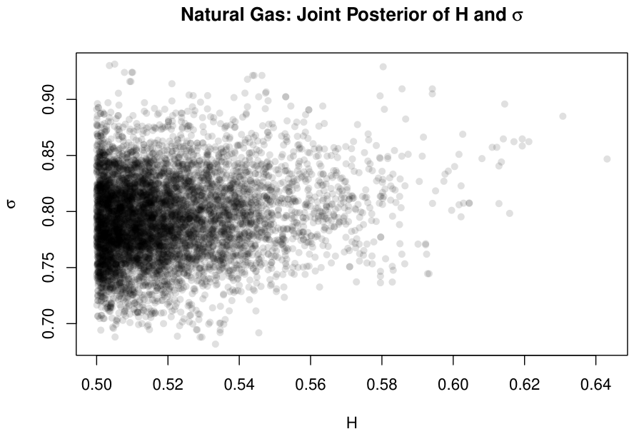
The joint posterior distribution in Figure 8 illustrates that uncertainty is dominated by the volatility parameter, whereas the posterior distribution of the Hurst parameter remains tightly concentrated around 0.5. The positive posterior dependence between the two parameters nevertheless demonstrates that they should be estimated jointly rather than independently when quantifying option-pricing uncertainty.

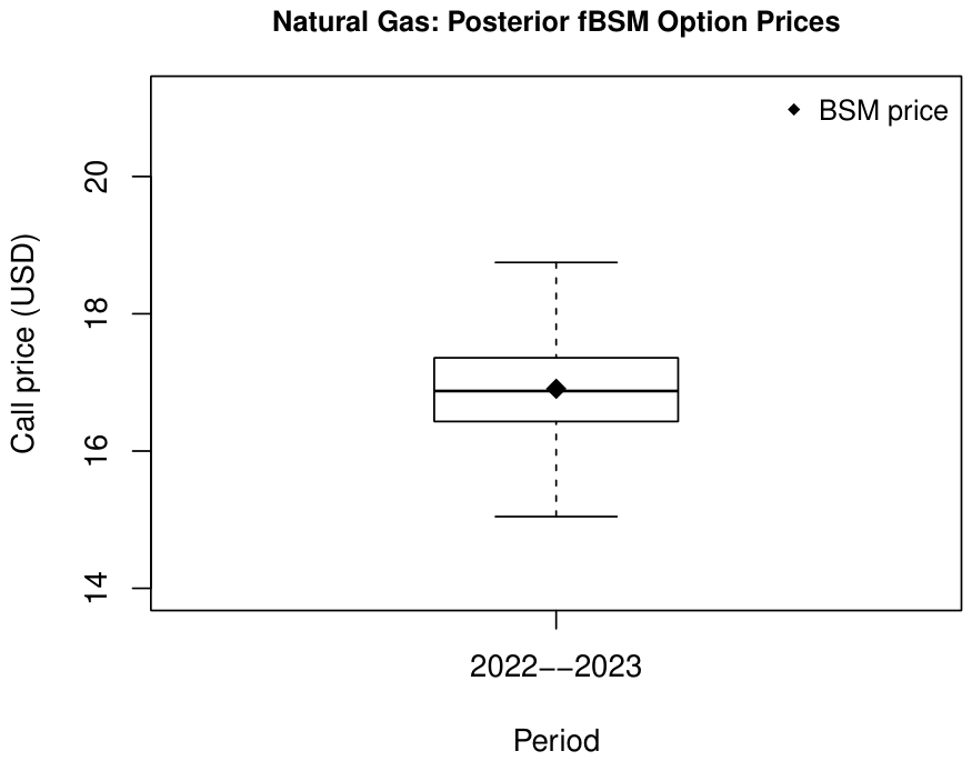
Figure 9 shows that the posterior distribution of option prices is substantially wider than would be suggested by the single Black–Scholes price. Although the Black–Scholes price lies within the posterior credible interval, it represents only a point estimate and therefore does not capture the uncertainty arising from the joint posterior distribution of the Hurst parameter and volatility.

Overall, the natural gas application demonstrates that posterior uncertainty in option prices is driven primarily by volatility, whereas the estimated Hurst parameter remains close to the classical Brownian-motion value. More importantly, the proposed Bayesian framework provides a direct probabilistic characterization of how uncertainty in both model parameters propagates into the posterior distribution of option prices, thereby distinguishing the relative contributions of volatility and long-range dependence to pricing uncertainty. This illustrates the value of the proposed methodology as a probabilistic sensitivity-analysis framework rather than simply a point-estimation procedure.

4.3. Effect of Daily and Weekly Sampling Frequencies

To investigate the effect of temporal aggregation on posterior inference, we compare Bayesian estimation based on daily and weekly returns for both WTI crude oil and natural gas. Financial time series may exhibit different dependence structures across sampling frequencies, since weekly aggregation can smooth short-term fluctuations while emphasizing longer-term persistence. Because the proposed Bayesian framework jointly estimates the Hurst parameter and volatility, changes in sampling frequency may affect not only posterior parameter estimates but also the propagation of uncertainty into option prices.

Table 8. Comparison of posterior summaries obtained from daily and weekly WTI crude oil returns. Mean and SD denote the posterior expectation and posterior standard deviation of the option price under the fractional Black–Scholes model, and Width denotes the length of the 95% posterior credible interval.

Frequency	H (95% CI)	$\mathit{\sigma }$	Corr	BSM	Mean	SD	Median	95% CI	Width
Daily	0.530 (0.501, 0.584)	0.698	0.119	15.17	15.02	0.43	15.00	(14.20, 15.90)	1.71
Weekly	0.712 (0.558, 0.850)	0.637	0.665	13.39	12.76	0.81	12.69	(11.37, 14.52)	3.15

demonstrates that the inferred Hurst parameter is sensitive to the sampling frequency. Using daily returns, the posterior median is 0.530, indicating weak evidence of long-range dependence. In contrast, weekly aggregation increases the posterior median to 0.712, with the credible interval extending well above 0.5, suggesting substantially stronger persistence.

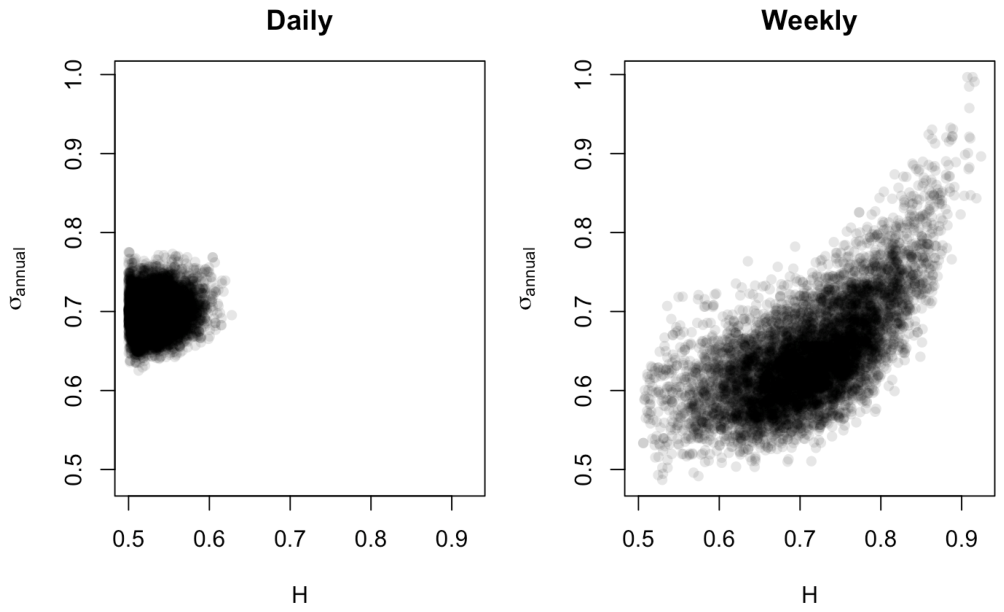
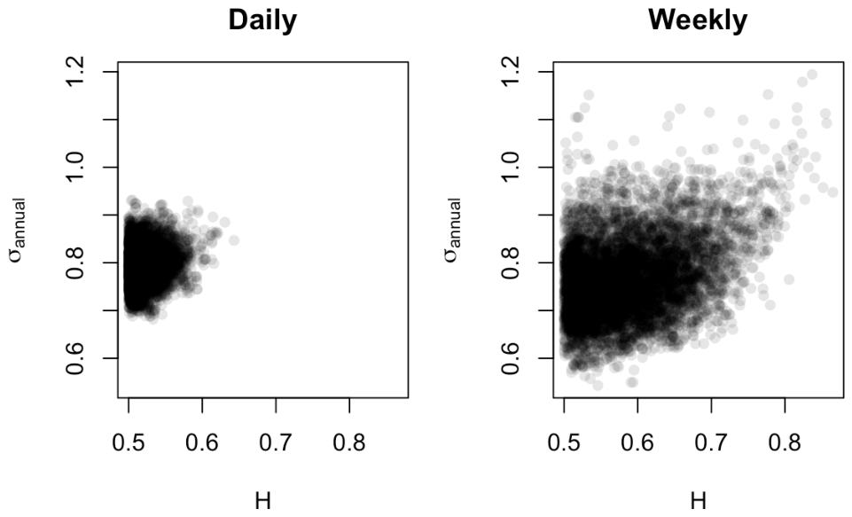
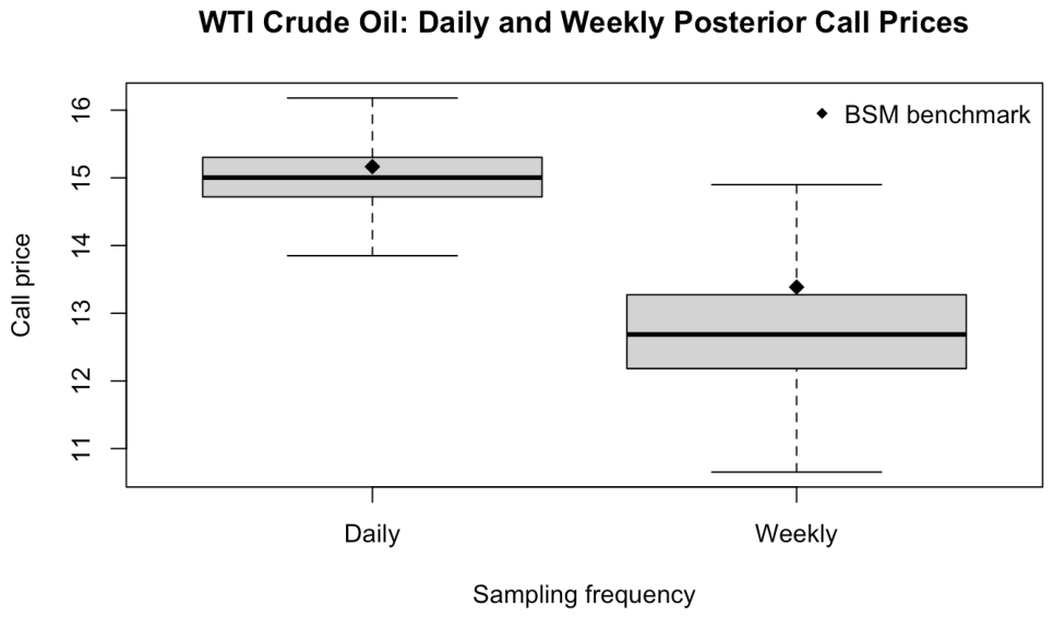
Although the posterior annualized volatility decreases slightly after weekly aggregation, the dependence between the Hurst parameter and volatility increases markedly, with the posterior correlation rising from 0.12 to 0.66 (Figure 10). This stronger posterior dependence leads to much greater uncertainty propagation into option prices. The posterior standard deviation nearly doubles from 0.43 to 0.81, while the width of the 95% posterior credible interval increases from 1.71 to 3.15. Consequently, weekly data produce substantially greater uncertainty in option valuation despite exhibiting slightly lower estimated volatility (Figure 11).

The same qualitative behavior is observed for natural gas (

Table 9. Comparison of posterior summaries obtained from daily and weekly natural gas returns. Mean and SD denote the posterior expectation and posterior standard deviation of the option price under the fractional Black–Scholes model, and Width denotes the length of the 95% posterior credible interval.

Frequency	H (95% CI)	$\mathit{\sigma }$	Corr	BSM	Mean	SD	Median	95% CI	Width
Daily	0.515 (0.500, 0.568)	0.793	0.146	16.91	16.90	0.69	16.87	(15.58, 18.30)	2.72
Weekly	0.578 (0.503, 0.740)	0.763	0.332	16.01	15.90	1.42	15.81	(13.42, 18.97)	5.55

). Weekly aggregation increases the posterior median of the Hurst parameter from 0.515 to 0.578 while producing a wider credible interval, indicating greater uncertainty in the persistence parameter. The posterior dependence between the Hurst parameter and volatility also strengthens, with the posterior correlation increasing from 0.15 to 0.33.

Overall, the results demonstrate that posterior inference is sensitive to the sampling frequency used to construct the return series. Weekly aggregation consistently produces larger posterior estimates of the Hurst parameter, stronger posterior dependence between the Hurst parameter and volatility (Figure 12), and substantially wider posterior distributions of option prices for both WTI crude oil and natural gas.

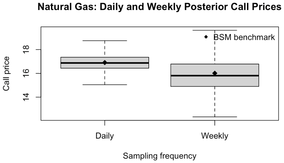
More importantly, the uncertainty associated with option pricing grows substantially under weekly sampling. The posterior standard deviation more than doubles, increasing from 0.69 to 1.42, while the width of the 95% posterior credible interval expands from 2.72 to 5.55. The wider posterior distribution is also evident in the boxplots (Figure 13), demonstrating that temporal aggregation materially affects the uncertainty propagated through the fractional Black–Scholes pricing model.

These findings indicate that the temporal resolution of the observed returns constitutes an additional source of modeling uncertainty. Consequently, the proposed Bayesian framework not only estimates model parameters but also quantifies how the choice of sampling frequency propagates through the joint posterior distribution into option-pricing uncertainty.

4.4. Prior Sensitivity Analysis

To evaluate the robustness of the proposed Bayesian framework with respect to prior specification, we performed a prior sensitivity analysis using the weekly natural gas dataset. This dataset was selected because it represents the most challenging empirical setting considered in this study, exhibiting relatively high volatility together with substantial posterior uncertainty. Demonstrating robustness in this setting provides strong evidence for the stability of the proposed Bayesian framework.

We considered four commonly used prior distributions for the volatility parameter: a Lognormal prior, a Half-Normal prior, a Half-Cauchy prior, and an Inverse-Gamma prior. The prior for the Hurst parameter remained Uniform$(0.5,1)$, while the weakly informative Normal prior for the mean parameter was unchanged.

Table 10. Prior sensitivity analysis for the weekly natural gas data under four alternative prior distributions for the volatility parameter.

Prior	H (95% CI)	$\mathit{\sigma }$	$\mathit{\sigma }$ (95% CI)
Lognormal	0.579 (0.504, 0.754)	0.768	(0.629, 0.994)
Half-Normal	0.578 (0.503, 0.735)	0.765	(0.630, 0.949)
Half-Cauchy	0.581 (0.505, 0.736)	0.765	(0.635, 0.952)
Inverse-Gamma	0.582 (0.505, 0.750)	0.755	(0.626, 0.957)

demonstrates that the posterior inference is remarkably stable across all four prior specifications. The posterior median of the Hurst parameter varies only between 0.578 and 0.582, while the corresponding 95% credible intervals largely overlap. Similarly, the posterior median of the annualized volatility remains within a narrow range of approximately 0.755–0.768 across all priors.

These results indicate that the information contained in the observed data dominates the prior assumptions, leading to highly consistent posterior inference despite substantial changes in the prior distribution for the volatility parameter. Consequently, the empirical findings are not driven by a particular prior choice but instead reflect the information provided by the weekly natural gas returns.

Overall, the limited sensitivity of the posterior estimates to the prior specification indicates that the proposed Bayesian framework is primarily data-driven for this application, thereby increasing confidence in the resulting uncertainty quantification and option-pricing inference.

4.5. MCMC Convergence Diagnostics

To assess the reliability of the posterior inference, we evaluated the convergence of the Markov chain Monte Carlo (MCMC) algorithm using the weekly natural gas dataset. This dataset was selected because it represents the most challenging empirical setting considered in this study, combining high market volatility with relatively large posterior uncertainty.

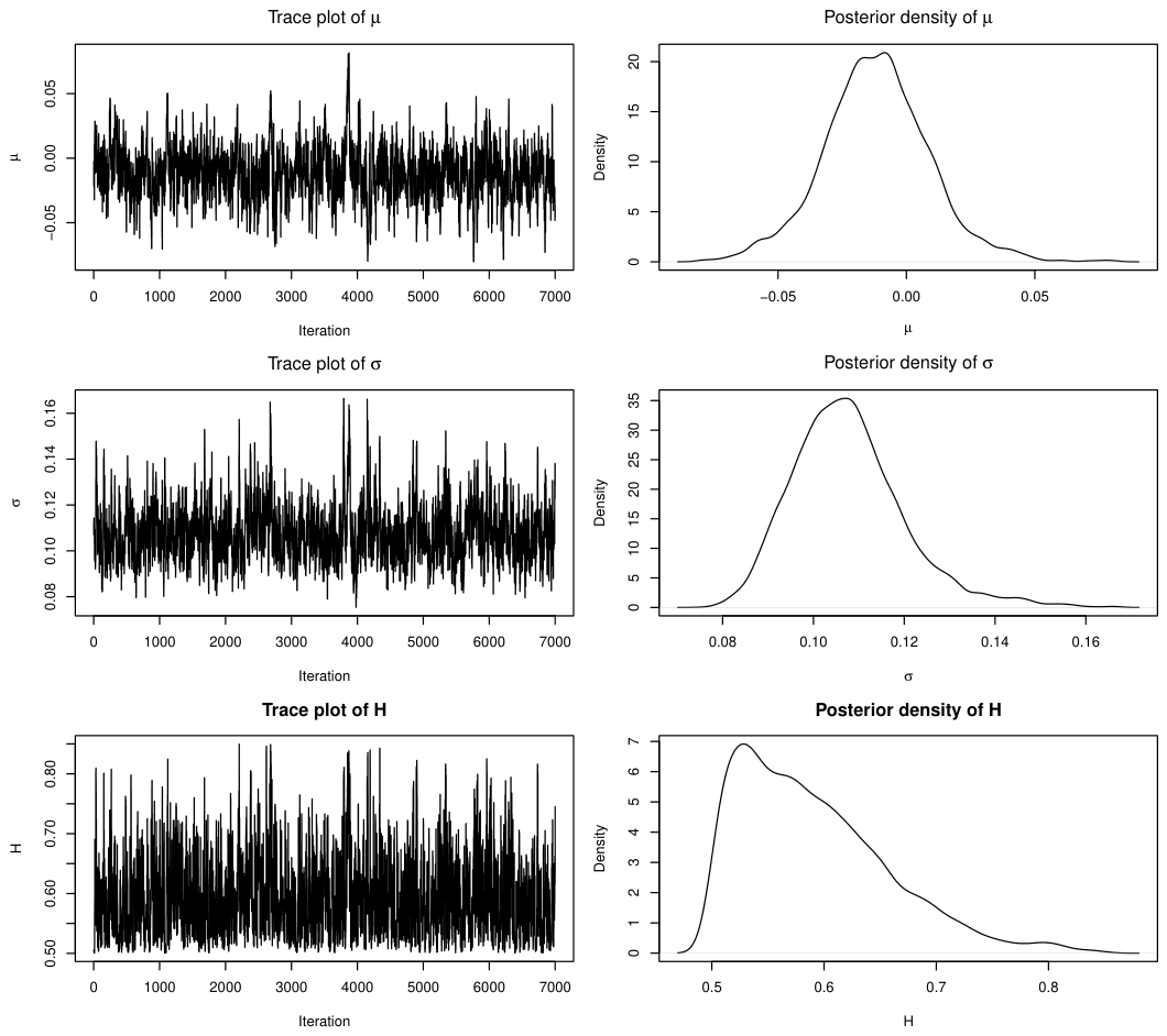
Figure 14 presents the trace plots and posterior density estimates for the mean parameter $\mu$, the volatility parameter $\sigma$, and the Hurst parameter H. The trace plots exhibit stable mixing without visible trends or abrupt shifts, while the posterior density estimates are smooth and unimodal, indicating that the Markov chains adequately explored the posterior distribution.

Table 11. MCMC convergence diagnostics for the weekly natural gas analysis. ESS denotes the effective sample size, while the Geweke diagnostic compares the early and late portions of the Markov chain.

Parameter	ESS	Geweke Z
$\mu$	424.14	1.36
$\sigma$	464.13	$-0.90$
H	669.80	$-1.68$

summarizes two commonly used convergence diagnostics. The effective sample sizes exceed 400 for all model parameters, indicating that the posterior summaries are based on a substantial number of effectively independent draws despite the autocorrelation naturally present in MCMC samples. In addition, the Geweke diagnostic yields standardized statistics between $-2$ and 2 for all parameters, providing no evidence of lack of convergence.

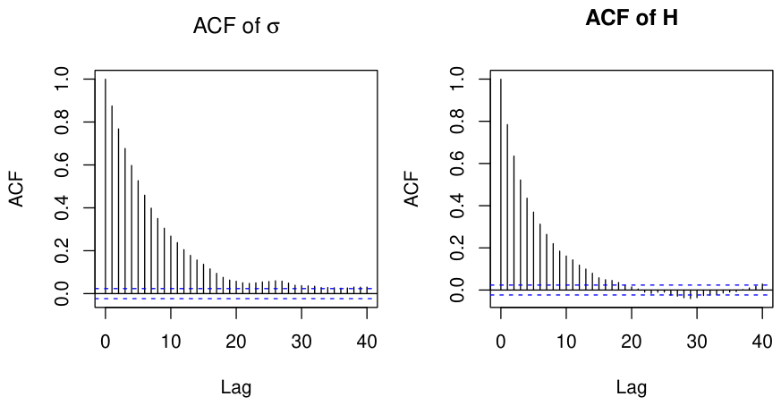
Figure 15 presents the autocorrelation functions for the posterior draws of the volatility parameter $\sigma$ and the Hurst parameter H. Although positive autocorrelation is present at short lags, it decays steadily as the lag increases, which is typical of well-behaved MCMC algorithms and is consistent with the observed effective sample sizes.

Overall, the trace plots, posterior density estimates, effective sample sizes, Geweke diagnostics, and autocorrelation analyses provide consistent evidence that the proposed MCMC algorithm achieved satisfactory convergence and mixing. Consequently, the posterior summaries reported throughout the empirical analysis can be regarded as reliable approximations to the target posterior distribution.

5. Discussion and Conclusions

This paper develops a Bayesian framework for the joint estimation of the Hurst parameter and volatility under the fractional Black–Scholes model and investigates how uncertainty in these parameters propagates into option pricing. The proposed methodology combines Bayesian inference, joint posterior uncertainty quantification, and fractional option pricing within a unified framework. Empirical analyses of WTI crude oil and natural gas futures yield several important findings.

First, the empirical analyses demonstrate that the estimated Hurst parameter depends on the temporal resolution of the observed returns. For the daily datasets, the posterior estimates generally remain close to $H=0.5$, suggesting weak evidence of long-range dependence despite periods of elevated market volatility. In contrast, weekly aggregation produces larger posterior estimates of the Hurst parameter in both applications, indicating stronger inferred persistence at the weekly frequency. The corresponding credible intervals are also wider, reflecting greater uncertainty, in part due to the smaller number of weekly observations. These findings highlight that inferences about long-range dependence are sensitive to the sampling frequency and should be interpreted alongside their associated posterior uncertainty.

For the daily datasets, the posterior distributions of the Hurst parameter are concentrated near the lower boundary of the assumed parameter space, suggesting limited evidence of persistence beyond the classical Brownian motion benchmark. Nevertheless, the posterior uncertainty surrounding H remains relevant because it is propagated jointly with uncertainty in volatility into the distribution of option prices. Since option valuation is a nonlinear function of the model parameters, even moderate posterior uncertainty may generate meaningful variation in derivative prices. From a risk-management perspective, posterior distributions therefore provide richer information than single-point estimates.

Second, volatility appears to be the principal empirical contributor to option-pricing uncertainty in the datasets considered. For WTI crude oil, the comparison of two market regimes shows that changes in volatility explain most of the observed differences in pricing uncertainty while the Hurst parameter remains relatively stable. Similarly, the natural gas application exhibits persistently high volatility, along with substantially wider posterior option price distributions. Although the Hurst parameter contributes to pricing uncertainty through its joint posterior distribution with volatility, the empirical evidence suggests that volatility is the primary determinant of uncertainty in the datasets considered.

Third, the sampling-frequency analysis demonstrates that temporal aggregation itself represents an important source of modeling uncertainty. Weekly returns produce stronger posterior dependence between the Hurst parameter and volatility, together with substantially wider posterior distributions of option prices than daily returns. These results indicate that the temporal resolution of the observed data may have a material effect on both parameter inference and derivative valuation.

From a methodological perspective, the principal contribution of the proposed framework is not the development of a new estimator for the Hurst parameter, but the integration of Bayesian parameter inference, joint uncertainty quantification, and fractional option pricing within a unified framework. Joint highest-density regions capture posterior dependence between the Hurst parameter and volatility, while propagating the retained posterior draws through the fractional Black–Scholes pricing model yields posterior expectations, posterior variances, and credible intervals for option prices. Consequently, the proposed methodology may be viewed as a probabilistic sensitivity analysis framework that quantifies how uncertainty in model parameters influences derivative valuation.

The robustness analyses further support the proposed methodology. The prior sensitivity analysis demonstrates that the posterior estimates are stable across several reasonable prior specifications for the volatility parameter, indicating that the empirical conclusions are driven primarily by the observed data rather than by prior assumptions. Furthermore, the MCMC convergence diagnostics, including trace plots, effective sample sizes, Geweke statistics, and autocorrelation analyses, provide consistent evidence of satisfactory convergence and mixing, supporting the reliability of the reported posterior summaries.

Overall, the empirical findings indicate that volatility uncertainty plays a larger role than long-range dependence uncertainty in determining option-pricing uncertainty for the assets and periods considered. At the same time, the Bayesian framework demonstrates that jointly accounting for parameter uncertainty provides substantially richer information than classical point-estimation approaches and offers a principled basis for risk assessment under fractional financial models.

The reported option prices and posterior credible intervals should be interpreted as conditional on the assumed fractional Black–Scholes model rather than as arbitrage-free market prices. Accordingly, the proposed methodology should be viewed as a tool for quantifying parameter uncertainty within the assumed fractional framework rather than as a complete arbitrage-free pricing model.

This study has several limitations. The return series are modeled using a Gaussian fractional Gaussian noise likelihood with constant volatility within each sample period. Consequently, the framework does not explicitly account for stochastic volatility, jumps, heavy tails, structural breaks, or other nonlinear features frequently observed in financial markets. In addition, parameter estimation is performed under a Gaussian fractional Gaussian noise likelihood for discrete-time log returns, whereas option pricing is based on the fractional Black–Scholes model. The reported posterior option-price distributions should therefore be interpreted as model-based quantities conditional on the assumed fractional asset-price dynamics. Furthermore, although both daily and weekly sampling frequencies were investigated, the empirical analysis does not consider intraday data, where market microstructure effects and higher-frequency dependence patterns may become important. Finally, while the empirical applications focus on commodity futures, the fractional Black–Scholes framework does not explicitly incorporate commodity-specific features such as stochastic convenience yields or mean-reverting spot-price dynamics.

Future research may extend the proposed framework by incorporating stochastic volatility, heavy-tailed likelihoods, alternative fractional processes, and more realistic commodity pricing models that explicitly account for mean reversion and stochastic convenience yields. Additional directions include applications to intraday financial data, multivariate fractional models, Bayesian model comparison, and the integration of fractional dynamics with jumps, leverage effects, and regime-switching mechanisms. Overall, the proposed Bayesian framework demonstrates that uncertainty quantification provides valuable insight into the stability, sensitivity, and reliability of option pricing under fractional financial models.